The effect of a velocity barrier on the ballistic transport of Dirac fermions

Abstract

We propose a novel way to manipulate the transport properties of massless Dirac fermions by using velocity barriers, defining the region in which the Fermi velocity, $v_{F}$, has a value that differs from the one in the surrounding background. The idea is based on the fact that when waves travel accross different media, there are boundary conditions that must be satisfied, giving rise to Snell’s-like laws. We find that the transmission through a velocity barrier is highly anisotropic, and that perfect transmission always occurs at normal incidence. When $v_{F}$ in the barrier is larger that the velocity outside the barrier, we find that a critical transmission angle exists, a Brewster-like angle for massless Dirac electrons.

When reading this paper, one is using the fact that the speed of light in vacuum is different from the speed of light in various parts of your eyes Landau et al. (1984). That difference allows our eyes and other optical devices to focus light in a very simple but efficient way. In general, when a physical object crosses a boundary, it must follow certain rules, regardless of its particle or wave-like behavior. Those rules are typically various incarnations of the well-known Snell’s law for optics.

In optics, the Snell’s law is the natural outcome of Fermat’s principle: light follows the path of least time Landau et al. (1984); Arnol’d (1989). Similar laws are found in all known oscillatory phenomena Fetter and Walecka (1980). This relation can also be found in classical mechanics in the standard problem of scattering by a constant potential barrier Landau and Lifshitz (1989). In this case, this law appears as the consequence of conservation of linear momentum in the direction parallel to the barrier and overall energy conservation. It also appears in quantum systems, and the prediction of relations analogous to Snell’s law would be of utmost importance because, as happens in optics, it will allow us to control the focusing of electrons, opening paths for new nanodevices Cheianov et al. (2007).

With the successful preparation of graphene – a single layer of graphite Novoselov et al. (2005); Zhang et al. (2005) – a new route to test long standing predictions made in quantum electrodynamics became possible Greiner and Reinhardt (2008). This new material has also opened new ways to fabricate nanodevices that take advantage of the multiple exotic characteristics and novel phenomena shown by graphene, such as unimpeded penetration of quasi-particles through p-n junctions Katsnelson et al. (2006); Shytov et al. (2008); Young and Kim (2009), the possible control of pseudospin number (valleytronics) Rycerz et al. (2007), or metrology applications such as the measurement of the fine structure constant Nair et al. (2008).

Quite recently, it has been argued that electron super-collimation could be achieved in graphene by using a potential super-lattice Park et al. (2008a). This approach requires a careful control of the potential barriers. Given that the system will essentially be one dimensional, it would be difficult to avoid the effects of disorder, although it is well-known that massless Dirac fermions are not quite as susceptible to potential barriers as their Schröedinger cousins.

In this paper, we describe a novel, velocity barrier approach to collimation and manipulation of beams of massless Dirac particles. This approach is based on the fact that the above super-lattice will produce an anisotropic velocity renormalization, making the effective velocity on the vertical coordinate $\left(v_{y}\right)$ smaller than the original Fermi velocity $\left(v_{F}\right)$ for excitations in clean graphene. Thus, due to momentum conservation, it can be argued that only electrons that are close to normal incidence will survive the scattering with the super-lattice. All electrons with momentum far from normal incidence will be deflected. In this argument, the role of momentum conservation in the direction perpendicular to the barrier is fundamental, as is the case for photons. Momentum in the direction parallel to the barrier is not conserved. Thus, if we force it to change, the outcome obtained by the above argument will remain. This is precisely the case when a velocity barrier is used.

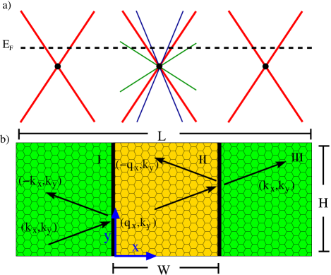
Figure 1: (Color online). a) Schematic diagram of the low-energy spectrum of Dirac quasi-particles when a velocity barrier is present. The three diagrams in a) show how the Fermi velocity $v_{F}$ (the slope of the Dirac cone) changes as a function of $x$. The green and blue Dirac cones correspond to $v_{F}<v_{F}^{0}$ and $v_{F}>v_{F}^{0}$ respectively. b) Setup needed to test the predicted effects. We set the Fermi velocity $v_{F}^{0}$ of the system for $x<0$ and $x>W$ to one. $v_{F}$ is the Fermi velocity for $0<x<W$, rendering the system non-homogeneous. The wave vectors used to find the transmission matrix solution of this problem are shown in black.

On the experimental front, a velocity barrier can be implemented in several ways. For example, one could stretch a small region of a graphene sheet Castro Neto et al. (2009), use super-lattices Park et al. (2008b); Gibertini et al. (2009) or vary the interactions with the medium around the graphene layer Jang et al. (2008); Bostwick et al. (2007). Here, we solve a generic problem in which the Fermi velocity has been modified to form what we call a velocity barrier. We must emphasize that our results are completely independent of the method used to modify the Fermi velocity, provided there is no gap opening in the system.

The proposed setup is shown in Fig.1, in which Dirac fermions move with a group velocity given by:

$$v_{eff}(x)=\left\{\begin{array}[]{rl}v_{F}^{0},&\mbox{Region $\bf{I}$, $x<0$}\\ v_{F},&\mbox{Region $\bf{II}$, $0<x<W$ }\\ v_{F}^{0},&\mbox{Region $\bf{III}$, $x>W$}\end{array}\right.$$

We will set $v_{F}^{0}$ to unity, thus the only relevant quantity will be $v_{F}$, the Fermi velocity inside the barrier, expressed in units of the Fermi velocity far from the barrier. $W$ is the barrier width.

In the absence of external potentials, quasi-particle excitations in graphene obey the Dirac equation Wallace (1947):

$$v_{eff}\vec{\sigma}\cdot\vec{p}\psi=E\psi$$ (1)

where $\vec{\sigma}=(\sigma_{x},\sigma_{y})$ is in standard Pauli matrix notation. For convenience, we define $\hbar=1$. This equation has a generic chiral solution around the Dirac point $\vec{K}$, which can be written (after a gauge transformation) in momentum space as:

$$\psi(\vec{k})=\frac{1}{\sqrt{2}}\pmatrix{1\cr se^{i\theta_{\bm{k}}}\cr}$$

where $\theta_{\bm{k}}=\arctan(k_{x}/k_{y})$ is the angle defined in momentum space. $s=\pm$ indicates the chirality of the solution which, for the case of graphene like structures, is associated with the current $\left(\vec{J}=ev_{F}\psi^{\dagger}\vec{\sigma}\psi\right)$ and not with the handedness of the system. Note that in the problem discussed in this paper, chirality will not play an important role and we are free to set $s=1$. We have assumed that the barrier is smooth compared with the lattice spacing of the underlying physical system, such that no $\bf{K}$ $\bf{K}^{\prime}$ valley mixing will occur.

We can write the general solution for this scattering problem in terms of the incident and reflected waves. In region $\bf{I}$ we have that:

$$\psi_{\bf{I}}(\vec{r})=\frac{1}{\sqrt{2}}\pmatrix{1\cr e^{i\phi}\cr}e^{i(k_{x}x+k_{y}y)}+\frac{r}{\sqrt{2}}\pmatrix{1\cr e^{i(\pi-\phi)}\cr}e^{i(-k_{x}x+k_{y}y)}$$

,

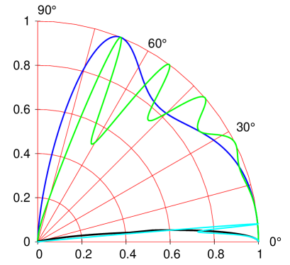
Figure 2: (Color online). Transmission probability for different values of the control parameters $E_{F}$ and $v_{F}$. Green and blue lines correspond to the case in which the effective Fermi velocity inside the barrier $0<x<W$ is $1/2$. Blue corresponds to $E_{F}$ equal to $20$ meV and green to $100$ meV. Black and cyan lines correspond to the cases in which the effective Fermi velocity inside the barrier $0<x<W$ is $10$. Black corresponds to $E_{F}$ equal to $20$ meV and cyan to $100$ meV. The barrier width is $W=350$ nm for all curves. Notice that, for large $v_{F}$, there is a critical angle (Brewster angle) for which no transmission is possible .

where $\phi=\arctan(k_{y}/k_{x})$, $k_{x}=k_{F}\cos(\phi)$, and $k_{y}=k_{F}\sin(\phi)$. In region $\bf{II}$ the solution can be constructed in a similar fashion as:

$$\psi_{\bf{II}}(\vec{r})=\frac{a}{\sqrt{2}}\pmatrix{1\cr e^{i\theta}\cr}e^{i(q_{x}x+k_{y}y)}+\frac{b}{\sqrt{2}}\pmatrix{1\cr e^{i(\pi-\theta)}\cr}e^{i(-q_{x}x+k_{y}y)}$$

, where $\theta=\arctan(k_{y}/q_{x})$, and $q_{x}=\sqrt{\left(\frac{E}{v_{F}}\right)^{2}-k_{y}^{2}}$.

For the transmitted wave we have:

$$\psi_{\bf{III}}(\vec{r})=\frac{t}{\sqrt{2}}\pmatrix{1\cr e^{i\phi}\cr}e^{i(k_{x}x+k_{y}y)}$$

Thus, in principle we have to solve the scattering problem using the transmission matrix approach. In this problem, the correct boundary conditions to be imposed at $x=0$ and $x=W$ are:

$$\psi_{\bf{I}}(0^{-}) = \sqrt{v_{F}}\psi_{\bf{II}}(0^{+})$$ (2)

$$\psi_{\bf{II}}(W^{-}) = \frac{1}{\sqrt{v_{F}}}\psi_{\bf{III}}(W^{+}).$$ (3)

These boundary conditions are a consequence of the conservation of local current at the interfaces. Solving for the coefficients $a,b,r$, and $t$, we find for the reflection coefficient:

$$r=\frac{e^{i\phi}\sin(Wq_{x})[\sin(\phi)-\sin(\theta)]}{\cos(Wq_{x})\cos(\theta)\cos(\phi)+i\sin(Wq_{x})[\sin(\theta)\sin(\phi)-1]}$$ (4)

Figs.(2) and (3) show the angular dependence of the transmission probability $T=1-|r|^{2}$. It is important to note that $T\left(\phi\right)=T\left(-\phi\right)$. Taking advantage of that symmetry, we plot our results in the interval $\phi\in[0,90^{0}]$ degrees.

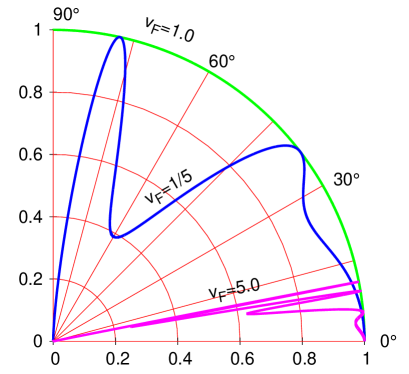
Figure 3: (Color online). Transmission probability at $E_{F}=100$ meV, $W=350$ nm and velocities inside the barrier $v_{F}=1$, $1/5$, and $5$ (green, blue, and pink lines respectively). Resonances are apparent at $Wq_{x}=n\pi$, with $n=0,1,2,...$. Note that for $v_{F}>1$ no transmission is allowed if $\phi>\phi_{cr}$.

Furthermore, for the case of massless particles at normal incidence we find that $T\left(0\right)=1$, indicating perfect transmission at normal incidence regardless of the value of $v_{F}$. The existence of peaks that reach perfect transmission at specific angles is characteristic of resonant behavior in this system. This can be readily checked by analyzing the zeros of $r$ that correspond to $\sin(Wq_{x})=0$, producing resonances at $Wq_{x}=n\pi$ for integer values of $n$ (in other words, when the barrier becomes transparent). A second peculiarity appears when $v_{F}>1$. As shown by the black and cyan lines in Fig.(2) and in pink in Fig.(3), transmission is prohibited for any angle larger than $\phi_{c}$. In Figs.(3) and (4), where we show the transmission at a fixed energy for different velocities and width ($W$), the existence of a critical angle is apparent when $v_{F}>1$. It is also clear from Fig.(2) that the only effect of increasing the energy is to increase the number of resonant peaks in $T(\phi)$. In fact, as the energy of the incident Dirac fermions is increased, more ballistic channels will be opened.

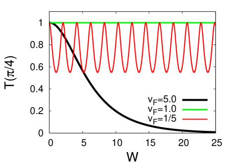
Figure 4: (Color online). Transmission probability as a function of the width $W$ for fixed energy $E_{F}=100$ meV and angle $\phi=\pi/4$. Curves in green, red, and black correspond to velocities $v_{F}=1$, $1/5$, and $5$ , respectively, inside the barrier.

The critical angle $\phi_{c}$ is analogous to the called Brewster angle in optics Landau et al. (1984). From the definition of the refracted angle:

$$\theta=\pm\arctan\left(\frac{sign\left[E_{F}\right]\sin\phi}{\sqrt{\left(\frac{1}{v_{F}}\right)^{2}-\sin^{2}\phi}}\right)$$ (5)

we can see that the critical angle will be given by $\sin^{2}\phi_{c}=v_{F}^{-2}$, which has solutions only if $v_{F}>1$, independent of $E_{F}$.

We can make a link to the standard Klein’s paradox by pointing out that Eq.(4) has the same functional form of the reflection of Dirac fermions against a potential barrier with a rectangular shape Katsnelson et al. (2006). The only difference is that the change in the Fermi velocity is encoded in the definition of $q_{x}$. This simple observation allows us to compare the effect of a velocity barrier in terms of a square potential. The dynamical variable $k_{y}$ is invariant due to the translational symmetry in the vertical direction. Therefore, it is enough to fix the second dynamical variable $q_{x}$ equal in both cases, and then solve for the potential in order to produce the same transmission coefficients in both problems. It is straightforward to show that such a potential will be:

$$V\left(E\right)=E\pm\frac{|E|}{v_{F}}$$ (6)

By using this analogy, we have obtained an energy dependent potential, which renders new phenomenology of our velocity barrier. Such energy dependent potentials have been used in nuclear physics Arellano et al. (1989), and in a different context in attempts to generalize the uncertainty principle for high energy physics Saavedra and Utreras (1981).

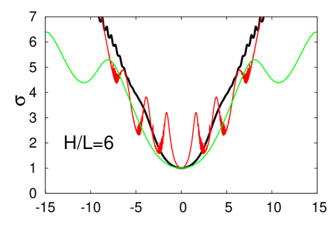
Figure 5: Conductivity $\sigma$ in units of $2e^{2}/h$ and Fano factor $F$ as a function of the energy of the incoming Dirac fermions: Green, Red, and black correspond to $v_{F}$ $5$, $0.2$, and $1.0$ respectively. $\epsilon$ is $eVH/hv_{F}$ where $V$ is the gate voltage.

We have also computed the effects of a velocity barrier on two directly measurable quantities for this system: conductivity and Fano factor DiCarlo et al. (2008); Danneau et al. (2008). In the ballistic approximation both quantities are computed using the following formulae:

$$\sigma=\left(\frac{L}{H}\right)\sum_{n=-\infty}^{\infty}T_{n},\;\;F=\frac{\sum\limits_{n=-\infty}^{\infty}T_{n}(1-T_{n})}{\sum\limits_{n=-\infty}^{\infty}T_{n}},$$ (7)

The transmission of each channel $T_{n}$ depends on a phase factor, $\alpha$, which has different values for different boundary conditions. In Fig.(5), we have used $\alpha=1/2$, corresponding to an infinite mass lateral confinement Berry and Mondragon (1987); Tworzydło et al. (2006). We have also checked that, in the wide ribbon limit, our results stay the same for other boundary conditions.

Our computation shows that $\sigma$ and $F$ are indeed sensitive to the presence of a velocity barrier. As expected from Eq.(6), the zero energy values of conductance and Fano factor remain the same. However, their values will drastically change for a small bias voltage. In Fig.(5) the red line indicates the values for $\sigma$ and $F$ for $v_{F}=1/5$, showing that conductance increases by a factor $3$ at $\epsilon\sim 1.5$, as well as large amplitude oscillations close to the Dirac point. For the case in which $v_{F}=5$ (green) few momenta can penetrate the barrier due to the existence of a Brewster angle in this case. In turn, the conductance is greatly reduced for energies away from the Dirac point. In this case, the Fano factor increases and reaches values that indicate departure from the classical diffusive limit $F=1/3$. In particular, the broad oscillation in $F$ in this case should be experimentally measurable DiCarlo et al. (2008); Danneau et al. (2008).

In this paper we have proposed a novel route to control the electric transport of massless Dirac fermions, based on experimental control Park et al. (2008b); Gibertini et al. (2009) of velocity barriers. Our main results demonstrate that it is possible, in principle, to manipulate the transmission properties of a system described by a Dirac equation by controlling the Fermi velocity. The similarity of the Fermi velocity to the role of the refractive index in optics naturally results in an effective Brewster angle, which bodes well for ultimate construction of waveguides and related devices. We have also shown that the Fano factor and the conductivity of this system can be modified by a velocity barrier, producing strong oscillations as we move away from the Dirac point. It would be interesting to produce exact simulations in order to study the precise energy window in which these effects should be observable.

This work was supported in part by the NSF under Grant No. DMR-0531159.

References

- Landau et al. (1984) L. Landau, D. Lifshitz, and L. P. Pitaevskii, Electrodynamics Of Continuous Media, vol. 8 of course of theoretical physics (Butterwort-Heinemann, London, 1984), 2nd ed.
- Arnol’d (1989) V. I. Arnol’d, Mathematical Methods of Classical Mechanics, vol. 60 (Springer-Verlag, New York, 1989), 2nd ed.
- Fetter and Walecka (1980) A. L. Fetter and J. D. Walecka, Theoretical Mechanics of Particles and Continua (McGraw-Hill, New York, 1980).
- Landau and Lifshitz (1989) L. D. Landau and E. M. Lifshitz, Mechanics, vol. 1 of Course of Theoretical Physics (Pergamon Press, Oxford, 1989), 3rd ed.
- Cheianov et al. (2007) V. V. Cheianov, V. Fal‘ko, and B. L. Altshuler, Science 315, 1252 (2007).
- Novoselov et al. (2005) K. Novoselov, A. Geim, S. Morozov, D. Jiang, M. Katsnelson, I. Grigorieva, S. Dubonos, and A. Firsov, Nature (London) 438 (2005).
- Zhang et al. (2005) Y. Zhang, Y.-W. Tan, H. L. Stormer, and P. Kim, Nature (London) 438 (2005).
- Greiner and Reinhardt (2008) W. Greiner and J. Reinhardt, Quantum electrodynamics (Springer-Verlag, Berlin, 2008), 4th ed.
- Katsnelson et al. (2006) M. I. Katsnelson, K. S. Novoselov, and A. K. Geim, Nature Phys. 2, 620 (2006).
- Shytov et al. (2008) A. V. Shytov, M. S. Rudner, and L. S. Levitov, Phys. Rev. Lett. 101, 156804 (2008).
- Young and Kim (2009) A. F. Young and P. Kim, Nature Phys. 5, 222 (2009).
- Rycerz et al. (2007) A. Rycerz, J. Tworzydlo, and C. W. J. Beenakker, Nature Phys. 3, 172 (2007).
- Nair et al. (2008) R. R. Nair, P. Blake, A. N. Grigorenko, K. S. Novoselov, T. J. Booth, T. Stauber, N. M. R. Peres, and A. K. Geim, Science 320, 1308 (2008).
- Park et al. (2008a) C.-H. Park, Y.-W. Son, L. Yang, M. L. Cohen, and S. G. Louie, Nano Lett. 8, 2920 (2008a).
- Castro Neto et al. (2009) A. H. Castro Neto, F. Guinea, N. M. R. Peres, K. S. Novoselov, and A. K. Geim, Rev. Mod. Phys. 81, 109 (2009).
- Park et al. (2008b) C.-H. Park, L. Yang, Y.-W. Son, M. L. Cohen, and S. G. Louie, Nature Phys. 4, 213 (2008b).
- Gibertini et al. (2009) M. Gibertini, A. Singha, V. Pellegrini, M. Polini, G. Vignale, A. Pinczuk, L. N. Pfeiffer, and K. W. West, Phys. Rev. B 79, 241406(R) (2009).
- Jang et al. (2008) C. Jang, S. Adam, J.-H. Chen, E. D. Williams, S. Das Sarma, and M. S. Fuhrer, Phys. Rev. Lett. 101, 146805 (2008).
- Bostwick et al. (2007) A. Bostwick, T. Ohta, T. Seyller, K. Horn, and E. Rotenberg, Nature Phys. 3, 36 (2007).
- Wallace (1947) P. R. Wallace, Phys. Rev. 71, 622 (1947).
- Arellano et al. (1989) H. F. Arellano, F. A. Brieva, and W. G. Love, Phys. Rev. Lett. 63, 605 (1989).
- Saavedra and Utreras (1981) I. Saavedra and C. Utreras, Phys. Lett. B 98, 74 (1981); H. Calisto and C. Leiva, International Journal of Modern Physics D: Gravitation, Astrophysics and Cosmology 16, 927 (2007); E. Witten, Physics Today 49, 24 (1996); A. Kempf and G. Mangano, Phys. Rev. D 55, 7909 (1997).
- DiCarlo et al. (2008) L. DiCarlo, J. R. Williams, Y. Zhang, D. T. McClure, and C. M. Marcus, Physi. Rev. Lett. 100, 156801 (2008).
- Danneau et al. (2008) R. Danneau, F. Wu, M. F. Craciun, S. Russo, M. Y. Tomi, J. Salmilehto, A. F. Morpurgo, and P. J. Hakonen, Phys. Rev. Lett. 100, 196802 (2008).
- Berry and Mondragon (1987) M. V. Berry and R. J. Mondragon, Proceedings of the Royal Society of London. A. Mathematical and Physical Sciences 412, 53 (1987).
- Tworzydło et al. (2006) J. Tworzydło, B. Trauzettel, M. Titov, A. Rycerz, and C. W. J. Beenakker, Phys. Rev. Lett. 96, 246802 (2006).