Abstract

We study the octet $SS-PP$ correlator within resonance chiral theory up to the one-loop level, i.e., up to next-to-leading order in the $1/N_{C}$ expansion. We will require that our correlator follows the power behaviour prescribed by the operator product expansion at high euclidian momentum. Nevertheless, we will not make use of short-distance constraints from other observables. Likewise, the high-energy behaviour will be demanded for the whole correlator, not for individual absorptive channels. The amplitude is progressively improved by considering more and more complicated operators in the hadronic lagrangian. Matching the resonance chiral theory result with chiral perturbation theory at low energies produces the estimates $L_{8}(\mu)^{SU(3)}=(1.0\pm 0.4)\cdot 10^{-3}$ and $C_{38}(\mu)^{SU(3)}=(8\pm 5)\cdot 10^{-6}$ for $\mu=770$ MeV. The effect of alternative renormalization schemes is also discussed in the article.

1 Introduction

The effective field theory (EFT) approach is a very powerful tool for the investigation of Quantum Chromodynamics (QCD) at long distances. Chiral Perturbation theory ($\chi$PT) [1, 2, 3] is the EFT for the description of the chiral (pseudo) Goldstones in the low energy domain $p^{2}\ll\Lambda_{H}^{2}\sim 1$ GeV², with $\Lambda_{H}$ typically the scale of the lowest resonance masses. The calculation of the QCD matrix elements is then organized at long distances in growing powers of the external momenta and light quark masses. Recent progress has allowed to carry $\chi$PT up to ${\cal O}(p^{6})$, i.e., up to the two-loop level [4, 5, 6, 7].

In the intermediate resonance region, $\Lambda_{H}\stackrel{{\scriptstyle<}}{{{}_{\sim}}}E\stackrel{{\scriptstyle<}}{{{}_{\sim}}}2$ GeV, $\chi$PT stops being valid and one must explicitly include the resonance fields in the Lagrangian description. Unfortunately, this is not a straightforward process because there is no natural expansion parameter in this region as several relevant mass scales appear in this range (resonance masses, momenta, widths, the characteristic $\chi$PT loop scale $\Lambda_{\chi}\sim 4\pi F$…). Resonance Chiral Theory (R$\chi$T) describes the interaction of resonance and pseudo-Goldstones within a general chiral invariant framework [8, 9]. Alternatively to the chiral counting, it uses the $1/N_{C}$ expansion of QCD in the limit of large number of colours [10] as a guideline to organize the perturbative expansion. At leading order (LO), just tree-level diagrams contribute while loop diagrams yield higher order effects. Integrating out the heavy resonance states leaves at low energies the corresponding chiral invariant effective theory, $\chi$PT. Many works have investigated various aspects of R$\chi$T: equivalence of formalisms [9, 11, 12, 13]; Green functions [14, 15, 16, 17, 18, 19, 20]; applications to phenomenology [14, 21, 22, 23, 24, 25, 26, 27]; determination of chiral low-energy constants (LECs) at NLO in $1/N_{C}$ [21, 29, 30, 31, 32]; determination of the one-loop ultraviolet divergence structures in the generating functional [33]; implications about the renormalizability [34, 35]; possible issues with extra degrees of freedom in the renormalized propagator [36, 37]; renormalization group studies [38].

The infinite tower of mesons contained in large–$N_{C}$ QCD is often truncated to the lowest states in each channel, usually named as single resonance approximation (SRA). This approximation has led to successful predictions of ${\cal O}(p^{4})$ and ${\cal O}(p^{6})$ low-energy constants (LECs) [8, 9, 21, 28, 39]. However, the study of Regge models with an infinite number of mesons has shown that if one keeps just the lightest states with exactly the same couplings and masses of the full model then one finds problems in the short-distance matching and wrong values are obtained for the LECs [40]. Thus, in a high-energy matching with the operator product expansion (OPE) [41] the parameters of the truncated theory will be shifted in order to accommodate the right short-distance dependence. Chiral symmetry ensures the proper low-momentum structure of the R$\chi$T amplitudes around $p^{2}=0$ but their high energy behaviour is not fixed by symmetry alone. In that sense, the matched amplitude can be understood with the help of Padé approximants as an rational interpolator between the deep Euclidean $p^{2}=-\infty$ and $p^{2}=0$ [43, 44]. The Weinberg sum-rules (WSR) [42] yield the most convenient parameters for the interpolation rather than the accurate determinations of the resonance couplings. Furthermore, the R$\chi$T couplings for the lightest mesons are expected to be in better agreement, whereas the parameters from the highest excitations may lie far from their right values [43].

The connection of the R$\chi$T amplitudes with the operator product expansion (OPE) at high energies seems a priori a useful procedure to include extra information from QCD in the resonance theory. It allows to fix combinations of couplings (e.g., through WSR), decreasing the number of unknown parameters in the analysis. However, large–$N_{C}$ QCD has an infinite number of hadrons and in order to reproduce the full large–$N_{C}$ theory one must consider the tree-level exchanges of heavier and heavier resonances. In the hadronical ansatz approach, one adds more and more poles to the rational approximant [43, 44]. Equivalently, this can be realized within the quantum field theory framework as a generating functional with a lagrangian including interaction operators $J-R_{j}$ that couple the external current source $J$ and heavier and heavier resonances $R_{j}$ (e.g. of the form $c_{m,j}\langle\,S_{j}\chi_{+}\,\rangle$ for the $SS$ correlator).

The extension of R$\chi$T beyond the tree level approximation still needs to be worked out in detail. Although some theoretical issues on the renormalizability of R$\chi$T still need further clarification [34, 35, 45], several chiral LECs have been already computed up to NLO in $1/N_{C}$ through quantum field theory (QFT) one-loop calculations [29, 30] and dispersion relations [31, 32]. In this article we will focus our attention on the chiral octet $SS-PP$ correlator (for instance, with $I=1$), which in the chiral limit is determined at low energies by the ${\cal O}(p^{4})$ and ${\cal O}(p^{6})$ LECs, respectively, by $L_{8}$ [3] and $C_{38}$ [4]. The correlator is computed up to next-to-leading order in $1/N_{C}$ (NLO) and the chiral limit will be assumed all along the article.

At the one-loop level –NLO in $1/N_{C}$–, one needs also to devise a procedure to reach the infinite resonance limit of large–$N_{C}$ QCD. In the case of two–point Green-functions, the imaginary part of the one-loop diagrams is given through the optical theorem by the square of two-meson form-factors computed at tree-level. Thus, based on a dispersive approach, one may add the contribution to the spectral function from higher and higher two-meson absorptive cuts by providing the corresponding form-factors [31, 32]. This would be, in some sense, the natural extension of the minimal hadronical ansatz [44] to the one-loop situation. In a previous computation of the octet $SS-PP$ correlator up to NLO in $1/N_{C}$, the intermediate two-meson channels were analyzed individually [31]. The corresponding tree-level form-factors were made to vanish appropriately at high energies [32, 46]. This allowed to recover the correlator from its spectral function through an unsubtracted dispersion relation. However, in general, it is not always possible to fulfill the high-energy constraints for all the form-factors at once . Only the two-meson absorptive cuts with at most one resonance ($\pi\pi$ and $R\pi$) were considered in Ref. [31], as the $RR^{\prime}$ channels have their thresholds at $(M_{R}+M_{R^{\prime}})\sim 2$ GeV and are suppressed at low energies. Likewise, the short-distance constraints from $VV-AA$ Weinberg sum-rules and the $\pi\pi$ vector and the scalar form-factor were used there in order to fix some of the couplings appearing in the analysis.

In the quantum field theory approach proposed in this work, one has a mesonic lagrangian which at the classical level generates the large–$N_{C}$ amplitudes and whose quadratic fluctuations around the classical field configuration provide the one-loop corrections [33]. The complete QCD generating functional is approached as one adds more and more hadronic operators to the action. Eventually, one should add the infinite number of possible terms of the given $1/N_{C}$ order under consideration. For instance, the $S\pi\pi$ interaction (provided by $c_{d}\langle\,Su_{\mu}u^{\mu}\,\rangle$ [8]) is of the same order as in $1/N_{C}$ as the $SP\pi$ vertex (given by the $\lambda_{1}^{SP}\langle\,\{\nabla^{\mu}S,P\}u_{\mu}\,\rangle$ operator [15, 32, 46]). Notice that one never has a complete description with a finite number of operators. The basic lagrangian $\mathcal{L}_{G}+\mathcal{L}_{R}$ with at most one resonance field in each term [8] provides an incomplete description of the $R\pi$ channels, as the possible diagrams with $R^{\prime}$ resonances exchanged in the $s$–channel are missing [31, 32]. This requires the incorporation of operators $\mathcal{L}_{RR^{\prime}}$ with two resonance fields [15, 32, 46]. In the same way, the $RR^{\prime}$ absorptive cuts are now badly described without the $\mathcal{L}_{RR^{\prime}R^{\prime\prime}}$ terms with three resonance fields.

The chiral structure of the lagrangian ensures the right structure at long distances. On the other hand, we will impose that the correlator follows the short-distance behaviour prescribed by the OPE. The one-loop R$\chi$T amplitude will be used as an improved interpolator between low and high energies. The resonance couplings become then interpolating parameters that must approach their actual values in the full QCD as more and more operators are added to the R$\chi$T action. On the contrary to what was done in former works [31, 32], the short-distance matching will be carried out in the present article for the total correlator and spectral function [47], rather than for individual channels. Likewise, we will not use the short-distance constraints from other amplitudes to fix the couplings in the one-loop correlator. We will work within the SRA, including just the chiral Goldstones and the lightest multiplets of scalar, pseudo-scalar, vector and axial-vector resonances. In a first step, the $SS-PP$ correlator will be computed at NLO in $1/N_{C}$ with the simplest R$\chi$T lagrangian, with operators with at most one resonance field ($G_{V}$, $c_{m}$, $d_{m}$…) [8]. This provides the proper structure for the intermediate tree-level exchanges ($\pi,\,S,\,P$ one-particle channels) and the two-Goldstone cut $\pi\pi$. However, this simple lagrangian fails to describe the $R\pi$ and $RR^{\prime}$ channels as the lagrangian [8] makes their form-factors behave like a constant or like a growing power of the momentum at high energies [30, 31, 32, 46, 48]. This will be partly cured by the consideration of $\lambda^{RR^{\prime}}$ operators with two resonance fields [15, 32, 46, 48], which now allow an appropriate description of the $R\pi$ channels, though the $RR^{\prime}$ ones still behave badly. Although these cuts with two resonances were neglected in the dispersive approach [31], removing part of the one-loop diagrams is not theoretically well defined and may lead to inconsistences in the renormalization of the QFT. Furthermore, it is not trivial that the effect of the $RR^{\prime}$ cuts in the short-distance matching is fully negligible. Hence, all the possible diagrams contributing to the correlator up to NLO will be kept in our study.

The amplitude is first computed within the usual subtraction scheme of $\chi$PT [2] (denoted for simplicity as $\widetilde{MS}$ all along the article). However, though equivalent at low energies, some appropriate schemes will be found more convenient: pole masses and other schemes that minimize the uncertainties derived from the short-distance constraints. This will help us to determine the ${\cal O}(p^{4})$ and ${\cal O}(p^{6})$ LECs, respectively $L_{8}(\mu)$ and $C_{38}(\mu)$. The high-energy constraints and their meaning will be discussed and the convergence to full large–$N_{C}$ QCD will be tested as more and more hadronic operators are added to the R$\chi$T  action. This work is thought as a complementary and an alternative approach to the dispersive analysis in Ref. [31].

The article is organized as follows. Resonance chiral theory is introduced in detail in Sec. 2. The octet $SS-PP$ correlator is defined in Sec. 3 and its one-loop R$\chi$T computation is provided in Sec. 4. The high-energy constraints and low energy expansions are respectively given in Secs. 5 and 6. The contributions from operators $\mathcal{L}_{RR^{\prime}}$ with two resonance fields have been singled out in Sec. 7 to ease the main argumentation of the article. Finally, the phenomenological analysis is given in Sec. 8 and the conclusions are provided in Sec. 9. Some technical results are relegated to the Appendices.

2 Resonance chiral theory lagrangian

Within the large–$N_{C}$ approach the mesons will be classified within $U(3)$ multiplets. The chiral Goldstone bosons are introduced by means of the basic building block,

$$u(\phi)=\exp\left(i\frac{\phi}{\sqrt{2}F}\right)$$ (1)

where $\phi=\frac{1}{\sqrt{2}}\lambda^{a}\phi^{a}$ and

$$\phi(x)\,\,=\,\,\left(\begin{array}[]{ccc}\frac{1}{\sqrt{2}}\pi^{0}+\frac{1}{\sqrt{6}}\eta_{8}+\frac{1}{\sqrt{3}}\eta_{1}&\pi^{+}&K^{+}\\ \pi^{-}&-\frac{1}{\sqrt{2}}\pi^{0}+\frac{1}{\sqrt{6}}\eta_{8}+\frac{1}{\sqrt{3}}\eta_{1}&K^{0}\\ K^{-}&\overline{K}^{0}&-\frac{2}{\sqrt{6}}\eta_{8}+\frac{1}{\sqrt{3}}\eta_{1}\\ \end{array}\right)\,.$$ (2)

This forms the basic covariant tensors,

$$u_{\mu} = i\,\{u^{\dagger}(\partial_{\mu}-ir_{\mu})u\,-\,u\,(\partial_{\mu}-i\ell_{\mu})u^{\dagger}\}\,,$$

$$\chi_{\pm} = u^{\dagger}\,\chi\,u^{\dagger}\,\pm\,u\,\chi^{\dagger}\,u\,,$$ (3)

$$f_{\pm}^{\mu\nu} = u\,F_{L}^{\mu\nu}\,u^{\dagger}\,\pm\,u^{\dagger}\,F_{R}^{\mu\nu}\,u\,,$$

with $\chi=2B_{0}(s+ip)$ containing the scalar and pseudo-scalar external sources, $s$ and $p$ respectively, the right and left sources $r^{\mu}$ and $\ell^{\mu}$ providing the vector and axial-vector external sources, $v^{\mu}=\frac{1}{2}(r^{\mu}+\ell^{\mu})$ and $a^{\mu}=\frac{1}{2}(r^{\mu}-\ell^{\mu})$ respectively, and $F_{L,R}^{\mu\nu}$ the corresponding left and right field-strength tensors.

The Goldstone bosons are parametrized by the elements $u(\phi)$ of the coset space $U(3)_{L}\times U(3)_{R}/U(3)_{V}$, transforming as

$$u(\phi)\mapsto V_{R}u(\phi)h(g,\phi)^{-1}=h(g,\phi)u(\phi)V_{R}$$ (4)

under a general chiral rotation $g=(V_{L},V_{R})\subset G$ in terms of the $U(3)_{V}$ compensator field $h(g,\phi)$. This makes the tensors $X=u^{\mu},\chi_{\pm},f_{\pm}^{\mu\nu}$ to transform covariantly in the form,

$$X\,\mapsto\,h(g,\phi)\,X\,h(g,\phi)^{-1}\,.$$ (5)

2.1 Leading order lagrangian

For the classification of the vertices entering in the tree-level and one-loop amplitudes it will be useful to organize the operators of the R$\chi$T lagrangian according to the number of resonance fields:

$$\mathcal{L}\,\,=\,\,\mathcal{L}_{G}\,\,+\,\mathcal{L}_{R}\,\,+\,\,\mathcal{L}_{RR^{\prime}}\,\,+\,\,\ ...$$ (6)

where $\mathcal{L}_{G}$ only contains Goldstone bosons and external sources, $\mathcal{L}_{R}$ also includes one resonance, etc. Although in principle one should consider all the terms compatible with symmetry, most of the large–$N_{C}$ phenomenological calculations consider operators with the minimal number of derivatives [39]. This is usually justified through the argument that higher derivative operators tend to violate the asymptotic high energy QCD behaviour [9, 39]. Likewise, its has been proven in several cases that higher derivative resonance operators can be removed from the hadronic action through meson field redefinitions in the generating functional [30, 33, 34, 35, 46, 48]. In the present article, the leading lagrangian will only contain operators at most ${\cal O}(p^{2})$, with the external sources counted as $v^{\mu},a^{\mu}\sim{\cal O}(p)$ and $\chi\sim{\cal O}(p^{2})$ [46, 47].

The Lagrangian with only Goldstones has the same form as in $\chi$PT but the coupling constants are different. In $\chi$PT we have the leading order Lagrangian

$${\cal L}_{\rm\chi PT}^{(2)}=\frac{F^{2}}{4}\langle u_{\mu}u^{\mu}+\chi_{+}\rangle\,.$$ (7)

In R$\chi$T beyond leading order the constants standing in front of the operators $\langle\,u^{\mu}u_{\mu}\,\rangle$ and $\langle\,\chi_{+}\,\rangle$ may not be the same as in $\chi$PT. Therefore, generally we can write

$${\cal L}_{G}=\frac{\widetilde{F}^{2}}{4}\langle u^{\mu}u_{\mu}\rangle+\frac{\hat{F}^{2}}{4}\langle\chi_{+}\rangle$$ (8)

where we explicitly distinguish between $\widetilde{F}$ and $\hat{F}$. These can be split in the way,

$$\widetilde{F}=F+\delta\widetilde{F},\qquad\hat{F}=F+\delta\hat{F}$$ (9)

where at large $N_{C}$ one has the matching condition $\widetilde{F}=\hat{F}=F$ and, hence, $\delta\widetilde{F}$ and $\delta\hat{F}$ are NLO in $1/N_{C}$. On the contrary to what happens in $\chi$PT, where the parameters ($F$ and $B_{0}$) which characterize the terms $\langle\,u^{\mu}u_{\mu}\,\rangle$ and $\langle\,\chi_{+}\,\rangle$ do not become renormalized, in R$\chi$T the couplings of these two operators are needed to make the physical amplitude finite. For simplicity, we choose to keep the definitions of the chiral tensors unchanged and to renormalize instead $\widetilde{F}$ and $\hat{F}$, as it was done in Refs. [33, 46] with the notation $\alpha_{1}=\widetilde{F}^{2}/4$ and $\alpha_{2}=\hat{F}^{2}/4$.

The Goldstone bosons couple to massive $U(3)$ multiplets of the type $V(1^{--})$, $A(1^{++})$, $S(0^{++})$ and $P(0^{-+})$. The vector multiplet, for instance, is given by

$$V_{\mu\nu}\,\,=\,\,\left(\begin{array}[]{ccc}\frac{1}{\sqrt{2}}\rho^{0}+\frac{1}{\sqrt{6}}\omega_{8}+\frac{1}{\sqrt{3}}\omega_{1}&\rho^{+}&K^{*\,+}\\ \rho^{-}&-\frac{1}{\sqrt{2}}\rho^{0}+\frac{1}{\sqrt{6}}\omega_{8}+\frac{1}{\sqrt{3}}\omega_{1}&K^{*\,0}\\ K^{*\,-}&\overline{K}^{\,*\,0}&-\frac{2}{\sqrt{6}}\omega_{8}+\frac{1}{\sqrt{3}}\omega_{1}\\ \end{array}\right)_{\mu\nu}\,,$$ (10)

where we use the antisymmetric tensor formalism for spin–1 fields to describe the vector and axial-vector resonances [8, 9, 13].

The resonance fields $R$ are chosen to transform covariantly under the chiral group as in Eq. (5) [8]. The free-field kinetic term is given by the operators

$${\cal L}_{RR}^{\rm Kin}\,\,=\,\,-\frac{1}{2}\langle\nabla^{\mu}R_{\mu\nu}\nabla_{\alpha}R^{\alpha\nu}\rangle+\frac{1}{4}M_{R}^{2}\langle R_{\mu\nu}R^{\mu\nu}\rangle+\frac{1}{2}\langle\nabla^{\alpha}R^{\prime}\nabla_{\alpha}R^{\prime}\rangle-\frac{1}{2}M_{R^{\prime}}^{2}\langle R^{\prime}R^{\prime}\rangle\,.$$ (11)

where $R=V,A$ are vector and axial vector resonances and $R^{\prime}=S,P$ are scalar and pseudoscalar resonances.

The interaction terms which are linear in the resonance fields can be obtained from the seminal work [8]:

$${\cal L}_{R} = c_{d}\langle Su^{\mu}u_{\mu}\rangle+c_{m}\langle S\chi_{+}\rangle+id_{m}\langle P\chi_{-}\rangle+\frac{F_{V}}{2\sqrt{2}}\langle V_{\mu\nu}f_{+}^{\mu\nu}\rangle+\frac{iG_{V}}{2\sqrt{2}}\langle V_{\mu\nu}[u^{\mu},u^{\nu}]\rangle+\frac{F_{A}}{2\sqrt{2}}\langle A_{\mu\nu}f_{-}^{\mu\nu}\rangle.$$

For our analysis of the $SS-PP$ correlator, the relevant bilinear terms will be [15, 46, 48]

$$\mathcal{L}_{RR^{\prime}}\,=\,i\lambda_{1}^{PV}\langle\,[\nabla^{\mu}P,V_{\mu\nu}]\,u^{\nu}\,\rangle\,+\,\lambda_{1}^{SA}\langle\,\{\nabla^{\mu}S,A_{\mu\nu}\}\,u^{\nu}\,\rangle\,+\,\lambda_{1}^{SP}\langle\,\{\nabla^{\mu}S,P\}\,u_{\mu}\,\rangle\,.$$ (13)

Only single flavor–trace operators are considered for the construction of the large–$N_{C}$ lagrangian. At tree-level, the octet $SS-PP$ correlator only gets contributions from this kind of terms, even at subleading orders in $1/N_{C}$. Operators with two or more traces might appear in the vertices of one loop diagrams but, since these multi-trace terms are $1/N_{C}$–suppressed, these contributions would go to next-to-next-to-leading order and they will be neglected in the present work.

The previous operators provide an appropriate description of the form factors with two Goldstones or one resonance and one Goldstone in the final state. We will perform our most elaborate analysis with the lagrangian $\mathcal{L}_{G}+\mathcal{L}_{R}+\mathcal{L}_{RR^{\prime}}$, with at most two resonance fields. As we will see in next sections, the R$\chi$T description will progressively approach the actual QCD amplitude as more and more complicated operators are added. However, although we expect the contributions from the operators with three resonance fields to the LECs to be negligible at our level of accuracy, a further refinement is eventually possible by considering these operators $\mathcal{L}_{RR^{\prime}R^{\prime\prime}}$ .

2.2 Subleading Lagrangian

At the loop level, one needs to introduce new subleading operators in order to cancel the ultraviolet divergences, to renormalize R$\chi$T and to make the amplitudes finite. As the leading order lagrangian operators are ${\cal O}(p^{2})$, the naive dimensional analysis tells us that at one loop one expects to find ${\cal O}(p^{4})$ ultraviolet divergences, requiring the introduction of NLO counter-terms with a higher number of derivatives.

The new operators with just Goldstone bosons required at NLO are, for the $SS-PP$ correlator under consideration,

$${\cal L}_{GB}^{NLO} = \frac{\widetilde{L}_{8}}{2}\langle\chi_{-}^{2}+\chi_{+}^{2}\rangle+i\widetilde{L}_{11}\langle\chi_{-}(\nabla_{\mu}u^{\mu}-\frac{i}{2}\chi_{-})\rangle-\widetilde{L}_{12}\langle(\nabla_{\mu}u^{\mu}-\frac{i}{2}\chi_{-})^{2}\rangle+\frac{\displaystyle\widetilde{H}_{2}}{\displaystyle 4}\langle\chi_{+}^{2}-\chi_{-}^{2}\rangle\,.$$

Though we use the same structure of terms as in $\chi$PT, the R$\chi$T couplings $\widetilde{L}_{i}$ are not the same as the chiral LECs $L_{i}$. The $\widetilde{L}_{i}$ will contribute at low energies to ${\cal O}(p^{4})$ chiral couplings $L_{i}$. The latter are dominantly saturated by resonances exchanges, so $\widetilde{L}_{i}$ are considered to be suppressed and subleading in the $1/N_{C}$ expansion.

In order to make the resonance propagator finite, one needs to renormalize the mass and wave functions ($M_{R}^{(B)\,\,2}=M_{R}^{r\,\,2}+\delta M_{R}^{2}$, $R^{(B)}=Z_{R}^{\frac{1}{2}}R^{r}$) and to introduce at NLO in $1/N_{C}$ the kinetic operator

$${\cal L}_{\rm Kin}^{NLO}\,\,=\,\,\frac{\displaystyle X_{R}}{\displaystyle 2}\langle R\nabla^{4}R\rangle\,,$$ (15)

with $R=S,P$. No terms with vector or axial-vectors are needed for the present NLO analysis of the $SS-PP$ correlator.

Likewise, the renormalization of the vertex functions $s(x)\to S$ and $p(x)\to P$ at NLO in $1/N_{C}$ will require of the linear terms,

$${\cal L}_{R}^{NLO} = \lambda^{S}_{18}\langle S\nabla^{2}\chi_{+}\rangle\,\,+\,\,i\lambda^{P}_{13}\langle P\nabla^{2}\chi_{-}\rangle\,.$$ (16)

At NLO in $1/N_{C}$, all these subleading counter-terms can only contribute through tree-level diagrams.

2.3 Equations of motion and redundant operators

The equations of motion (EOM) of the leading lagrangian are given by [46, 33],

$$\nabla^{\mu}u_{\mu} = \frac{\displaystyle i}{\displaystyle 2}\chi_{-}+\frac{\displaystyle ic_{m}}{\displaystyle F^{2}}\{\chi_{-},S\}-\frac{\displaystyle d_{m}}{\displaystyle F^{2}}\{\chi_{+},P\}\,\,\,+\,\,\,...$$ (17)

$$\nabla^{2}S = -M_{S}^{2}S+c_{d}u_{\mu}u^{\mu}+c_{m}\chi_{+}\,\,\,+\,\,\,...$$ (18)

$$\nabla^{2}P = -M_{P}^{2}P+id_{m}\chi_{-}\,\,\,+\,\,\,...$$ (19)

where the dots stand for terms with vector or axial-vector resonances or sources, two-meson fields or with one scalar-pseudoscalar external source and one meson field.

Since most of the subleading resonance operators are proportional to the EOM, it is possible to simplify our new NLO resonance operators by means of appropriate meson field redefinitions,:

$$\mathcal{L}_{\rm Kin}^{NLO}\longrightarrow{\cal L}^{NLO,\,\,eff}_{{\rm Kin}} = -\lambda^{S}_{18}M_{S}^{2}\langle SS\rangle+c_{m}\lambda^{S}_{18}\langle\chi_{+}^{2}\rangle-i\lambda^{P}_{13}M_{P}^{2}\langle PP\rangle-d_{m}\lambda^{P}_{13}\langle\chi_{-}^{2}\rangle\,\,\,+\,\,\,...$$

$$\mathcal{L}_{R}^{NLO}\longrightarrow{\cal L}_{R}^{NLO,\,\,eff} = \frac{X_{S}M_{S}^{4}}{2}\langle SS\rangle+\frac{c_{m}^{2}X_{S}}{2}\langle\chi_{+}^{2}\rangle-c_{m}X_{S}M_{S}^{2}\langle S\chi_{+}\rangle$$ (20)

$$+\frac{X_{P}M_{P}^{4}}{2}\langle PP\rangle-\frac{d_{m}^{2}X_{P}}{2}\langle\chi_{-}^{2}\rangle-id_{m}X_{P}M_{P}^{2}\langle P\chi_{-}\rangle\,\,\,+\,\,\,...$$

where the dots stand for operators that do not contribute to the $SS-PP$ correlator at NLO. After the field redefinition the resonance operators $\mathcal{L}_{\rm Kin}^{NLO}$ and $\mathcal{L}_{R}^{NLO}$ disappear and the surviving terms in the R$\chi$T lagrangian carry in front the effective combinations,

$$\widetilde{L}_{8}^{eff} = \widetilde{L}_{8}+\frac{1}{2}c_{m}^{2}X_{S}-\frac{1}{2}d_{m}^{2}X_{P}+c_{m}\lambda^{S}_{18}-d_{m}\lambda^{P}_{13},$$

$$\widetilde{H}_{2}^{eff} = \widetilde{H}_{2}+c_{m}^{2}X_{S}+d_{m}^{2}X_{P}+2c_{m}\lambda^{S}_{18}+2d_{m}\lambda^{P}_{13},$$

$$(M_{S}^{2})^{eff} = M_{S}^{2}-X_{S}M_{S}^{4},$$

$$(M_{P}^{2})^{eff} = M_{P}^{2}-X_{P}M_{P}^{4},$$

$$c_{m}^{eff} = c_{m}-c_{m}X_{S}M_{S}^{2}-M_{S}^{2}\lambda^{S}_{18},$$

$$d_{m}^{eff} = d_{m}-d_{m}X_{P}M_{P}^{2}-M_{P}^{2}\lambda^{P}_{13}.$$ (21)

The $\widetilde{L}_{11}$ and $\widetilde{L}_{12}$ operators do not contribute to terms which can be relevant to our amplitude up to NLO and we will see that they are not present in the final result.

3 Chiral octet $SS-PP$ correlator

In the case of $SU(3)$–octet quark bilinears, the two-point Green function $SS-PP$ is defined as

$$\Pi_{S-P}^{ab}(p)\,\,=\,\,i\,\int d^{4}xe^{ip\cdot x}\langle 0|T[S^{a}(x)S^{b}(0)-P^{a}(x)P^{b}(0)]|0\rangle=\delta^{ab}\Pi(p^{2})\,,$$ (22)

with $S^{a}=\bar{q}\frac{\lambda_{a}}{\sqrt{2}}q$ and $P^{a}=i\bar{q}\frac{\lambda_{a}}{\sqrt{2}}\gamma_{5}q$, being $\lambda_{a}$ the Gellmann matrices ($a=1,\dots 8$).

In the chiral limit, assumed all along the article, the low-energy expansion of the octet correlators is determined by $\chi$PT in the form [5],

$$\Pi(p^{2})_{\chi PT} = B_{0}^{2}\Bigg{\{}\frac{2F^{2}}{p^{2}}+\left[32L^{r}_{8}(\mu_{\chi})+\frac{\Gamma_{8}}{\pi^{2}}\left(1-\ln\frac{-p^{2}}{\mu_{\chi}^{2}}\right)\right]$$

$$\hskip 28.45274pt+\frac{p^{2}}{F^{2}}\left[32C_{38}^{r}(\mu_{\chi})-\frac{\Gamma^{(L)}_{38}}{\pi^{2}}\left(1-\ln\frac{-p^{2}}{\mu_{\chi}^{2}}\right)+{\cal O}(N_{C}^{0})\right]+{\cal O}(p^{4})\Bigg{\}}$$

where in $\Gamma_{8}=5/48$ [$3/16$] and $\Gamma^{L}_{38}=-5L_{5}/6$ [$-3L_{5}/2$] in $SU(3)$–$\chi$PT [$U(3)$–$\chi$PT]. Notice that in $\chi$PT the correlator is exactly independent of the renormalization scale $\mu_{\chi}$, being its choice completely arbitrary.

In the resonance region, one obtains at leading order in $1/N_{C}$,

$$\Pi(p^{2})_{LO}\,=\,\frac{2B_{0}^{2}F^{2}}{p^{2}}\,+\,16B_{0}^{2}\sum_{i}\left(\frac{c_{m,i}^{2}}{M_{S,i}^{2}-p^{2}}\,-\,\frac{d_{m,i}^{2}}{M_{P,i}^{2}-p^{2}}\right)\,,$$ (24)

where one sums over the different resonance multiplets. The subscript _,i in $M_{R,i}$, $c_{m,i}$ and $d_{m,i}$ refers to the coupling of the $i$–th resonance multiplet of the corresponding kind. The requirement of the high energy OPE behaviour $\Pi(p^{2})\stackrel{{\scriptstyle p^{2}\rightarrow\infty}}{{\sim}}1/p^{6}$ produces the short-distance conditions   [39]

$$\sum_{i}(c_{m,i}^{2}-d_{m,i}^{2})=\frac{F^{2}}{8},\qquad\qquad\sum_{i}c_{m,i}^{2}M_{S,i}^{2}-d_{m,i}^{2}M_{P,i}^{2}=0\,.$$ (25)

In the single resonance approximation (SRA), it is then possible to express $c_{m}$ and $d_{m}$ in terms of $F$ and resonance masses,

$$c_{m}^{2}\,\,=\,\,\frac{F^{2}}{8}\,\frac{M_{P}^{2}}{M_{P}^{2}-M_{S}^{2}}\qquad\qquad\qquad d_{m}^{2}\,\,=\,\,\frac{F^{2}}{8}\,\frac{M_{S}^{2}}{M_{P}^{2}-M_{S}^{2}}.$$ (26)

At low energies, we can match the large–$N_{C}$ expression (24) with the $\chi$PT expression (3), obtaining the LO prediction for the low energy coupling constants $L_{8}$ and $C_{38}$,

$$L_{8} = \frac{c_{m}^{2}}{2M_{S}^{2}}-\frac{d_{m}^{2}}{2M_{P}^{2}}=\frac{F^{2}}{16}\left(\frac{1}{M_{P}^{2}}+\frac{1}{M_{S}^{2}}\right),$$ (27)

$$C_{38} = \frac{c_{m}^{2}F^{2}}{2M_{S}^{4}}-\frac{d_{m}^{2}F^{2}}{2M_{P}^{4}}=\frac{F^{4}}{16M_{P}^{2}M_{S}^{2}}\left(1+\frac{M_{P}^{2}}{M_{S}^{2}}+\frac{M_{S}^{2}}{M_{P}^{2}}\right)$$ (28)

For the inputs $M_{S}=M_{P}/\sqrt{2}\simeq 1$ GeV, one obtains $L_{8}\approx 0.7\cdot 10^{-3}$, $C_{38}\approx 7\cdot 10^{-6}$ for $M_{S}=1\,{\rm GeV}$. However, one does not know to what renormalization scale $\mu_{\chi}$ these numerical predictions correspond. In order to pin down this $\mu$–dependence, one must carry the calculation up to the loop level.

4 One-loop computation in resonance chiral theory

We follow the renormalization procedure presented in [30]. In general, we will use dimensional regularization and the ${\overline{MS}}-1$ subtraction scheme, usually employed in $\chi$PT calculations [2, 3]. This means we will absorb in the coupling counter-terms the ultraviolet divergent piece from the loops, counter-terms,

$$\lambda_{\infty}(\mu)\,\,=\,\,\mu^{d-4}\,\left[\frac{2}{d-4}\,+\,\gamma_{E}\,-\,\ln 4\pi\,-\,1\,\right]\,.$$ (29)

Still, the Goldstone propagator and the Goldstone decay amplitudes will be renormalized in the on-shell scheme, as it is done in $\chi$PT, in order to ease the low-energy matching of R$\chi$T and $\chi$PT at ${\cal O}(p^{2})$. Everything else will be renormalized in this section in $\overline{MS}-1$. For simplicity, we will denote this set of schemes as $\widetilde{MS}$ from now on. Afterwards, we will study alternative renormalization schemes for the R$\chi$T couplings and their relation with the $\widetilde{MS}$ parameters.

In this section, together with the general structure of the amplitudes, we will provide in this Section just the explicit results for the case when the lagrangian contains the operators $\mathcal{L}_{G}+\mathcal{L}_{R}$ with at most one resonance field, derived by Ecker et al. [8]. The contributions from operators $\mathcal{L}_{RR^{\prime}}$ with two resonance fields are provided separately later in Sec. 7. For clarity, we provide the individual contributions from each absorptive cut (e.g. $\pi\pi$, $V\pi$…). The precise definitions for the corresponding Feynman integrals are given in Appendix C.

4.1 Goldstone boson renormalizations

4.1.1 Goldstone self-energy

Figure 1: Contributions to the Goldstone boson self-energy. The single line represents the Goldstone boson while the double line represents the resonance. The type of resonance is written above it.

The general form of the renormalized Goldstone propagator is given by

$$i\Delta_{\phi}^{-1}\,\,=\,\,\frac{\widetilde{F}^{2}\,Z_{\phi}}{F^{2}}p^{2}\,\,-\,\,\frac{4\widetilde{L}_{12}p^{4}}{F^{2}}\,\,-\,\,\Sigma_{\phi}(p^{2})\,,$$ (30)

with $Z_{\phi}$ the wave function renormalization of the bare Goldstone field, $\phi^{(B)}=Z_{\phi}^{\frac{1}{2}}\phi^{r}$. In order to make the propagator finite, one needs to perform the shifts

$$Z_{\phi}=1+\delta Z_{\phi},\qquad\widetilde{F}=F+\delta\widetilde{F},\qquad\widetilde{L}_{12}=\widetilde{L}_{12}^{r}+\delta\widetilde{L}_{12}\,,$$ (31)

where $\delta Z_{\phi}$ and $\delta\widetilde{F}$ are NLO in $1/N_{C}$. The NLO coupling $\widetilde{L}_{12}$ is split into a finite renormalized part $\widetilde{L}^{r}_{12}$ and an infinite counter-term $\delta\widetilde{L}_{12}$.

Considering the on-shell renormalization scheme for the Goldstone propagator, i.e. such that $i\Delta^{-1}_{\phi}=p^{2}+{\cal O}(p^{4})$, leads to the renormalization condition

$$\frac{2\delta\widetilde{F}}{F}\,+\,\delta Z_{\phi}\,-\,\Sigma_{\phi}^{\,{}^{\prime}}(0)\,\,=\,\,0\,,$$ (32)

with $\Sigma_{\phi}^{\,{}^{\prime}}(0)=\left.\frac{\displaystyle d\Sigma_{\phi}}{\displaystyle dp^{2}}\right|_{p^{2}=0}$. The ${\cal O}(p^{4})$ ultraviolet divergence in $\Sigma_{\phi}$ is absorbed into $\delta\widetilde{L}_{12}$ in the $\widetilde{MS}$ scheme. The renormalized Goldstone propagator is then provided by

$$i\Delta_{\phi}^{-1}=p^{2}\,-\,\frac{\displaystyle 4\widetilde{L}^{r}_{12}p^{4}}{\displaystyle F^{2}}\,-\,\Sigma_{\phi}^{r}(p^{2})\,,$$ (33)

with its perturbative expansion,

$$\Delta_{\phi}^{r} = \frac{i}{p^{2}}\,+\,\frac{i}{p^{4}}\left[\frac{\displaystyle 4\widetilde{L}^{r}_{12}p^{4}}{\displaystyle F^{2}}\,+\,\Sigma_{\phi}^{r}(p^{2})\right]\,\,\,+\,\,\,...$$ (34)

where  the   dots  stand    for the next-to-next-to-leading  order  corrections   (NNLO)    and     ${\Sigma_{\phi}^{r}(p^{2})=\Sigma_{\phi}(p^{2})-p^{2}\Sigma^{\prime}_{\phi}(0)-\Sigma_{\phi}(p^{2})|_{\lambda_{\infty}{\cal O}(p^{4})}}$ behaving like ${\cal O}(p^{4})$ when $p^{2}\to 0$.

If one considers just the contributions $\mathcal{L}_{R}$ from interactions linear in the resonance fields [8], the one loop Goldstone self-energy $\Sigma_{\phi}$ is given by the diagrams shown in Fig. 1. A priori, tadpole diagrams might appear, either with a Goldstone or a resonance running within the loop. However, they happen to be zero in the chiral limit. All this yields the renormalizations and the renormalized self-energy,

$$\frac{2\delta\widetilde{F}}{F}\,+\,\delta Z_{\phi}\,+\,\frac{1}{8F^{4}\pi^{2}}\left[\frac{9G_{V}^{2}M_{V}^{2}}{2}\left(\lambda_{\infty}+\ln\frac{M_{V}^{2}}{\mu^{2}}+\frac{1}{6}\right)-3c_{d}^{2}M_{S}^{2}\left(\lambda_{\infty}+\ln\frac{M_{S}^{2}}{\mu^{2}}-\frac{1}{2}\right)\right]\,\,=\,\,0\,,$$

$$\delta\widetilde{L}_{12}\,\,=\,\,-\frac{3(2c_{d}^{2}+G_{V}^{2})}{64\pi^{2}F^{2}}\lambda_{\infty}\,,$$ (35)

$$\Sigma_{\phi}^{r}(p^{2})|_{S\phi} = \frac{3c_{d}^{2}p^{4}}{8\pi^{2}F^{4}}\left[\ln\frac{M_{S}^{2}}{\mu^{2}}+\phi\left(\frac{p^{2}}{M_{S}^{2}}\right)\right]\,,$$

$$\Sigma_{\phi}^{r}(p^{2})|_{V\phi} = \frac{3G_{V}^{2}p^{4}}{16\pi^{2}F^{4}}\left[\ln\frac{M_{V}^{2}}{\mu^{2}}+\phi\left(\frac{p^{2}}{M_{V}^{2}}\right)\right]\,,$$ (36)

with

$$\phi(x) = \left(1-\frac{1}{x}\right)^{3}\ln(1-x)-\frac{(x-2)\left(x-\frac{1}{2}\right)}{x^{2}}\,.$$ (37)

4.1.2 Vertex $p\phi$

Figure 2: Contribution to the vertex $p\phi$. The crossed circle stands for a pseudo-scalar density insertion.

The vertex function has the form

$$\Phi_{p\phi}(p^{2})\,\,=\,\,\sqrt{2}\frac{Z_{\phi}^{\frac{1}{2}}\,\hat{F}^{2}\,B_{0}}{F}-\frac{4\sqrt{2}B_{0}p^{2}}{F}(\widetilde{L}_{11}+\widetilde{L}_{12})+\Phi_{p\phi}(p^{2})^{1\ell}$$ (38)

where $\Phi_{p\phi}(p^{2})^{1\ell}$ represents the one-particle-irreducible (1PI) contribution from meson loops.

Notice that it is convenient to choose the renormalization scheme for $\delta\hat{F}$ such that the on-shell decay amplitude coincides with the pion decay constant, which by construction we denote as $F$. Thus, for the renormalizations

$$\hat{F}=F+\delta\hat{F},\qquad\widetilde{L}_{11}=\widetilde{L}_{11}^{r}(\mu)+\delta\widetilde{L}_{11}(\mu)\,,$$ (39)

one has

$$\frac{\displaystyle 2\delta\hat{F}}{\displaystyle F}\,+\,\frac{\displaystyle 1}{\displaystyle 2}\delta Z_{\phi}\,+\,\frac{\displaystyle 1}{\displaystyle\sqrt{2}B_{0}F}\Phi_{p\phi}(0)^{1\ell}\,\,=\,\,0\,,$$ (40)

and the counter-term $\delta\widetilde{L}_{11}(\mu)$ is chosen to cancel the ${\cal O}(p^{2})$ divergent terms in $\Phi_{p\phi}(p^{2})^{1\ell}$ in the $\widetilde{MS}$–scheme. The renormalized vertex function is then equal to

$$\Phi_{p\phi}(p^{2})\,\,=\,\,\sqrt{2}B_{0}F\left\{\,1\,-\,\frac{4\widetilde{L}_{11}^{r}p^{2}}{F^{2}}\,-\,\frac{4\widetilde{L}_{12}^{r}p^{2}}{F^{2}}\,+\,\frac{\displaystyle 1}{\displaystyle\sqrt{2}B_{0}F}\,\Phi_{p\phi}^{r}(p^{2})^{1\ell}\,\right\}\,,$$ (41)

with $\Phi_{p\phi}^{r}(p^{2})^{1\ell}$ being ${\cal O}(p^{2})$ when $p^{2}\to 0$.

In the case with only $\mathcal{L}_{R}$ interactions, linear in the resonance fields [8], one has the diagrams shown in Fig. 2. These lead to the renormalizations and renormalized one-loop contributions,

$$\frac{\displaystyle 2\delta\hat{F}}{\displaystyle F}\,+\,\frac{\displaystyle 1}{\displaystyle 2}\delta Z_{\phi} = 0,$$ (42)

$$\delta\widetilde{L}_{11}(\mu)+\delta\widetilde{L}_{12}(\mu) = -\frac{3c_{d}c_{m}}{16\pi^{2}F^{2}}\lambda_{\infty}\,,$$ (43)

$$\frac{\displaystyle 1}{\displaystyle\sqrt{2}B_{0}F}\Phi^{r}_{p\phi}(p^{2})^{1\ell}|_{S\phi} = \frac{3c_{d}c_{m}p^{2}}{4\pi^{2}F^{4}}\left[1-\ln\frac{M_{S}^{2}}{\mu^{2}}+\psi\left(\frac{p^{2}}{M_{S}^{2}}\right)\right]\,,$$ (44)

with

$$\psi(x) = -\frac{1}{x}-\left(1-\frac{1}{x}\right)^{2}\ln(1-x)\,.$$ (45)

4.1.3 Vertex $a\phi$

Figure 3: Contribution to the vertex $p\phi$. The crossed circle stands for a axial-vector current insertion.

Although it is not required for the correlator calculation in this article, we will compute the $a\phi$ vertex function for sake of completeness. From previous calculations we obtained two equations for three unknown objects $\delta\widetilde{F}$, $\delta\hat{F}$ and $\delta Z_{\phi}$. The third equation can be found by analyzing the $a^{\mu}\to\phi$ vertex, which, abusing of the notation, has the form

$$\Phi_{a\phi}(p)^{\mu}\,\,=\,\,\Phi_{a\phi}\,\cdot\,p^{\mu}$$ (46)

where

$$\Phi_{a\phi}=\sqrt{2}\frac{\widetilde{F}^{2}\,Z_{\phi}^{\frac{1}{2}}}{F}\,-\,\frac{4\sqrt{2}\widetilde{L}_{12}p^{2}}{F}\,+\,\Phi_{a\phi}(p^{2})^{1\ell}\,.$$ (47)

As it happened before with $\delta\hat{F}$, it is convenient to choose for $\delta\widetilde{F}$ (as we did here) the scheme that recovers the pion decay constant $F$ when the decay amplitude is set on-shell ($p^{2}\to 0$):

$$\frac{2\delta\widetilde{F}}{F}\,+\,\frac{\displaystyle 1}{\displaystyle 2}\delta Z_{\phi}\,+\,\frac{\displaystyle 1}{\displaystyle\sqrt{2}F}\Phi_{a\phi}(0)^{1\ell}\,\,=\,\,0\,.$$ (48)

The coupling $\delta\widetilde{L}_{12}(\mu)$ is chosen to cancel the ${\cal O}(p^{2})$ UV divergent term in $\Phi_{a\phi}(p^{2})^{1\ell}$ in the $\widetilde{MS}$ scheme.

When only $\mathcal{L}_{R}$ interactions are taken into account [8], the diagrams shown in Fig. 3 yield the renormalizations

$$\frac{2\delta\widetilde{F}}{F}+\frac{\displaystyle 1}{\displaystyle 2}\delta Z_{\phi}+\frac{1}{8\pi^{2}F^{4}}\left[\frac{9G_{V}^{2}M_{V}^{2}}{2}\left(\lambda_{\infty}+\ln\frac{M_{V}^{2}}{\mu^{2}}+\frac{1}{6}\right)-3c_{d}^{2}M_{S}^{2}\left(\lambda_{\infty}+\ln\frac{M_{S}^{2}}{\mu^{2}}-\frac{1}{2}\right)\right]\Bigg{\}}=0$$ (49)

$$\delta\widetilde{L}_{12}(\mu)\,=\,-\frac{3(2c_{d}^{2}+G_{V}^{2})}{64\pi^{2}F^{2}}\lambda_{\infty}\,.$$ (50)

In this case, it is possible to see explicitly that the renormalization for $\widetilde{L}_{12}$ is in an agreement with its former result from the Goldstone propagator.

4.1.4 Renormalization of $\hat{F}$, $\widetilde{F}$ and $\delta Z_{\phi}$

Comparing the three equations for $\delta\hat{F}$, $\delta\widetilde{F}$ and $\delta Z_{\phi}$, one is finally able to extract each of them separately:

$$\delta Z_{\phi} = 2\Sigma_{\phi}^{\,{}^{\prime}}(0)^{1\ell}\,+\,\frac{\displaystyle\sqrt{2}}{\displaystyle F}\Phi_{a\phi}(0)^{1\ell}\,,$$

$$\frac{\displaystyle\delta\hat{F}}{\displaystyle F} = -\Sigma_{\phi}^{\,{}^{\prime}}(0)^{1\ell}\,-\,\frac{\displaystyle 1}{\displaystyle\sqrt{2}B_{0}F}\Phi_{p\phi}(0)^{1\ell}\,-\,\frac{\displaystyle 1}{\displaystyle\sqrt{2}F}\Phi_{a\phi}(0)^{1\ell}\,,$$

$$\frac{\displaystyle\delta\widetilde{F}}{\displaystyle F} = -\frac{\displaystyle 1}{\displaystyle 2}\Sigma_{\phi}^{\,{}^{\prime}}(0)^{1\ell}\,-\,\frac{\displaystyle 1}{\displaystyle\sqrt{2}F}\Phi_{a\phi}(0)^{1\ell}\,.$$ (51)

Thus, in the case when only interactions $\mathcal{L}_{R}$, linear in the resonance fields, are considered [8], one gets $\delta Z_{\phi}=0$, $\delta\hat{F}=0$ and

$$\delta\widetilde{F}=-\frac{1}{16\pi^{2}F^{4}}\left[\frac{9G_{V}^{2}M_{V}^{2}}{2}\left(\lambda_{\infty}+\ln\frac{M_{V}^{2}}{\mu^{2}}+\frac{1}{6}\right)-3c_{d}^{2}M_{S}^{2}\left(\lambda_{\infty}+\ln\frac{M_{S}^{2}}{\mu^{2}}-\frac{1}{2}\right)\right]\Bigg{\}}\,.$$ (52)

This confirms the results from Ref. [33], where $\widetilde{F}$ was renormalized but $\hat{F}$ was not. On the other hand, the renormalizations of $\hat{F}$ and $\widetilde{F}$ were not considered in Ref. [30] and, consequently, a nonzero $\delta Z_{\phi}$ was found.

4.2 Scalar resonance renormalization

4.2.1 Scalar resonance self-energy

Figure 4: Contributions to the scalar resonance self-energy

The renormalized propagator has the form

$$i\Delta_{S}^{-1}\,\,=\,\,Z_{S}\,(p^{2}\,-\,M_{S}^{2})\,+\,X_{S}p^{4}\,-\,\Sigma_{S}(p^{2})\,,$$ (53)

where we have performed the scalar resonance wave-function renormalization $S^{(B)}=Z_{S}^{\frac{1}{2}}S^{r}$. In order to cancel the $\lambda_{\infty}$ divergent terms of the one-loop self-energy $\Sigma_{S}(p^{2})$, we make the shifts

$$M_{S}^{2}=M_{S}^{r\,\,2}+\delta M_{S}^{2},\qquad Z_{S}=1+\delta Z_{S},\qquad X_{S}=X_{S}^{r}(\mu)+\delta X_{S}(\mu).$$ (54)

The renormalized propagator is then given by,

$$i\Delta_{S}^{-1}\,\,=\,\,p^{2}\,-\,M_{S}^{r\,\,2}\,+\,X_{S}^{r}(\mu)p^{4}\,-\,\Sigma_{S}^{r}(p^{2})\,,$$ (55)

with its perturbative expansion,

$$\Delta_{S}\,\,=\,\,\frac{i}{p^{2}-M_{S}^{r\,\,2}}\,\,+\,\,\frac{i}{(p^{2}-M_{S}^{r\,\,2})^{2}}\Bigg{\{}\,-\,X_{S}^{r}(\mu)p^{4}\,+\,\Sigma_{S}^{r}(p^{2})\Bigg{\}}+\dots$$ (56)

In the case where only the $\mathcal{L}_{R}$ interactions are considered, one obtains

$$\delta M_{S}=0,\qquad\qquad\delta Z_{S}=0,\qquad\qquad\delta X_{S}(\mu)=\frac{3c_{d}^{2}}{16\pi^{2}F^{4}}\lambda_{\infty}\,.$$

$$\Sigma_{S}^{r}(p^{2})|_{\phi\phi}\,\,=\,\,-\,\frac{3c_{d}^{2}p^{4}}{16\pi^{2}F^{4}}\left[1-\ln\left(\frac{-p^{2}}{\mu^{2}}\right)\right]\,.$$ (57)

4.2.2 Vertex $sS$

Figure 5: Contributions to the vertex $sS$. The crossed circle stands for a scalar density insertion.

The vertex function $s(x)\to S$ has the form

$$\Phi_{sS}(p^{2})\,\,=\,\,-\,4B_{0}\,\left\{\,Z_{S}^{\frac{1}{2}}\,c_{m}\,-\,\lambda^{S}_{18}p^{2}\,-\,\frac{\displaystyle 1}{\displaystyle 4B_{0}}\Phi_{sS}(p^{2})^{1\ell}\,\right\}\,.$$ (58)

The renormalizations of the scalar wave-function $Z_{S}=1+\delta Z_{S}$, the LO constant $c_{m}=c_{m}^{r}(\mu)+\delta c_{m}(\mu)$ and the NLO coupling $\lambda^{S}_{18}=\lambda^{S}_{18}(\mu)+\delta\lambda^{S}_{18}(\mu)$ make the amplitude finite:

$$\Phi_{sS}(p^{2})\,\,=\,\,-\,4B_{0}\left\{\,c_{m}^{r}\,-\,\lambda^{S}_{18}(\mu)p^{2}\,-\,\frac{\displaystyle 1}{\displaystyle 4B_{0}}\Phi_{sS}^{r}(p^{2})^{1\ell}\,\right\}\,.$$ (59)

In the case with only $\mathcal{L}_{R}$ interactions [8], we had $\delta Z_{S}=0$. The cancelation of divergences in the $\widetilde{MS}$ scheme leads to the shift and the renormalized one-loop contributions,

$$\delta c_{m}=0\,,\qquad\qquad\qquad\delta\lambda^{S}_{18}(\mu)=-\frac{3c_{d}}{64\pi^{2}F^{2}}\lambda_{\infty}$$ (60)

$$-\frac{\displaystyle 1}{\displaystyle 4B_{0}}\Phi^{r}_{sS}(p^{2})^{1\ell}|_{\phi\phi}\,\,=\,\,\frac{3c_{d}p^{2}}{64\pi^{2}F^{2}}\left(1-\ln\frac{-p^{2}}{\mu^{2}}\right)\,.$$ (61)

4.3 Pseudo-scalar resonance renormalization

4.3.1 Pseudoscalar resonance self-energy

Figure 6: Contribution to the pseudoscalar resonance self-energy

The renormalized pseudoscalar propagator has the form

$$i\Delta_{P}^{-1}\,\,=\,\,Z_{P}\,(p^{2}\,-\,M_{P}^{2})\,+\,X_{P}p^{4}\,-\,\Sigma_{P}(p^{2})\,,$$ (62)

with $P^{(B)}=Z_{P}^{\frac{1}{2}}P^{r}$. The cancelation of the $\lambda_{\infty}$ UV divergent terms in the one-loop self-energy $\Sigma_{P}(p^{2})$ needs the shifts

$$M_{P}^{2}=M_{P}^{r\,\,2}+\delta M_{P}^{2},\qquad Z_{P}=1+\delta Z_{P},\qquad X_{P}=X_{P}^{r}(\mu)+\delta X_{P}(\mu),$$ (63)

leading to the renormalized propagator,

$$i\Delta_{P}^{-1}\,\,=\,\,p^{2}\,-\,M_{P}^{r\,\,2}\,+\,X_{P}^{r}(\mu)p^{4}\,-\,\Sigma_{P}^{r}(p^{2})\,,$$ (64)

and its perturbative expansion,

$$\Delta_{P}\,\,=\,\,\frac{i}{p^{2}-M_{P}^{r\,\,2}}\,\,+\,\,\frac{i}{(p^{2}-M_{P}^{r\,\,2})^{2}}\Bigg{\{}\,-\,X_{P}^{r}(\mu)p^{4}\,+\,\Sigma_{P}^{r}(p^{2})\Bigg{\}}+\dots$$ (65)

In the case where only the $\mathcal{L}_{R}$ interactions are considered [8], there is no one-loop diagrams contributing and, therefore, $\delta Z_{P}=\delta M_{P}^{2}=\delta X_{P}=0$.

4.3.2 Vertex $pP$

Figure 7: Contribution to the renormalization of vertex $pP$

The vertex function $p(x)\to P$ has the form

$$\Phi_{pP}(p^{2})\,\,=\,\,-\,4B_{0}\,\left\{\,Z_{P}^{\frac{1}{2}}\,d_{m}\,-\,\lambda^{P}_{13}p^{2}\,-\,\frac{\displaystyle 1}{\displaystyle 4B_{0}}\Phi_{pP}(p^{2})^{1\ell}\,\right\}\,.$$ (66)

The renormalizations of the scalar wave-function $Z_{P}=1+\delta Z_{P}$, the LO constant $d_{m}=d_{m}^{r}(\mu)+\delta d_{m}(\mu)$ and the NLO coupling $\lambda^{P}_{13}=\lambda^{P}_{13}(\mu)+\delta\lambda^{P}_{13}(\mu)$ make the amplitude finite:

$$\Phi_{pP}(p^{2})\,\,=\,\,-\,4B_{0}\left\{\,d_{m}^{r}\,-\,\lambda^{P}_{13}(\mu)p^{2}\,-\,\frac{\displaystyle 1}{\displaystyle 4B_{0}}\Phi_{pP}^{r}(p^{2})^{1\ell}\,\right\}\,.$$ (67)

In the case with only $\mathcal{L}_{R}$ interactions [8], $\delta Z_{P}=0$ and there is no loop diagram contributing to this vertex, so we have $\delta d_{m}=\delta\lambda_{13}^{P}=0$ and the renormalized vertex function results

$$\Phi_{pP}(p^{2})\,\,=\,\,-4B_{0}\,\left\{d_{m}^{r}\,-\,\lambda^{P}_{13}(\mu)\,p^{2}\,\right\}\,.$$ (68)

4.4 1PI contributions

4.4.1 1PI diagram $ss$

Figure 8: Contribution to the 1PI vertex $ss$

Now, we analyze 1PI diagrams that appear in the $ss$–correlator:

$$\Pi^{\rm 1PI}_{ss}(p^{2})\,\,=\,\,16B_{0}^{2}\widetilde{L}_{8}\,+\,8B_{0}^{2}\widetilde{H}_{2}\,+\,\Pi_{ss}^{\rm 1PI}(p^{2})^{1\ell}\,.$$ (69)

The shifts $\widetilde{L}_{8}=\widetilde{L}_{8}^{r}(\mu)+\delta\widetilde{L}_{8}(\mu)$ and $\widetilde{H}_{2}=\widetilde{H}_{2}^{r}(\mu)+\delta\widetilde{H}_{2}(\mu)$ render the amplitude finite by canceling the UV divergences in the $\widetilde{MS}$–scheme, which becomes

$$\Pi^{\rm 1PI}_{ss}(p^{2})\,\,=\,\,16B_{0}^{2}\widetilde{L}^{r}_{8}(\mu)\,+\,8B_{0}^{2}\widetilde{H}^{r}_{2}(\mu)\,+\,\Pi_{ss}^{\rm 1PI,\,r}(p^{2})^{1\ell}\,.$$ (70)

In the case with only interactions $\mathcal{L}_{R}$ linear in the resonance fields [8], the 1PI diagrams contributing to the $SS$–correlator are shown in Fig. 8. Thus, one gets for the shifts and the renormalized amplitude the expressions

$$2\delta\widetilde{L}_{8}(\mu)+\delta\widetilde{H}_{2}(\mu)=\frac{3(F^{2}+16d_{m}^{2})}{128\pi^{2}F^{2}}\lambda_{\infty}\,,$$ (71)

$$\Pi^{\rm 1PI,\,r}_{ss}(p^{2})^{1\ell}|_{\phi\phi}\,\, = \,\,B_{0}^{2}\,\,\frac{\displaystyle 3}{\displaystyle 16\pi^{2}}\,\left[\,1\,-\,\ln{\frac{\displaystyle-p^{2}}{\displaystyle\mu^{2}}}\,\right]\,,$$

$$\Pi^{\rm 1PI,\,r}_{ss}(p^{2})^{1\ell}|_{P\phi}\,\, = \,\,B_{0}^{2}\,\,\frac{\displaystyle 3d_{m}^{2}}{\displaystyle\pi^{2}F^{2}}\,\left[1\,-\,\ln\frac{M_{P}^{2}}{\mu^{2}}\,-\,\left(1-\frac{\displaystyle M_{P}^{2}}{\displaystyle p^{2}}\right)\ln{\left(1-\frac{\displaystyle p^{2}}{\displaystyle M_{P}^{2}}\right)}\right]\,.$$ (72)

4.4.2 1PI diagram $pp$

Figure 9: Contribution to the 1PI vertex $pp$

Similarly, for $pp$–amplitude one has the structure,

$$\Pi^{\rm 1PI}_{pp}(p^{2})\,\,=\,\,-\,16B_{0}^{2}\widetilde{L}_{8}\,-\,16B_{0}^{2}\widetilde{L}_{11}\,-\,8B_{0}^{2}\widetilde{L}_{12}\,+\,8B_{0}^{2}\widetilde{H}_{2}\,\,+\,\,\Pi^{\rm 1PI}_{pp}(p^{2})^{1\ell}\,.$$ (73)

The UV divergences are absorbed through the renormalization of $\widetilde{L}_{8}$, $\widetilde{L}_{11}$, $\widetilde{L}_{12}$ and $\widetilde{H}_{12}$, rendering the amplitude finite:

$$\Pi^{\rm 1PI}_{pp}(p^{2})\,\,=\,\,-\,16B_{0}^{2}\widetilde{L}_{8}^{r}(\mu)\,-\,16B_{0}^{2}\widetilde{L}_{11}^{r}(\mu)\,-\,8B_{0}^{2}\widetilde{L}_{12}^{r}(\mu)\,+\,8B_{0}^{2}\widetilde{H}_{2}^{r}(\mu)\,\,+\,\,\Pi^{\rm 1PI,\,r}_{pp}(p^{2})^{1\ell}\,.$$ (74)

In the case where only the contributions from $\mathcal{L}_{R}$ operators are considered [8], the divergences are absorbed by the shift

$$2\delta\widetilde{L}_{8}(\mu)+2\delta\widetilde{L}_{11}(\mu)+\delta\widetilde{L}_{12}(\mu)-\delta\widetilde{H}_{2}=-\frac{3c_{m}^{2}}{8\pi^{2}F^{2}}\lambda_{\infty}\,,$$ (75)

leaving the finite one-loop contribution,

$$\Pi^{\rm 1PI,\,r}_{pp}(p^{2})^{1\ell}|_{S\phi}\,\,=\,\,B_{0}^{2}\,\,\frac{\displaystyle 3c_{m}^{2}}{\displaystyle\pi^{2}F^{2}}\,\left[1\,-\,\ln\frac{M_{S}^{2}}{\mu^{2}}\,-\,\left(1-\frac{\displaystyle p^{2}}{\displaystyle M_{S}^{2}}\right)\ln{\left(1+\frac{\displaystyle p^{2}}{\displaystyle M_{S}^{2}}\right)}\right]\,.$$ (76)

4.5 Correlator at NLO

At NLO we can write the general 1PI decomposition of the $SS-PP$ correlator in terms of renormalized correlators and vertex functions,

$$\Pi_{ss-pp}(p^{2}) = \,i\,\Delta_{S}(p^{2})\,\,\left\{\,\Phi_{sS}(p^{2})\,\right\}^{2}\,\,\,\,-\,\,\,\,i\,\Delta_{P}(p^{2})\,\left\{\,\Phi_{pP}(p^{2})\,\right\}^{2}\,\,\,\,-\,\,\,\,i\,\Delta_{\phi}(p^{2})\,\left\{\,\Phi_{p\phi}(p^{2})\,\right\}^{2}$$ (77)

$$\quad+\,\,\Pi_{ss}^{\rm 1PI}(p^{2})\,\,\,\,-\,\,\,\,\Pi_{pp}^{\rm 1PI}(p^{2})\,,$$

where we made use of the relation between the vertex functions for incoming and outgoing mesons, $\Phi_{sS}=\Phi_{Ss}$, $\Phi_{pP}=\Phi_{Pp}$, $\Phi_{p\phi}=\Phi_{\phi p}$.

If one now uses the previous perturbative calculation, the $SS-PP$ octet correlator takes up to NLO in $1/N_{C}$ the form,

$$\frac{\displaystyle 1}{\displaystyle B_{0}^{2}}\,\Pi(p^{2}) = \frac{\displaystyle 1}{\displaystyle M_{S}^{2}-p^{2}}\left(16c_{m}^{2}-32c_{m}\lambda_{18}^{S}p^{2}+\frac{\displaystyle 16c_{m}^{2}X_{S}p^{4}}{\displaystyle M_{S}^{2}-p^{2}}\right)$$ (78)

$$\qquad\qquad\qquad-\frac{\displaystyle 16c_{m}^{2}}{\displaystyle(M_{S}^{2}-p^{2})^{2}}\Sigma_{S}^{r}(p^{2})^{1\ell}-\frac{\displaystyle 8c_{m}}{\displaystyle M_{S}^{2}-p^{2}}\,\frac{\displaystyle 1}{\displaystyle B_{0}}\Phi_{sS}^{r}(p^{2})^{1\ell}$$

$$-\,\frac{\displaystyle 1}{\displaystyle M_{P}^{2}-p^{2}}\left(16d_{m}^{2}-32d_{m}\lambda_{13}^{P}p^{2}+\frac{\displaystyle 16d_{m}^{2}X_{P}p^{4}}{\displaystyle M_{P}^{2}-p^{2}}\right)$$

$$\qquad\qquad\qquad+\frac{\displaystyle 16d_{m}^{2}}{\displaystyle(M_{P}^{2}-p^{2})^{2}}\Sigma_{P}^{r}(p^{2})^{1\ell}+\frac{\displaystyle 8d_{m}}{\displaystyle M_{P}^{2}-p^{2}}\,\frac{\displaystyle 1}{\displaystyle B_{0}}\Phi_{pP}^{r}(p^{2})^{1\ell}$$

$$+\,\frac{\displaystyle 2F^{2}}{\displaystyle p^{2}}\left(1-\frac{\displaystyle 8\widetilde{L}_{11}p^{2}}{\displaystyle F^{2}}-\frac{\displaystyle 4\widetilde{L}_{12}p^{2}}{\displaystyle F^{2}}\right)+\frac{\displaystyle 2F^{2}}{\displaystyle p^{4}}\Sigma_{\phi}^{r}(p^{2})^{1\ell}+\frac{\displaystyle 2F}{\displaystyle p^{2}}\,\frac{\displaystyle\sqrt{2}}{\displaystyle B_{0}}\Phi_{p\phi}^{r}(p^{2})^{1\ell}$$

$$+32\widetilde{L}_{8}+16\widetilde{L}_{11}+8\widetilde{L}_{12}\,\,\,\,+\,\,\,\,\Pi_{ss-pp}^{r}(p^{2})^{1\ell}\,.$$

The couplings shown here (and from now on) are the renormalized ones even if the superscript “$r$” is not explicitly present. The first two lines are the contribution from the scalar exchanges. The third and fourth ones come from the pseudoscalar resonance exchanges, whereas the fifth one is produced by the Goldstone exchanges. The last line is given by the 1PI diagrams in the $SS-PP$ correlator.

Notice that the correlator results independent of $\widetilde{L}_{11}$ and $\widetilde{L}_{12}$ due to the cancelation between the Goldstone exchanges and the 1PI terms in (78). Likewise, it is possible to check that the correlator only depends on the effective combinations $c_{m}^{\rm eff}$, $d_{m}^{\rm eff}$, $M_{S}^{\rm eff}$, $M_{P}^{\rm eff}$ $\widetilde{L}_{8}^{\rm eff}$ from Eq. (21):

$$\frac{\displaystyle 1}{\displaystyle B_{0}^{2}}\,\Pi(p^{2}) = \frac{\displaystyle 16c_{m}^{{\rm eff}\,\,2}}{\displaystyle M_{S}^{{\rm eff}\,\,2}-p^{2}}-\frac{\displaystyle 16c_{m}^{2}}{\displaystyle(M_{S}^{2}-p^{2})^{2}}\Sigma_{S}^{r}(p^{2})^{1\ell}-\frac{\displaystyle 8c_{m}}{\displaystyle M_{S}^{2}-p^{2}}\,\frac{\displaystyle 1}{\displaystyle B_{0}}\Phi_{sS}^{r}(p^{2})^{1\ell}$$ (79)

$$-\,\frac{\displaystyle 16d_{m}^{{\rm eff}\,\,2}}{\displaystyle M_{P}^{{\rm eff}\,\,2}-p^{2}}+\frac{\displaystyle 16d_{m}^{2}}{\displaystyle(M_{P}^{2}-p^{2})^{2}}\Sigma_{P}^{r}(p^{2})^{1\ell}+\frac{\displaystyle 8d_{m}}{\displaystyle M_{P}^{2}-p^{2}}\,\frac{\displaystyle 1}{\displaystyle B_{0}}\Phi_{pP}^{r}(p^{2})^{1\ell}$$

$$+\,\frac{\displaystyle 2F^{2}}{\displaystyle p^{2}}+\frac{\displaystyle 2F^{2}}{\displaystyle p^{4}}\Sigma_{\phi}^{r}(p^{2})^{1\ell}+\frac{\displaystyle 2F}{\displaystyle p^{2}}\,\frac{\displaystyle\sqrt{2}}{\displaystyle B_{0}}\Phi_{p\phi}^{r}(p^{2})^{1\ell}$$

$$+32\widetilde{L}_{8}^{{\rm eff}\,\,2}\,\,\,\,+\,\,\,\,\Pi_{ss-pp}^{r}(p^{2})^{1\ell}\,.$$

The couplings $X_{S}$, $X_{P}$, $\lambda_{18}^{S}$ and $\lambda_{13}^{P}$ disappear from our NLO calculation and $c_{m}$, $d_{m}$, $M_{R}$ and $\widetilde{L}_{8}$ are replaced everywhere by $c_{m}^{\rm eff}$, $d_{m}^{\rm eff}$, $M_{R}^{\rm eff}$ and $\widetilde{L}_{8}^{\rm eff}$. The replacement in the subleading terms leaves the expression unaltered up to the order in $1/N_{C}$ considered in our computation.

This elimination of the renormalized couplings $X_{S}$, $X_{P}$, $\lambda_{18}^{S}$ and $\lambda_{13}^{P}$ can be understood in an equivalent way by means of the EOM of the theory and the meson field redefinitions. The effective couplings that are left in front of the operators after the meson field transformations coincide exactly with the combinations that determine the correlator up to NLO.

In the subleading terms in Eq. (79), a priori one can use indistinct the original couplings, e.g. $c_{m}$, or the effective ones, this is, $c_{m}^{\rm eff}$, as the difference goes to NNLO. However, for sake of consistence, one should always consider the same renormalized coupling everywhere in the amplitude. Hence, after performing the field redefinition that removes $X_{S}$, $X_{P}$, $\lambda_{18}^{S}$ and $\lambda_{13}^{P}$, all the remaining couplings appearing in $\Pi(p^{2})$ are the effective ones. From now on, we will consider that the R$\chi$T action has been simplified through meson field redefinitions in the previous way and the superscript “eff” will be implicitly assumed in the couplings in order to make the notation simpler.

5 High energy constraints

The NLO expression for the correlator contains plenty of resonance parameters that are not fully well known. A typical procedure to improve the determination of these couplings is the use of the short-distance conditions [9].

The operator product expansion tells us that the $SS-PP$ correlator vanishes like $1/p^{4}$ for the large Euclidean momentum. Indeed, due to the smallness of its dimension–four condensate ($\frac{1}{B_{0}^{2}}\langle\,\mathcal{O}_{4}^{SS-PP}\,\rangle\simeq 12\pi\alpha_{S}F^{4}\sim 3\cdot 10^{-4}$ GeV⁴ [49]), it is a good approximation to consider that it vanishes like $1/p^{6}$ when $p^{2}\to-\infty$ [39, 49].

The R$\chi$T  correlator does not follow this short-distance behaviour for arbitrary values of its couplings. This imposes severe constraints on the coefficients of the high-energy expansion of our NLO correlator,

$$\frac{\displaystyle 1}{\displaystyle B_{0}^{2}}\,\Pi(p^{2})\,\,\,=\,\,\,\sum_{n=0,1,2...}\frac{\displaystyle 1}{\displaystyle(p^{2})^{k}}\,\left(\alpha_{2n}^{(p)}\,+\,\alpha_{2n}^{(\ell)}\ln\frac{-p^{2}}{\mu^{2}}\right)\,.$$ (80)

The proper OPE short-distance behaviour is therefore recovered by demanding [47]

$$\alpha_{k}^{(\ell)}=\alpha_{k}^{(p)}=0\,,\qquad\mbox{for}\quad k=0,2,4\,.$$ (81)

At large $N_{C}$, there are no logarithmic terms ($\alpha_{k}^{(\ell)}=0$) and for the remaining coefficients one has $\alpha_{0}^{(p)}=0$ (no $\widetilde{L}_{8}$ or higher local couplings at large $N_{C}$) and the two Weinberg sum-rules (WSR) [39],

$$\alpha_{2}^{(p)} = 2F^{2}+16d_{m}^{2}-16c_{m}^{2}\,\,\,\,=\,\,\,\,0\,,$$

$$\alpha_{4}^{(p)} = 16d_{m}^{2}M_{P}^{2}-16c_{m}^{2}M_{S}^{2}\,\,\,\,=\,\,\,\,0\,.$$ (82)

At NLO, in the case when the interactions only contain operators $\mathcal{L}_{R}$ with at most one resonance field [8], the high-energy expansion log–term coefficients result

$$\frac{\displaystyle 8\pi^{2}F^{2}}{\displaystyle 3}\alpha_{0}^{(\ell)} = 8c_{m}^{2}-8d_{m}^{2}-4c_{d}c_{m}+2c_{d}^{2}+G_{V}^{2}-\frac{8c_{d}^{2}c_{m}^{2}}{F^{2}}-\frac{F^{2}}{2}\,,$$

$$\frac{\displaystyle 8\pi^{2}F^{2}}{\displaystyle 3}\alpha_{2}^{(\ell)} = 8d_{m}^{2}M_{P}^{2}-8c_{m}^{2}M_{S}^{2}-\frac{16M_{S}^{2}c_{d}^{2}c_{m}^{2}}{F^{2}}+20c_{d}c_{m}M_{S}^{2}-6c_{d}^{2}M_{S}^{2}-3G_{V}^{2}M_{V}^{2}\,,$$

$$\frac{\displaystyle 8\pi^{2}F^{2}}{\displaystyle 3}\alpha_{4}^{(\ell)} = -\frac{24c_{d}^{2}c_{m}^{2}M_{S}^{4}}{F^{2}}-4c_{d}c_{m}M_{S}^{4}+6c_{d}^{2}M_{S}^{4}+3G_{V}^{2}M_{V}^{4}\,,$$ (83)

and the high-energy coefficients $\alpha_{0,2,4}^{(p)}$ are given by

$$\alpha_{0}^{(p)} = -\alpha_{0}^{(l)}\,\,\,\,+\,\,\,\,32\,\widetilde{L}_{8}\,,$$

$$\alpha_{2}^{(p)} = 2F^{2}+16d_{m}^{2}-16c_{m}^{2}\,\,\,+\,\,\,A(\mu)\,,$$

$$\alpha_{4}^{(p)} = 16d_{m}^{2}M_{P}^{2}-16c_{m}^{2}M_{S}^{2}\,\,\,+\,\,\,B(\mu)\,,$$ (84)

with the NLO corrections

$$A(\mu) = -\frac{3d_{m}^{2}M_{P}^{2}}{\pi^{2}F^{2}}\left(\ln\frac{M_{P}^{2}}{\mu^{2}}-1\right)+\frac{3c_{m}^{2}M_{S}^{2}}{\pi^{2}F^{2}}\left(\ln\frac{M_{S}^{2}}{\mu^{2}}-1\right)+\frac{6c_{d}^{2}c_{m}^{2}M_{S}^{2}}{\pi^{2}F^{4}}$$

$$\qquad-\frac{6c_{d}c_{m}M_{S}^{2}}{\pi^{2}F^{2}}\left(\ln\frac{M_{S}^{2}}{\mu^{2}}+\frac{1}{4}\right)+\frac{9c_{d}^{2}M_{S}^{2}}{4\pi^{2}F^{2}}\left(\ln\frac{M_{S}^{2}}{\mu^{2}}+\frac{1}{2}\right)+\frac{9G_{V}^{2}M_{V}^{2}}{8\pi^{2}F^{2}}\left(\ln\frac{M_{V}^{2}}{\mu^{2}}+\frac{1}{2}\right)\,,$$

$$B(\mu) = -\frac{3d_{m}^{2}M_{P}^{4}}{2F^{2}\pi^{2}}+\frac{9c_{d}^{2}c_{m}^{2}M_{S}^{4}}{F^{4}\pi^{2}}+\frac{3c_{m}^{2}M_{S}^{4}}{2F^{2}\pi^{2}}-\frac{6c_{d}c_{m}M_{S}^{4}}{\pi^{2}F^{2}}-\frac{9c_{d}^{2}M_{S}^{4}}{4\pi^{2}F^{2}}\left(\ln\frac{M_{S}^{2}}{\mu^{2}}-\frac{1}{2}\right)$$ (85)

$$\qquad+\frac{3c_{d}c_{m}M_{S}^{4}}{\pi^{2}F^{2}}\ln\frac{M_{S}^{2}}{\mu^{2}}-\frac{9G_{V}^{2}M_{V}^{4}}{8\pi^{2}F^{2}}\left(\ln\frac{M_{V}^{2}}{\mu^{2}}-\frac{1}{2}\right)\,.$$

The large–$N_{C}$ WSR (25) gain the subleading contributions in $1/N_{C}$, yielding for $\alpha_{2}^{(p)}=\alpha_{4}^{(p)}=0$ the solution  [31],

$$c_{m}^{2}\,=\,\frac{\displaystyle F^{2}}{\displaystyle 8}\,\frac{\displaystyle M_{P}^{2}}{\displaystyle M_{P}^{2}-M_{S}^{2}}\left(1\,+\,\frac{A(\mu)}{2F^{2}}-\frac{B(\mu)}{2F^{2}M_{P}^{2}}\right),\,\,d_{m}^{2}\,=\,\frac{\displaystyle F^{2}}{\displaystyle 8}\,\frac{\displaystyle M_{S}^{2}}{\displaystyle M_{P}^{2}-M_{S}^{2}}\left(1\,+\,\frac{A(\mu)}{2F^{2}}-\frac{B(\mu)}{2F^{2}M_{S}^{2}}\right).$$

(86)

The couplings $M_{S}$, $M_{P}$, $c_{m}$ and $d_{m}$ may also depend on $\mu$. Nonetheless, unless necessary, this dependence will not be explicitly shown. Also, as stated at the end of the previous section, one must keep in mind that these are the results after the meson field redefinition that removes the redundant couplings $X_{S},X_{P},\lambda_{18}^{S},\lambda_{13}^{P}$, so the surviving couplings carry the superscript “eff” implicit.

The $\alpha_{0}^{(\ell)}=0$ constraint implies that $\widetilde{L}_{8}=0$ also at NLO in $1/N_{C}$ (for any renormalization scale $\mu$). We will see that for all the possible interactions considered in this paper, now here and later on, there is the same constraint $\alpha_{0}^{(p)}=-\alpha_{0}^{(\ell)}+32\widetilde{L}_{8}$ and, therefore, in general we find $\widetilde{L}_{8}=0$. The constants $\alpha_{k}^{(\ell)}$, $A(\mu)$ and $B(\mu)$ only arise at NLO or higher. Hence, when they are used for the computation of the correlator up to NLO, one can indistinctly use for their calculation either renormalized couplings or their large–$N_{C}$ values, as the difference goes to NNLO.

Although these expressions will be used later in other renormalization schemes, $A(\mu)$ and $B(\mu)$ will always refer to their former definitions in the $\widetilde{MS}$ scheme, like, for instance, the results provided in Eq. (85).

5.1 Alternative renormalization schemes

During the renormalization procedure we considered the $\widetilde{MS}$–subtraction-scheme for all the resonance couplings. However, in some situations one may get large contributions from $A(\mu)$ and $B(\mu)$. The NLO prediction for $c_{m}$ and $d_{m}$ derived from Eq. (86) may then become very different from the large–$N_{C}$ WSR determinations $c_{m}^{2}=\frac{F^{2}}{8}\frac{M_{P}^{2}}{M_{P}^{2}-M_{S}^{2}}$, $d_{m}^{2}=\frac{F^{2}}{8}\frac{M_{S}^{2}}{M_{P}^{2}-M_{S}^{2}}$.

A way out to minimize possible large radiative corrections to the WSR is the choice of convenient renormalization schemes for couplings ($c_{m}$ and $d_{m}$) and masses ($M_{S}$ and $M_{P}$). In the renormalization procedure we originally chose to cancel the $\lambda_{\infty}$ from the one-loop diagrams, but we could have chosen to cancel the $\lambda_{\infty}$ term plus an arbitrary subleading constant. This change makes that instead of having in the amplitudes the renormalized coupling $\lambda^{r}_{\#1}$ in the first scheme, one now has the renormalized coupling in the second scheme plus a constant, $\lambda^{r}_{\#2}+C^{{}^{\#1\to\#2}}$. Thus, effectively one can account for a change from the $\widetilde{MS}$–subtraction-scheme (with renormalized couplings $\kappa=c_{m},d_{m},M_{S}^{2},M_{P}^{2}$) to another (with parameters $\hat{\kappa}=\hat{c}_{m},\hat{d}_{m},\hat{M}_{S}^{2},\hat{M}_{P}^{2}$) through the shifts,

$$\kappa\,\,\,=\,\,\,\hat{\kappa}\,\,+\,\,\Delta\kappa\,.$$ (87)

The difference $\Delta\kappa$ will be, of course, subleading in the $1/N_{C}$ counting with respect to $\kappa$ and $\hat{\kappa}$. This will affect the parts of the calculation where these couplings contribute at LO in $1/N_{C}$. In the contributions that start at NLO (e.g. $\alpha_{k}^{(\ell)}$, $A(\mu)$ and $B(\mu)$), the variations due to $\Delta\kappa$ go to NNLO and they are therefore neglected. If one applies this change of scheme to Eq. (86), one gets for the NLO extension of the WSR,

$$\alpha_{2}^{(p)} = 2F^{2}+16\,\hat{d}_{m}^{2}-16\,\hat{c}_{m}^{2}\,\,\,+\,\,\,\left(32\,\hat{d}_{m}\Delta d_{m}-32\,\hat{c}_{m}\Delta c_{m}\,\,+\,\,A(\mu)\right)\,,$$

$$\alpha_{4}^{(p)} = 16\,\hat{d}_{m}^{2}\hat{M}_{P}^{2}-16\,\hat{c}_{m}^{2}\hat{M}_{S}^{2}$$

$$\qquad\,\,\,\,\,+\,\,\,\left(32\,\hat{M}_{P}^{2}\hat{d}_{m}\Delta d_{m}+16\,\hat{d}_{m}^{2}\Delta M_{P}^{2}-32\,\hat{M}_{S}^{2}\hat{c}_{m}\Delta c_{m}-16\,\hat{c}_{m}^{2}\Delta M_{S}^{2}\,\,+\,\,B(\mu)\right)\,.$$

The terms within the brackets, $(\cdots)$, would be the finite contributions from the one-loop diagrams in the new scheme.

5.1.1 Pole mass scheme for $M_{S}$ and $M_{P}$

In addition to the $\widetilde{MS}$–scheme for the scalar and pseudo-scalar masses ($\Delta M_{R}^{2}=0$), we will also study the pole–mass scheme. The problem with the $\widetilde{MS}$ mass is the difficulty to give a direct physical meaning to the $\mu$–dependent mass $M_{R}(\mu)$, specially when more and more operators are added to the R$\chi$T action. On the other hand, the resonance pole mass is a universal property which does not rely on any particular lagrangian realization. Thus, instead of considering the $\mu$–dependent renormalized masses $M_{R}(\mu)$, we will switch to the renormalization scale independent pole masses $\hat{M}_{R}=M_{R}^{{}^{\rm pole}}$, defined by the pole positions $(M_{R}^{{}^{\rm pole}}-i\Gamma_{R}^{{}^{\rm pole}}/2)^{2}$ of the renormalized propagators. Up to NLO in $1/N_{C}$, one has

$$M_{R}^{{}^{\rm pole}\,2}\,\,=\,\,M_{R}^{2}\,+\,\mbox{Re}\Sigma_{R}^{r}(M_{R}^{2})\,,\qquad\qquad\qquad M_{R}^{{}^{\rm pole}}\Gamma_{R}^{{}^{\rm pole}}\,\,=\,\,-\,\mbox{Im}\Sigma_{R}^{r}(M_{R}^{2})\,,$$ (89)

and therefore,

$$\Delta M_{R}^{2}\,\,=\,\,M_{R}^{2}-\hat{M}_{R}^{2}\,\,=\,\,-\mbox{Re}\Sigma_{R}^{r}(M_{R}^{2})\,,$$ (90)

Since $\Delta M_{R}^{2}$ is NLO in $1/N_{C}$, the difference between using the $M_{R}^{2}$ ($\widetilde{MS}$–subtraction-scheme) within $\Sigma(M_{R}^{2})$ or its value $\hat{M}_{R}$ in another scheme goes to NNLO. Therefore, it is negligible at the perturbative order we are working at.

If only interactions $\mathcal{L}_{R}$ given by operators linear in the resonance fields are taken into account [8], one has for the pole scheme

$$\Delta M_{S}^{2}\,\,=\,\,\frac{\displaystyle 3c_{d}^{2}M_{S}^{4}}{\displaystyle 16\pi^{2}F^{4}}\left[1-\ln\frac{\displaystyle M_{R}^{2}}{\displaystyle\mu^{2}}\right]\,,\qquad\qquad\qquad\Delta M_{P}^{2}\,\,=\,\,0\,,$$ (91)

where only the two–Goldstone loop $\Sigma_{S}(p^{2})|_{\phi\phi}$ contributes to $\Delta M_{S}^{2}$ and $\Sigma_{P}(p^{2})=0$ if only the $\mathcal{L}_{R}$ interactions are taken into account [8].

5.1.2 WSR–scheme for $c_{m}$ and $d_{m}$

Since the value of the spin–0 parameters is very poorly known at the experimental level, one finds important uncertainties and variations in the determination of $c_{m}$ and $d_{m}$ through the NLO sum-rules (86). The choice of a shift that minimizes the finite part of the loop contributions is not straight-forward. For instance, within the $\widetilde{MS}$–subtraction-scheme itself, it is not easy to find a value of $\mu$ that minimizes both $A(\mu)$ and $B(\mu)$ at once unless the resonance couplings are appropriately fine-tuned. This makes the short-distance matching rather cumbersome and the extraction of the necessary resonance parameters problematic.

Alternatively, the selection of a shift $\Delta\kappa$ that exactly cancels the one-loop contributions to Eq. (86) (provided in the $\widetilde{MS}$–scheme by the constants $A(\mu)$ and $B(\mu)$) seems to be a better option. This converts Eq. (86) into

$$\alpha_{2}^{(p)}\,=\,2F^{2}+16\,\hat{d}_{m}^{2}-16\,\hat{c}_{m}^{2}\,=\,0\,,\qquad\qquad\alpha_{4}^{(p)}\,=\,16\,\hat{d}_{m}^{2}\hat{M}_{P}^{2}-16\,\hat{c}_{m}^{2}\hat{M}_{S}^{2}\,=\,0\,,$$ (92)

with the solutions

$$\hat{c}_{m}^{2}=\frac{F^{2}}{8}\frac{\hat{M}_{P}^{2}}{\hat{M}_{P}^{2}-\hat{M}_{S}^{2}}\,,\qquad\qquad\hat{d}_{m}^{2}=\frac{F^{2}}{8}\frac{\hat{M}_{S}^{2}}{\hat{M}_{P}^{2}-\hat{M}_{S}^{2}}\,$$ (93)

Though this has the same structure as the LO prediction (26) of the large–$N_{C}$ WSR in Eq. (82), the couplings appearing here are the renormalized ones. Nonetheless, this result ensures that the difference between $\hat{c}_{m}/F$ and $\hat{d}_{m}/F$ at NLO and their large–$N_{C}$ limits remains small provided $\hat{M}_{R}\approx M_{R}^{N_{C}\to\infty}$. In order to achieve this minimization, the shifts $\Delta\kappa$ must be tuned in such a way that they obey

$$32\hat{d}_{m}\Delta d_{m}-32\hat{c}_{m}\Delta c_{m}\,\,+\,\,A(\mu)\,\,=\,\,0\,,$$

$$32\hat{M}_{P}^{2}\hat{d}_{m}\Delta d_{m}+16\hat{d}_{m}^{2}\Delta M_{P}^{2}-32\hat{M}_{S}^{2}\hat{c}_{m}\Delta c_{m}-16\hat{c}_{m}^{2}\Delta M_{S}^{2}\,\,+\,\,B(\mu)\,\,=\,\,0\,.$$ (94)

If one fixes $\Delta M_{R}^{2}$ (for instance, through the pole scheme) the solutions for $\Delta c_{m}$ and $\Delta d_{m}$ are then given by

$$32\hat{c}_{m}\Delta c_{m} = \frac{\hat{M}_{P}^{2}A(\mu)-B(\mu)+16\,\hat{c}_{m}^{2}\Delta M_{S}^{2}-16\,\hat{d}_{m}^{2}\Delta M_{P}^{2}}{\hat{M}_{P}^{2}-\hat{M}_{S}^{2}}$$

$$32\hat{d}_{m}\Delta d_{m} = \frac{\hat{M}_{S}^{2}A(\mu)-B(\mu)+16\,\hat{c}_{m}^{2}\Delta M_{S}^{2}-16\,\hat{d}_{m}^{2}\Delta M_{P}^{2}}{\hat{M}_{P}^{2}-\hat{M}_{S}^{2}}\,.$$ (95)

In the change of scheme we will make the replacement $\kappa=\hat{\kappa}+\Delta\kappa$ in the tree-level LO diagrams, whereas in the subleading contributions we will just consider $\kappa\approx\hat{\kappa}$, as the difference goes to NNLO in $1/N_{C}$. Thus, we will end up with a matrix element expressed in terms of just renormalized couplings in the new scheme ($\hat{\kappa}$). We will denote the $c_{m}$ and $d_{m}$ renormalization scheme prescribed by Eq. (95) as WSR–scheme.

6 Low-energy expansion

6.1 $\widetilde{MS}$–subtraction scheme

At low energies, the expansion of our one-loop R$\chi$T correlator yields the structure,

$$\Pi_{ss-pp}(p^{2}) = B_{0}^{2}\,\,\left\{\frac{2F^{2}}{p^{2}}\,\,+\,\,\left[\frac{16c_{m}^{2}}{M_{S}^{2}}-\frac{16d_{m}^{2}}{M_{P}^{2}}+32\widetilde{L}_{8}+\frac{G_{8}}{\pi^{2}}\left(1-\ln\frac{-p^{2}}{\mu^{2}}\right)+32\,\xi_{L_{8}}\right]\right.$$

$$\left.+\frac{\displaystyle p^{2}}{\displaystyle F^{2}}\left[\frac{16\,F^{2}c_{m}^{2}}{M_{S}^{4}}-\frac{16\,F^{2}d_{m}^{2}}{M_{P}^{4}}-\frac{\displaystyle G_{38}^{L}}{\displaystyle\pi^{2}}\left(1-\ln\frac{-p^{2}}{\mu^{2}}\right)+32\,\xi_{C_{38}}\,\,\,+\,\,\,{\cal O}(N_{C}^{0})\right]+{\cal O}(p^{4})\right\}\,,$$

where in the $U(3)$ case we obtain $G_{8}=\frac{3}{16}=\Gamma_{8}$ and $G_{38}^{L}=-3c_{d}c_{m}/2M_{S}^{2}$, with $G_{38}^{L}=\Gamma_{38}^{L}$ after using the LO matching relation $L_{5}=c_{d}c_{m}/M_{S}^{2}$ [8]. The logarithm from the $\pi\pi$ loop in R$\chi$T has been singled out in the $\ln(-q^{2})$ terms. These R$\chi$T logarithms exactly reproduce those in the low-energy $\chi$PT expression (3), ensuring the possibility of matching both theories [47]. The one-loop contributions from the remaining channels generate only polynomial terms at this chiral order and they are provided here by $\xi_{L_{8}}$ and $\xi_{C_{38}}$, defined within the $\widetilde{MS}$–renormalization-scheme. The predictions for the low-energy constants at NLO in $1/N_{C}$ then turn out to be

$$L_{8}(\mu_{\chi}) = \frac{c_{m}^{2}}{2\,M_{S}^{2}}-\frac{d_{m}^{2}}{2\,M_{P}^{2}}+\widetilde{L}_{8}+\xi_{L_{8}}\,\,\,\,\,+\,\frac{\displaystyle\Gamma_{8}}{\displaystyle\pi^{2}}\ln\frac{\displaystyle\mu^{2}}{\displaystyle\mu_{\chi}^{2}}\,,$$

$$C_{38}(\mu_{\chi}) = \frac{F^{2}c_{m}^{2}}{2\,M_{S}^{4}}-\frac{F^{2}d_{m}^{2}}{2\,M_{P}^{4}}+\xi_{C_{38}}\,\,\,\,\,-\,\frac{\displaystyle\Gamma_{38}^{L}}{\displaystyle\pi^{2}}\ln\frac{\displaystyle\mu^{2}}{\displaystyle\mu_{\chi}^{2}}\,.$$ (97)

The dependence of the terms on the right-hand side of the equations (r.h.s.) on the R$\chi$T renormalization scale $\mu$ have been left partially implicit. Only the last term shows $\mu$ explicitly. It comes from the two–Goldstone loop in R$\chi$T (Eq. (6.1)) and matches exactly the log from the two–Goldstone loop in $\chi$PT (Eq. (3), with the chiral renormalization scale $\mu_{\chi}$), producing the $\ln(\mu^{2}/\mu_{\chi}^{2})$ term. This ensures the right low-energy running with $\mu_{\chi}$ for the $\chi$PT low-energy constants [47]. On the other hand, the r.h.s. is independent of the R$\chi$T scale $\mu$ at the given order in $1/N_{C}$. There can still be some residual $\mu$ dependence at NNLO, which would allow the use of renormalization group technics in order to improve the perturbative expansion and to remove possible large radiative corrections [38]. Nonetheless, this is beyond the scope of this article, where we will take the usual prescription $\mu=\mu_{\chi}$ [30, 46, 47].

If we use the $c_{m}$ and $d_{m}$ predictions from the high-energy OPE constraints in Eq. (86), the low-energy predictions result [31]

$$L_{8}(\mu) = \frac{\displaystyle F^{2}}{\displaystyle 16}\,\left(\frac{\displaystyle 1}{\displaystyle M_{S}^{2}}+\frac{\displaystyle 1}{\displaystyle M_{P}^{2}}\right)\,\left[1\,\,+\,\,\frac{\displaystyle A(\mu)}{\displaystyle 2F^{2}}-\frac{\displaystyle B(\mu)}{\displaystyle 2F^{2}(M_{S}^{2}+M_{P}^{2})}\right]\,\,\,\,+\,\,\,\,\xi_{L_{8}}\,,$$

$$C_{38}(\mu) = \frac{\displaystyle F^{4}\,(M_{S}^{4}+M_{S}^{2}M_{P}^{2}+M_{P}^{4})}{\displaystyle 16\,M_{S}^{4}M_{P}^{4}}\,\left[1\,\,+\,\,\frac{\displaystyle A(\mu)}{\displaystyle 2F^{2}}-\frac{\displaystyle B(\mu)(M_{S}^{2}+M_{P}^{2})}{\displaystyle 2F^{2}(M_{S}^{4}+M_{S}^{2}M_{P}^{2}+M_{P}^{4})}\right]\,\,\,\,+\,\,\,\,\xi_{C_{38}}\,.$$

In the case, where we only have interactions $\mathcal{L}_{R}$ in the lagrangian, linear in the resonance fields [8], the low-energy contributions from the one-loop diagrams are given by

$$\xi_{L_{8}} = -\frac{3c_{d}c_{m}}{32\pi^{2}F^{2}}\left(\ln\frac{M_{S}^{2}}{\mu^{2}}+\frac{1}{2}\right)+\frac{3c_{d}^{2}}{128\pi^{2}F^{2}}\left(\ln\frac{M_{S}^{2}}{\mu^{2}}+\frac{5}{6}\right)$$

$$+\frac{3G_{V}^{2}}{256\pi^{2}F^{2}}\left(\ln\frac{M_{V}^{2}}{\mu^{2}}+\frac{5}{6}\right)+\frac{3c_{m}^{2}}{32\pi^{2}F^{2}}\ln\frac{M_{S}^{2}}{\mu^{2}}-\frac{3d_{m}^{2}}{32\pi^{2}F^{2}}\ln\frac{M_{P}^{2}}{\mu^{2}}\,,$$

$$\xi_{C_{38}} = \frac{3d_{m}^{2}}{64\pi^{2}M_{P}^{2}}-\frac{3c_{d}^{2}}{512\pi^{2}M_{S}^{2}}-\frac{3G_{V}^{2}}{1024\pi^{2}M_{V}^{2}}$$ (99)

$$-\frac{3c_{m}^{2}}{64\pi^{2}M_{S}^{2}}+\frac{3c_{d}c_{m}}{96\pi^{2}M_{S}^{2}}\,.$$

The results (LABEL:eq.L8-linf) correspond to the predictions for the $U(3)$ chiral perturbation theory couplings, where the $\eta_{1}$ is identified as the ninth chiral Goldstone. In order to recover the traditional $SU(3)$ couplings one needs to make use of the matching equations [31, 50],

$$L_{8}^{SU(3)}(\mu) = L_{8}^{U(3)}\,\,+\,\,\frac{\displaystyle\Gamma_{8}^{SU(3)}-\Gamma_{8}^{U(3)}}{\displaystyle 32\pi^{2}}\ln\frac{\displaystyle m_{0}^{2}}{\displaystyle\mu^{2}}\,,$$ (100)

$$C_{38}^{SU(3)}(\mu) = C_{38}^{U(3)}\,\,-\,\,\frac{\displaystyle\Gamma_{38}^{(L)\,SU(3)}-\Gamma_{38}^{(L)\,U(3)}}{\displaystyle 32\pi^{2}}\,\left(\ln\frac{\displaystyle m_{0}^{2}}{\displaystyle\mu^{2}}+\frac{\displaystyle 1}{\displaystyle 2}\right)\,-\,\frac{\displaystyle\Gamma_{8}^{SU(3)}-\Gamma_{8}^{U(3)}}{\displaystyle 32\pi^{2}}\,\,\frac{\displaystyle F^{2}}{\displaystyle 2m_{0}^{2}}\,.$$

These outcomes will be used later in the alternative renormalization schemes and the constants $\xi_{L_{8}}(\mu)$, $\xi_{C_{38}}(\mu)$, $A(\mu)$ and $B(\mu)$ will always refer to their former expressions in the $\widetilde{MS}$ scheme.

6.2 Pole masses and WSR–scheme for $c_{m}$ and $d_{m}$

In this case, the renormalization scheme of $c_{m}$ and $d_{m}$ is chosen such that the one-loop contributions to the NLO relations in Eq. (86) are exactly canceled, yielding $\hat{c}_{m}^{2}=\frac{F^{2}}{8}\frac{\hat{M}_{P}^{2}}{\hat{M}_{P}^{2}-\hat{M}_{S}^{2}}$ and $\hat{d}_{m}^{2}=\frac{F^{2}}{8}\frac{\hat{M}_{S}^{2}}{\hat{M}_{P}^{2}-\hat{M}_{S}^{2}}$. The low energy limit of the R$\chi$T correlator in the new scheme leads to the LEC determination,

$$L_{8}(\mu) = \frac{\displaystyle F^{2}}{\displaystyle 16}\,\left(\frac{\displaystyle 1}{\displaystyle\hat{M}_{S}^{2}}+\frac{\displaystyle 1}{\displaystyle\hat{M}_{P}^{2}}\right)\,\left[1\,\,+\,\,\frac{\displaystyle A(\mu)}{\displaystyle 2F^{2}}-\frac{\displaystyle B(\mu)}{\displaystyle 2F^{2}(\hat{M}_{S}^{2}+\hat{M}_{P}^{2})}\right]$$

$$\qquad\,-\,\frac{\displaystyle F^{2}}{\displaystyle 16}\,\left(\frac{\displaystyle\Delta M_{S}^{2}}{\displaystyle\hat{M}_{S}^{4}}+\frac{\displaystyle\Delta M_{P}^{2}}{\displaystyle\hat{M}_{P}^{4}}\right)\,\,\,\,+\,\,\,\,\xi_{L_{8}}\,,$$

$$C_{38}(\mu) = \frac{\displaystyle F^{4}\,(\hat{M}_{S}^{4}+\hat{M}_{S}^{2}\hat{M}_{P}^{2}+\hat{M}_{P}^{4})}{\displaystyle 16\,\hat{M}_{S}^{4}\hat{M}_{P}^{4}}\,\left[1\,\,+\,\,\frac{\displaystyle A(\mu)}{\displaystyle 2F^{2}}-\frac{\displaystyle B(\mu)(\hat{M}_{S}^{2}+\hat{M}_{P}^{2})}{\displaystyle 2F^{2}(\hat{M}_{S}^{4}+\hat{M}_{S}^{2}\hat{M}_{P}^{2}+\hat{M}_{P}^{4})}\right]$$ (101)

$$\qquad-\frac{\displaystyle F^{4}}{\displaystyle 16\,\hat{M}_{S}^{2}\hat{M}_{P}^{2}}\,\left(\frac{\displaystyle\Delta M_{S}^{2}(\hat{M}_{S}^{2}+2\hat{M}_{P}^{2})}{\displaystyle\hat{M}_{S}^{4}}+\frac{\displaystyle\Delta M_{P}^{2}(2\hat{M}_{S}^{2}+\hat{M}_{P}^{2})}{\displaystyle\hat{M}_{P}^{4}}\right)\,\,\,\,+\,\,\,\,\xi_{C_{38}}\,,$$

where $\xi_{L_{8},C_{38}}$ are the same one-loop contributions to the LECs computed before in the $\widetilde{MS}$–subtraction scheme. The same applies to $A(\mu)$ and $B(\mu)$, which were defined as the one-loop contributions to the high-energy expansion coefficients in the $\widetilde{MS}$–scheme. In $\xi_{L_{8}}$, $\xi_{C_{38}}$, $A(\mu)$ and $B(\mu)$ we will use the couplings and masses in the new scheme ($\hat{c}_{m},\hat{d}_{m},\hat{M}_{R}$) instead of the original ones in the $\widetilde{MS}$–scheme ($c_{m},d_{m},M_{R}$), as the difference goes to NNLO in $1/N_{C}$. The constants $\Delta M_{R}^{2}=M_{R}^{2}-\hat{M}_{R}^{2}$ provide the difference between the mass $M_{R}$ in the $\widetilde{MS}$–scheme and its value $\hat{M}_{R}$ in another scheme. In this paper it will refer in particular to the mass pole, although it accepts further generalizations.

Notice that these expressions are similar to those in the $\widetilde{MS}$–scheme (LABEL:eq.L8-linf), up to the $\Delta M_{R}^{2}$ terms that arise due to the change of mass prescription. The WSR–scheme does not modify the low-energy prediction, it just serves to reduce the uncertainties in the NLO Weinberg sum-rules.

Finally, in order to obtain the traditional $SU(3)$–$\chi$PT LECs, one should use again the matching Eq. (100).

7 Correlator with the extended R$\chi$T lagrangian

Ecker et al.’s lagrangian [8] has been found to be very successful for the description of amplitudes with few-Goldstones ($\pi\pi$ form-factors, scatterings…). However, it fails to describe processes with multi-Goldstones states or with a higher number of resonances. The LO meson lagrangian must be then enlarged to improve the description of the new channels. In the case of our observable, the relevant operators with two resonance fields are [15, 32, 33, 46],

$$\mathcal{L}_{RR^{\prime}}\,=\,i\lambda_{1}^{PV}\langle\,[\nabla^{\mu}P,V_{\mu\nu}]\,u^{\nu}\,\rangle\,+\,\lambda_{1}^{SA}\langle\,\{\nabla^{\mu}S,A_{\mu\nu}\}\,u^{\nu}\,\rangle\,+\,\lambda_{1}^{SP}\langle\,\{\nabla^{\mu}S,P\}\,u_{\mu}\,\rangle\,.$$ (102)

The $\lambda_{1}^{PV}$ and $\lambda_{1}^{SP}$ terms induce a one-loop mixing between the Goldstone and the pseudoscalar resonance. These loops bring ultraviolet divergences which need the presence of the subleading counter-terms,

$$\Delta\mathcal{L}_{P}\,=\,d_{m}^{\prime}\langle\,P\nabla_{\mu}u^{\mu}\,\rangle\,+\,d_{m}^{\prime\prime}\langle\,(\nabla^{2}P)\nabla_{\mu}u^{\mu}\,\rangle\,,$$ (103)

to make the amplitude finite. At LO, in the free field case, the meson kinetic terms are assumed to be defined in the canonical way, i.e., without mixing between particles. This was indeed the case in Ecker et al.’s lagrangian [8]. In addition, although these $P$–$\phi$ operators may arise at NLO, they happen to be proportional to the EOM. They can be removed from the action through a convenient meson field redefinition, leaving for the relevant couplings in our problem the effective combinations

$$\widetilde{L}_{8}^{eff} = \widetilde{L}_{8}+\frac{1}{2}c_{m}^{2}X_{S}-\frac{1}{2}d_{m}^{2}X_{P}+c_{m}\lambda^{S}_{18}-d_{m}\lambda^{P}_{13}-\frac{1}{2}d_{m}d_{m}^{\prime\prime}\,,$$

$$\widetilde{H}_{2}^{eff} = \widetilde{H}_{2}+c_{m}^{2}X_{S}+d_{m}^{2}X_{P}+2c_{m}\lambda^{S}_{18}+2d_{m}\lambda^{P}_{13}+d_{m}d_{m}^{\prime\prime}\,,$$

$$(M_{S}^{2})^{eff} = M_{S}^{2}-X_{S}M_{S}^{4},$$

$$(M_{P}^{2})^{eff} = M_{P}^{2}-X_{P}M_{P}^{4},$$

$$c_{m}^{eff} = c_{m}-c_{m}X_{S}M_{S}^{2}-M_{S}^{2}\lambda^{S}_{18},$$

$$d_{m}^{eff} = d_{m}-d_{m}X_{P}M_{P}^{2}-M_{P}^{2}\lambda^{P}_{13}+\frac{1}{2}d_{m}^{\prime}-\frac{1}{2}M_{P}^{2}d_{m}^{\prime\prime}\,.$$ (104)

7.1 Meson self-energies

These operators do not modify the previous loop contributions. However, new channels are now open in the different vertex-functions. Thus, the Goldstone self-energy gains the contributions (Fig. 10),

$$\Sigma^{r}_{\phi}(p^{2})|_{PV} = -\frac{3(\lambda^{PV}_{1})^{2}}{F^{2}}\Bigg{\{}\left[M_{V}^{4}-2M_{V}^{2}(p^{2}+M_{P}^{2})+(p^{2}-M_{P}^{2})^{2}\right]\bar{J}(p^{2},M_{P}^{2},M_{V}^{2})$$

$$-\frac{p^{2}}{16\pi^{2}(M_{P}^{2}-M_{V}^{2})}\left(p^{2}M_{P}^{2}\ln\frac{M_{P}^{2}}{\mu^{2}}-p^{2}M_{V}^{2}\ln\frac{M_{V}^{2}}{\mu^{2}}+M_{V}^{2}M_{P}^{2}\ln\frac{M_{V}^{2}}{M_{P}^{2}}\right)-\frac{p^{2}(M_{P}^{2}+M_{V}^{2})}{32\pi^{2}}\Bigg{\}}\,,$$

$$\Sigma^{r}_{\phi}(p^{2})|_{SA} = -\frac{3(\lambda^{SA}_{1})^{2}}{F^{2}}\Bigg{\{}\left[M_{A}^{4}-2M_{A}^{2}(p^{2}+M_{S}^{2})+(p^{2}-M_{S}^{2})^{2}\right]\bar{J}(p^{2},M_{S}^{2},M_{A}^{2})$$

$$-\frac{p^{2}}{16\pi^{2}(M_{S}^{2}-M_{A}^{2})}\left(p^{2}M_{S}^{2}\ln\frac{M_{S}^{2}}{\mu^{2}}-p^{2}M_{A}^{2}\ln\frac{M_{A}^{2}}{\mu^{2}}+M_{A}^{2}M_{S}^{2}\ln\frac{M_{A}^{2}}{M_{S}^{2}}\right)-\frac{p^{2}(M_{S}^{2}+M_{A}^{2})}{32\pi^{2}}\Bigg{\}}\,,$$

$$\Sigma_{\phi}^{r}(p^{2})|_{SP} = -\frac{3(\lambda^{SP}_{1})^{2}}{p^{4}F^{2}}\Bigg{\{}(p^{2}-M_{P}^{2}+M_{S}^{2})^{2}\bar{J}(p^{2},M_{P}^{2},M_{S}^{2})$$

$$-\frac{p^{2}}{16\pi^{2}(M_{P}^{2}-M_{S}^{2})}\left(p^{2}M_{P}^{2}\ln\frac{M_{P}^{2}}{\mu^{2}}-p^{2}M_{S}^{2}\ln\frac{M_{S}^{2}}{\mu^{2}}+M_{S}^{2}M_{P}^{2}\ln\frac{M_{S}^{2}}{M_{P}^{2}}\right)-\frac{p^{2}(M_{P}^{2}+M_{S}^{2})}{32\pi^{2}}\Bigg{\}}\,,$$

in addition to the former $V\phi$ and $S\phi$ cuts from Eq. (36). The functions $\bar{J}(p^{2},M_{a}^{2},M_{b}^{2})$ is the subtracted two-propagator Feynman integral ($\bar{J}(0,M_{a}^{2},M_{b}^{2})=0$), given in App. C.

Figure 10: Contribution from $\mathcal{L}_{RR^{\prime}}$ operators to the Goldstone boson self-energy.

The scalar propagators contains now $A\phi$ and $P\phi$ cuts (besides the $\phi\phi$–one from Eq. (57)) (Fig. 11):

$$\Sigma_{S}^{r}(p^{2})|_{A\phi} = \frac{3(\lambda^{SA}_{1})^{2}}{16\pi^{2}F^{2}}\left[\frac{(p^{2}-M_{A}^{2})^{3}}{p^{2}}\ln\left(1-\frac{p^{2}}{M_{A}^{2}}\right)-M_{A}^{4}-3p^{2}M_{A}^{2}\left(\ln\frac{M_{A}^{2}}{\mu^{2}}-\frac{2}{3}\right)+p^{4}\left(\ln\frac{M_{A}^{2}}{\mu^{2}}-1\right)\right],$$

$$\Sigma_{S}^{r}(p^{2})|_{P\phi} = \frac{3(\lambda^{SP}_{1})^{2}}{16\pi^{2}F^{2}}\left[\frac{(p^{2}-M_{P}^{2})^{3}}{p^{2}}\ln\left(1-\frac{p^{2}}{M_{P}^{2}}\right)-M_{P}^{4}+p^{2}M_{P}^{2}\left(\ln\frac{M_{P}^{2}}{\mu^{2}}+2\right)+p^{4}\left(\frac{M_{P}^{2}}{\mu^{2}}-1\right)\right].$$

Ecker et al.’s lagrangian $\mathcal{L}_{R}$ did not modified the pseudoscalar resonance propagator. However, the new operators $\mathcal{L}_{RR^{\prime}}$ yield (Fig. 11),

$$\Sigma_{P}^{r}(p^{2})|_{V\phi} = \frac{3(\lambda^{PV}_{1})^{2}}{16\pi^{2}F^{2}}\left[\frac{(p^{2}-M_{V}^{2})^{3}}{p^{2}}\ln\left(1-\frac{p^{2}}{M_{V}^{2}}\right)-M_{V}^{4}\right.$$

$$\hskip 85.35826pt\left.-3p^{2}M_{V}^{2}\left(\ln\frac{M_{V}^{2}}{\mu^{2}}-\frac{2}{3}\right)+p^{4}\left(\ln\frac{M_{V}^{2}}{\mu^{2}}-1\right)\right],$$

$$\Sigma_{P}^{r}(p^{2})|_{S\phi} = \frac{3(\lambda^{SP}_{1})^{2}}{16\pi^{2}F^{2}}\left[\frac{(p^{2}-M_{S}^{2})^{3}}{p^{2}}\ln\left(1-\frac{p^{2}}{M_{S}^{2}}\right)+4M_{S}^{4}\left(\ln\frac{M_{S}^{2}}{\mu^{2}}-\frac{1}{4}\right)\right.$$

$$\hskip 85.35826pt\left.-3p^{2}M_{S}^{2}\left(\ln\frac{M_{S}^{2}}{\mu^{2}}-\frac{2}{3}\right)+p^{4}\left(\ln\frac{M_{S}^{2}}{\mu^{2}}-1\right)\right].$$

Figure 11: Contribution from $\mathcal{L}_{RR^{\prime}}$ operators to the scalar and the pseudo-scalar resonance self-energies.

The renormalized resonance self-energies provide at this order the pole masses through Eq. (89), giving the corresponding shifts $\Delta M_{R}^{2}=-$Re$\Sigma_{R}^{r}(M_{R}^{2})$.

7.2 $P$–$\phi$ mixing

In addition, these operators $\lambda_{1}^{PV}$ and $\lambda_{1}^{SP}$ also generate a $P$–$\phi$ mixing (Fig. 12),

$$\Sigma_{P-\phi}^{r}(p^{2})|_{V\phi} = \frac{3G_{V}\lambda^{PV}_{1}}{16\pi^{2}F^{3}}\left[\frac{(p^{2}-M_{V}^{2})^{3}}{p^{2}}\ln\left(1-\frac{p^{2}}{M_{V}^{2}}\right)-M_{V}^{4}\right.$$

$$\hskip 85.35826pt\left.-3p^{2}M_{V}^{2}\left(\ln\frac{M_{V}^{2}}{\mu^{2}}-\frac{2}{3}\right)+p^{4}\left(\ln\frac{M_{V}^{2}}{\mu^{2}}-1\right)\right],$$

$$\Sigma_{P-\phi}^{r}(p^{2})|_{S\phi} = \frac{3c_{d}\lambda^{SP}_{1}}{8\sqrt{2}\pi^{2}F^{3}}\left[\frac{(p^{2}-M_{S}^{2})^{3}}{p^{2}}\ln\left(1-\frac{p^{2}}{M_{S}^{2}}\right)-M_{S}^{4}\right.$$ (108)

$$\hskip 85.35826pt\left.-3p^{2}M_{S}^{2}\left(\ln\frac{M_{S}^{2}}{\mu^{2}}-\frac{2}{3}\right)+p^{4}\left(\ln\frac{M_{S}^{2}}{\mu^{2}}-1\right)\right],$$

leading to an extra perturbative contribution to the $PP$–correlator that has to be added to the former ones in (77):

$$\Pi_{pp}(p^{2})^{\rm P-\phi\,\,mixing} = \frac{\displaystyle 8\sqrt{2}\,Fd_{m}}{\displaystyle p^{2}\,(p^{2}-M_{P}^{2})}\,\,\left[\,-\frac{\sqrt{2}\,d_{m}^{\prime}}{F}p^{2}+\frac{\sqrt{2}\,d_{m}^{\prime\prime}}{F}p^{4}\,+\,\Sigma_{P-\phi}^{r}(p^{2})^{1\ell}\,\right]\,.$$ (109)

After a convenient field redefinition $d_{m}^{\prime}$ and $d_{m}^{\prime\prime}$ disappear from Eq. (109), being their information encoded in $d_{m}^{\rm eff}$, $\widetilde{L}_{8}^{\rm eff}$ and $\widetilde{H}_{2}^{\rm eff}$.

Figure 12: Contribution from $\mathcal{L}_{RR^{\prime}}$ operators to the mixing term between the Goldstone and the pseudo-scalar resonance.

It is important to remark that at the NLO under consideration, the mixing does not modify the pseudoscalar resonance mass renormalization. The Goldstone remains massless –as expected– and the resonance pole mass is still provided at this order by $\Delta M_{P}^{2}=-$Re$\Sigma_{P}^{r}(M_{P}^{2})$ through Eq. (89).

7.3 New $s\to S$ and $p\to P$ vertex functions

A new $P\phi$ channel is opened in the $s\to S$ vertex function in addition to the $\phi\phi$–cut from Eq. (61):

$$-\frac{\displaystyle 1}{\displaystyle 4B_{0}}\Phi^{r}_{sS}(p^{2})^{1\ell}|_{P\phi} = \frac{3d_{m}\lambda^{SP}_{1}}{16\pi^{2}F^{2}}\left[\frac{(p^{2}-M_{P}^{2})^{2}}{p^{2}}\ln\left(1-\frac{p^{2}}{M_{P}^{2}}\right)+M_{P}^{2}+p^{2}\left(\ln\frac{M_{P}^{2}}{\mu^{2}}-1\right)\right].$$ (110)

On the other hand, one has now the $S\phi$–absorptive cut in the $p\to P$ vertex-function, which did not get any contribution from $\mathcal{L}_{R}$ alone:

$$-\frac{\displaystyle 1}{\displaystyle 4B_{0}}\Phi^{r}_{pP}(p^{2})^{1\ell}|_{S\phi} = \frac{3c_{m}\lambda^{SP}_{1}}{16\pi^{2}F^{2}}\left[\frac{(p^{2}-M_{S}^{2})^{2}}{p^{2}}\ln\left(1-\frac{p^{2}}{M_{S}^{2}}\right)\right.$$ (111)

$$\hskip 85.35826pt\left.-2M_{S}^{2}\left(\ln\frac{M_{S}^{2}}{\mu^{2}}-\frac{1}{2}\right)+p^{2}\left(\ln\frac{M_{S}^{2}}{\mu^{2}}-1\right)\right].$$

Figure 13: One-loop diagrams with $\mathcal{L}_{RR^{\prime}}$ operators in the $s(x)\to S$ and $p(x)\to P$ vertex functions.

8 Phenomenology

The R$\chi$T lagrangian developed by Ecker et al. [8], $\mathcal{L}=\mathcal{L}_{G}+\mathcal{L}_{R}$, only contained operators with at most one resonance field. This approach has been proven to be very successful at the phenomenological level for the last two decades [39]. Nevertheless, in the few last years it has become clear that the description of more complicated QCD matrix elements (e.g. 3–point Green functions [14, 15, 16, 17, 19]) demands the introduction of operators with more than one resonance field [15].

Since the $M_{R}(\mu)$ masses in the $\widetilde{MS}$—scheme are $\mu$ dependent, they are difficult to relate with the physical masses provided, for instance, by the Particle Data Group (PDG) [51]. This relation is even more cumbersome when one adds more general kinds of vertices (e.g. $\lambda_{1}^{SP}$) within the loops: in the $\widetilde{MS}$–scheme the value of $M_{R}(\mu)$ will depend on the content of the theory and its lagrangian. Thus, it seems more convenient to use universal properties such as the pole masses, denoted here as $\hat{M}_{R}$. The octet of the lightest scalar and the pseudoscalar resonances are then related, to the $a_{0}(980)$ and the $\pi(1300)$, and we will consider from now on the inputs $\hat{M}_{S}=980\pm 20$ MeV and $\hat{M}_{P}=1300\pm 50$ MeV [28, 51].

The procedure that we will follow in order to extract the LECs with higher and higher accuracy is to progressively add more and more physical information to the R$\chi$T correlator, starting from lower energies. Since the resonance parameters will be used to accommodate the short-distance OPE behaviour, in general the two-meson thresholds ($S\pi$, $V\pi$, $P\pi$…) may not be at the right place. Likewise, one may find that individual intermediate two-meson channels have a clearly erroneous momentum dependence at high energies (e.g. constant or growing behaviour).

The introduction of the new operators $\lambda_{1}^{VP}$, $\lambda_{1}^{SP}$ and $\lambda_{1}^{SA}$ will allow us to improve the momentum dependence of the $R\pi$ absorptive channels with one resonance and one Goldstone. However, since these new couplings will be tuned to implement the short-distance OPE constraints, the $R\pi$ channel description may still differ slightly from that provided by the physical values of $\lambda_{SP}$, $\lambda_{PV}$, $\lambda_{SA}$, $c_{d}$, $G_{V}$… Likewise, the two-resonance $RR^{\prime}$ absorptive cuts will still remain wrongly described until operators with three resonance fields are taken into account. Nonetheless, we will see that the R$\chi$T description progressively approaches the actual QCD amplitude as the hadronic action is completed with more and more complicated operators, bringing along a better and better description of the lower channels.

8.1 Phenomenology with Ecker et al.’s lagrangian $\mathcal{L}_{G}+\mathcal{L}_{R}$

First, we will extract the value of the LECs at large $N_{C}$ within the single resonance approximation. We will use the formerly referred $\hat{M}_{S}=980\pm 20$ MeV and $\hat{M}_{P}=1300\pm 50$ MeV [51], $F=90\pm 2$ MeV [28, 50] and the standard reference $\chi$PT renormalization scale $\mu_{0}=770$ MeV. The short-distance constraints determine $c_{m}$ and $d_{m}$ in terms of the scalar and pseudo-scalar masses, producing

$$L_{8}\,=\,(0.83\pm 0.05)\,\cdot 10^{-3}\,,\qquad\qquad C_{38}\,=\,\,(8.4\pm 1.0)\cdot\,10^{-6}\,.$$ (112)

Naively, if the uncertainty on the saturation scale is estimated by observing the variation with $\mu$ in the range 0.5–1 GeV, one would expect the former values to be deviated from the actual ones at the order of $\Delta L_{8}\sim 0.3\cdot 10^{-3}$, $\Delta C_{38}\sim 5\cdot 10^{-6}$.

In order to go beyond the naive estimate of the subleading $1/N_{C}$ uncertainty, we consider now the one-loop contributions computed in previous sections. In a first approach, we consider just operators in the lagrangian with at most one resonance field [8]. At one-loop, in addition to the tree-level exchanges, one has the two-meson absorptive channels $\pi\pi$, $V\pi$, $S\pi$ and $P\pi$, determined by the scalar parameters $c_{m}$ and $c_{d}$, the pseudo-scalar coupling $d_{m}$ and the vector ones $G_{V}$ and $M_{V}$. If we work in the WSR–renormalization-scheme for $c_{m}$ and $d_{m}$, the short-distance constraints produce at NLO the same structure found from the large–$N_{C}$ WSR, $\hat{c}_{m}^{2}=\frac{F^{2}}{8}\frac{\hat{M}_{P}^{2}}{\hat{M}_{P}^{2}-\hat{M}_{S}^{2}}$ and $\hat{d}_{m}^{2}=\frac{F^{2}}{8}\frac{\hat{M}_{S}^{2}}{\hat{M}_{P}^{2}-\hat{M}_{S}^{2}}$. The other three resonance parameters ($c_{d},G_{V},M_{V}$) are fixed by means of the logarithmic OPE constraints (83), $\alpha_{0}^{(\ell)}=\alpha_{2}^{(\ell)}=\alpha_{4}^{(\ell)}=0$, giving

$$c_{d}\,=\,60\,\pm\,4\,\mbox{MeV}\,,\qquad\qquad G_{V}\,=\,93\,\pm\,5\,\mbox{MeV}\,,\qquad\qquad M_{V}\,=\,853\,\pm\,28\,\mbox{MeV}\,.$$ (113)

These numbers are found to be quite off the physical ones, $c_{d}\approx 30$ MeV, $G_{V}\approx 60$ MeV, $M_{V}\approx 770$ MeV [8, 9, 23, 24, 26, 27, 28, 51]. The LEC prediction for the standard comparison scale ${\mu_{0}=770}$ MeV then result,

$$L_{8}(\mu_{0})\,=\,(2.28\,\pm\,0.19)\,\cdot 10^{-3}\,,\qquad\qquad C_{38}(\mu_{0})\,=\,(26\,\pm\,4)\,\cdot\,10^{-6}\,.$$ (114)

In order to get these $SU(3)$ $\chi$PT couplings, we employed in the U(3)–SU(3) matching Eq. (100) the chiral singlet pseudoscalar mass $m_{0}=850\pm 50$ MeV [50]. These estimates are still far from former values in the bibliography for $\mu_{0}=770$ MeV: $L_{8}=0.9\cdot 10^{-3}$ and $C_{38}=10\cdot 10^{-6}$ from ${\cal O}(p^{6})$ $\chi$PT and resonance estimates [5], later refined into $L_{8}=(0.61\pm 0.20)\cdot 10^{-3}$ [6] and recently updated into $L_{8}=(0.37\pm 0.17)\cdot 10^{-3}$ [7]; $L_{8}=(0.6\pm 0.4)\cdot 10^{-3}$ and $C_{38}=(2\pm 6)\cdot 10^{-6}$ from a previous NLO calculation in R$\chi$T [31]; $L_{8}=(1.02\pm 0.06)\cdot 10^{-3}$ and $C_{38}=(3.3\pm 0.6)\cdot 10^{-6}$ from Dyson-Schwinger equation analysis [52]; $L_{8}=(0.36\pm 0.05\pm 0.07)\cdot 10^{-3}$ from Lattice simulations [53].

Although the calculation with just the $\mathcal{L}_{R}$ operators is able produce an appropriate description of the $\pi\pi$ channel (thanks to the $c_{d}\langle\,Su_{\mu}u^{\mu}\,\rangle$ operator), its coupling $c_{d}$ gets a extremely shifted value as this parameter has been used to accommodate the OPE at short distances. This does not represent by itself an important drawback in our analysis, where the goals are the LECs and R$\chi$T is devised as a convenient interpolator between high and low energies. However, the problem in our case is the erroneous description that one obtains for the $R\pi$ channels with only the $\mathcal{L}_{R}$ operators [32, 46]: The $S\pi$ contribution to the spectral function behaves like a constant and the $V\pi$ one grows with the energy. moreover, as $M_{V}$ is also determined from the OPE matching, the position of the first two-meson threshold after the $\pi\pi$ one (i.e., the $V\pi$ channel) is shifted from its physical place.

8.2 Improving one $R\pi$ channel: extending the lagrangian

The straight forward procedure to ameliorate our one-loop amplitude is the inclusion of the required operators for the proper description of the lowest absorptive cuts, this is, $\pi\pi$ and $V\pi$. The first one is ruled by the already included $c_{d}$ operator but the latter demands the $\lambda_{1}^{PV}$ term from Eq. (102), which now induces $PV\pi$ interactions and allows to cure the infinitely growing behaviour of the $V\pi$ contribution to the spectral function.

Now we use the former inputs $\hat{M}_{S}$, $\hat{M}_{P}$, $F$, $m_{0}$ and the physical coupling $c_{d}=30\pm 10$ MeV [8, 26, 27, 28, 39]. The remaining parameters ($G_{V},M_{V},\lambda_{1}^{PV}$) are extracted from the three logarithmic OPE constraints $\alpha_{0}^{(\ell)}=\alpha_{2}^{(\ell)}=\alpha_{4}^{(\ell)}=0$. Indeed, this system only has real solutions in the very corner of the parameter space, for low pseudo-scalar mass ($\hat{M}_{P}\approx 1.25$ GeV) and high $c_{d}$ and scalar mass ($c_{d}\approx 40$ MeV, $\hat{M}_{S}\approx 1.00$ GeV). This does not improve the value of the vector coupling and mass with respect to the former section, which become $G_{V}\approx 120$ MeV and $M_{V}\approx 400$ MeV. The LEC predictions result,

$$L_{8}(\mu_{0})\,\approx\,0.5\,\cdot\,10^{-3}\,,\qquad\qquad C_{38}(\mu_{0})\,\approx\,-8\,\cdot\,10^{-6}\,,$$ (115)

where $L_{8}$ may look acceptable but the presence of such a low distorted $V\pi$ threshold is reflected in a value of $C_{38}$ which looks still a bit off. Nonetheless, these values are closer to those formerly obtained in the bibliography [5, 6, 7, 31, 52, 53].

The problem is that the $V\pi$ is not the only relevant channel that appears after the $\pi\pi$ one. The $S\pi$ channel opens up at an energy not far from the $V\pi$ threshold. Thus, even if the $V\pi$ channel can be now correctly described, the $S\pi$ contribution to the spectral function still shows a wrong constant behaviour [32, 46]. The $\lambda_{1}^{SP}$ operator in (102) is then crucial to cure that behaviour. Furthermore, this operator mends as well the similar bad short-distance behaviour found in the $P\pi$ cut contribution to the $SS$ spectral function.

Nonetheless, the presence of $\lambda_{1}^{PV}$ in the lagrangian is still essential. If one repeats the NLO computation adding only the $\lambda_{1}^{SP}$ operator (but not $\lambda_{1}^{PV}$) the vector parameters become of the order of $G_{V}\sim 20$ MeV and $M_{V}\sim 2$ GeV. On the other hand, the LEC predictions $L_{8}\sim 1.3\cdot 10^{-3}$ and $C_{38}\sim 12\cdot 10^{-6}$ seem to improve with respect to the case with only $\mathcal{L}_{R}$ operators in the R$\chi$T lagrangian [8], with at most one resonance field.

The inclusion of the $\lambda_{1}^{SA}$ operator alone seems to move the results also in the right direction. Although it does not affect the previous channels, it opens the $A\pi$ absorptive cut. Even if its effect at low energies is small, it helps to fulfill the OPE constraints. Taking now the extra needed input $M_{V}=770\pm 20$ MeV together with the former ones, it is possible to extract the remaining ones $(\lambda_{1}^{SA},G_{V},M_{A})$ through the three log OPE conditions. The value for the vector coupling turns out to be now more natural ($G_{V}=67\pm 18$ MeV) but the $a_{1}(1230)$ mass falls down to very low values ($M_{A}=610\pm 50$ MeV). The predictions for the chiral couplings show a clear improvement, $L_{8}=(0.7\pm 0.4)\cdot 10^{-3}$, $C_{38}=(4\pm 5)\cdot 10^{-6}$.

8.3 Improving the $V\pi$, $S\pi$, $A\pi$ and $P\pi$ channels

In order to have a proper description of all the $R\pi$ absorptive cuts, the $\lambda_{1}^{SA}$, $\lambda_{1}^{PV}$ and $\lambda_{1}^{SP}$ operators from Eq. (102) are now included in the R$\chi$T action. We take the same inputs as before, $\hat{M}_{S}=980\pm 20$ MeV, $\hat{M}_{P}=1300\pm 50$ MeV, $F=90\pm 2$ MeV, $m_{0}=850\pm 50$ MeV, $c_{d}=30\pm 10$ MeV, $M_{A}=1230\pm 200$ MeV, $M_{V}=770\pm 20$ MeV and $G_{V}=60\pm 20$ MeV. Both $c_{d}$ and $G_{V}$ have been taken with a naive 33% error, as they appear only in the NLO part of the correlator. This will account for the possible NNLO variations in the one-loop correlator depending on whether it is evaluated with these physical couplings or their large–$N_{C}$ values. The remaining unknown parameters ($\lambda_{1}^{PV},\lambda_{1}^{SP},\lambda_{1}^{SA}$) are extracted from the three logarithmic OPE constraints, leading to our final LEC estimates,

$$L_{8}(\mu_{0})\,=\,(1.0\pm 0.4)\,\cdot\,10^{-3}\,,\qquad\qquad C_{38}(\mu_{0})\,=\,(8\pm 5)\,\cdot\,10^{-6}\,.$$ (116)

These numbers are compared to previous determinations in Fig. 14. Although there is still a clear dispersion between the various measurements, at the present error level we remain essentially compatible. Further efforts should be focused on the extraction of the scalar and pseudo-scalar pole masses in order to sizably reduce the uncertainties in the R$\chi$T calculations.

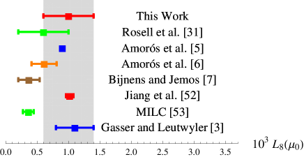
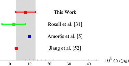
Figure 14: Comparison of the LEC predictions in this work with previous results in the bibliography.

In general, the three logarithmic OPE constraints $\alpha_{0}^{(\ell)}=\alpha_{2}^{(\ell)}=\alpha_{4}^{(\ell)}=0$ produce complex solutions for the $\lambda_{1}^{SP}$, $\lambda_{1}^{PV}$, $\lambda_{1}^{SA}$. In order to remain within the quantum field theory description, only the real values are kept. The regions with at least one real solution are shown in Fig. 15. There, we plot the allowed ranges for $c_{d}$ and $G_{V}$, with the other inputs taken at their central values. Indeed, there is no real solution for the central values $c_{d}=30$ MeV and $G_{V}=60$ MeV. On the contrary to other phenomenological analysis which seem to prefer a $c_{d}$ coupling below 30 MeV [23, 27, 28], the log OPE constraints require slightly larger values, $cd\stackrel{{\scriptstyle>}}{{{}_{\sim}}}30$ MeV. However, in general for $c_{d}$ around $30$ MeV is always impossible to have real solutions for the value of the coupling $G_{V}\simeq 64$ MeV obtained from $V$ decays [8, 9, 28]. Actually, if one demanded the $\pi\pi$ scalar form-factor (and the corresponding $\pi\pi$ contribution to the $SS$ spectral function) to vanish at high energies one would obtain $c_{d}=F^{2}/4c_{m}\simeq 42$ MeV. However, in this work we do not perform a channel by channel analysis as in Ref. [31]. Indeed, in our field theory approach one could fix separately the short-distance behaviour of the $\pi\pi$ and all the $R\pi$ channels through the $\lambda^{RR^{\prime}}$ operators, but the latter also generate $RR^{\prime}$ absorptive cuts with the wrong properties at high momentum. The only option is the global adjustment of parameters considered in this work, where the lowest channels arrange the short-distance behaviour of the highest cuts at the price of slight modifications on their couplings.

The allowed $(c_{d},G_{V})$ region of Fig. 15 actually changes if one varies the other inputs. Thus, we observed the whole range of the LECs allowed for the possible variations of the inputs and used this interval as our estimate of the central value and error. The maximum (minimum) value of the LECs was obtained at the largest (smallest) $c_{d}$ and $G_{V}$. Likewise, the most extreme LEC values were obtain when $\hat{M}_{P}$ and $M_{A}$ became smaller and $\hat{M}_{S}$ larger. These three parameters are responsible for most of the uncertainties. The impact of the $M_{V}$, $F$ and $m_{0}$ errors in the global precision is negligible.

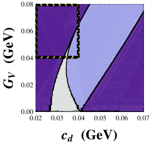
Figure 15: Allowed regions with one (light blue) or two (white) real solutions from the logarithmic OPE constraints $\alpha_{0}^{(\ell)}=\alpha_{2}^{(\ell)}=\alpha_{4}^{(\ell)}=0$. No real solution exists in the darker purple regions. In the upper left corner one can see the dashed rectangle provided by the ranges $c_{d}=30\pm 10$ MeV, $G_{V}=60\pm 20$ MeV.

The R$\chi$T computation progressively approaches the physical value as one incorporates more and more physical information. This is quite non-trivial, as the introduction of a new chiral invariant operator leads to the opening of the new absorptive cuts in addition to those channels we are in principle interested in. For instance, the $c_{m}\langle\,S\chi_{+}\,\rangle$ rules the decay into one scalar resonance and also contributes to the $S$-meson exchange in the $\pi\pi$ channel. But at the same time it also induces the decay into $S\pi$ (though other operators like $\lambda_{1}^{SP}$ are also relevant). Thus, the $\mathcal{L}_{RR^{\prime}}$ terms were used in our calculation to improve the description of the $R\pi$ channels, which were incompletely described by the linear lagrangian $\mathcal{L}_{R}$ [8]. The price to pay was that new $RR^{\prime}$ channels with two intermediate resonances showed up in our NLO computation of the correlator. Although the impact of these higher thresholds is suppressed at low energies if one chooses a convenient renormalization scheme [32, 46], their impact in the high-energy matching and OPE constraints is a priori non-trivial. In this paper we find that, indeed, the most relevant information in order to extract the low energy chiral couplings seems to be provided by the lightest cuts. On the other hand, one realizes that the values of the couplings differ from those in the full large–$N_{C}$ theory [40] and that the description of the heaviest absorptive channels may be very distorted [43]. Indeed, we obtain the resonance couplings $\lambda_{1}^{SP}=-0.22\pm 0.08$, $\lambda_{1}^{PV}=0.14\pm 0.07$ and $|\lambda_{1}^{SA}|=0.16\pm 0.14$. Even though these numbers have the right signs and order of the magnitude as the theoretical expectations $\lambda_{1}^{SP}=-\frac{d_{m}}{c_{m}}=\frac{c_{d}-2c_{m}}{2d_{m}}\sim-0.7$, $\lambda_{1}^{PV}=\frac{G_{V}}{2\sqrt{2}d_{m}}\sim 0.7$ and $\lambda_{1}^{SA}=0$ (in our analysis, for convention, we have took $c_{m}$, $d_{m}$ and $G_{V}$ as positive), their values are still far from being accurate determinations of these parameters.

8.4 Impact of the $RR^{\prime}$ channels

In this section we will make a digression on the importance of the $RR^{\prime}$ intermediate cuts that are opened after including the $\mathcal{L}_{RR^{\prime}}$ operators in the LO action. We will remove by hand the contributions with two–resonance cuts. Although this procedure is not well justified from the QFT point of view, we will perform this exercise in order make a rough comparison with the previous dispersive calculation of the octet $SS-PP$ correlator [31]. The $RR^{\prime}$ channels were neglected there, as their contribution in the dispersive integral was suppressed at low energies by inverse powers of $(M_{R}+M_{R^{\prime}})^{2}$.

Thus, we redid the calculation and removed by hand the diagrams with two–resonance cuts. This expression was then matched to the OPE at short distances, producing finally the low–energy constants,

$$L_{8}(\mu_{0})\,=\,(0.1\,\pm\,0.7)\,\cdot\,10^{-3}\,,\qquad\qquad C_{38}(\mu_{0})\,=\,(-3\,\pm\,9)\,\cdot\,10^{-6}\,,$$ (117)

where we used the same inputs as in the previous subsection. The errors are now found to be larger and, though compatible with our final result (116), the elimination of the $RR^{\prime}$ cuts decreases slightly the range for the LEC determinations, approaching them to the lower values preferred by recent ${\cal O}(p^{6})$ analysis [7] and lattice simulations [53]. However, discarding these heavier channels from the one-loop computation in this way does not seem very sound from the theoretical point of view and it is shown here just as an exercise.

9 Conclusions

In this paper, we have performed the one loop QFT calculation of the two-point $SS-PP$ correlator within R$\chi$T. We started with Ecker et al.’s lagrangian [8], containing only operators with at most one resonance field, and renormalized step by step all the relevant vertex-functions and propagators. Then we imposed OPE constraints on the full one-loop correlator, not on separate individual channels as it was performed in a previous NLO calculation [31]. Likewise, no short-distance constraint from other observables [39] was used in the present article.

After fixing part of our R$\chi$T couplings through these high-energy conditions, we expanded our result at low energies. Due to the chiral invariant structure of R$\chi$T, we were able to match the chiral logarithms and found predictions for the $\chi$PT coupling constants $L_{8}(\mu)$ and $C_{38}(\mu)$. The large discrepancy of these first numerical determinations with respect to the numbers found in the literature indicated that the simple Lagrangian $\mathcal{L}_{R}$ (with operators with at most one resonance field [8]) pointed out the need for a more complicated structure of the R$\chi$T action. The $\mathcal{L}_{R}$ terms could not fully describe the dynamics of all the two-meson intermediate channels: just the $\pi\pi$ channel description was adequately provided by the operators with at most one resonance field; all other channels ($V\pi$, $S\pi$…) did not have the right short-distance behavior. Thus, beyond any numerical discrepancy in the LECs, the absence of operators with two an three resonance fields produces a severe theoretical issue at high energies [30].

In order to arrange the $R\pi$ cuts with one resonance and one Goldstone we add all the operators $\mathcal{L}_{RR^{\prime}}$ with two resonance fields relevant for the $SS-PP$ correlator to the leading R$\chi$T lagrangian. These are the $\lambda_{1}^{SP}$, $\lambda_{1}^{PV}$ and $\lambda_{1}^{SA}$ terms given in Eq. (102). The introduction of these operators produce a dramatic improvement. When only one of them is added to the action, the LEC predictions move in the right direction, i.e., towards the range of values found in previous studies. After considering all the three $\mathcal{L}_{RR^{\prime}}$ operators, we obtain the final values for $\mu_{0}=770$ MeV,

$$L_{8}(\mu_{0})\,\,=\,\,(1.0\,\pm\,0.4)\,\cdot\,10^{-3}\,,\qquad\qquad C_{38}(\mu_{0})\,\,=\,\,(8\,\pm\,5)\,\cdot\,10^{-6}\,,$$ (118)

in reasonable agreement with the values obtained through other approaches [5, 6, 7, 31, 52, 53]. We want to remark, that this result is progressively approached as more and more complicated operators are added to the hadronic action. The terms of the lagrangian that rule the lightest channels result crucial and, thus, those determining heavier cuts not included in the analysis are expected to produce little influence.

The essential difference with the previous dispersive calculation of the $SS-PP$ correlator at NLO [31] is the presence of $RR^{\prime}$ cuts in the present work. These intermediate channels automatically show up at the very moment we place the $\mathcal{L}_{RR^{\prime}}$ operators in the R$\chi$T action. Although it is possible to demonstrate that the contribution from these heavy $RR^{\prime}$ cuts is suppressed at low energies [32, 46], their impact in high-energy conditions such as the NLO Weinber sum-rules is pretty non-trivial. The difference between the present article and Ref. [31] could be taken as a crude estimate of the impact of neglecting those higher channels.

In addition to the estimation of LECs, we also discussed some general issues about renormalization schemes within R$\chi$T. The use of the running $\widetilde{MS}$ masses $M_{R}(\mu)$ was not very convenient as their meaning changed as one added new operators to the R$\chi$T action. Thus, they were reexpressed in terms of pole masses $\hat{M}_{R}$. Likewise, we found that, with respect to the large–$N_{C}$ WSR, the NLO Weinberg sum-rules (86) led to large uncertainties and variations for the values of $c_{m}$ and $d_{m}$ derived from them in the $\widetilde{MS}$–scheme. A more convenient subtraction scheme was found to minimize these uncertainties that stemmed from the high-energy matching whereas, on the other hand, it was found to leave the low energy prediction (LABEL:eq.L8-linf) unchanged (except for the improved accuracy in the resonance coupling determination from short-distance constraints).

Appendix A Running of the renormalized parameters with $\mathcal{L}_{G}+\mathcal{L}_{R}$

When only operators with at most one resonance fields are considered in the R$\chi$T action [8], one finds before performing the meson field redefinition the running,

$$\frac{\displaystyle\partial\widetilde{L}_{8}}{\displaystyle\partial\ln\mu^{2}} = \frac{3}{512\pi^{2}F^{2}}\left[16(c_{m}^{2}-d_{m}^{2})-F^{2}-16c_{d}c_{m}+4c_{d}^{2}+2G_{V}^{2}\right]\,,$$

$$\frac{\displaystyle\partial M_{S}^{2}}{\displaystyle\partial\ln\mu^{2}} = \frac{\displaystyle\partial M_{P}^{2}}{\displaystyle\partial\ln\mu^{2}}\,=\,\frac{\displaystyle\partial c_{m}}{\displaystyle\partial\ln\mu^{2}}\,=\,\frac{\displaystyle\partial d_{m}}{\displaystyle\partial\ln\mu^{2}}\,=\,0\,,$$

$$\frac{\displaystyle\partial X_{S}}{\displaystyle\partial\ln\mu^{2}} = -\frac{3c_{d}^{2}}{16\pi^{2}F^{4}}\,,\qquad\qquad\qquad\frac{\displaystyle\partial X_{P}}{\displaystyle\partial\ln\mu^{2}}=0\,,$$

$$\frac{\displaystyle\partial\lambda^{S}_{18}}{\displaystyle\partial\ln\mu^{2}} = \frac{3c_{d}}{64\pi^{2}F^{2}}\,,\qquad\qquad\qquad\frac{\displaystyle\partial\lambda^{P}_{13}}{\displaystyle\partial\ln\mu^{2}}=0\,.$$ (119)

After the renormalization one may then consider a convenient field redefinition that removes precisely the renormalized $X_{S,P}$, $\lambda_{13}^{P}$ and $\lambda_{18}^{S}$. They (and their running) seem to disappear from the theory although their information is actually encoded in the renormalized effective couplings that remain in the action. Their running turns out to be then

$$\frac{\displaystyle\partial\widetilde{L}^{\rm eff}_{8}}{\displaystyle\partial\ln\mu^{2}} = \frac{3}{512\pi^{2}F^{2}}\left[16\,c_{m}^{2}-16\,d_{m}^{2}-F^{2}-8\,c_{d}c_{m}+2\,c_{d}^{2}+2\,G_{V}^{2}-16\,c_{d}^{2}c_{m}^{2}\right]\,,$$

$$\frac{\displaystyle\partial M_{S}^{{\rm eff}\,\,2}}{\displaystyle\partial\ln\mu^{2}} = \frac{3c_{d}^{2}M_{S}^{4}}{16\pi^{2}F^{4}}\,,\qquad\qquad\qquad\qquad\qquad\qquad\frac{\displaystyle\partial M_{P}^{{\rm eff}\,\,2}}{\displaystyle\partial\ln\mu^{2}}=0\,,$$

$$\frac{\displaystyle\partial c_{m}^{\rm eff}}{\displaystyle\partial\ln\mu^{2}} = \frac{3c_{d}M_{S}^{2}}{64\pi^{2}F^{4}}(4c_{d}c_{m}-F^{2})\,,\qquad\qquad\qquad\frac{\displaystyle\partial d_{m}^{\rm eff}}{\displaystyle\partial\ln\mu^{2}}=0\,.$$ (120)

Appendix B On-shell scheme for $c_{m}$ and $d_{m}$

This would be a continuation of the pole-mass scheme. In addition to this, the renormalized on-shell couplings $\hat{c}_{m}$ and $\hat{d}_{m}$ are prescribed, respectively, by the real part of the residue of the correlator at the scalar and the pseudoscalar resonance poles [31, 32]. This was the scheme considered in the dispersive approach from Refs. [31, 32]. The shift $\Delta\kappa$ with respect to the $\widetilde{MS}$–subtraction prescription is given up to NLO in $1/N_{C}$ by

$$2\,c_{m}\Delta c_{m} = c_{m}^{2}-\hat{c}_{m}^{2}\,=\,\frac{\displaystyle c_{m}}{\displaystyle 2B_{0}}\,\mbox{Re}\Phi_{sS}^{r}(M_{S}^{2})^{1\ell}\,\,-\,\,c_{m}^{2}\,\mbox{Re}\Sigma_{S}^{r\,\,^{\prime}}(M_{S}^{2})^{1\ell}\,,$$

$$2\,d_{m}\Delta d_{m} = d_{m}^{2}-\hat{d}_{m}^{2}\,=\,\frac{\displaystyle d_{m}}{\displaystyle 2B_{0}}\,\mbox{Re}\Phi_{pP}^{r}(M_{P}^{2})^{1\ell}\,\,-\,\,d_{m}^{2}\,\mbox{Re}\Sigma_{P}^{r\,\,^{\prime}}(M_{P}^{2})^{1\ell}\,.$$ (121)

In the case where only $\mathcal{L}_{R}$ interactions are considered, one has

$$2\,c_{m}\Delta c_{m} = \frac{\displaystyle 4\,c_{d}c_{m}}{\displaystyle F^{2}}\,\frac{\displaystyle 3\,M_{S}^{2}}{\displaystyle 128\pi^{2}}\left[-1+\left(1-\frac{\displaystyle 4\,c_{d}c_{m}}{\displaystyle F^{2}}\right)\ln\frac{\displaystyle M_{S}^{2}}{\displaystyle\mu^{2}}\right]\,,$$

$$2\,d_{m}\Delta d_{m} = 0\,.$$ (122)

Appendix C Feynman integrals

The scalar integrals are

$$A_{0}(M^{2}) = \int\frac{dk^{d}}{i(2\pi)^{d}}\frac{1}{k^{2}-M^{2}+i\epsilon},$$

$$B_{0}(p^{2},M_{a}^{2},M_{b}^{2}) = \int\frac{dk^{d}}{i(2\pi)^{d}}\frac{1}{(k^{2}-M_{a}^{2}+i\epsilon)[(p-k)^{2}-M_{b}^{2}+i\epsilon]}$$ (123)

Using the formula in [30] we use the following expansions

$$A_{0}(M^{2}) = \frac{-M^{2}}{16\pi^{2}}\Bigg{\{}\lambda_{\infty}+\ln\frac{M^{2}}{\mu^{2}}\Bigg{\}},$$

$$B_{0}(p^{2},0,0) = -\frac{1}{16\pi^{2}}\Bigg{\{}\lambda_{\infty}-1+\ln\left(\frac{-p^{2}}{\mu^{2}}\right)\Bigg{\}},$$

$$B_{0}(p^{2},0,M^{2}) = -\frac{1}{16\pi^{2}}\Bigg{\{}\lambda_{\infty}+\ln\frac{M^{2}}{\mu^{2}}-1+\left(1-\frac{M^{2}}{p^{2}}\right)\ln\left(1-\frac{p^{2}}{M^{2}}\right)\Bigg{\}},$$

$$B_{0}(p^{2},M^{2},M^{2}) = -\frac{1}{16\pi^{2}}\Bigg{\{}\lambda_{\infty}+\ln\frac{M^{2}}{\mu^{2}}-1+\sigma_{M}\ln\left(\frac{\sigma_{M}+1}{\sigma_{M}-1}\right)\Bigg{\}}$$ (124)

$$\overline{J}(p^{2},M_{a}^{2},M_{b}^{2}) = \frac{1}{32\pi^{2}}\left\{2+\left[\frac{\displaystyle M_{a}^{2}-M_{b}^{2}}{\displaystyle p^{2}}\,-\,\frac{\displaystyle M_{a}^{2}+M_{b}^{2}}{\displaystyle M_{a}^{2}-M_{b}^{2}}\right]\ln\frac{\displaystyle M_{b}^{2}}{\displaystyle M_{a}^{2}}\right.$$

$$\left.\,-\,\frac{\displaystyle\lambda^{1/2}(p^{2},M_{a}^{2},M_{b}^{2})}{\displaystyle p^{2}}\,\ln\left(\frac{\displaystyle\left[p^{2}+\lambda^{1/2}(p^{2},M_{a}^{2},M_{b}^{2})\right]^{2}-(M_{a}^{2}-M_{b}^{2})^{2}}{\displaystyle\left[p^{2}-\lambda^{1/2}(p^{2},M_{a}^{2},M_{b}^{2})\right]^{2}-(M_{a}^{2}-M_{b}^{2})^{2}}\right)\right\}\,,$$

where $\sigma_{M}=\sqrt{1-4M^{2}/p^{2}}$ and $\lambda(x,y,z)=(x-y-z)^{2}-4yz$.

Appendix D Useful expansions

Using expansions for $x\rightarrow\infty$

$$\phi(x) = \ln(-x)-1-\frac{3\ln(-x)}{x}+\frac{3}{2x}+\frac{3\ln(-x)}{x^{2}}+\frac{3}{2x^{2}}+\dots,$$

$$\psi(x) = -\ln(-x)+\frac{2\ln(-x)}{x}-\frac{\ln(-x)}{x^{2}}-\frac{3}{2x^{2}}+\dots,$$

$$(1-\frac{1}{x})\ln(1-x) = \ln(-x)-\frac{\ln(-x)}{x}-\frac{1}{x}+\frac{1}{2x^{2}}+\dots$$

References

• [1] S. Weinberg, Physica A 96 (1979) 327.
• [2] J. Gasser and H. Leutwyler, Annals Phys. 158 (1984) 142.
• [3] J. Gasser and H. Leutwyler, Nucl. Phys. B 250 (1985) 465.
• [4] J. Bijnens, G. Colangelo and G. Ecker, Annals Phys. 280 (2000) 100-139 [arXiv:hep-ph/9907333]; JHEP 9902 (1999) 020 [arXiv:hep-ph/9902437].
• [5] G. Amorós, J. Bijnens and P. Talavera, Nucl. Phys. B 568 (2000) 319-363 [arXiv:hep-ph/9907264].
• [6] G. Amorós, J. Bijnens and P. Talavera, Nucl. Phys. B 602 (2001) 87 [arXiv:hep-ph/0101127].
• [7] J. Bijnens and I. Jemos, [arXiv:0909.4477 [hep-ph]].
• [8] G. Ecker, J. Gasser, A. Pich and E. de Rafael, Nucl. Phys. B 321 (1989) 311.
• [9] G. Ecker, J. Gasser, H. Leutwyler, A. Pich and E. de Rafael, Phys. Lett. B 223 (1989) 425.
• [10] G. ’t Hooft, Nucl. Phys.  B 72 (1974) 461; 75 (1974) 461; E. Witten, Nucl. Phys.  B 160 (1979) 57.
• [11] K. Kampf, J. Novotny and J. Trnka, Eur. Phys. J.  C 50 (2007) 385 [arXiv:hep-ph/0608051].
• [12] K. Kampf, J. Novotný and J. Trnka, Acta Phys. Polon. B 38 (2007) 2961-2966 [arXiv:hep-ph/0701041].
• [13] J. Bijnens and E. Pallante, Mod. Phys. Lett. A 11 (1996) 1069-1080 [arXiv:hep-ph/9510338].
• [14] P. D. Ruiz-Femenia, A. Pich and J. Portoles, JHEP 0307 (2003) 003 [arXiv:hep-ph/0306157].
• [15] V. Cirigliano, G. Ecker, M. Eidemuller, R. Kaiser, A. Pich and J. Portolés, Nucl. Phys. B 753 (2006) 139-177 [arXiv:hep-ph/0603205].
• [16] V. Cirigliano, G. Ecker, M. Eidemüller, R. Kaiser, A. Pich and J. Portolés, JHEP 0504 (2005) 006 [arXiv:hep-ph/0503108].
• [17] V. Cirigliano, G. Ecker, M. Eidemuller, J. Portoles and A. Pich, Phys. Lett. B 596 (2004) 96 [arXiv:hep-ph/0404004].
• [18] B. Moussallam, Phys. Rev. D 51 (1995) 4939-4949 [arXiv:hep-ph/9407402]; Nucl. Phys. B 504 (1997) 381 [arXiv:hep-ph/9701400]; JHEP bf 0008 (2000) 005 [arXiv:hep-ph/0005245]; B. Ananthanarayan and B. Moussallam, JHEP 0406 (2004) 047 [arXiv:hep-ph/0405206].
• [19] J. Bijnens, E. Gamiz, E. Lipartia and J. Prades, JHEP 0304 (2003) 055 [arXiv:hep-ph/0304222].
• [20] M. Knecht and A. Nyffeler, Eur. Phys. J. C 21 (2001) 659-678 [arXiv:hep-ph/0106034].
• [21] K. Kampf and B. Moussallam, Eur. Phys. J. C 47 (2006) 723-736 [arXiv:hep-ph/0604125].
• [22] P. Roig, [arXiv:0709.3734 [hep-ph]]; D. Gómez-Dumm, P. Roig, A. Pich and J. Portolés, [arXiv:0911.2640 [hep-ph]].
• [23] S. Ivashyn and A.Yu. Korchin, Eur. Phys. J. C 54 (2008) 89-106 [arXiv:0707.2700 [hep-ph]].
• [24] S. Ivashyn and A.Yu. Korchin, [arXiv:0904.4823 [hep-ph]].
• [25] Z. H. Guo, J. J. Sanz-Cillero and H. Q. Zheng, Phys. Lett.  B 661 (2008) 342-347 [arXiv:0710.2163 [hep-ph]].
• [26] M. Jamin, J.A. Oller and A. Pich, Nucl. Phys. B bf 587 (2000) 331-362 [arXiv:hep-ph/0006045].
• [27] Pere Masjuan, [arXiv:0910.0140 [hep-ph]].
• [28] Z.-H. Guo and J.J. Sanz-Cillero, Phys. Rev. D 79 (2009) 096006 [arXiv:0903.0782 [hep-ph]].
• [29] O. Cata and S. Peris, Phys. Rev. D 65 (2002) 056014 [arXiv:hep-ph/0107062].
• [30] I. Rosell, J. J. Sanz-Cillero and A. Pich, JHEP 0408 (2004) 042 [arXiv:hep-ph/0407240].
• [31] I. Rosell, J. J. Sanz-Cillero and A. Pich, JHEP 0701 (2007) 039 [arXiv:hep-ph/0610290].
• [32] A. Pich, I. Rosell and J. J. Sanz-Cillero, JHEP 0807 (2008) 042 [arXiv:0803.1567 [hep-ph]].
• [33] I. Rosell, P. Ruiz-Femenía and J. Portolés, JHEP 0512 (2005) 020 [arXiv:hep-ph/0510041].
• [34] J.J. Sanz-Cillero, Phys. Lett. B 649 (2007) 180-185 [arXiv:hep-ph/0702217].
• [35] L.Y. Xiao and J.J. Sanz-Cillero, Phys. Lett. B 659 (2008) 452-456 [arXiv:0705.3899 [hep-ph]]; J. J. Sanz-Cillero [arXiv:0709.3363].
• [36] K. Kampf, J. Novotny and J. Trnka, Fizika B 17 (2008) 2, 349 - 354 [arXiv:0803.1731 [hep-ph]].
• [37] K. Kampf, J. Novotny and J. Trnka, Nucl. Phys. Proc. Suppl. 186 (2009) 153-156 [arXiv:0810.3842 [hep-ph]].
• [38] J.J. Sanz-Cillero, Phys. Lett. B 681 (2009) 100-104 [arXiv:0905.3676 [hep-ph]].
• [39] A. Pich, [arXiv:0812.2631 [hep-ph]], and references therein.
• [40] M. Golterman and S. Peris, Phys. Rev. D 74 (2006) 096002 [arXiv:hep-ph/0607152].
• [41] M.A. Shifman, A.I. Vainshtein and V.I. Zakharov, Nucl. Phys. B 147 (1979) 385-447; 147 (1979) 448-518.
• [42] S. Weinberg, Phys. Rev. Lett.  18 (1967) 507.
• [43] P. Masjuan and S. Peris, JHEP 0705 (2007) 040 [arXiv:0704.1247 [hep-ph]].
• [44] M. Knecht and E. de Rafael, Phys. Lett. B 424 (1998) 335-342 [arXiv:hep-ph/9712457]; S. Peris, M. Perrottet and E. de Rafael, JHEP 9805 (1998) 011 [arXiv:hep-ph/9805442].
• [45] K. Kampf, J. Novotny and J. Trnka, Fizika B 17 (2008) 349; Nucl. Phys. Proc. Suppl.  186 (2009) 153; arXiv:0905.1348 [hep-ph]; in preparation.
• [46] I. Rosell, Ph.D.Thesis (U. Valencia, 2007) [arXiv:hep-ph/0701248];
• [47] I. Rosell, P. Ruiz-Femenía and J.J. Sanz-Cillero, Phys. Rev. D 79 (2009) 076009 [arXiv:0903.2440 [hep-ph]]; J. Portolés, I. Rosell and Pedro Ruiz-Femenia, Phys. Rev. D 75 (2007) 114011 [arXiv:hep-ph/0611375].
• [48] J.J. Sanz-Cillero, Ph.D. Thesis (U. Valencia, 2004).
• [49] M. F. L. Golterman and S. Peris, Phys. Rev.  D 61 (2000) 034018 [arXiv:hep-ph/9908252].
• [50] H. Leutwyler, Nucl. Phys. Proc. Suppl. 64 (1998) 223-231 [arXiv:hep-ph/9709408]; R. Kaiser and H. Leutwyler, Eur. Phys. J. C 17 (2000) 623-649 [arXiv:hep-ph/0007101]; [arXiv:hep-ph/9806336].
• [51] C. Amsler et al. (Particle Data Group), Phys. Lett. B 667 (2008) 1 (2008) and 2009 partial update for the 2010 edition, http://pdglive.lbl.gov .
• [52] S.-Z. Jiang, Y. Zhang, C. Li and Q. Wang, [arXiv:0907.5229 [hep-ph]].
• [53] A. Bazavov et al. (MILC Collaboration), [arXiv:0910.3618 [hep-lat]].