Validity of the factorization approximation and correlation induced by nonextensivity in $N$-unit independent systems

Abstract

We have discussed the validity of the factorization approximation (FA) and nonextensivity-induced correlation, by using the multivariate $q$-Gaussian probability distribution function (PDF) for $N$-unit identical, independent nonextensive systems. The Tsallis entropy is shown to be expressed by $S_{q}^{(N)}=S_{q,FA}^{(N)}+\Delta S_{q}^{(N)}$ where $q$ denotes the entropic index, $S_{q,FA}^{(N)}$ a contribution in the FA, and $\Delta S_{q}^{(N)}$ a correction term. It is pointed out that the correction term of $\Delta S_{q}^{(N)}$ is considerable for large $|q-1|$ and/or large $N$ because the multivariate PDF cannot be expressed by the factorized form which is assumed in the FA. This implies that the pseudoadditivity of the Tsallis entropy, which is obtained with PDFs in the FA, does not hold although it is commonly postulated in the literatures. We have calculated correlations defined by $C_{m}=\langle(\delta x_{i}\>\delta x_{j})^{m}\rangle_{q}-\langle(\delta x_{i})^{m}\rangle_{q}\>\langle(\delta x_{j})^{m}\rangle_{q}$ for $i\neq j$, where $\delta x_{i}=x_{i}-\langle x_{i}\rangle_{q}$ and $\langle\cdot\rangle_{q}$ stands for $q$-average over the escort PDF. It has been shown that $C_{1}$ expresses the intrinsic correlation and that $C_{m}$ with $m\geq 2$ signifies correlation induced by nonextensivity whose physical origin is elucidated within the superstatistics. PDFs calculated for the classical ideal gas and harmonic oscillator are compared with the $q$-Gaussian PDF. A discussion on the $q$-product PDF is presented also.

I Introduction

In the last decade, much attention has been paid to the nonextensive statistics since Tsallis proposed the so-called Tsallis entropy Tsallis88 ; Tsallis98 ; Tsallis01 ; Tsallis04 . The Tsallis entropy for $N$-unit nonextensive systems is defined by

$$S_{q}^{(N)} = \frac{k_{B}}{q-1}\left(1-\int\left[p_{q}^{(N)}(\mbox{\boldmath$x$})\right]^{q}\>d\mbox{\boldmath$x$}\right),$$ (1)

where $q$ is the entropic index, $k_{B}$ the Boltzmann constant ($k_{B}=1$ hereafter), $p_{q}^{(N)}(\mbox{\boldmath$x$})$ denotes the $N$-variate probability distribution function (PDF), $\mbox{\boldmath$x$}=\{x_{i}\}$ ($i=1$ to $N$), and $d\mbox{\boldmath$x$}=\prod_{i=1}^{N}dx_{i}$. The Tsallis entropy is a one-parameter generalization of the Boltzmann-Gibbs entropy, to which the Tsallis entropy reduces in the limit of $q\rightarrow 1.0$. The Tsallis entropy is nonextensive (non-additive), which is shown in the literatures as follows Tsallis88 ; Tsallis98 ; Tsallis01 ; Tsallis04 . When the PDF for two independent subsystems $A$ and $B$ is factorized into those of $A$ and $B$ ($x_{1}\in A,\;x_{2}\in B$),

$$p_{q}^{(2)}(x_{1},x_{2}) = p_{q}^{(1)}(x_{1})\>p_{q}^{(1)}(x_{2}),$$ (2)

Eq. (1) yields

$$S_{q}^{(2)}(A+B) = S_{q}^{(1)}(A)+S_{q}^{(1)}(B)+(1-q)S_{q}^{(1)}(A)\>S_{q}^{(1)}(B),$$ (3)

which is referred to as the $pseudoadditive$ relation. When the PDF for $N$-unit independent subsystems is given as factorized form,

$$p_{q}^{(N)}(\mbox{\boldmath$x$}) = \prod_{i=1}^{N}\>p_{q}^{(1)}(x_{i}),$$ (4)

we obtain the pseudoadditive Tsallis entropy $S_{q}^{(N)}$ which is expressed by

$$\ln\left[1+(1-q)S_{q}^{(N)}\right] = \sum_{i=1}^{N}\ln\left[1+(1-q)S_{q}^{(1)}(i)\right].$$ (5)

It should be, however, noted that Eqs. (3) and (5) are not correct in the strict sense because the bivariate PDF derived by the maximum-entropy method (MEM) cannot be expressed by Eq. (2) or (4), as will be shown shortly [Eq. (37)]. Indeed, our calculation for identical, independent systems with the use of exact multivariate PDFs to Eq. (1) yields

$$S_{q}^{(2)} = 2S_{q}^{(1)}+(1-q)\left[S_{q}^{(1)}\right]^{2}+\Delta S_{q}^{(2)},$$ (6)

$$S_{q}^{(N)} = S_{q,FA}^{(N)}+\Delta S_{q}^{(N)},$$ (7)

where $S_{q,FA}^{(N)}$ denotes $S_{q}^{(N)}$ in Eq. (5) evaluated by the PDF of Eq. (4) in the factorized approximation (FA), and $\Delta S_{q}^{(N)}$ expresses a correction term [Eq. (44)]. Equations (6) and (7) show that $S_{q}^{(N)}$ does not satisfy the pseudoadditivity.

The PDF is evaluated by the MEM for the Tsallis entropy with imposing some constraints. At the moment, there are four possible MEMs: (a) original method Tsallis88 , (b) un-normalized method Curado91 , (c) normalized method Tsallis98 , and (d) the optimal Lagrange multiplier (OLM) method Martinez00 . A comparison among the four MEMs is made in Ref. Tsallis04 . Although the four methods are equivalent in the sense that PDFs derived in them are easily transformed to each other Ferri05 , obtained expressions for physical quantities are ostensibly different depending on the adopted MEM.

Let us consider $N$-unit independent systems whose hamiltonian is given by

$$H = \sum_{i=1}^{N}\>h_{i}.$$ (8)

PDFs for the hamiltonian in the Boltzmann-Gibbs statistics ($q=1.0$) may be calculated with the use of either $H$ or $h_{i}$ because they are given by

$$p_{1}^{(N)}(\mbox{\boldmath$x$}) \propto {\rm Tr}\;e^{-\beta H}=\prod_{i=1}^{N}\;p_{1}^{(1)}(x_{i}),$$ (9)

$$p_{1}^{(1)}(x_{i}) \propto {\rm Tr}_{i}\;e^{\beta h_{i}},$$ (10)

where $\beta$ is the inverse of temperature, Tr denotes the full trace and ${\rm Tr}_{i}$ the partial trace over $i$. It is, however, not the case in the nonextensive statistics in which PDFs are given by

$$p_{q}^{(N)}(\mbox{\boldmath$x$}) \propto {\rm Tr}\;\exp_{q}\left(-\beta H\right),$$ (11)

$$\neq \prod_{i=1}^{N}\;p_{q}^{(1)}(x_{i})\hskip 56.9055pt\mbox{for $q\neq 1.0$},$$ (12)

$$p_{q}^{(1)}(x_{i}) \propto {\rm Tr}_{i}\;\exp_{q}(-\beta h_{i}).$$ (13)

Here $\exp_{q}(x)$ expresses the $q$-exponential function defined by

$$\exp_{q}(x) = [1+(1-q)x]_{+}^{1/(1-q)},$$ (14)

with $[x]_{+}={\rm max}(x,0)$, which reduces to $\exp_{q}(x)=e^{x}$ for $q\rightarrow 1.0$. The inequality in Eq. (12) arises from the properties of the $q$-exponential function,

$$\exp_{q}(x+y) \neq \exp_{q}(x)\exp_{q}(y)\hskip 56.9055pt\mbox{for $q\neq 1.0$}.$$ (15)

Then it has been controversial whether we should employ $H$ or $h_{i}$ in calculating the PDF in the nonextensive statistics. In many applications of the nonextensive statistics, one usually calculates $p_{1}(x_{i})$ with the use of $h_{i}$ in Eq. (13), explicitly or implicitly employing the FA, because an exact evaluation of $p_{N}(\mbox{\boldmath$x$})$ in Eq. (11) is generally difficult. This issue of the degree of freedom $N$ on the PDF has been discussed in Refs. Wang02 ; Wang02b ; Jiulin09 . A calculation for $N$-unit harmonic oscillator shows that the partition function obtained in the FA is quite different from that obtained by the exact PDF Lenzi01 , related discussion being given in Sec. IIIC.

In our previous papers Hasegawa08b ; Hasegawa09 , we discussed the effect of spatial correlation on the Tsallis entropy and the generalized Fisher information in nonextensive systems. We obtained the multivariate $q$-Gaussian PDF with the OLM-MEM Martinez00 , which correctly includes correlation. It is the purpose of the present paper to discuss the issue mentioned above, by using the exact multivariate $q$-Gaussian PDF derived in Ref. Hasegawa08b . One of the advantages of a use of the $q$-Gaussian PDF is that it is free from an ambiguity in defining the physical temperature in conformity with the zeroth law of thermodynamics in the nonextensive statistics Tsallis04 . From calculations of the Tsallis entropy and correlation in $N$-unit independent systems, we will show the importance of effects which are not taken into account in the FA. The nonextensivity-induced correlation has been discussed for classical ideal gas Abe99b ; Liyan08 ; Feng10 and harmonic oscillator Liyan08 .

The superstatistics is one of alternative approaches to the nonextensive statistics besides the MEM Wilk00 ; Beck01 ; Beck05 (for a recent review, see Beck07 ). In the superstatistics, it is assumed that locally the equilibrium state of a given system is described by the Boltzmann-Gibbs statistics and its global properties may be expressed by a superposition over the fluctuating intensive parameter (i.e., the inverse temperature) Wilk00 -Beck07 . The superstatistics has been adopted in many kinds of subjects such as hydrodynamic turbulence, cosmic ray and solar flares Beck07 . The physical origin of the nonextensivity-induced correlation may be elucidated within the superstatistics.

The paper is organized as follows. In Sec. II, multivariate PDFs for correlated nonextensive systems derived by the OLM-MEM Martinez00 are briefly discussed Hasegawa08b ; Hasegawa09 . By using the multivariate PDF, we calculate the Tsallis entropy and correlations. Some model calculations of the $q$- and $N$-dependent Tsallis entropy and correlations are presented. In Sec. III, we discuss the physical origin of the nonextensivity-induced correlation, calculating the PDF within the superstatistics Wilk00 ; Beck01 . PDFs of the one-dimensional classical ideal gas and harmonic oscillators derived with the use of the OLM-MEM Martinez00 are compared with the $q$-Gaussian PDF. The PDF expressed by the $q$-product Borges04 is also discussed. Sec. IV is devoted to our conclusion.

II $q$-Gaussian PDF

II.1 OLM-MEM

We consider $N$-unit nonextensive systems whose PDF, $p_{q}^{(N)}(\mbox{\boldmath$x$})$, is derived with the use of the OLM-MEM Martinez00 for the Tsallis entropy given by Eq. (1) Tsallis88 ; Tsallis98 . We impose four constraints given by (for details, see Appendix B of Ref. Hasegawa08b )

$$1 = \int p_{q}^{(N)}(\mbox{\boldmath$x$})\>d\mbox{\boldmath$x$},$$ (16)

$$\mu = \frac{1}{N}\sum_{i=1}^{N}\langle x_{i}\rangle_{q},$$ (17)

$$\sigma^{2} = \frac{1}{N}\sum_{i=1}^{N}\langle(x_{i}-\mu)^{2}\rangle_{q},$$ (18)

$$s\>\sigma^{2} = \frac{1}{N(N-1)}\sum_{i=1}^{N}\sum_{j=1(\neq i)}^{N}\langle(x_{i}-\mu)(x_{j}-\mu)\rangle_{q}.$$ (19)

Here $\mu$, $\sigma^{2}$ and $s$ express the mean, variance, and degree of intrinsic correlation, respectively, and $\langle\cdot\rangle_{q}$ denotes the $q$-average over the escort PDF,

$$P_{q}^{(N)}(\mbox{\boldmath$x$}) = \frac{\left[p_{q}^{(N)}(\mbox{\boldmath$x$})\right]^{q}}{c_{q}^{(N)}},$$ (20)

with

$$c_{q}^{(N)} = \int\left[p_{q}^{(N)}(\mbox{\boldmath$x$})\right]^{q}\>d\mbox{\boldmath$x$}.$$ (21)

Evaluations of the $q$-average with the use of the exact approach Prato95 ; Rajagopal98 are discussed in Appendix A.

The OLM-MEM with the constraints given by Eqs. (16)-(19) leads to the PDF given by Hasegawa08b

$$p_{q}^{(N)}(\mbox{\boldmath$x$}) = \frac{1}{Z_{q}^{(N)}}\exp_{q}\left[-\left(\frac{1}{2\nu_{q}^{(N)}\sigma^{2}}\right)\Phi(\mbox{\boldmath$x$})\right],$$ (22)

where

$$\Phi(\mbox{\boldmath$x$}) = \sum_{i=1}^{N}\sum_{j=1}^{N}[a_{0}\>\delta_{ij}+a_{1}(1-\delta_{ij})](x_{i}-\mu)(x_{j}-\mu),$$ (23)

$$a_{0} = \frac{[1+(N-2)s]}{(1-s)[1+(N-1)s]},$$ (24)

$$a_{1} = -\frac{s}{(1-s)[1+(N-1)s]},$$ (25)

$$Z_{q}^{(N)}=\left\{\begin{array}[]{ll}r_{s}^{(N)}\left[\frac{2\pi\nu_{q}^{(N)}\sigma^{2}}{q-1}\right]^{N/2}\frac{\Gamma\left(\frac{1}{q-1}-\frac{N}{2}\right)}{\Gamma\left(\frac{1}{q-1}\right)}&\mbox{for $q>1$},\\ r_{s}^{(N)}(2\pi\sigma^{2})^{N/2}&\mbox{for $q=1$},\\ r_{s}^{(N)}\left[\frac{2\pi\nu_{q}^{(N)}\sigma^{2}}{1-q}\right]^{N/2}\frac{\Gamma\left(\frac{1}{1-q}+1\right)}{\Gamma\left(\frac{1}{1-q}+1+\frac{N}{2}\right)}&\mbox{for $q<1$},\end{array}\right.$$ (29)

$$r_{s}^{(N)} = \{(1-s)^{N-1}[1+(N-1)s]\}^{1/2},$$ (30)

$$\nu_{q}^{(N)} = \frac{(N+2)-Nq}{2},$$ (31)

$B(x,y)$ and $\Gamma(z)$ denoting the beta and gamma functions, respectively. Hereafter we assume that the entropic index $q$ takes a value,

$$0<q<1+\frac{2}{N},$$ (32)

because $p_{q}^{(N)}(\mbox{\boldmath$x$})$ given by Eq. (22) has the probability properties with $\nu_{q}^{(N)}>0$ for $q<1+2/N$ and because the Tsallis entropy is stable for $q>0$ Abe02 .

In the absence of the intrinsic correlation ($s=0$) for which

$$\Phi(\mbox{\boldmath$x$}) = \sum_{i}\>(x_{i}-\mu)^{2},$$ (33)

Eq. (22) reduces to

$$p_{q}^{(N)}(\mbox{\boldmath$x$}) = \frac{1}{Z_{q}^{(N)}}\exp_{q}\left[-\left(\frac{1}{2\nu_{q}^{(N)}\sigma^{2}}\right)\sum_{i=1}^{N}\>(x_{i}-\mu)^{2}\right].$$ (34)

On the other hand, the PDF in the FA is given by

$$p_{q,FA}^{(N)}(\mbox{\boldmath$x$}) = \prod_{i=1}^{N}\>p_{q}^{(1)}(x_{i}),$$ (35)

$$= \frac{1}{\left(Z_{q}^{(1)}\right)^{N}}\prod_{i=1}^{N}\exp_{q}\left[-\left(\frac{1}{2\nu_{q}^{(1)}\sigma^{2}}\right)\>(x_{i}-\mu)^{2}\right].$$ (36)

In Eqs. (34) and (36), $Z_{q}^{(N)}$ is given by Eq. (29) with $r_{s}^{(N)}=1.0$. From a comparison between Eqs. (34) and (36), it is evident that

$$p_{q}^{(N)}(\mbox{\boldmath$x$}) \neq p_{q,FA}^{(N)}(\mbox{\boldmath$x$}),$$ (37)

except for $q=1.0$ or $N=1$.

II.2 Tsallis entropy

Substituting the PDF given by Eqs. (22)-(31) to Eq. (1), we first calculate the Tsallis entropy which is given by Hasegawa08b

$$S_{q}^{(N)} = \frac{1-c_{q}^{(N)}}{q-1},$$ (38)

with

$$c_{q}^{(N)} = \nu_{q}^{(N)}\left[Z_{q}^{(N)}\right]^{1-q}.$$ (39)

The $s$-dependence of the Tsallis entropy was previously discussed (see Fig. 1 of Ref. Hasegawa08b ). With increasing $s$, the Tsallis entropy is decreased as given by

$$S_{q}^{(N)}(s) = S_{q}^{(N)}(0)-\frac{N(N-1)c_{q}^{(N)}}{4}\>s^{2}\hskip 28.45274pt\mbox{for $|s|\ll 2/\sqrt{N(N-1)}$ }.$$ (40)

Now we pay our attention to identical, independent systems with $s=0$, for which we obtain

$$S_{q}^{(N)} = S_{q,FA}^{(N)}+\Delta S_{q}^{(N)},$$ (41)

with

$$S_{q,FA}^{(N)} = \frac{1-(c_{q}^{(1)})^{N}}{q-1},$$ (42)

$$\Delta S_{q}^{(N)} = \left(\frac{1}{q-1}\right)[(c_{q}^{(1)})^{N}-c_{q}^{(N)}],$$ (43)

$$= \left(\frac{1}{q-1}\right)\left(\left[\nu_{q}^{(1)}(Z_{q}^{(1)})^{1-q}\right]^{N}-\nu_{q}^{(N)}(Z_{q}^{(N)})^{1-q}\right).$$ (44)

Here $S_{q,FA}^{(N)}$ denotes the Tsallis entropy calculated in the FA, and $\Delta S_{q}^{(N)}$ signifies a correction term. Equation (5) leads to

$$S_{q,FA}^{(N)} = \sum_{k=1}^{N}\frac{N!}{(N-k)!\>k!}(1-q)^{k-1}(S_{q}^{(1)})^{k},$$ (45)

$$= NS_{q}^{(1)}+\frac{N(N-1)(1-q)}{2}(S_{q}^{(1)})^{2}+\cdot\cdot.$$ (46)

In particular for $N=2$, Eq. (41) becomes

$$S_{q}^{(2)} = \frac{1-c_{q}^{(2)}}{q-1}=S_{q,FA}^{(2)}+\Delta S_{q}^{(2)},$$ (47)

with

$$S_{q,FA}^{(2)} = \frac{1-(c_{q}^{(1)})^{2}}{q-1}=2S_{q}^{(1)}+(1-q)(S_{q}^{(1)})^{2},$$ (48)

$$\Delta S_{q}^{(2)} = \left(\frac{1}{q-1}\right)[(c_{q}^{(1)})^{2}-c_{q}^{(2)}],$$ (49)

$$= \left(\frac{1}{q-1}\right)\left(\left[\nu_{q}^{(1)}(Z_{q}^{(1)})^{1-q}\right]^{2}-\nu_{q}^{(2)}(Z_{q}^{(2)})^{1-q}\right).$$ (50)

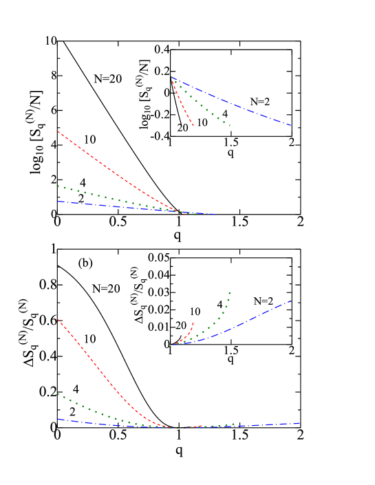
Figure 1: (Color online) The $q$ dependence of (a) $S_{q}^{(N)}/N$ and (b) $\Delta S_{q}^{(N)}/S_{q}^{(N)}$ for $N=2$ (chain curves), 4 (dotted curves), 10 (dashed curves) and 20 (solid curves): insets show enlarged plots for $q\geq 1.0$: the ordinates in (a) are in the logarithmic scale.

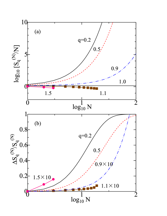
Figure 2: (Color online) (a) $\log_{10}[S_{q}^{(N)}/N]$ and (b) $\Delta S_{q}^{(N)}/S_{q}^{(N)}$ as a function of $\log_{10}N$ for $q=0.2$ (solid curves), 0.5 (dashed curves), 0.9 (chain curves), 1.1 (squares) and 1.5 (circles): results for $q=0.9$, 1.1 and 1.5 in (b) are multiplied by a factor of ten. Note that, for $q=1.0$, $S_{q}^{(N)}/N=1.4189$ and $\Delta S_{q}^{(N)}/S_{q}^{(N)}=0$ independently of $N$.

We will show some model calculations of $S_{q}^{(N)}$ and $\Delta S_{q}^{(N)}$. The $q$ dependences of $\log_{10}(S_{q}^{(N)}/N)$ for various $N$ values are shown in Fig. 1(a) where the inset shows an enlarged plot for $q\geq 1.0$. With decreasing $q$ from unity, $S_{q}^{(N)}$ is logarithmically increased. The $N$ dependence of $\Delta S_{q}^{(N)}/S_{q}^{(N)}$ is shown in Fig. 1(b) where the inset again shows an enlarged plot for $q\geq 1.0$. We note that $\Delta S_{q}^{(2)}/S_{q}^{(2)}$ is 0.049, 0.0 and 0.025 for $q=0.0$, 1.0 and 2.0, respectively. When $N$ is more increased, $\Delta S_{q}^{(N)}/S_{q}^{(N)}$ becomes more considerable. For example, its value becomes 0.61 and 0.91 for $N=10$ and 20, respectively, at $q=0.0$.

The $N$ dependence of $\log_{10}(S_{q}^{(N)}/N)$ is shown in Fig. 2(a). We note that with increasing $N$, $S_{q}^{(N)}$ is increased (decreased) for $q<1.0$ ($q>1.0$). The $N$ dependence of $\Delta S_{q}^{(N)}/S_{q}^{(N)}$ is shown in Fig. 2(b) where results for $q=0.9$, 1.1 and 1.5 are multiplied by a factor of ten. It is realized that for $q=0.2$ and 0.5, $\Delta S_{q}^{(N)}/S_{q}^{(N)}\rightarrow 1.0$ as $N\rightarrow 100$ where $S_{q,FA}^{(N)}$ almost completely underestimates the Tsallis entropy.

Figures 1(b) and 2(b) clearly show that $\Delta S_{q}^{(N)}/S_{q}^{(N)}$ is positive and becomes appreciable for large values of $N$ and/or large $|q-1|$, in particular for $q<1$.

II.3 Correlation

Next we calculate correlations for $i\neq j$ defined by

$$C_{m} \equiv \langle(\delta x_{i}\>\delta x_{j})^{m}\rangle_{q}-\langle(\delta x_{i})^{m}\rangle_{q}\>\langle(\delta x_{i})^{m}\rangle_{q},$$ (51)

where $\delta x_{i}=x_{i}-\mu$. With the use of the PDF given by Eqs. (22)-(31), we obtain the first- and second-order correlations given by (for details, see Appendix A)

$$C_{1} = \sigma^{2}s,$$ (52)

$$C_{2} = C_{2s}+C_{2n},$$ (53)

where

$$C_{2s} = \frac{2[(N+2)-Nq]\>\sigma^{4}s^{2}}{[(N+4)-(N+2)q]},$$ (54)

$$= \left\{\begin{array}[]{ll}0&\mbox{for $s=0$},\\ \infty&\mbox{for $q\rightarrow 1+2/(N+2)$},\\ 2s^{2}&\mbox{for $q=1.0$ or $N\rightarrow\infty$},\\ \end{array}\right.$$ (58)

$$C_{2n} = \frac{2(q-1)\>\sigma^{4}}{[(N+4)-(N+2)q]},$$ (59)

$$= \left\{\begin{array}[]{ll}0&\mbox{for $q\rightarrow 1.0$},\\ \infty&\mbox{for $q\rightarrow 1+2/(N+2)$},\\ -\frac{2}{N}&\mbox{for $N\rightarrow\infty$}.\\ \end{array}\right.$$ (63)

We note that $C_{1}$ and $C_{2s}$ arise from intrinsic correlation $s$ for $0\leq q<1+2/(N+2)$. In contrast, $C_{2n}$ expresses correlation induced by nonextensivity, which vanishes for $q=1.0$ and which approaches $-2/N$ as $N\rightarrow\infty$. In particular for $N=2$, $C_{2s}$ and $C_{2n}$ are given by

$$C_{2s} = \frac{2(2-q)\sigma^{4}s^{2}}{(3-2q)},$$ (64)

$$C_{2n} = \frac{(q-1)\>\sigma^{4}}{(3-2q)}.$$ (65)

On the contrary, the factorized PDF given by Eq. (36) yields

$$C_{1}^{FA} = C_{2s}^{FA}=C_{2n}^{FA}=0.$$ (66)

By using Eq. (34), we obtain correlation of $C_{m}$ for arbitrary $m$ with $s=0$,

$$C_{m} = \left\{\begin{array}[]{ll}A_{m}\left[\frac{2\nu_{q}^{(N)}\sigma^{2}}{(q-1)}\right]^{m}\left[\frac{\Gamma(q/(q-1)-N/2-m)}{\Gamma(q/(q-1)-N/2)}-\left(\frac{\Gamma(q/(q-1)-N/2-m/2)}{\Gamma(q/(q-1)-N/2)}\right)^{2}\right]&\mbox{for $q>1.0$},\\ A_{m}\left[\frac{2\nu_{q}^{(N)}\sigma^{2}}{(1-q)}\right]^{m}\left[\frac{\Gamma(q/(1-q)+N/2+1)}{\Gamma(q/(1-q)+N/2+m+1)}-\left(\frac{\Gamma(q/(1-q)+N/2+1)}{\Gamma(q/(1-q)+N/2+m/2+1)}\right)^{2}\right]&\mbox{for $q<1.0$},\end{array}\right.$$ (69)

where

$$A_{m} = \left\{\begin{array}[]{ll}\left[\frac{\Gamma(1/2+m/2)}{\Gamma(1/2)}\right]^{2}&\mbox{for even $m$},\\ 0&\mbox{for odd $m$}.\end{array}\right.$$ (73)

The nonextensivity yields higher-order correlation of $C_{m}$ than $m\geq 2$ for $q\neq 1.0$ in independent nonextensive systems where $s=C_{1}=0$.

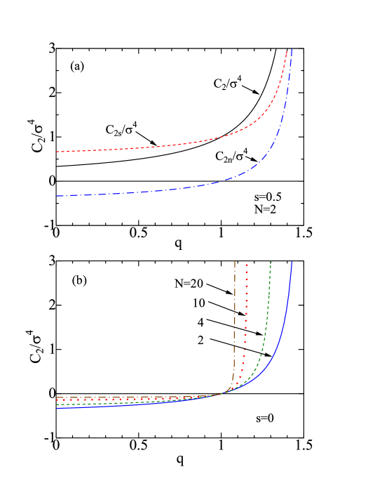
Figure 3: (Color online) (a) The $q$ dependence of $C_{2s}$ (the dashed curve), $C_{2n}$ (the dashed curve) and $C_{2}$ (=$C_{2s}+C_{2n}$, the solid curve) for $s=0.5$ and $N=2$. (b) The $q$ dependence of $C_{2}$ with $s=0$ for $N=2$ (the solid curve), 4 (the dotted curve), 10 (the dotted curve) and 20 (the chain curve).

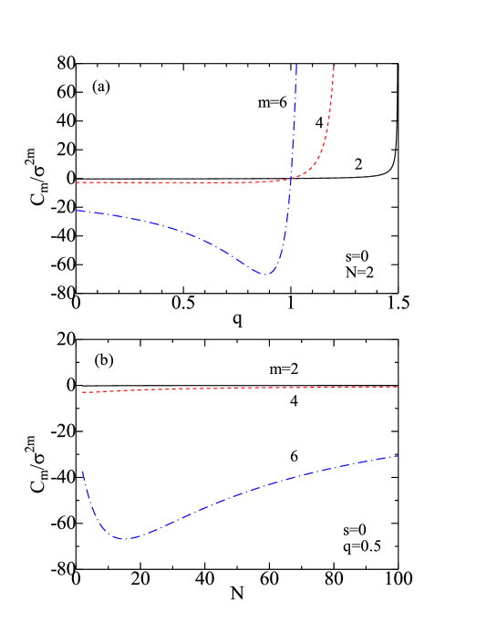
Figure 4: (Color online) (a) The $q$ dependence of $C_{m}$ with $N=2$ and (b) the $N$ dependence of $C_{m}$ with $q=0.5$ ($s=0$): $m=2$ (the solid curve), 4 (the dashed curve) and 6 (the chain curve).

Figure 3(a) shows the $q$ dependence of $C_{2s}$, $C_{2n}$ and $C_{2}$ ($=C_{2s}+C_{2n}$) for $s=0.5$ and $N=2$. We note that $C_{2s}\geq 0$, while $C_{2n}<0$ for $q<1.0$ and $C_{2n}\geq 0$ for $q\geq 1.0$. The $q$ dependences of $C_{2}$ for $s=0.0$ with $N=2$, 4, 10 and 20 are plotted in Fig.3(b), where $C_{2}$ vanishes for $q=1.0$, and it is $-0.33$, $-0.25$, $-0.14$ and $-0.083$ for $N=2$, 4, 10 and 20, respectively, at $q=0.0$. Figure 4(a) and 4(b) show the $q$- and $N$-dependent $C_{m}$, respectively, for $m=2$, 4 and 6 with $s=0.0$. Magnitudes of $C_{m}$ are significantly increased with increasing $m$.

III Discussion

III.1 PDF in the superstatistics

The physical origin of the correlation induced by nonextensivity is easily understood in the superstatistics. We consider the $N$-unit Langevin model subjected to additive noise given by Hasegawa08b

$$\frac{dx_{i}}{dt} = -\lambda x_{i}+\sqrt{2D}\>\xi_{i}(t)+I\hskip 28.45274pt\mbox{for $i=1$ to $N$},$$ (74)

where $\lambda$ denotes the relaxation rate, $\xi_{i}(t)$ the white Gaussian noise with the intensity $D$, and $I$ an external input. The PDF of $\pi^{(N)}(\mbox{\boldmath$x$})$ for the system is given by

$$\pi^{(N)}(\mbox{\boldmath$x$}) = \prod_{i=1}^{N}\>\pi^{(1)}(x_{i}),$$ (75)

where the univariate PDF of $\pi^{(1)}(x_{i})$ obeys the Fokker-Planck equation,

$$\frac{\partial\pi^{(1)}(x_{i},t)}{\partial t} = \frac{\partial}{\partial x_{i}}[(\lambda x_{i}-I)\pi^{(1)}(x_{i},t)]+D\frac{\partial^{2}}{\partial x_{i}^{2}}\pi^{(1)}(x_{i},t).$$ (76)

The stationary PDF of $\pi^{(1)}(x_{i})$ is given by

$$\pi^{(1)}(x_{i}) = \frac{1}{\sqrt{2\pi\sigma^{2}}}\exp\left(-\frac{(x_{i}-\mu)^{2}}{2\sigma^{2}}\right),$$ (77)

with

$$\mu=I/\lambda,\;\;\sigma^{2}=D/\lambda.$$ (78)

After the concept in the superstatistics Wilk00 ; Beck01 ; Beck05 ; Beck07 , we assume that a model parameter of $\tilde{\beta}$ ($\equiv\lambda/D$) fluctuates, and that its distribution is expressed by the $\chi^{2}$-distribution with rank $n$ Wilk00 ; Beck01 ,

$$f(\tilde{\beta}) = \frac{1}{\Gamma(n/2)}\left(\frac{n}{2\beta_{0}}\right)^{n/2}\tilde{\beta}^{n/2-1}e^{-n\tilde{\beta}/2\beta_{0}},$$ (79)

where $\Gamma(x)$ is the gamma function. Average and variance of $\tilde{\beta}$ are given by $\langle\tilde{\beta}\rangle_{\tilde{\beta}}=\beta_{0}$ and $(\langle\tilde{\beta}^{2}\rangle_{\tilde{\beta}}-\beta_{0}^{2})/\beta_{0}^{2}=2/n$, respectively. Taking the average of $\pi^{(N)}(\mbox{\boldmath$x$})$ over $f(\tilde{\beta})$, we obtain the stationary PDF given by Hasegawa09

$$p_{q}^{(N)}(\mbox{\boldmath$x$}) = \int_{0}^{\infty}\pi^{(N)}(\mbox{\boldmath$x$})\>f(\tilde{\beta})\>d\tilde{\beta},$$ (80)

$$= \frac{1}{Z_{q}^{(N)}}\exp_{q}\left[-\left(\frac{\beta_{0}}{2\nu_{q}^{(N)}}\right)\sum_{i=1}^{N}(x_{i}-\mu)^{2}\right],$$ (81)

with

$$Z_{q}^{(N)} = \>\left[\frac{2\nu_{q}^{(N)}}{(q-1)\beta_{0}}\right]^{N/2}\;\prod_{i=1}^{N}B\left(\frac{1}{2},\frac{1}{q-1}-\frac{i}{2}\right),$$ (82)

$$q = 1+\frac{2}{(N+n)},$$ (83)

where $\nu_{q}^{(N)}$ is given by Eq. (31). In the limit of $n\rightarrow\infty$ ($q\rightarrow 1.0$) where $f(\tilde{\beta})\rightarrow\delta(\tilde{\beta}-\beta_{0})$, the PDF reduces to the multivariate Gaussian distribution given by

$$p_{q}^{(N)}(\mbox{\boldmath$x$}) = \frac{1}{(Z_{1}^{(1)})^{N}}\prod_{i=1}^{N}\exp\left[-\frac{\beta_{0}}{2}\>(x_{i}-\mu)^{2}\right],$$ (84)

which agrees with Eqs. (75) and (77) for $\beta_{0}=\lambda/D=1/\sigma^{2}$.

We note that the PDF given by Eq. (81) is equivalent to that given by Eq. (34) derived by the MEM when we read $\beta_{0}=1/\sigma^{2}$. The nonextensivility-induced correlation arises from the common fluctuating field of $\tilde{\beta}$, because $p_{q}^{(N)}(\mbox{\boldmath$x$})\neq\prod_{i}p_{q}^{(1)}(x_{i})$ for $q\neq 1.0$ despite $\pi^{(N)}(\mbox{\boldmath$x$})=\prod_{i}\pi^{(1)}(x_{i})$.

III.2 PDF for classical ideal gas

It is worthwhile to discuss the PDF of one-dimensional ideal gas, whose hamiltonian is given by

$$H=\sum_{i=1}^{N}\>h_{i}=\sum_{i=1}^{N}\>\frac{p_{i}^{2}}{2m},$$ (85)

$m$ and $p_{i}$ standing for the mass and momentum, respectively, of ideal gas. By employing the OLM-MEM Martinez00 , we obtain the PDF given by (for details, see Appendix B)

$$p_{q}^{(N)}(\mbox{\boldmath$p$}) = \frac{1}{Z_{q}^{(N)}}\exp_{q}\left[-\left(\frac{\beta}{\nu_{q}^{(N)}}\right)\sum_{i=1}^{N}\>\frac{p_{i}^{2}}{2m}\right],$$ (86)

with

$$Z_{q}^{(N)}=\left\{\begin{array}[]{ll}\left[\frac{2\pi\>m\>\nu_{q}^{(N)}}{(q-1)\beta}\right]^{N/2}\frac{\Gamma\left(\frac{1}{q-1}-\frac{N}{2}\right)}{\Gamma\left(\frac{1}{q-1}\right)}&\mbox{for $1<q<3$},\\ \left(\frac{2\pi\>m}{\beta}\right)^{N/2}&\mbox{for $q=1$},\\ \left[\frac{2\pi m\>\nu_{q}^{(N)}}{(1-q)\beta}\right]^{N/2}\frac{\Gamma\left(\frac{1}{1-q}+1\right)}{\Gamma\left(\frac{1}{1-q}+1+\frac{N}{2}\right)}&\mbox{for $q<1$}.\\ \end{array}\right.$$ (90)

The internal energy is given by $U=N/2\beta$ [Eq. (B7)] independently of $q$, which yields the Dulong-Petit specific heat as in the Boltzmann-Gibbs statistics. The PDF of nonextensive ideal gas was originally discussed in Ref. Abe99 with the use of the normalized MEM Tsallis98 . Later it was re-examined by the OLM-MEM Martinez00 Abe01 . The PDF given by Eq. (86) is equivalent with the $q$-Gaussian PDF given by Eq. (34), if we read $m/\beta\rightarrow\sigma^{2}$.

III.3 PDF for classical harmonic oscillator

Next we consider the one-dimensional $N$-unit harmonic oscillators whose hamiltonian is given by

$$H=\sum_{i=1}^{N}\>h_{i}=\sum_{i=1}^{N}\>\left(\frac{p_{i}^{2}}{2m}+\frac{m\omega^{2}x_{i}^{2}}{2}\right),$$ (91)

$m$, $\omega$, $x_{i}$ and $p_{i}$ expressing the mass, oscillator frequency, position and momentum, respectively. With the use of the OLM-MEM Martinez00 , the PDF is given by (for details, see Appendix C)

$$p_{q}^{(N)}(\mbox{\boldmath$p$},\mbox{\boldmath$x$}) = \frac{1}{Z_{q}^{(N)}}\exp_{q}\left[-\left(\frac{\beta}{\nu_{q}^{(2N)}}\right)\sum_{i=1}^{N}\>\left(\frac{p_{i}^{2}}{2m}+\frac{m\omega^{2}x_{i}^{2}}{2}\right)\right],$$ (92)

with

$$Z_{q}^{(N)} = \left\{\begin{array}[]{ll}\left[\frac{2\pi\>\nu_{q}^{(2N)}}{(q-1)\omega\beta}\right]^{N}\frac{\Gamma\left(\frac{1}{q-1}-N\right)}{\Gamma\left(\frac{1}{q-1}\right)}&\mbox{for $1<q<3$},\\ \left(\frac{2\pi}{\omega\beta}\right)^{N}&\mbox{for $q=1$},\\ \left[\frac{2\pi\>\nu_{q}^{(2N)}}{(1-q)\omega\beta}\right]^{N}\frac{\Gamma\left(\frac{1}{1-q}+1\right)}{\Gamma\left(\frac{1}{1-q}+1+N\right)}&\mbox{for $q<1$},\\ \end{array}\right.$$ (96)

where $\nu_{q}^{(2N)}=(N+1)-Nq$ [Eq. (31)]. The internal energy is given by $U=N/\beta$ [Eq. (C7)], which is the same as that in Liyan08 and in the Boltzmann-Gibbs statistics. The PDF of the harmonic oscillator was calculated by using un-normalized Curado91 and normalized Tsallis98 MEMs in Ref.Lenzi01 , where $U$ has rather complicated $q$ and $N$ dependences (see Eqs. (12) and (22) of Ref. Lenzi01 ).

PDFs for classical ideal gas [Eqs. (86)] and harmonic oscillator [Eq. (92)] have the same structure as the $q$-Gaussian PDF given by Eq. (34), and they are expected to have the same properties as the $q$-Gaussian PDF. Actually correlation defined by $\langle h_{i}h_{j}\rangle_{q}-\langle h_{i}\rangle_{q}\langle h_{j}\rangle_{q}$ ($i\neq j$) is shown to be induced by nonextensivity in ideal gas Abe99b ; Liyan08 ; Feng10 and harmonic oscillator Feng10 .

III.4 $q$-product PDF

From functional forms of PDFs in Eq. (B3) or (C3), we expect that $p_{q}^{(N)}(\mbox{\boldmath$x$})$ may be expressed by

$$p_{q}^{(N)}(\mbox{\boldmath$x$}) = p_{q}^{(1)}(x_{1})\otimes_{q}p_{q}^{(1)}(x_{2})\otimes_{q}\cdot\cdot\otimes_{q}\>p_{q}^{(1)}(x_{N}),$$ (97)

where the $q$-product ($\otimes_{q}$) is defined by Borges04

$$x\otimes_{q}y = [x^{1-q}+y^{1-q}-1]^{1/(1-q)}.$$ (98)

Equation (97), however, does not hold when we take into account the precise form of PDFs including their normalization factors. For example, for a univariate PDF given by

$$p_{q}^{(1)}(x) = \frac{1}{X_{q}^{(1)}}[1-(1-q)\beta h_{1}]^{1/(1-q)},$$ (99)

with

$$X_{q}^{(1)} = {\rm Tr}_{1}\;[1-(1-q)\beta h_{1}]^{1/(1-q)},$$ (100)

Eqs. (97) and (99) yield the $q$-product PDF for $N=2$,

$$p_{q}^{(1)}(x_{1})\otimes_{q}p_{q}^{(1)}(x_{2}) = \frac{1}{(X_{q}^{(1)})^{1-q}}\left[2-(X_{q}^{(1)})^{1-q}-(1-q)\beta(h_{1}+h_{2})\right]^{1/(1-q)}.$$ (101)

Unfortunately, Eq. (101) is not in agreement with the bivariate PDF given by

$$p_{q}^{(2)}(x_{1},x_{2}) = \frac{1}{X_{q}^{(2)}}[1-(1-q)\beta(h_{1}+h_{2})]^{1/(1-q)},$$ (102)

$$\neq p_{q}^{(1)}(x_{1})\otimes_{q}p_{q}^{(1)}(x_{2}),$$ (103)

with

$$X_{q}^{(2)} = {\rm Tr}_{12}\;[1-(1-q)\beta(h_{1}+h_{2})]^{1/(1-q)}.$$ (104)

It is easy to see that the relation: $p_{q}^{(2)}(x_{1},x_{2})=p_{q}^{(1)}(x_{1})\otimes_{q}p_{q}^{(1)}(x_{2})$ holds only for $X_{q}^{(1)}=X_{q}^{(2)}=1$ in Eqs. (101) and (102).

IV Concluding remarks

It has been postulated that the Tsallis entropy $S_{q}^{(N)}$ satisfies the pseudoadditivity given by Eq. (3) or (5), and that the factorized PDF: $p_{q}^{(N)}(\mbox{\boldmath$x$})=\prod_{i}p_{q}^{(1)}(x_{i})$ leads to the Tsallis entropy expressed by Eq. (1) Tsallis01 . The pseudoadditivity is a basis of the Tsallis entropy and detailed discussions on its pseudoadditivity have been made Tsallis01 ; Raj99 ; Abe00 ; Abe01b . We should note, however, that this is not self-consistent because the PDF derived by the MEM for $S_{q}^{(N)}$ leads to $p_{q}^{(N)}(\mbox{\boldmath$x$})\neq\prod_{i}p_{q}^{(1)}(x_{i})$ which contradicts with the postulated, factorized PDF. The pseudoadditivity cannot be a basis of the Tsallis entropy Lavenda05 .

It has been also controversial whether the $statistical$ $independence$ is expressed by (a) $p_{q}^{(N)}(\mbox{\boldmath$x$})=\prod_{i}p_{q}^{(1)}(x_{i})$ or (b) $H=\sum_{i}h_{i}$ in nonextensive systems Wang02 ; Wang02b ; Jiulin09 . If we assume that the condition (a) expresses the statistical independence of $N$-unit subsystems, we obtain $S_{q}^{(N)}=S_{q,FA}^{(N)}$ which satisfies the pseudoadditivity. However, the PDF derived by the MEM for $S_{q}^{(N)}$ yields $p_{q}^{(N)}(\mbox{\boldmath$x$})\neq\prod_{i}p_{q}^{(1)}(x_{i})$, which is inconsistent with the assumption. This means that the statistical independence cannot be expressed by neither the product nor $q$-product PDFs.

Our calculations with the use of the multivariate $q$-Gaussian PDF have shown that

(i) the Tsallis entropy is given by $S_{q}^{(N)}=S_{q,FA}^{(N)}+\Delta S_{q}^{(N)}\geq S_{q,FA}^{(N)}$ where the correction term of $\Delta S_{q}^{(N)}$ is significant for large $|q-1|$ and/or large $N$,

(ii) the Tsallis entropy does not satisfy pseudoadditivity, and

(iii) nonextensivity-induced correlation is realized in higher-order correlations $C_{m}$ for $m\geq 2$ while $C_{1}$ expresses the intrinsic correlation.

The items (i)-(iii) are expected to hold also for classical ideal gas and harmonic oscillator. The item (ii) is against the common wisdom Lavenda05 . The nonextensivity-induced correlation in the item (iii) is elucidated as arising from common fluctuating field introduced in the superstatistics Wilk00 ; Beck01 ; Beck05 . It has been shown that the FA is not a good approximating method in classical nonextensive systems, just as in quantum ones as recently pointed out in Refs. Hasegawa09b ; Hasegawa09c . We should be careful in adopting the FA, although it has been widely employed in many applications of the classical and quantum nonextensive statistics Nonext .

*

Appendix A A. Evaluations of $q$-averages

We briefly discuss evaluations of $q$-averages given by

$$Z_{q}^{(N)}(\alpha) = \int\>\left[1-(1-q)\alpha\>\Phi(\mbox{\boldmath$x$})\right]^{1/(1-q)}\>d\mbox{\boldmath$x$},$$ (A1)

$$Q_{q}^{(N)}(\alpha) = \langle Q(\mbox{\boldmath$x$})\rangle_{q}=\frac{1}{\nu_{q}^{(N)}Z_{q}^{(N)}}\int\>Q(\mbox{\boldmath$x$})\>\left[1-(1-q)\alpha\>\Phi(\mbox{\boldmath$x$})\right]^{q/(1-q)}\>d\mbox{\boldmath$x$},$$ (A2)

by using the exact expressions for the gamma function Prato95 ; Rajagopal98 ; Hasegawa09b :

$$y^{-s} = \frac{1}{\Gamma(s)}\int_{0}^{\infty}u^{s-1}e^{-yu}\>du\hskip 56.9055pt\mbox{for $s>0$},$$ (A3)

$$y^{s} = \frac{i}{2\pi}\Gamma(s+1)\int_{C}(-t^{-s-1})e^{-yt}\>dt\hskip 28.45274pt\mbox{for $s>0$},$$ (A4)

where $\alpha=1/(2\nu_{q}^{(N)}\sigma^{2})$, $\Phi(\mbox{\boldmath$x$})$ is given by Eq. (23), $Q(\mbox{\boldmath$x$})$ denotes an arbitrary function of $x$, $C$ the Hankel path in the complex plane, and Eq. (39) being employed. We obtain Prato95 ; Rajagopal98 ; Hasegawa09b

$$Z_{q}^{(N)}(\alpha) = \left\{\begin{array}[]{ll}\frac{1}{\Gamma\left[\frac{1}{q-1}\right]}\int_{0}^{\infty}u^{\frac{1}{q-1}-1}e^{-u}Z_{1}^{(N)}[(q-1)\alpha u]\>du&\mbox{for $q>1.0$},\\ \frac{i}{2\pi}\Gamma\left[\frac{1}{1-q}+1\right]\int_{C}(-t)^{-\frac{1}{1-q}-1}e^{-t}Z_{1}^{(N)}[-(1-q)\alpha t]\>dt&\mbox{for $q<1.0$},\end{array}\right.$$ (A7)

$$Q_{q}^{(N)}(\alpha) = \left\{\begin{array}[]{ll}\frac{1}{\nu_{q}^{(N)}Z_{q}^{(N)}\Gamma\left[\frac{q}{q-1}\right]}\int_{0}^{\infty}u^{\frac{q}{q-1}-1}e^{-u}Z_{1}^{(N)}[(q-1)\alpha u]\>Q_{1}^{(N)}[(q-1)\alpha u]\>du&\mbox{for $q>1.0$},\\ \frac{i}{2\pi\nu_{q}^{(N)}Z_{q}^{(N)}}\Gamma\left[\frac{q}{1-q}+1\right]\int_{C}(-t)^{-\frac{q}{1-q}-1}e^{-t}Z_{1}^{(N)}[-(1-q)\alpha t]\\ \hskip 56.9055pt\times\>Q_{1}^{(N)}[-(1-q)\alpha t]\>dt&\mbox{for $q<1.0$},\end{array}\right.$$ (A12)

where

$$Z_{1}^{(N)}(\alpha) = \int e^{-\alpha\>\Phi(\mbox{\boldmath$x$})}\>d\mbox{\boldmath$x$},$$ (A14)

$$Q_{1}^{(N)}(\alpha) = \frac{1}{Z_{1}^{(N)}(\alpha)}\int\>Q(\mbox{\boldmath$x$})\>e^{-\alpha\>\Phi(\mbox{\boldmath$x$})}\>d\mbox{\boldmath$x$}.$$ (A15)

Thus we may evaluate the $q$ average of $Q(\mbox{\boldmath$x$})$ from its average over the Gaussian PDF.

For example, by using the relations for $N=2$,

$$\langle(x_{i}-\mu)^{2}\rangle_{1} = \frac{1}{2\alpha},$$ (A16)

$$\langle(x_{i}-\mu)(x_{j}-\mu)\rangle_{1} = \frac{s}{2\alpha}\hskip 56.9055pt\mbox{for $i\neq j$}$$ (A17)

$$\langle(x_{i}-\mu)^{2}(x_{j}-\mu)^{2}\rangle_{1} = \frac{1+2s^{2}}{4\alpha^{2}}\hskip 28.45274pt\mbox{for $i\neq j$},$$ (A18)

and employing Eqs. (LABEL:eq:X1) and (LABEL:eq:X2), we obtain

$$\langle(x_{i}-\mu)^{2}\rangle_{q} = \sigma^{2},$$ (A19)

$$\langle(x_{i}-\mu)(x_{j}-\mu)\rangle_{q} = \sigma^{2}s\hskip 142.26378pt\mbox{for $i\neq j$},$$ (A20)

$$\langle(x_{i}-\mu)^{2}(x_{j}-\mu)^{2}\rangle_{q} = \frac{(N+2-Nq)(1+2s^{2})\>\sigma^{4}}{(N+4)-(N+2)q}\hskip 28.45274pt\mbox{for $i\neq j$},$$ (A21)

which yield Eqs. (52)-(54) and (59).

Appendix B B. PDF for ideal gas

In order to obtain the PDF of $p_{q}^{(N)}(\mbox{\boldmath$p$})$ for classical ideal gas with the OLM-MEM Martinez00 , we impose the constraints given by

$$1 = \int p_{q}^{(N)}(\mbox{\boldmath$p$})\>d\mbox{\boldmath$p$},$$ (B1)

$$U = \sum_{i=1}^{N}\left<\frac{p_{i}^{2}}{2m}\right>_{q}.$$ (B2)

The OLM-MEM Martinez00 yields

$$p_{q}^{(N)}(\mbox{\boldmath$p$}) \propto \left[1-(1-q)\beta\left(\sum_{i=1}^{N}\>\frac{p_{i}^{2}}{2m}-U\right)\right]^{1/(1-q)},$$ (B3)

where the Lagrange multiplier $\beta$ expresses the inverse of temperature. Rewriting Eq. (B3) as

$$p_{q}^{(N)}(\mbox{\boldmath$p$}) \propto \left[1-(1-q)\alpha\>\sum_{i=1}^{N}\>\frac{p_{i}^{2}}{2m}\right]^{1/(1-q)},$$ (B4)

with

$$\alpha = \frac{\beta}{1+(1-q)\beta U},$$ (B5)

we obtain $U$ in terms of $\alpha$ as given by

$$U = \frac{N}{(N+2-Nq)\alpha}.$$ (B6)

From Eqs. (B5) and (B6), $U$ and $\alpha$ are self-consistently determined as

$$U = \frac{N}{2\beta},$$ (B7)

$$\alpha = \frac{2\beta}{N+2-Nq}.$$ (B8)

With the use of Eqs. (B4), (B7) and (B8), the PDF is given by Eqs. (86) and (90).

Appendix C C. PDF for harmonic oscillators

We obtain the PDF for classical harmonic oscillators with the OLM-MEM Martinez00 , imposing the constraints given by

$$1 = \int\int p_{q}^{(N)}(\mbox{\boldmath$p$},\mbox{\boldmath$x$})\>d\mbox{\boldmath$p$}\>d\mbox{\boldmath$x$},$$ (C1)

$$U = \sum_{i=1}^{N}\left<\frac{p_{i}^{2}}{2m}+\frac{m\omega^{2}x_{i}^{2}}{2}\right>_{q}.$$ (C2)

The OLM-MEM Martinez00 leads to

$$p_{q}^{(N)}(\mbox{\boldmath$p$},\mbox{\boldmath$x$}) \propto \left[1-(1-q)\beta\left(\sum_{i=1}^{N}\>\left(\frac{p_{i}^{2}}{2m}+\frac{m\omega^{2}x_{i}^{2}}{2}\right)-U\right)\right]^{1/(1-q)},$$ (C3)

which is rewritten as

$$p_{q}^{(N)}(\mbox{\boldmath$p$},\mbox{\boldmath$x$}) \propto \left[1-(1-q)\alpha\>\sum_{i=1}^{N}\left(\>\frac{p_{i}^{2}}{2m}+\frac{m\omega^{2}x_{i}^{2}}{2}\right)\right]^{1/(1-q)},$$ (C4)

with

$$\alpha = \frac{\beta}{1+(1-q)\beta U}.$$ (C5)

We obtain $U$ in terms of $\alpha$ as given by

$$U = \frac{N}{(N+1-Nq)\alpha}.$$ (C6)

From Eqs. (C5) and (C6), $U$ and $\alpha$ are self-consistently determined as

$$U = \frac{N}{\beta},$$ (C7)

$$\alpha = \frac{\beta}{N+1-Nq}.$$ (C8)

By using Eqs. (C4), (C7) and (C8), we finally obtain the PDF given by Eqs. (92) and (96).

References

- (1) C. Tsallis: J. Stat. Phys. 52, 479 (1988).
- (2) C. Tsallis, R. S. Mendes, and A. R. Plastino: Physica A 261, 534 (1998).
- (3) C. Tsallis, in Nonextensive Statistical Mechanics and Its Application, edited by S. Abe and Y. Okamoto (Springer-Verlag, Berlin, 2001), p 3.
- (4) C. Tsallis: Physica D 193, 3 (2004).
- (5) E. M. F. Curado and C. Tsallis, J. Phys. A 24 (1991) L69; 24, 3187 (1991); 25, 1019 (1992).
- (6) S. Martinez, F. Nicolas, F. Pennini, and A. Plastino, Physica A 286, 489 (2000).
- (7) G. L. Ferri, S. Martinez, and A. Plastino, J. Stat. Mech. Theory Exp., p04009 (2005).
- (8) Q. A. Wang, M. Pezeril, L. Nivanen, and A. L. Méhauté, Chaos, Solitons and Fractals 13, 131 (2002).
- (9) Q. A. Wang, Physics Lettrs A 300, 169 (2002).
- (10) D. Jiulin, arXiv:0906.1409
- (11) E. K. Lenzi, R. S. Mendes, L. R. da Silva, and L. C. Malacarne, Physica A 289, 44 (2001).
- (12) H. Hasegawa, Phys. Rev. E 78, 021141 (2008).
- (13) H. Hasegawa, Phys. Rev. E 80, 051125 (2009).
- (14) S. Abe, Physica A 269, 403 (1999).
- (15) L. Liyan and D. Jiulin, Physica A 387, 5417 (2008).
- (16) Zhi-Hui Feng and Li-Yan Liu, Physica A 389, 237 (2010).
- (17) G. Wilk and Z. Wlodarczyk, Phys. Rev. Lett. 84, 2770 (2000).
- (18) C. Beck, Phys. Rev. Lett. 87, 180601 (2001).
- (19) C. Beck and E. G. D. Cohen, Physica A 322, 267 (2003).
- (20) C. Beck, arXiv:0705.3832.
- (21) E. P. Borges, Physica A 340, 95 (2004).
- (22) D. Prato, Phys. Lett. A 203, 165 (1995).
- (23) A. K. Rajagopal, R. S. Mendes and E. K. Lenzi, Phys. Rev. Lett. 80, 3907 (1998).
- (24) S. Abe, Phys. Rev. E 66, 046134 (2002).
- (25) S. Abe, Phys. Lett. A 263, 424 (1999); 267, 456 (2000)[E].
- (26) S. Abe, S. Martinez, F. Pennini, and A. Plastino, Physics Letters A 278, 249 (2001).
- (27) A. K. Rajagopal and S. Abe, Phys. Rev. Lett. 83, 1711 (1999).
- (28) S. Abe, Phys. Lett. A 271, 74 (2000).
- (29) S. Abe, Phys. Rev. E 63, 061105 (2001).
- (30) B. H. Lavenda and J. Dunning-Davies, J. Appl. Sci. 5, 920 (2005).
- (31) H. Hasegawa, Phys. Rev. E 80, 011126 (2009).
- (32) H. Hasegawa, arXiv:09060225.
-
(33)
Lists of many applications of the nonextensive
statistics are available at
URL:
(http://tsallis.cat.cbpf.br/biblio.htm)