Particle hydrodynamics with tessellation techniques

Abstract

Lagrangian smoothed particle hydrodynamics (SPH) is a well-established approach to model fluids in astrophysical problems, thanks to its geometric flexibility and ability to automatically adjust the spatial resolution to the clumping of matter. However, a number of recent studies have emphasized inaccuracies of SPH in the treatment of fluid instabilities. The origin of these numerical problems can be traced back to spurious surface effects across contact discontinuities, and to SPH’s inherent prevention of mixing at the particle level. We here investigate a new fluid particle model where the density estimate is carried out with the help of an auxiliary mesh constructed as the Voronoi tessellation of the simulation particles instead of an adaptive smoothing kernel. This Voronoi-based approach improves the ability of the scheme to represent sharp contact discontinuities. We show that this eliminates spurious surface tension effects present in SPH and that play a role in suppressing certain fluid instabilities. We find that the new ‘Voronoi Particle Hydrodynamics’ described here produces comparable results than SPH in shocks, and better ones in turbulent regimes of pure hydrodynamical simulations. We also discuss formulations of the artificial viscosity needed in this scheme and how judiciously chosen correction forces can be derived in order to maintain a high degree of particle order and hence a regular Voronoi mesh. This is especially helpful in simulating self-gravitating fluids with existing gravity solvers used for N-body simulations.

1 Introduction

Numerical simulations have become an important research tool in many areas of astrophysics, in particular in cosmic structure formation and galaxy formation. This is in part because the physical conditions involved cannot be reproduced in laboratories on Earth, so that simulations serve as a replacement for experiments. Perhaps more importantly, simulations in principle allow a full modeling of all the involved physics. However, a significant problem in practice is that that the equations one wants to solve first have to be numerically discretized in a suitable fashion. The accuracy of simulations depends strongly on the properties of this discretization, and it hence remains an important task to find improved numerical schemes for astrophysical applications.

In cosmic structure formation, matter is initially essentially uniformly distributed, but clusters with time under the action of self-gravity to enormous density contrasts, producing galaxies of vastly different sizes. Given the variety of involved geometries, densities and velocities, it is clear that a Lagrangian method, where the mass of a resolution element stays (roughly) constant, would be most convenient. This is because a Lagrangian method automatically concentrates the resolution in regions where the galaxies form, and hence focuses the numerical effort on the regions of interest. On the other hand, traditional mesh-based approaches to hydrodynamics, so-called Eulerian methods, discretize the volume in a set of cells and do not follow the clustering of matter, unless this is attempted with a suitable adaptive mesh-refinement strategy.

The by far most widely used Lagrangian approach in structure formation is smoothed particle hydrodynamics (SPH, as reviewed by Monaghan, 1992, 2005; Rosswog, 2009), a technique that dates back to particle-based approaches first developed in astronomy more than 30 years ago (Lucy, 1977; Gingold & Monaghan, 1977; Larson, 1978). In this method the fluid is discretized in terms of particles of fixed mass, which are used to construct an approximation to the Euler equations based on the adaptive kernel interpolation technique. SPH can be very easily coupled to self-gravity, it is remarkably robust (e.g. negative densities cannot arise), and the introduction of extra physics (e.g. feedback processes in the context of star formation) is intuitive. All of these properties have made it very popular for problems such as planet formation or galaxy mergers (e.g. Mihos & Hernquist, 1996; Mayer et al., 2002; Robertson et al., 2004; Dolag et al., 2005), where spatially separated regions of the simulation volume feature widely different densities.

However, recent studies have highlighted a number of differences in the results of SPH-based calculations compared to more traditional grid-based Eulerian methods for hydrodynamics. For example, the two methods appear to disagree about the entropy produced in the central region of a forming galaxy cluster under non-radiative conditions, as first seen in the ‘Santa Barbara cluster comparison project’ (Frenk et al., 1999). It has been suggested that this problem may be caused by a suppression of the Raleigh-Taylor fluid instability in SPH (Mitchell et al., 2009) and the lack of mixing at the particle level (Tasker et al., 2008; Wadsley et al., 2008). Indeed, Agertz et al. (2007) have shown that SPH tends to suppress Kelvin-Helmholtz fluid instabilities in shear flows across interfaces with sizable density jumps. In such a situation, SPH’s density estimate leads to spurious forces at the interface which produce an artificial ‘gap’ in the particle distribution and a surface tension effect that ultimately produces errors in the hydrodynamical evolution. To what extent these numerical artifacts negatively affect the global accuracy of simulations in practice is unclear, and this can in any case be expected to be problem dependent. However, an improvement of standard SPH that avoids these errors is obviously desirable.

First proposals in this direction have recently been made. Price (2008) suggests to introduce artificial heat conduction into SPH such that discontinuities in the temperature field are smoothed out, in analogy to the ordinary artificial viscosity that effectively smoothes out discontinuities in the velocity field occurring at shocks. This heat conduction produces a soft instead of an abrupt transition of the specific entropy across a contact discontinuity, which in turn helps to better represent the growth of Kelvin-Helmholtz instabilities at such interfaces. More recently, Read et al. (2009) have modified an idea by Ritchie & Thomas (2001) for a modified SPH density estimate that assumes that the local neighbours have similar pressures, and which is designed to avoid the ‘pressure blip’ in the standard approach at contact discontinuities. Together with a modified kernel shape and a drastically enlarged number of neighbours (by a factor of $\sim 10$, implying a similar increase in the computational cost), Read et al. (2009) obtained better growth of Kelvin-Helmholtz instabilities across density jumps.

In this work we follow a different approach that eliminates the ordinary SPH kernel altogether. Instead, we use the distribution of points with variable masses to construct an auxiliary mesh, which is then used to derive local density estimates. If the particle hydrodynamics is derived from a Lagrangian, it turns out that obtaining this density estimate is already sufficient to uniquely determine the equations of motion. The use of Delaunay tessellations to construct density fields from arbitrary point sets has been discussed in the literature (Schaap & van de Weygaert, 2000a; Icke & van de Weygaert, 1987; van de Weygaert & Icke, 1989; Pelupessy et al., 2003), but as we show in this paper, its topological dual, the Voronoi tessellation, is actually preferable for our hydrodynamical application. In the Voronoi tessellation, to every particle a polyhedra is assigned which encompasses the space closer to this particle than to any other. Based on these volumes associated with each particle, local densities and hydrodynamical forces can be estimated, leading to an interesting alternative to SPH. In particular, it is immediately clear that unlike SPH this approach yields a consistent discretization not only of the mass but also of the volume, which should help to yield an improved representation of contact discontinuities. We note that a conceptionally similar approach to Voronoi based particle hydrodynamics was first discussed by Serrano & Español (2001) in the context of a mesoscopic fluid particle model. We here extend this idea to the treatment of the Euler equations in astrophysical systems.

We emphasize that the method we introduce in this study is radically different from to the one implemented in the new AREPO code (Springel, 2009). Whereas the latter is also based on a (moving) Voronoi tessellation, it employs a finite volume scheme with a Riemann solver to compute hydrodynamical fluxes across mesh boundaries. This involves an explicit second-order reconstruction of the fluid throughout the volume, and allows for changes of the mass contained in each cell even if the mesh is on average moving with the flow. In contrast, we here derive a fluid particle model from a discretized Lagrangian in which the masses of each element stay strictly constant, and in which the motion of the particles is governed by pairwise pressure force exchanged between them. While AREPO is conceptually close to the techniques used in Eulerian hydrodynamics, the method we study here is conceptually close to SPH.

This paper is structured as follows. In Section 2, we discuss how the equations of motion can be derived for the Lagrangian particle approach to hydrodynamics discussed here. We will also present suitable formulations of artificial viscosity for our scheme. In Section 3, we discuss the role of the regularity of Voronoi cells and means to improve it. We briefly describe the implementation of our numerical scheme in a modified version of the GADGET code in Section 4, and then turn in Section 5 to a description of results for a suite of test problems with our new ‘Voronoi Particle Hydrodynamics’ (VPH) scheme. These tests range from simple shock-tube problems, to fluid instabilities, and three-dimensional stripping of gas in a supersonic flow. Finally, we summarize our conclusions in Section 6. In two Appendices, we discuss gradient operators for Voronoi meshes and give the derivation of correction forces that can be used to maintain very regular mesh geometries, if desired.

2 Particle based hydrodynamics

We begin by introducing our methodology for a particle-based fluid dynamics based on Voronoi tessellations. This method is close in spirit to SPH, but differs in important aspects. Where appropriate, we discuss these differences in detail.

2.1 A Lagrangian approach for particle based fluid dynamics

We discretize the fluid in terms of $N$ mass elements of mass $m_{i}$. The discretized fluid Lagrangian can then be adopted as

$$L=\sum_{i}\left[\>\frac{1}{2}\>m_{i}\>{\mn@boldsymbol{v}}_{i}^{2}-m_{i}\>u_{i}(\rho_{i},s_{i})\>\right].$$ (1)

This is simply the difference of the kinetic and thermal energy of the particles. The thermal energy $u_{i}$ per unit mass depends both on the density $\rho_{i}$ and the specific entropy $s_{i}$ of the particle. In this work, we aim to approximate inviscid ideal gases, hence the equation of state (EOS) is that of a polytropic gas, where the pressure is $P_{i}=s_{i}\rho^{\gamma}$, and the entropic function $s_{i}$ (or simply ‘entropy’ for short, since it depends only on the thermodynamic entropy) labels the adiabat on which this gas element resides.

When the specific entropy $s_{i}$ and the mass $m_{i}$ remain constant for a fluid element $i$, the internal energy $u_{i}$ changes according to $\frac{\partial u}{\partial\rho}=\frac{P}{\rho^{2}}$. Using this result, we can readily write down the Lagrangian equations of motion of (reversible) fluid dynamics:

$$m_{i}\ddot{\mn@boldsymbol{r}}_{i} = -\sum_{j}^{N}m_{j}\frac{\partial u_{j}}{\partial{\mn@boldsymbol{r}}_{i}}$$ (2)

$$= -\sum_{j}^{N}m_{j}\frac{\partial u_{j}}{\partial\rho_{j}}\frac{\partial\rho_{j}}{\partial{\mn@boldsymbol{r}}_{i}}$$

$$= -\sum_{j}^{N}m_{j}\frac{P_{j}}{\rho_{j}^{2}}\frac{\partial\rho_{j}}{\partial V_{j}}\frac{\partial V_{j}}{\partial{\mn@boldsymbol{r}}_{i}}$$

We see that the primary input required for a more explicit form of the equations is a density estimate based on the particle coordinates, or alternatively, an estimate of the volume associated with a given particle.

SPH addresses this task with a kernel estimation technique to obtain the density, where an adaptive spherically symmetric smoothing kernel is employed to calculate the density based on the spatial distribution of an approximately fixed number of nearest neighbours. The Lagrangian then uniquely determines the equations of motion that simultaneously conserve energy and entropy (Springel & Hernquist, 2002). However, we note that SPH does not achieve a consistent volume estimate, i.e. the sum of the effective volumes of the particles, $V_{i}=m_{i}/\rho_{i}$, is not guaranteed to be equal to the total simulated volume. Furthermore, the inherent smoothing operation in the density estimate is bound to be inaccurate at contact discontinuities and phase interfaces, where the density may discontinuously jump by a large factor. In the following, we therefore look for alternative ways to construct density estimates which improve on these deficits.

2.2 Density estimates with tessellation techniques

One promising approach for more accurate density and specific volume estimates lies in the use of an auxiliary mesh that is generated by the particle distribution. A mesh can readily yield a partitioning of the volume such that the total volume is conserved, and also allows multiple ways to ‘spread out’ the particle masses $m_{i}$ in a conservative fashion such that an estimate of the density field is obtained.

There are two basic geometric constructions that suggest themselves as such mesh candidates. These are the Delaunay (Dirichlet, 1850) and the Voronoi tessellations (Voronoj, 1908), which are in fact mathematically closely related, as we discuss below. In the Voronoi tessellation, space is subdivided into non-overlapping polyhedra which each encompass the volume which is closer to its corresponding point than to any other point. The surfaces of these polyhedra are therefore the bisectors to the nearest neighbours. The Delaunay tessellation on the other hand decomposes space into a set of tetrahedra (or triangles in 2D), with vertices at the point coordinates. The defining property of the Delaunay tessellation is that the circumcircles of the tetrahedra do not contain any of the points in their interior. This property in fact makes this tessellation uniquely determined for points in general position.

It turns out that these two tessellations are dual to each other; to each edge of the Delaunay tessellation corresponds a face of the Voronoi tessellation, and the circumcircle centres of the Delaunay tetrahedra are the vertices of the Voronoi faces. One implication of this is that the Delaunay and Voronoi Tessellations can be easily transformed into each other. In practice it is typically simpler to always construct the Delaunay tessellation, even if one works with the Voronoi, because the former has more efficient and simpler algorithms for construction.

Both tessellations can in principle be used to derive density estimates. Schaap & van de Weygaert (2000b) introduced the Delaunay Tessellation Field Estimator (DTFE) technique, and Pelupessy et al. (2003) showed that it offers superior resolution compared to SPH-like density estimates for detecting cosmological large-scale structure (for a review see van de Weygaert & Schaap, 2009). In this approach, the total volume of the contiguous set of Delaunay cells around a point is used to assign particle densities, and a full density field can be constructed by linearly interpolating the densities inside each Delaunay tetrahedron. As a possible application of this density estimate, Pelupessy et al. (2003) also suggested its use in a particle-based hydrodynamic scheme. However, we caution that a rather serious short-coming of the Delaunay tessellation in this context is that the tessellation may occasionally change discontinuously as a function of the particle coordinates. This happens whenever a particle moves over the circumcircle of one of the tetrahedra. An infinitesimal particle motion can hence be sufficient to create finite changes in the volume of its associated contiguous Delaunay cell (this is the union of all Delaunay tetrahedra of which the given point is one of the vertices) of a particle. As a result, the thermal energy of the point set is not a continuous function of the particle coordinates. This makes the DTFE technique ill suited to be the basis of a hydrodynamical particle method.

On the other hand, the volumes of the Voronoi cells always depend continuously on the particle coordinates, despite the fact that topological changes of the tessellation may occur as a result of particle motion. This is because flips of edges in the Delaunay tessellation happen precisely when the corresponding Voronoi faces have vanishing area. Another advantage of the Voronoi tessellation is that it is always uniquely defined for any distribution of the points, whereas for certain degenerate point sets (those where more than four points lie on a common circumsphere), more than one valid Delaunay tessellation may exist, which can then make Delaunay-derived density estimates non-unique. We remark that the uniqueness of the Voronoi tessellation does not hold in reverse, i.e. a given Voronoi tessellation can in general be produced by a number of different point distributions. This has important consequences for the stability of the scheme, as we discuss later on in more detail.

Based on the above, the Voronoi tessellation is a promising construction for a particle fluid model, hence we adopt it in the following. In particular, we shall associate the volume $V_{i}$ of a Voronoi cell with its corresponding point, yielding a consistent decomposition of the total simulated volume. The simplest possible density estimate is then simply given by

$$\rho_{i}=\frac{m_{i}}{V_{i}}$$ (3)

which we shall use in this paper. More involved higher-order density field reconstructions could be considered as well, an idea we leave for future work.

Based on this density estimate, and given the specific entropies of each particle, the local pressure and the thermal pressure per unit mass can be computed. Also, one may define a gradient operator for the Voronoi mesh (see our discussion in Appendix A.1), which could be used to estimate pressure gradients, and hence to yield discretizations of the Euler equations. However, a better approach is to start from the discretized Lagrangian, as this automatically gives equations of motion that satisfy the conservation laws. We shall adopt this strategy in the following.

2.3 Equations of motion for Voronoi-based particle hydrodynamics

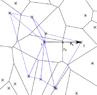
Figure 1: Section of a Voronoi diagram for a set of points marked with asterisks. All the triangles in the dual Delaunay tessellation that are shared by the point in the centre are marked in blue. The vectors ${\mn@boldsymbol{c}}_{ij}$ and ${\mn@boldsymbol{e}}_{ij}$ needed to calculate the derivative of the volume are also marked.

Since the volumes of the Voronoi cells depend only on the configuration of the points, we can readily obtain the equations of motion if we find the partial derivative of a cell volume with respect to any of the particle coordinates. We here adopt the result of Serrano & Español (2001), who showed that the relevant derivative is given by (see also De Fabritiis et al., 2006)

$$\frac{\partial V_{j}}{\partial{\mn@boldsymbol{r}}_{i}}=-A_{ij}\left(\frac{{\mn@boldsymbol{c}}_{ij}}{R_{ij}}+\frac{{\mn@boldsymbol{e}}_{ij}}{2}\right)\;\;\;\mbox{for $i\neq j$,}$$ (4)

where $\frac{\partial}{\partial{\mn@boldsymbol{r}}_{i}}$ denotes the gradient operator with respect to ${\mn@boldsymbol{r}}_{i}$. Here $R_{ij}$ is the distance between two neighboring points, ${\mn@boldsymbol{e}}_{ij}=({\mn@boldsymbol{r}}_{j}-{\mn@boldsymbol{r}}_{i})/R_{ij}$ denotes a unit vector from $i$ to the neighbour $j$, which is normal to the Voronoi face of area $A_{ij}$ between cells $i$ and $j$. Formally, we can define $A_{ij}$ for any pair of different particles, but if $i$ and $j$ are not neighbours in the Voronoi tessellation (i.e. do not share a face), we set $A_{ij}\equiv 0$, implying that in sums that involve the factor $A_{ij}$ only the direct neighbours contribute. Note that equation (4) holds only for $j\neq i$. But one can readily derive an expression for $\partial V_{i}/\partial{\mn@boldsymbol{r}}_{i}$ by invoking volume conservation. This yields

$$\frac{\partial V_{i}}{\partial{\mn@boldsymbol{r}}_{i}}=-\sum_{j\neq i}\frac{\partial V_{j}}{\partial{\mn@boldsymbol{r}}_{i}}.$$ (5)

As sketched in Figure 1, the vector ${\mn@boldsymbol{c}}_{ij}$ points from the midpoint between $i$ and $j$ to the centroid of the face $A_{ij}$, and is orthogonal to ${\mn@boldsymbol{e}}_{ij}$. The term involving ${{\mn@boldsymbol{e}}_{ij}}/{2}$ can be easily understood geometrically from the change of the volumes of the pair of pyramids spanned by the face between $i$ and $j$ and the two points. But if the center of the face is displaced from the line connecting $i$ and $j$, a second term involving ${\mn@boldsymbol{c}}_{ij}$ appears that stems from the turning of the face when the points are moved.

We are now in a position to write down the resulting equations of motion, based on equations (2), (4) and (5). This first yields

$$\frac{\partial\rho_{j}}{\partial{\mn@boldsymbol{r}}_{i}} = \frac{m_{j}}{V_{j}^{2}}\left[(1-\delta_{ij})A_{ij}\left(\frac{{\mn@boldsymbol{c}}_{ij}}{R_{ij}}+\frac{{\mn@boldsymbol{e}}_{ij}}{2}\right)\right.$$ (6)

$$-\delta_{ij}\sum_{k\neq j}A_{jk}\left.\left(\frac{{\mn@boldsymbol{c}}_{jk}}{R_{jk}}+\frac{{\mn@boldsymbol{e}}_{jk}}{2}\right)\right],$$

which then gives rise to the equations of motion in the form

$$m_{i}\ddot{\mn@boldsymbol{r}}_{i}=\sum_{j\neq i}A_{ij}(P_{i}-P_{j})\left(\frac{{\mn@boldsymbol{c}}_{ij}}{R_{ij}}+\frac{{\mn@boldsymbol{e}}_{ij}}{2}\right).$$ (7)

This is a rather intuitive result, as it shows that motions are generated by the pressure differences that occur across faces of the tessellation. If the pressures are all equal, the forces vanish exactly, unlike in ordinary SPH.

In the form of equation (7), it is not obvious whether the forces between a given pair of particles are antisymmetric. However, noting the identity $\sum_{j\neq i}A_{ij}{\mn@boldsymbol{e}}_{ij}=0$, which follows from Gauss’ theorem, we can restore manifest antisymmetry in the equations of motion, which is in general preferable for numerical reasons. To this end, we simply subtract $P_{i}\sum_{j\neq i}A_{ij}{\mn@boldsymbol{e}}_{ij}=0$ from (7), yielding our final equations of motion as

$$m_{i}\ddot{\mn@boldsymbol{r}}_{i}=-\sum_{j\neq i}A_{ij}\left[(P_{i}+P_{j})\frac{{\mn@boldsymbol{e}}_{ij}}{2}+(P_{j}-P_{i})\frac{{\mn@boldsymbol{c}}_{ij}}{R_{ij}}\right],$$ (8)

which is now pairwise antisymmetric. Note that whereas formally the sums appearing in these equations are carried out over all particles, only the direct neighbours actually contribute, and these are known from the tessellation. In fact, the list of interacting particle pairs is exactly given by the list of edges of the underlying Delaunay tessellation, or equivalently, by the list of faces of the Voronoi tessellation.

We further note that since the equations of motion have been derived from the Lagrangian given in equation (1), these equations conserve energy, momentum and entropy exactly. In the present form they are hence a description of the reversible, adiabatic parts of a flow, but they do not yet contain any dissipation, which is however needed to treat shocks. If no such dissipation is included, shocks will lead to unphysical ringing and oscillations in the fluid.

2.4 Artificial viscosity

We follow the standard SPH approach (e.g. Gingold & Monaghan, 1977; Balsara, 1995) and invoke an artificial dissipation in the form of an extra friction force that reduces the kinetic energy and transforms it into heat. There is great freedom in the form of this viscous force, but ideally it should only become active where it is really needed, i.e. in shocks, and should be negligible away from shocks, such that inviscid behavior is ensured there. The most widely used and tested formulation of the viscous acceleration in SPH schemes is given by

$$({\mn@boldsymbol{a}}_{\mathrm{visc}})_{i} = -\sum_{j}m_{j}\Pi_{ij}{\mn@boldsymbol{\nabla}}_{i}\overline{W}_{ij},$$ (9)

$$\Pi_{ij} = \frac{\bar{f}_{ij}}{\bar{\rho}_{ij}}\left(-\alpha\,\mu_{ij}\bar{c}_{ij}+\beta\,\mu_{ij}^{2}\right),$$ (10)

$$\mu_{ij} = \frac{\bar{h}_{ij}\,{\mn@boldsymbol{v}}_{ij}\cdot{\mn@boldsymbol{r}}_{ij}}{r_{ij}^{2}+\epsilon\,\bar{h}_{ij}^{2}},$$ (11)

$$\bar{f}_{ij} = \frac{f_{i}+f_{j}}{2}\>,\quad f_{i}\>=\>\frac{|{\mn@boldsymbol{\nabla}}\cdot{\mn@boldsymbol{v}}|_{i}}{|{\mn@boldsymbol{\nabla}}\cdot{\mn@boldsymbol{v}}|_{i}+|{\mn@boldsymbol{\nabla}}\times{\mn@boldsymbol{v}}|_{i}+\epsilon},$$ (12)

provided that ${\mn@boldsymbol{v}}_{ik}\cdot{\mn@boldsymbol{r}}_{ik}<0$, i.e. the neighboring particles approach each other, otherwise the viscous force that is mediated by the viscous tensor $\Pi_{ij}$ is set to zero. In this notation, $q_{ij}$ represents the difference and $\bar{q}_{ij}$ the average between the quantities $q$ associated with particles $i$ and $j$. The parameter $\epsilon$ is a tiny value introduced to guard against numerical divergences. The parameters $\alpha$ and $\beta$ set the strength of the viscosity and are typically set to of order $\sim 1$. The factors $f_{i}$ measure the strength of the local velocity dispersion relative to the local shear, and are introduced as so-called Balsara switch to reduce the viscosity if the local flow is dominated by shear (Balsara, 1995).

The above formulation of a viscous force can be adopted to the Voronoi scheme in a number of ways. We first define the projected pairwise velocity as

$$w_{ij}=\frac{{\mn@boldsymbol{v}}_{ij}\cdot{\mn@boldsymbol{r}}_{ij}}{|{\mn@boldsymbol{r}}_{ij}|},$$ (13)

and make the replacement $\mu_{ij}\to w_{ij}$. This is effectively yielding the ‘signal velocity’ form of the standard viscosity (Monaghan, 1997). For simplicity, we shall also adopt the common choice $\beta=2\alpha$. We next recognize that in SPH the viscous tensor is introduced into the equations of motion as if it was an extra pressure of the form $P_{\rm visc}=\frac{1}{2}\rho_{ij}^{2}\Pi_{ij}$ (Springel, 2005). Using this analogy, and guiding ourselves by the form of the Voronoi-based equations of motion (8), we can readily write down a parameterization of the viscous force acting on a particle as

$$m_{i}({\mn@boldsymbol{a}}_{\mathrm{visc}})_{i}=-\sum_{j}A_{ij}\overline{\rho}_{ij}^{2}\Pi_{ij}\frac{{\mn@boldsymbol{e}}_{ij}}{2}.$$ (14)

Here we have only introduced a viscous force component parallel to the line connecting the two particles, since we assume that the ‘viscous extra pressure’ is the same for a pair of interacting particles, i.e. $(P_{\rm visc})_{i}=(P_{\rm visc})_{j}$. A more explicit form of the viscous acceleration is given by the following expression:

$$({\mn@boldsymbol{a}}_{\mathrm{visc}})_{i}=\alpha\sum_{j}\frac{\bar{f_{ij}}}{m_{i}}\bar{\rho}_{ij}A_{ij}\left(w_{ij}\bar{c}_{ij}-2w_{ij}^{2}\right)\frac{{\mn@boldsymbol{e}}_{ij}}{2}.$$ (15)

Note that the viscous force is pairwise antisymmetric, and will only become active if two particles approach each other. We also want to stress that artificial viscosity parameterizations different from that of equation (15) are of course possible. We here simply adopt this form as a first best guess, based on the analogy with the widely tested SPH formulation.

It is interesting to compare the artificial viscosity with the viscosity terms of the Navier Stokes equation,

$$m\frac{D{\mn@boldsymbol{v}}}{Dt} = -{\mn@boldsymbol{\nabla}}P+\eta\>\Delta{\mn@boldsymbol{v}}+\lambda\>{\mn@boldsymbol{\nabla}}({\mn@boldsymbol{\nabla}}{\mn@boldsymbol{v}}).$$ (16)

Neglecting the shear viscosity $\eta$ and approximating the gradient operator with its Voronoi discretized form (see Appendix A), this becomes

$$\left(\lambda\>{\mn@boldsymbol{\nabla}}({\mn@boldsymbol{\nabla}}{\mn@boldsymbol{v}})\right)_{i}\simeq\lambda\>\frac{1}{V_{i}}\sum_{j}A_{ij}\frac{{\mn@boldsymbol{e}}_{ij}}{2}({\mn@boldsymbol{\nabla}}{\mn@boldsymbol{v}})_{j}.$$ (17)

Additionally approximating

$$(\nabla{\mn@boldsymbol{v}})_{j}\approx\frac{{\mn@boldsymbol{v}}_{ij}\cdot{\mn@boldsymbol{r}}_{ij}}{|{\mn@boldsymbol{r}}_{ij}|}=w_{ij}$$ (18)

yields a term like the one linear in $w$ in equation (15), adding some further justification to this form of the viscous force, which has the form of an artificial bulk viscosity.

In order to maintain energy conservation, heat must be produced at a rate ${\rm d}E/{\rm d}t$ that exactly balances the loss of kinetic energy due to the extra friction from the artificial viscosity. We inject this energy symmetrically into the specific entropies of the two particles. Defining the pairwise viscous forces as

$$({\mn@boldsymbol{f}}_{\rm visc})_{ij}=-A_{ij}\overline{\rho}_{ij}^{2}\Pi_{ij}\frac{{\mn@boldsymbol{e}}_{ij}}{2},$$ (19)

the heating is given by

$$\frac{\mathrm{d}u_{i}}{\mathrm{d}t}=\frac{1}{2}\sum_{j}({\mn@boldsymbol{f}}_{\rm visc})_{ij}\cdot{\mn@boldsymbol{v}}_{ij}.$$ (20)

With $u_{i}=s_{i}\rho_{i}^{\gamma-1}/(\gamma-1)$ this yields for the rate of entropy production

$$\frac{{\rm d}s_{i}}{{\rm d}t}=\frac{\gamma-1}{2\,\rho_{i}^{\gamma-1}}\sum_{j}({\mn@boldsymbol{f}}_{\rm visc})_{ij}\cdot{\mn@boldsymbol{v}}_{ij}.$$ (21)

In this form, the equations still conserve total energy and momentum, while the change of the total entropy is positive definite.

The artificial viscosity is necessary to capture shocks and to damp postshock oscillations in the vicinity of shocks, but everywhere else in the fluid it can induce spurious dissipation that distorts the physics of an inviscid gas. In order to reduce the influence of the viscosity in regions away from shocks, the prefactor $\alpha$ that sets the strength of the viscosity can be chosen adaptively (Morris, 1997; Dolag et al., 2005). The idea of this dynamic viscosity is that every particle gets an individual viscosity strength $\alpha$ which is evolved in time according to the differential equation

$$\frac{\mathrm{d}\alpha}{\mathrm{d}t}=-\frac{\alpha-\alpha^{*}}{\tau}\>+S.$$ (22)

Here $\alpha$ is decaying to a minimum $\alpha^{*}$ on a timescale $\tau$, and is increased by the source term $S$. One possible choice for this source term is

$$S=\bar{f}_{ij}\>\zeta\>{\mn@boldsymbol{\nabla}}\cdot{\mn@boldsymbol{v}},$$ (23)

which we adopt in our implementation of a time-variable artificial viscosity, using the discretized estimate of the divergence described in Appendix A. Here both the response coefficient $\zeta$ and the timescale $\tau$ have to be calibrated empirically. When a shock arrives in an unperturbed area, $\alpha$ is at its minimum and needs to jump very quickly to a higher level in order to capture the shock and prevent post shock oscillations, whereas behind the shock, the viscosity should quickly return to a low value. However, a too large value for $\zeta$ may trigger high viscosity due to the often noisy estimates of the ${\mn@boldsymbol{\nabla}}\cdot{\mn@boldsymbol{v}}$ term, and if $\tau$ is too small, the viscosity may decay too quickly to capture the shock properly. Finally, the minimum viscosity $\alpha^{*}$ can be set to a non-zero value to improve particle order and thereby reduce noise, at the cost of introducing some minimum viscosity.

2.5 Treatment of mixing

Hydrodynamic simulations are able to follow the advection of fluids only down to the resolution scale. But especially Lagrangian schemes do not include mixing processes of the fluid on sub-resolution scales. In Eulerian codes, such mixing is implicit whenever a new averaged thermodynamic state for a cell is computed after fluxes of gas have entered or left it. This mixing keeps the total energy fixed, but will in general raise the entropy of the system. In the Lagrangian particle approach of SPH and in the Voronoi approach developed here, such mixing effects are, however, entirely suppressed. The specific entropies of neighbouring particles stay constant, except when a shock is present. While this reliably eliminates unwanted entropy production from advection errors, it also prevents the proper subresolution production of entropy when small-scale fluid instabilities should mix the fluid on the resolution scale and produce homogeneous thermodynamic properties.

We have therefore tried to model this subgrid mixing with a heuristic model which conjectures that small-scale fluid instabilities, if present, equalize the local temperature field by mixing. This will then smooth out sharp contact discontinuities and also tend to equilibrate the specific entropies of the cells. Similar ideas have recently been discussed by Price (2008), Wadsley et al. (2008) and Shen et al. (2009) in the context of SPH, but our approach differs in detail. In particular, we restrict the averaging to shearing layers, and motivate the timescale for mixing directly with the growth timescale of the Kelvin-Helmholtz instability on the resolution scale.

The linear theory growth timescale of a perturbation across a contact discontinuity with densities $\rho_{i}$ and $\rho_{j}$ that exhibits a jump in the tangential velocity of size $v_{ij}^{\parallel}$ (a shear layer) is given by

$$t_{\rm KH}=\frac{\rho_{i}+\rho_{j}}{2\,k\,v_{ij}^{\parallel}\sqrt{\rho_{i}\rho_{j}}}.$$ (24)

Here $k=2\pi/L$ is the wavenumber of the Kelvin-Helmholtz mode. We shall assume that $L$ is of order the cell dimension, which is in turn of order the particle separation, i.e. we will set $L=R_{ij}$ when a particle pair of separation $R_{ij}$ is considered. Similarly, the relevant velocity jump is simply the velocity difference projected onto the face between two particles, which is normal to their separation vector, hence

$$v_{ij}^{\parallel}=|{\mn@boldsymbol{v}}_{ij}-({\mn@boldsymbol{v}}_{ij}\cdot{\mn@boldsymbol{e}}_{ij})\,{\mn@boldsymbol{e}}_{ij}|.$$ (25)

We further assume that the fluid mixing on scales below the particle cells can be approximately described as a diffusion process, operating with diffusion constant $D=\chi L^{2}/t_{\rm KH}$, where $\chi$ is a dimensional efficiency that controls the strength of the mixing (and which needs to be determined empirically). We hence effectively model the mixing with heat diffusion of the form $\partial u/\partial t=D\nabla^{2}u$.

Using the SPH discretization of thermal conduction as a guide (Jubelgas et al., 2004), we can readily find a discretization of the heat diffusion for the Voronoi particle discretization. We obtain

$$m_{i}\frac{{\rm d}u_{i}}{{\rm d}t}=2\pi\chi\sum_{j}A_{ij}(1-\bar{f}_{ij})|v_{ij}^{\parallel}|\sqrt{\rho_{i}\rho_{j}}(u_{j}-u_{i}).$$ (26)

Here we introduced a further factor $(1-\bar{f}_{ij})$ in a similar manner as in (12). This Balsara-like factor is used to restrict the diffusion only to areas where the compression (as measured by $|{\mn@boldsymbol{\nabla}}\cdot{\mn@boldsymbol{v}}|$) is clearly negligible compared to the shear (as measured by $|{\mn@boldsymbol{\nabla}}\times{\mn@boldsymbol{v}}|$).

Note that this equation preserves the total thermal energy, and heat energy only flows from hotter to colder particles. The corresponding rates of entropy change for each particle can be obtained by multiplying with $(\gamma-1)/\rho_{i}^{\gamma-1}$. While the specific entropy of individual particles may go down if they give up some of their heat energy, the total entropy of the system increases due to this process, which can be interpreted as providing the necessary mixing entropy.

One important difference of our parameterization of ‘artificial heat conduction’ to the model of Price (2008) is that the mixing only occurs in shear flows, and that contact discontinuities without shear are hence not affected.

We note that due to the parabolic character of the diffusion problem, it can be problematic to integrate equation (26) with an explicit time integration scheme, since the von Neumann criterion imposes relatively small timestep limits.

$$\Delta t\,\leq\,\frac{\left(\Delta x\right)^{2}}{D}\,\approx\,\frac{\left(\Delta x\right)}{2\pi\chi|v_{ij}^{\parallel}|},$$ (27)

where we estimated $\min\left(\frac{\rho_{i}+\rho_{j}}{2\,\sqrt{\rho_{i}\rho_{j}}}\right)=1$ and assumed $\Delta x\approx L$. The CFL criterion is more restrictive than this timestep as long as

$$|v_{ij}^{\parallel}|\,\ll\,\frac{1}{2\pi\chi}\,c_{\mathrm{sound}},$$ (28)

which is usually the case and hence not too restrictive. Indeed, so far we have not encountered problems with the explicit time integration scheme that is implemented for the mixing at present. If needed, an implicit scheme with perfect stability could however be easily adopted, like the one discussed in Petkova & Springel (2009).

3 Issues of Cell Regularity

A common feature of particle hydrodynamic schemes is their ability to automatically provide an adaptive resolution. As a result, dense regions are modelled with better accuracy thanks to their smaller mean distance of particles. But besides the particle number density the regularity of the Voronoi cells is an important factor in determining the achieved precision, as shown in Appendix A.3, where we give quantitative results for the accuracy of our gradient estimates as a function of the shape distortions of cells. Highly irregular, sliver-like Voronoi cells may also lead to very small, computationally costly timesteps, because the permissible timestep size is effectively proportional to the distance to the nearest neighbour.

Connected to this problem is the issue of how to safely prevent inter-particle penetrations, which is required for a proper representation of the fluid with its single valued velocity field. If two particle approach each other rapidly, it is possible that the particles pass through each other unless this is prevented with a sufficiently strong artificial viscosity. If the Voronoi mesh is very irregular and features a large number of close particle pairs, it becomes more difficult to ensure this, simply because rather large viscous forces that act over short timescales are required to prevent the small particle separations from becoming still smaller. These problems are significantly alleviated if the tessellation is relatively ‘regular’, i.e. if cells have a small aspect ratio, and if their generating points lie close to the centroids of the corresponding cells.

Figure 2 illustrates another important feature of Voronoi meshes, which we may perhaps call ‘mesh degeneracy’. In this example, the mesh for two different point distributions is shown, but in both cases an identical Cartesian Voronoi mesh results, hence the density and pressure estimates are both equal. In fact, one can continue to move the groups of four points around the mesh vertices in a mirrored fashion arbitrarily close towards the corners of the mesh, without changing the situation. If one now imagines adding some random velocity field to the points when they are very close, it is clear that it will be much harder to prevent an erroneous particle crossing in the case where the points are far from the centres of their associated cells than in the case where they sit right at these centres.

One might argue that situations as shown in Figure 2 are artificial and hence do not affect the simulation of flows where Voronoi diagrams are seldom that regular. But situations occur where the volume is only slightly increased when particles approach. Also considering a finite timestep these particles’ resistance against a clumping or even interpenetration is then uncomfortably weak.

If possible, it would therefore be desirable to formulate the dynamics such that the mesh automatically maintains a certain degree of regularity. We note that this cannot be expected to happen by itself for the density estimation scheme we implemented thus far. This is again made clear by the example in Figure 2, where the pressure gradient vanishes in both cases if the specific entropies and masses of all particles are the same. Below we therefore consider two possible approaches to introduce small correction forces into the dynamics with the goal to rearrange the points to achieve a more regular tessellation.

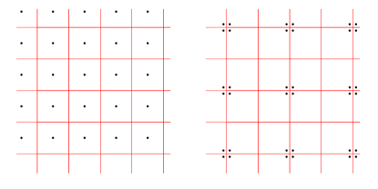
Figure 2: Two point distributions and their corresponding Voronoi tessellations. The important point illustrated by this example is that different point distributions may have identical Voronoi tessellations.

3.1 Viscous forces that help to improve order

Experience with our new VPH scheme shows that especially in highly irregular, turbulent flows and in situations with strong gravitational forces some cells can become quite irregular. In this context, we loosely define an irregular cell as one whose generating point is substantially displaced from the centroid of the cell and/or whose aspect ratio is quite high, i.e. a cell with a comparatively large ratio of surface area to volume. In this subsection we consider a scheme where the artificial viscosity is modified such that it serves a second purpose, namely to have the tendency to make cells ‘rounder’.

To this end we introduce the notion of a ‘partial pressure’ for each of the pyramids that make up a Voronoi cell. These pyramids are spanned by the Voronoi faces and the defining point of the cell, which acts as their apex. We define the ‘partial pressure’ of the pyramid of cell $i$ facing cell $j$ in terms of its volume $V_{ij}=A_{ij}R_{ij}/6$ (or $V_{ij}=A_{ij}R_{ij}/4$ in 2D) and by assigning a share $m_{ij}=m_{i}{A_{ij}}/{\sum_{k}A_{ik}}$ of the cell’s mass to the pyramid, i.e. its mass fraction is taken to be proportional to its contribution to the total surface area of the cell. This yields

$$P_{ij}=s_{i}\rho_{ij}^{\gamma}=s_{i}\left(\frac{6\,m_{i}}{R_{ij}\>\sum_{k}A_{ik}}\right)^{\gamma}.$$ (29)

The idea is now to define an additional viscous force between a pair of particles arising from the difference of this partial pressure to the full pressure of the cell. This will lead to rearrangements of the points until the differences in the partial pressures of each pyramid to that of the cell become small, which happens when the point is approximately equidistant to all the faces of its cell, implying a regular cell shape.

We hence make the ansatz

$$({\mn@boldsymbol{f}}_{\rm order})_{ij}=-\kappa A_{ij}(P_{ij}-P_{i}+P_{ji}-P_{j})\frac{{\mn@boldsymbol{e}}_{ij}}{2}$$ (30)

for ‘ordering forces’ between a pair of particles, with the total force on particle $i$ being given by

$$m_{i}({\mn@boldsymbol{a}}_{\rm order})_{i}=\sum_{j\neq i}({\mn@boldsymbol{f}}_{\rm order})_{ij}.$$ (31)

Here $\kappa$ is a dimensionless parameter describing the strength of the effect. These forces are antisymmetric, and in general can be both of repulsive and attractive nature. In order to maintain total energy conservation, the work of these forces needs to be balanced in the evolution of the entropies of the particles, similar to what is done for the ordinary artificial viscosity. This yields an additional contribution to the entropy change of the form

$$\frac{\mathrm{d}s_{i}}{\mathrm{d}t}=\frac{(\gamma-1)}{\rho_{i}^{\gamma-1}}\frac{1}{2}\sum_{j}({\mn@boldsymbol{f}}_{\rm order})_{ij}\cdot{\mn@boldsymbol{v}}_{ij}.$$ (32)

Note that a small local decrease of the entropy sum can result in principle if order is restored in the particle distribution, but this effect is small and has played no role in all our tests. In refinements of the above scheme, it is also possible to make $\kappa$ spatially and temporarily variable. For example, we have typically used this scheme in a combination with a switch that only sets $\kappa>0$ if there is a strong local compression, because that is where cell shapes distort the most.

When discussing results, we will refer to this method as ‘partial pressure ordering’ or PPO, whereas the method for improved cell regularity discussed in the next subsection will be referred to as ‘shape correction forces’. If none of these additional schemes to regularize cell shapes is employed, we simply refer to the method as the ‘plain Voronoi scheme’.

3.2 Imposing regularity through the fluid Lagrangian

If irregular cell shapes occur, we ideally would like that small adjustment forces appear naturally that tend to make the mesh more regular again. These adjustment forces should preserve the energy and momentum conservation of the scheme. This will automatically be the case if they are derived from a suitably defined Lagrangian or Hamiltonian. We are hence led to modify the fluid Lagrangian slightly to include factors that penalize highly distorted cell shapes. The idea is that such distorted cells should raise the estimate of the inner energy slightly, such that they become energetically disfavored.

We consider two ways to measure shape distortions of cells, which may either be used individually, or combined. One is based on the displacement of a point from the centroid of its associated cell. The idea here is that it is advantageous if a point stays close to the center of a cell. In particular, as we will discuss in more detail in Section 5.3, it turns out that the ordinary VPH scheme is not able to support waves in regular Cartesian grids at the Nyquist frequency, a deficit that could be cured if there is always a (weak) restoring force if a point is displaced from the centre of its Voronoi cell.

The other is to measure the shape directly, and to steer the particle motion such that high aspect ratios are avoided. We construct a shape measure based on the second moment of the cell, which we compare to a suitably defined cell radius. This measure will have a minimum for ‘round cells’, while severe distortions from roundness (like highly elongated cells) should trigger restoring forces.

Both of the above measures of cell regularity can be introduced into the fluid Lagrangian by multiplying the thermal energy with correction factors that increase the energy slightly if a point is displaced from the centroid, or if a cell is elongated. Specifically, we adopt as Lagrangian

$$L = \sum_{k}\frac{1}{2}m_{k}\dot{\mn@boldsymbol{r}}_{k}^{2}\quad-$$

$$\sum_{k}\frac{P_{k}V_{k}}{\gamma-1}\left[1+\beta_{0}\frac{({\mn@boldsymbol{r}}_{k}-{\mn@boldsymbol{s}}_{k})^{2}}{V_{k}^{2/d}}\right]\left\{1+\beta_{1}\left(\frac{{\mn@boldsymbol{w}}_{k}^{2}}{V_{k}^{2/d}}-\beta_{2}\right)\right\}.$$

Here ${\mn@boldsymbol{r}}_{k}$ is the coordinate of a point, $V_{k}$ is the volume of its corresponding Voronoi cell, and ${\mn@boldsymbol{s}}_{k}$ is the cell’s centroid. $P_{k}$ is the ordinary pressure of the cell, where we set $\rho_{k}=m_{k}/V_{k}$ as usual. The coefficients $\beta_{0}$ and $\beta_{1}$ are introduced to measure the strength of the correction forces associated with offsets from cell centres, or with high aspect ratios, respectively. For $\beta_{0}=\beta_{1}=0$, the ordinary fluid Lagrangian of the VPH scheme is recovered.

We define the centroid of a cell as

$${\mn@boldsymbol{s}}_{k}\equiv\left<{\mn@boldsymbol{r}}\right>_{k}=\frac{1}{V_{k}}\int{\mn@boldsymbol{r}}\,\chi_{k}({\mn@boldsymbol{r}})\,{\rm d}{\mn@boldsymbol{r}},$$ (34)

where $\chi_{k}$ is the characteristic function of cell $k$, i.e. $\chi_{k}({\mn@boldsymbol{r}})=1$ if the point ${\mn@boldsymbol{r}}$ lies in the cell $k$, and $\chi_{k}({\mn@boldsymbol{r}})=0$ otherwise. The shape of a cell is measured via the second moment

$${\mn@boldsymbol{w}}_{k}^{2}\equiv\left<({\mn@boldsymbol{r}}-{\mn@boldsymbol{s}}_{k})^{2}\right>_{k}=\frac{1}{V_{k}}\int({\mn@boldsymbol{r}}-{\mn@boldsymbol{s}}_{k})^{2}\chi_{k}({\mn@boldsymbol{r}})\,{\rm d}{\mn@boldsymbol{r}}.$$ (35)

The factors in squared and curly brackets in the Lagrangian of equation (3.2) are the adopted energy correction factors that raise the energy of distorted cells. Here $d$ counts the number of dimensions, i.e. $d=2$ for 2D and $d=3$ for 3D. The factor $V_{k}^{2/d}$ is hence proportional to the ‘radius’ $R_{k}=V_{k}^{1/d}$ of a cell squared. $\beta_{0}$ measures the strength of the effect of displacements of points from the centroid of a cell, while $\beta_{1}$ is the corresponding factor for the aspect-ratio factor. The constant $\beta_{2}$ is only introduced to prevent that even round cells lead to a significant enhancement of the thermal energy. For perfectly round cells, we expect in 2D approximately circles for which $w_{k}^{2}=V^{2/d}/(2\pi)$, hence we pick $\beta_{2}=1/(2\pi)$. In 3D, we have spherical shapes instead and we pick $\beta_{2}=3/5(3/4\pi)^{2/3}$.

The equations of motion for the Lagrangian (3.2) can be derived in closed form for the Voronoi mesh, but due to the length of the resulting expressions we give their derivation in Appendix B. The advantage of using the Lagrangian to obtain the cell-shaping forces is that the scheme then still accurately conserves total energy, momentum and entropy, while at the same time remaining translational and rotationally invariant. Also, the correction forces are ‘just right’ to achieve the desired regularity of the mesh, something that is difficult to achieve with any heuristic scheme to derive such forces, like the one we tried in the previous subsection.

In our results section, we show that this method is indeed capable of maintaining nicely regular meshes in the sense described above. However, we also caution that the stronger the extra forces are, the more unwanted features start to appear as well. First of all, the extra forces may introduce subtle deviations from the dispersion relation of an ideal gas, and may lead to spurious motions in situations with pressure equilibrium. The second, probably more serious side effect of this method may occur when the cells cannot easily relax to the desired regular cell structure, for example along a strong jump in density. In this case a pressure anomaly may develop due to the cell-shaping forces, similar to what is found in SPH across contact discontinuities. Still, we find that moderate values of $\beta_{0}$ and $\beta_{1}$ help to improve the accuracy of the VPH scheme without distorting the inviscid dynamics of an ideal gas too much.

4 Implementation

We have implemented the above hydrodynamical particle model into the cosmological TreeSPH simulation code GADGET-3, an updated version of GADGET-2 (Springel, 2005; Springel et al., 2001). This code is parallelized for distributed memory machines, and offers high-performance solvers for self-gravity as well as individual and adaptive timestepping for all particles. Our strategy in our modifications has been to implement Voronoi-based particle hydrodynamics as an alternative to SPH within the GADGET-3 code. This is, in particular, ideal for facilitating comparisons between SPH and our Voronoi-based scheme, and it also allows us to readily use all the non-standard physics already implemented in GADGET-3 (e.g. radiative cooling and star formation) for calculations with Voronoi-based fluid particle dynamics.

The primary new code needed in GADGET-3 is an efficient mesh construction algorithm. To this end we adapted and modified the parallel Delaunay triangulation engine from the AREPO code (Springel, 2009), and turned it into an optional module of the SPH code GADGET-3. In brief, the tessellation code uses an incremental construction algorithm for creating the Delaunay tessellation. Particles are inserted in turn into an already existing, valid tessellation. To this end, in a first step the tetrahedron in which the new point falls is located, and then it is split into several new tetrahedra, such that the inserted point becomes part of the tetrahedralization. However, some of the new tetrahedra may then not fulfill the empty-circumsphere property, i.e. the tessellation is not a Delaunay triangulation any more. Delaunayhood is restored in a second step by local flip operations that replace two adjacent tetrahedra with three tetrahedra, or vice versa, until all tetrahedra fulfill again the empty-circumsphere property. At this point, the next particle can be inserted. We have implemented the mesh construction both for 3D and 2D within the GADGET-3 code and parallelized it for distributed memory machines.

At the beginning, a large tetrahedron is constructed that encloses the full computational domain. The boundary conditions (always adopted as periodic at the moment) of the rectangular computational domain as well as the boundaries arising from the domain decomposition are treated with ‘ghost particles’. One technically difficult aspect is to make the tessellation code completely robust even in the case of the existence of degenerate particle distributions, where more than 4 points lie on a common circumsphere (or more than 3 points are on a common circumcircle). Detecting such a case robustly and correctly in light of the finite precision of floating point arithmetic is a non-trivial problem. However, the incremental insertion algorithm requires consistent and correct evaluations of all geometric predicates, otherwise it will typically fail in situations with degeneracies or near-degeneracies. We solve this problem by monitoring the floating point round-off in geometric tests, and by resorting to exact arithmetic in case there is a risk that the result of a geometric test may be modified by round-off error.

5 Test Results

In this section, we discuss a number of test problems carried out with our new hydrodynamical particle method, focusing in particular on regimes where differences with respect to SPH can be expected. An application of the method in full cosmological simulations of galaxy formation will be presented in future work.

5.1 Surface tension

In standard entropy-conserving SPH with particles, there is a subtle surface tension effect across contact discontinuities with a large jump in density. This can be understood as a result of the desire of SPH to suppress mixing of the two phases, because this is energetically unfavorable for fixed particle entropies. For the mixed state, approximately the same average density would be estimated for each particle, which leads to a higher estimate of the thermal energy, unless the thermodynamic entropies are averaged between the particles as well, which is an irreversible process in which entropy is in fact produced if the total energy stays constant.

To demonstrate the existence of the surface tension effect, we have prepared (in 2D for simplicity) an overdense ellipse in a thin background medium, at pressure equilibrium. For definiteness, the density of the ellipse was set to $\rho_{2}=4$, that of the background medium to $\rho_{1}=1$, with a pressure of $P=2.5$. 3854 equal mass particles in a periodic box of unit length on a side were used to set up the experiment. The particles have been arranged on a coarse Cartesian grid in which an ellipsoidal region was excised. This region has then be filled with a finer Cartesian grid. The specific entropies of the two sets of particles were initialized differently such that an equal pressure for the two phases results. No attempt was made to somehow soften the transition between the two phases. Figure 3 shows the initial configuration, as well as the particle distribution after a time $t=7$, both for SPH and for the Voronoi-based fluid particle approach.

Even though the pressures of the particles are formally equal for all particles in the initial conditions, the ellipse transforms to a circle when SPH is used. In contrast, for the VPH scheme, the same experiment maintains the initial shape of the ellipse, modulo some small rearrangements of the points near the boundary, since the initial set-up was not in perfect equilibrium (due to the fact that the point distributions of the two Cartesian grids used to set up the two phases do not match seamlessly at the boundary). Clearly, the numerical realization of the contact discontinuity in SPH gives rise to a spurious surface tension, and this in turn will suppress Kelvin-Helmholtz instabilities below a certain critical wavelength. The VPH approach does not have this problem and can in principle accurately support a contact discontinuity at each face boundary between individual cells. It needs to be stressed however that also in the Voronoi scheme no mixing of the entropies at the particle level happens. If the particles of two phases were simply spatially mixed while keeping their specific entropies constant, the resulting medium would not be at a single temperature or density. We note that the effect is also present for a set-up with unequal particle masses. In this case, the variationally derived entropy-conserving version of SPH will however lead to a change of the effective number of neighbours across the contact discontinuity, because it keeps the mass in the kernel volume constant.

Figure 3: Surface tension effect in SPH. The left column shows an overdense ellipsoidal region shortly after it is set-up at $t=0$ in pressure equilibrium within a thinner background. When evolved with SPH, the ellipsoid slowly transforms into a sphere, as shown by the state of the system after time $t=7$ (top left). In contrast, the Voronoi scheme can preserve the shape much better (bottom panels) and shows no sign of surface tension effects.

5.2 Sod shock tube

The classic Sod shock tube tests examine the ability of a hydrodynamic scheme to reproduce the basic wave structure that appears in the Riemann problem, namely shock waves, contact discontinuities and rarefaction waves. Also, comparison to the analytic solution gives a useful quantitative benchmark for the accuracy of a scheme.

We consider gas that is initially at rest. In the left half-space, the pressure is $P_{1}=1.0$ and the density is $\rho_{1}=1.0$, whereas in the right half-space we adopt $P_{2}=0.1795$ and $\rho_{2}=0.25$. The adiabatic index is set to $\gamma=1.4$. The same sod shock parameters have previously been used in a number of code tests (e.g. Hernquist & Katz, 1989; Rasio & Shapiro, 1991; Wadsley et al., 2004; Springel, 2005). When the evolution begins, a shock wave of Mach number $M=1.48$ travels into the low-pressure region, and a rarefaction fan moves into the high pressure region. In between, a moving contact discontinuity develops.

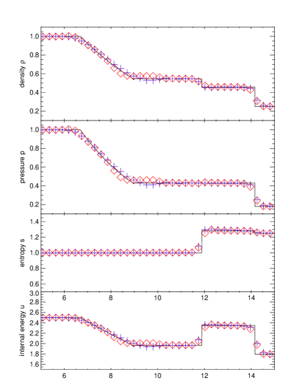
Figure 4: 3D Sod shock tube simulation at $t=3.0$. We compare results from our Voronoi particle scheme (blue crosses) and the SPH result with 32 neighbours (red diamonds) with the analytical solution (solid lines) in terms of the density, pressure, entropy profiles and internal energy.

In our numerical test of this problem with the VPH scheme we use a 3D setup in a box with dimensions $(20,1,1)$, where the left and right halves are filled with particles arranged on a Cartesian grid. Altogether 8370 particles with equal masses were used as initial condition. The evolution was then carried out with our default settings for the artificial viscosity until $t=3$. In Fig. 4, we compare the numerical result to the analytical solution at this time. Reassuringly, we find quite good agreement of the VPH scheme with the analytical solution. In comparison to SPH, the rarefaction wave in the Voronoi simulation shows a slight dip at the low density end, but not the hump at the high density end that is typical of SPH. Another difference is that the contact discontinuity is sharper and better preserved in the VPH approach. All of the described features appear to be largely independent of how the points are distributed initially as long as the gas is relaxed on both sides. In particular, the arrangement on a Cartesian grid does not lead to any noticeable artifacts compared with simulations where the initial point distribution is less ordered and has a glass-like configuration. However the results are somewhat less accurate for irregular grids (see also A.3) when the plain Voronoi scheme is used.

We have also examined the influence of the extra forces that can be enabled to improve the regularity of the mesh (see Sections 3.1 and 3.2). To this end we tested the effect of the PPO scheme as well as the shape correction method with parameters up to $\beta_{0}=1.2,\,\beta_{1}=0.1$. When these ordering forces are invoked, the results for the sod-shock test are in general not influenced much, but the particle noise around the analytical solution is reduced. We also found that the extent of postshock oscillations for weaker artificial viscosity settings tends to be reduced if these ordering methods are used.

5.3 Dispersion relations

Even though this may seem like a simple test, it is actually important to check how well our new method can simulate small-amplitude acoustic waves, especially at low resolution when few points per wavelength are available. We are especially interested in how accurately the expected dispersion relation is reproduced in this regime, i.e. whether such waves propagate with the correct speed of sound. A secondary question is how strongly such waves are damped by the artificial viscosity in the scheme.

To measure the dispersion relation, we set up small-amplitude standing waves in a periodic box and measure their oscillation frequency. In Figure 5, we compare results for SPH with our Voronoi-based fluid particle model, with and without shape correction forces, as a function of wavenumber. The wavenumber is normalized to the Nyquist frequency of the initial particle grid, such that $k/k_{\rm Nyquist}=1$ corresponds to the shortest wave that can be represented by the particles. In this standing wave, neighbouring particles oscillate 180 degrees out of phase ‘opposite’ to each other.

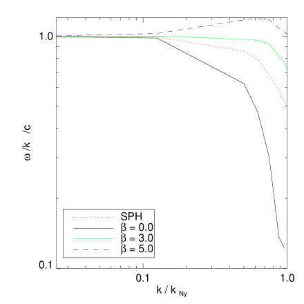
Figure 5: Dependence of the numerical sound speed on wavenumber, expressed in units of the Nyquist frequency of the underlying particle grid. For the standard VPH scheme, waves at the Nyquist frequency are not propagated properly (hence no frequency can be measured at $k=k_{\mathrm{Ny}}$), but this is remedied by the shape correction forces. If they are invoked, the resulting dispersion relation becomes more accurate than that of SPH for all $k$.

A first important result made clear by Figure 5 is that for the standard VPH scheme the oscillation frequency for $k/k_{\rm Nyquist}=1$ drops to zero, or in other words, such waves are not supported by the scheme at all. This is readily understood from the degeneracy effect pointed out in Figure 2. If particles are set-up such that they ‘collide’ in a pairwise fashion, then there is nothing in the reversible part of the dynamics of the VPH scheme that can prevent an interparticle penetration, simply because the pressure gradient stays zero in this case. However, this situation is exactly the one encountered if we prepare a standing wave at the Nyquist frequency of an initially regular particle grid. The wave will not oscillate since the pressure gradient will remain zero, and therefore particle crossings would be inevitable (unless prevented by the artificial viscosity). This is potentially a serious shortcoming of the VPH scheme in its standard form, as it means that it cannot treat waves at around the Nyquist frequency properly.

However, the shape correction force due to $\beta_{0}$ has exactly the right property to make these small waves oscillate again. In fact, we can calculate what value of $\beta_{0}$ is required to reproduce the dispersion relation at $k/k_{\rm Nyquist}=1$ exactly. For this value of $\beta_{0}\simeq 5.5$, we however also get slightly too stiff behaviour of the fluid for somewhat longer wavelengths, as shown by Fig. 5. A value of around $\beta_{0}\sim 3$ represents a good compromise, and in particular yields a more accurate dispersion relation than SPH for all $k$. We also note that for certain numbers of neighbours, the SPH result is inaccurate at all wavelength; here the numerical soundspeed shows an offset relative to the expected sound speed, which is presumably a result of a bias in the density estimate for the background density.

5.4 Density noise and regularity in a settled particle distribution

In this subsection we want to examine the level of noise present in a relaxed region of gas of constant specific entropy, as it may arise somewhere within a larger, self-consistent simulation. To mimic this situation, we start from a distribution of points arranged on a Cartesian grid and impose a random Gaussian velocity field with dispersion $\langle v^{2}\rangle=0.05\,c_{s}^{2}$ and zero mean. The idea is that these velocity fluctuations break the initial grid symmetry and will then get damped away by the artificial viscosity, which is here set to a high value to speed up the process of settling to a new pressure equilibrium. Since we want to retain the initially equal values of the specific entropies per particle, we disable the entropy source term for the viscosity in this experiment. Once the new equilibrium for an irregular particle distribution is achieved, we can then examine the noise properties of this particle representation of a constant density, constant pressure gas.

For SPH with $N=16$ neighbours, we find that the particles settle into several domains in which the points are quite regularly distributed, based on visual inspection. The estimated density values $\rho_{i}$ for the particles are not all equal though, instead they show a distribution with rms-scatter equal to $\sim 1.4\,\%$, and also a small bias relative to the expected value equal to the mean density $\left<\rho\right>=Nm/V$ of the full volume.

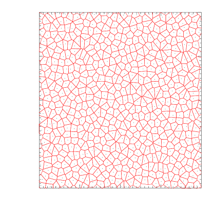
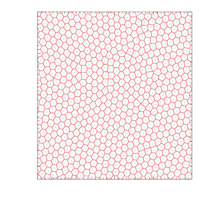
Figure 6: Final mesh geometry in VPH in a 2D settling test, carried out without (top) or with shape correction forces (bottom) based on $\beta_{0}=1.0$ and $\beta_{1}=0.01$.

In contrast, the standard VPH approach creates a distribution in which the density values are essentially single-valued, and are all very close to $\left<\rho\right>$. This means that the cells have all equal volume, and the residual pressure fluctuations, if any, are extremely small. However, the geometry of the Voronoi tessellation is quite irregular and features numerous cells with relatively large aspect ratios, or with points close to cell boundaries. This can be seen in Figure 6, where we show a plot of the final mesh for a test case carried out in 2D.

It is now interesting to repeat the test for the case when shape correction forces according to Section 3.2 are included. As desired, the final mesh becomes much more regular in this case, as seen in the corresponding example included in Figure 6. However, even in the final equilibrium state the correction forces do not necessarily completely vanish in this case. Instead, they are compensated by small residual pressure (and hence also density) fluctuations. This is demonstrated in the distribution functions of the density values for the three cases we considered, which we give in Figure 7. Here the shape correction case yields a somewhat broader distribution, similar to SPH, but without showing a bias.

In Figure 8, we give a quantitative measure for the cell-regularity (here taken as the distribution function of the normalized displacement of points from the centres of their cells) of the final meshes in the Voronoi-based simulations. Even moderate values of the coefficients $\beta_{0}$ and $\beta_{1}$ can drastically improve the regularity of the particle distribution while introducing less noise in the density estimate than anyway present in SPH.

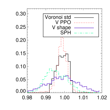
Figure 7: Density distribution functions of the particles in a settling test for constant entropy gas, carried out with different schemes. We compare SPH (red), ordinary VPH (black), the PPO version of VPH (blue), and VPH with shape correction forces based on $\beta_{0}=1.0$ and $\beta_{1}=0.01$ (in green). The distributions were measured at a time when the initial kinetic energy had decayed to $E_{\mathrm{kin}}\approx 0.001E_{\mathrm{kin}}(t=0)$.

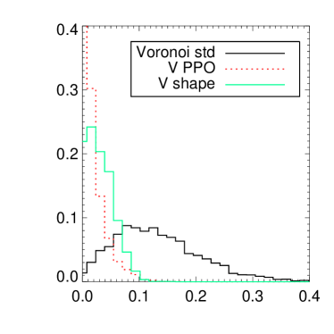
Figure 8: Cell-regularity of a noisy flow after relaxation. To characterize the regularity of the cells, we simply consider the distribution of the distance of the points to their cell’s centroids, in units of the 2D cell radius $r=\sqrt{{V}/{\pi}}$. The black histogram shows the distribution for the ordinary Voronoi scheme, blue shows the PPO version, and green lines give the result for the Voronoi with shape correction forces derived from the Lagrangian. The distributions were measured at a time when the initial kinetic energy had decayed to $E_{\mathrm{kin}}\approx 0.001E_{\mathrm{kin}}(t=0)$.

5.5 Point explosion

If energy is injected at a point into a cold gas at constant density, a spherical blast wave will develop. The Taylor-Sedov solution provides an analytic solution for this self-similar problem, which is a useful test involving very strong shocks. We have set-up this problem in 3D, using unit background density (represented with a Cartesian mesh), $\gamma=5/3$ and vanishingly small initial specific entropy compared to the injected energy of $E=1$. We inject the energy into the centre of the domain at time $t=0$. To avoid that the evolution is strongly affected by the non-spherical geometry of the central Voronoi cell, we have spread out the energy with a Gaussian kernel with a radius of about 4 mean particle spacings.

We note that this set-up can be especially sensitive to the problem of particle crossing when a too low viscosity and individual timesteps are used. In the latter case, the local Courant timestep of particles outside of the explosion is initially very big. When the supersonic shock front arrives, such particles may then still live on a too large timestep, such that they are effectively overtaken by the shock, creating severe artifacts in the evolution of the shock front. We have addressed this in our test by imposing a low enough maximum timestep for all particles, but more sophisticated schemes to set the timesteps, which guarantee that it is reduced before the shock arrives, can of course be implemented in principal (see Saitoh & Makino, 2009; Springel, 2009).

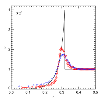
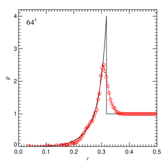
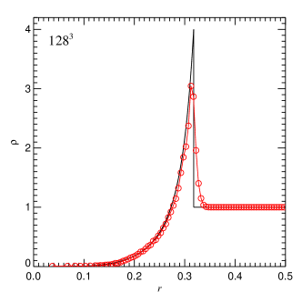
Figure 9: Sedov-Taylor point explosion problem, calculated in 3D with the basic VPH scheme. From top to bottom, we compare the radial density profile at $t=0.04$ with the analytical solution (solid line), calculated with $32^{3}$, $64^{3}$, or $128^{3}$ particles, as labeled. In the top panel, we also compare the VPH results (circles) with SPH (diamonds).

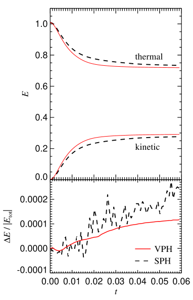
Figure 10: Time evolution of the thermal and kinetic energies in the Sedov-Taylor point explosion problem, simulated with SPH (black dashed line) and the Voronoi scheme with shape correction forces (red solid line). The bottom panel compares the total energy error in the two schemes.

In Figure 9, we show the radial density profile at $t=0.04$ for different resolutions corresponding to $2\times 32$, $2\times 64$ and $2\times 128$ particles, and compare to the expected analytic solution. The expected solution is captured reasonably well, with a similar quality as in SPH codes, which is shown for comparison in the low-resolution case. The VPH result converges nicely to the analytic solution as the resolution is increased. In particular, the shock location is well reproduced, albeit with a small pre-shock increase of the density. When shape correction forces are added as described in Section 3.2, only negligible differences in the overall quality of the result are found, but the scatter around the azimuthally averaged solution is reduced. In Figure 10, we check the energy conservation in the blast wave problem, both for the VPH and SPH simulations at the $32^{3}$ resolution. The energy error is negligibly small, as desired. The high-frequency oscillations in the total energy of the SPH run stem from the small but finite jumps of the SPH smoothing lengths from timestep to timestep, an effect that is absent in the VPH simulation.

5.6 Kelvin-Helmholtz instabilities

Kelvin-Helmholtz (KH) instabilities occur in regions of strong shear, which is especially common at contact discontinuities between two fluid phases. An initially small transverse perturbation along the interface becomes amplified and grows in linear theory according to $\propto\exp(t/t_{\rm KH})$. After a few characteristic timescales

$$t_{\rm KH}=\frac{\rho_{1}+\rho_{2}}{2\,k\,v\sqrt{\rho_{1}\rho_{2}}},$$ (36)

an initially wave-like perturbation becomes large and non-linear, developing the typical KH-rolls. Here $\rho_{1}$ and $\rho_{2}$ are the densities of the two media, $v$ is the velocity jump parallel to their common interface, and $k=2\pi/\lambda_{\rm pert}$ is the wavenumber of the perturbation with wavelength $\lambda_{\rm pert}$. For an ideal gas, all wavelengths are unstable, and the smallest wavelengths grow fastest.

The KH instability is especially important for the development of turbulence, and is thought to play a prominent role in stripping and mixing processes occurring during galaxy formation. Recently, a number of studies have pointed out that standard SPH has problems to correctly capture the KH instability when the initial conditions contain sharp density gradients (Agertz et al., 2007; Price, 2008). In certain cases, the instability is suppressed completely and does simply not grow. This can in part be understood in terms of the surface tension effect present in SPH, as described earlier, because surface tension suppresses the growth of KH instabilities below a critical wavelength (Landau & Lifshitz, 1966). Furthermore, the asymmetric particle density at the interface causes a rearrangement of the points in SPH, such that a ‘gap’ in the sampling appears that causes relatively large errors in the pressure forces at the interface (Agertz et al., 2007).

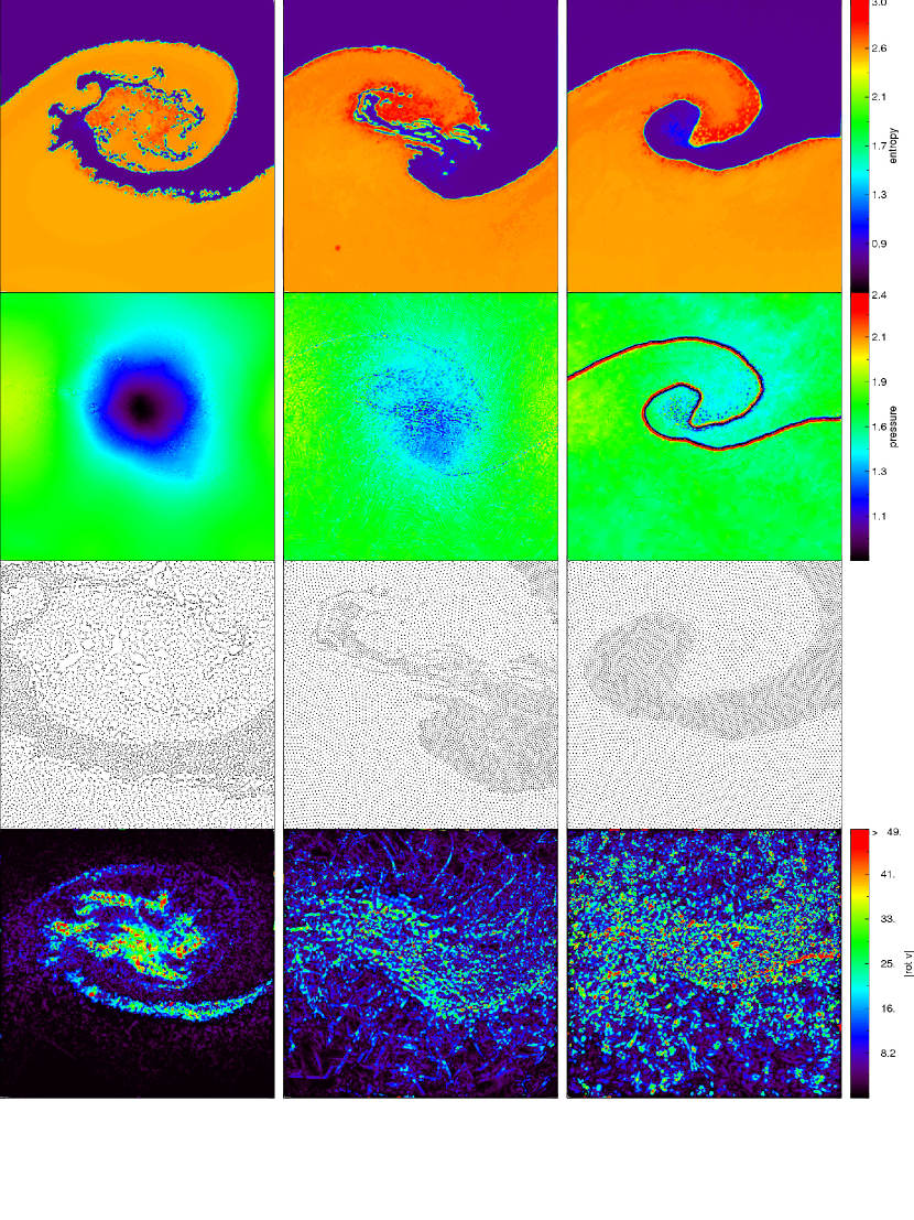
Figure 11: Simulations of the KH-instability with different particle-based methods. The left column shows the plain Voronoi scheme, the middle column Voronoi with PPO, and the right column SPH. From top to bottom, we show maps of specific entropy, maps of the pressure, the point distribution, and maps of the differential rotation $\nabla\times{\mn@boldsymbol{v}}$. The maps show $x=[0.18,0.58],y=[0,0.4]$ of the periodic simulation domain, while for clarity the particle distribution is shown only for $x=[0.28,0.48],y=[0.1,0.3]$.

It is therefore very interesting to test how well the VPH approach does in this respect. Since VPH does not exhibit a surface tension effect, it offers the prospect of a better treatment of the KH instability. In Figure 11, we show results for a KH test calculation, carried out with different particle-based hydrodynamic schemes. Our two-dimensional initial conditions consist of $\gamma=5/3$ gas with density $\rho_{1}=2$ in the stripe $|y-0.5|<0.25$, moving to the right with velocity $v_{1}=0.5$, and of gas with density $\rho_{2}=1$ and velocity $v_{2}=-0.5$ in the region $|y-0.5|\geq 0.25$. The pressure was initialized everywhere to $P=2.5$, and a periodic domain of unit length on a side was used. In total $261760$ points sample the gas distribution, with a mean spacing of $0.0023$ for the low-density gas, and $0.0017$ for the high density gas. Hence the two phases were represented with approximately equal mass particles. Note that the initial discontinuity was imposed as a perfectly sharp jump in these initial conditions, following previous studies of this problem. We remark however that it is somewhat questionable whether such sharp jumps are not introducing an inconsistency with the basic premises of SPH calculations, which can only represent smoothed density fields. In order to seed an initial perturbation, we imposed a vertical perturbation on the y-positions of the form

$$\delta y(x)=a_{0}\,\sin(4\pi x/L),$$ (37)

where $L$ is the boxsize, and $a_{0}=0.006$ is the amplitude of the initial perturbation.

The three columns of Figure 11 compare the results for the ordinary VPH scheme (left), the VPH method with the additional ordering viscosity of the PPO scheme (middle), and SPH (right), at time $t=1.2$. From top to bottom, we show specific entropy maps, pressure maps, the particle distribution, and vorticity maps. All maps were here generated by linearly interpolating a Delaunay tessellation of the points, allowing to extend the points’ properties as read from the simulation files to continuous fields. In addition to the maps, we show in Figure 12 the growth of the instability until time $t=1.2$, quantified in terms of the amplitude of the seeded velocity mode as measured in the Fourier-transformed $v_{y}$-field.

We see right away that the VPH scheme captures the KH instability best. Its primary KH billow has evolved furthest, and it triggered the growth of smaller-scale secondary billows. In contrast, the SPH result shows only an anemic growth of the instability. In the SPH pressure map a strong pressure anomaly is visible at the interface. This surface effect effectively suppresses all small-scale KH-instabilities, and the two phases stay separate because the associated surface tension suppresses a breaking up of the interface. As a result, the instability cannot cascade down to smaller scales. The PPO scheme shown in the middle column lies literally in the middle in this respect. The growth of the primary KH mode is very similar to that found in the VPH scheme. However, the additional viscosity introduced in this scheme to produce highly regular cells substantially attenuates the growth of secondary small-scale KH instabilities. The same effect can be seen Figure 12 for the case with shape correction terms, whereas additional heat diffusion (according to Section 2.5) does not affect the growth rate of the excited mode in this simulation. We note however that the smaller growth depends on the strength of the additional ordering forces that are invoked. The result shown here was calculated with $\kappa=1$, which we consider the maximum that one may ever want to use. For more reasonable smaller values, intermediate results that are close to that of the plain VPH scheme are obtained.

Interestingly, the vorticity $\nabla\times{\mn@boldsymbol{v}}$ in the ordinary VPH scheme is clearly largest overall, especially for the larger modes and in the central region of the primary KH billow. Here the rotation is so fast that the pressure shows a noticeable depression, which counteracts the centrifugal forces from the rotation with pressure gradients. Unfortunately, the ability of the pure Voronoi simulation to sustain vortices comes at the expense of a larger particle irregularity. As the enlargement with the particle distribution shows, the particles tend to form Voronoi cells with quite high aspect ratios, reducing the accuracy of the gradient estimates and requiring relatively large settings for the artificial viscosity to prevent interparticle penetrations. In contrast, the PPO variant of the Voronoi scheme produces highly regular particle spacings, and in this respect resembles SPH. However, in this example calculation with $\kappa=1$, the scheme then develops effectively a much higher intrinsic shear viscosity, which tends to transform the differential rotation into a rotation of numerous ordered domains. The shear of these domains shows up in the differential vorticity maps in a distribute fashion. Once the damping of the differential rotation gets too strong, the primary vortex is affected as well, as seen in the reduction of the central pressure gradient in the PPO scheme.

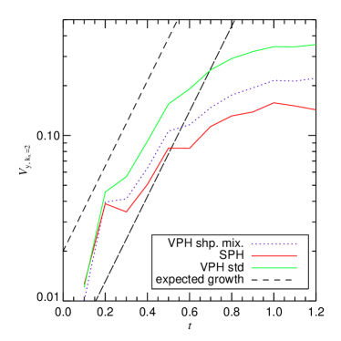
Figure 12: Growth rate of the KH-instability for the same initial conditions as in Figure 11. We show the amplitude of the seeded mode in the velocity field, measured by Fourier-transforming the $v_{y}$ field. We give results for standard VPH (green), for the Voronoi scheme with additional shape correction forces and the prescription for mixing discussed in Section 2.5 (dotted blue), and for SPH (red). The dashed black lines indicate the slope expected for an exponential growth of the instability according to linear theory.

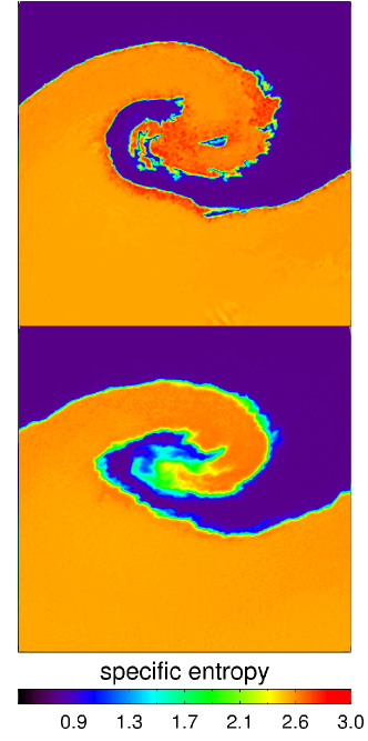
Figure 13: KH-instability test simulated with the Voronoi scheme with additional shape correction forces, based on the same initial conditions as in Figure 11 and again at time $t=1.2$. The maps show the entropy distribution without (top) and with (bottom) additional heat diffusion terms to model subresolution mixing, as described in Section 2.5.

Finally, we test the shape correction forces discussed in Section 3.2, and our scheme for the treatment of subresolution mixing introduced in Section 2.5 with the same initial conditions. We show in Fig. 13 the resulting entropy maps of two further calculations of the KH instability test. In both panels, we show runs of the VPH scheme that make use of the shape correction forces derived from the Lagrangian, with $\beta_{0}=1.2$ and $\beta_{1}=0.1$. In the bottom panel, we have in addition activated the artificial heat conduction due to local shear with $\chi=0.25$, which models mixing of the fluids at the scale of the resolution. The two variants are qualitatively similar, but the artificial heat conduction has clearly washed out the sharp discontinuity in the entropy at the fluid interface. This resembles more closely the results of mesh-based finite-volume hydro codes. Compared to the results of pure VPH in Figure 11, we see that the scheme with shape correction forces has also an effectively enlarged viscosity, quite similar to the PPO approach. Overall, it is clear that even without a subresolution mixing model the Voronoi based particle hydrodynamics does significantly better in the KH test than standard SPH.

5.7 The ‘blob test’: mass loss of a gas cloud in a supersonic wind

A challenging test problem for hydrodynamical codes has been proposed by Agertz et al. (2007). The setup consists of an overdense spherical cloud in pressure equilibrium with the surrounding hot medium. This background gas is given a large velocity, so that the cloud feels it as a supersonic head wind. The test is motivated by astrophysical situations such as the stripping of gas out of the halos of galaxies as they fall into larger systems. It is a three-dimensional problem that involves many different non-linear hydrodynamical phenomena, including shocks, Kelvin-Helmholtz instabilities, mixing, and the generation of turbulence. Because of this complexity, an analytical solution for the problem is not known. The general expectation is that the wind will compress the cloud, accelerate it, and strip some of its gas by developing fluid instabilities as it streams past the cloud.

Interestingly, in the test calculations of Agertz et al. (2007), substantial differences were found in the mass loss rates of the cloud when calculated with Eulerian mesh codes and with SPH. Whereas the mesh codes led to an eventual complete destruction of the cloud, the mass loss rate was in general smaller in SPH, such that some cloud material still remained once the partially destroyed cloud was accelerated to the wind speed and the mass loss stopped. Given these qualitatively different outcomes, it is interesting to test how the VPH scheme performs on this problem.

We used the same initial conditions as employed by Agertz et al. (2007), in the version with $10^{6}$ particles. The setup consists of a periodic box with extension $[0,2000]\times[0,2000]\times[0,8000]\,\mathrm{kpc}$. The background ‘wind’ gas has density $\rho_{\mathrm{wind}}=4.74\times 10^{-34}\,{\rm g\,cm^{-3}}$, temperature $T_{\rm wind}=10^{7}\,{\rm K}$, and a velocity $v_{\mathrm{wind}}=(0,0,1000)\,\mathrm{km\,s^{-1}}$. The cloud has a radius $R_{\mathrm{cloud}}=197\>\mathrm{kpc}$, and is placed initially at ${\mn@boldsymbol{r}}_{\mathrm{cloud}}=(1000,1000,1000)\,\mathrm{kpc}$. Its density is 10 times higher than the background, $\rho_{\mathrm{cloud}}=10\,\rho_{\mathrm{wind}}$, while at the same time being 10 times colder, $T_{\rm cloud}=10^{6}\,{\rm K}$. This yields a sound speed of $c_{\mathrm{wind}}=371\,\mathrm{km\,s^{-1}}$ for the wind, and an expected characteristic timescale of order $\tau_{\rm KH}\simeq 2\,{\rm Gyr}$ for the development of large KH instabilities in the shear-flow around the cloud.

In Figure 14, we show the time evolution of density slices through the central plane of the simulation box, calculated with our new Voronoi scheme. In agreement with both grid-based and SPH codes, a bow shock is produced ahead of the cloud. The cloud gets compressed and accelerated under the ram pressure of the wind, and the wind that streams past the deformed and slowly accelerating cloud induces Kelvin-Helmholtz instabilities at its surface which strip material and produce a turbulent wake. At the stagnation point of the flow in front of the cloud, the pressure eventually breaks through along the axis of symmetry. The resulting “smoke ring” is then still exposed to Kelvin-Helmholtz induced turbulence while it is being accelerated to the velocity of the background stream. Due to the periodic boundary conditions we note that the bow shock extends past the domain boundary and then back inwards again from the other side, reaching the cloud at about $t\approx 3\,\tau_{\rm KH}$. This leads to a recompression of the remainder of the cloud which can temporarily raise the number of particles that are still counted as cloud members.

The mass loss as a function of time is displayed in Figure 15, for different particle-based hydrodynamical schemes. We follow Agertz et al. (2007) and consider a particle to be still part of the cloud when its density is still larger than $\rho>0.64\>\rho_{\mathrm{cloud}}$, and its temperature fulfills $T<0.9\,T_{\mathrm{wind}}$. We show results for four different calculations in total. The standard VPH scheme is shown in blue. Interestingly, it leads to a complete destruction of the cloud at time $t\approx 3\,\tau_{\rm KH}$, a result which is actually surprisingly close to the high-resolution mesh-based calculations reported in Agertz et al. (2007). On the other hand, the two SPH-based results (shown in red and black) calculated with the GADGET2 code do not result in a destruction of the cloud. Instead at time $t=5\,\tau_{\rm KH}$, still about half the mass of the original cloud can be characterized as residual cloud material. This is even slightly larger than what was reported by Agertz et al. (2007) for the GASOLINE code. We have however found that the formulation and the strength of the artificial viscosity can influence this result significantly. Also, we confirmed that integration of the entropy as independent thermodynamic variable (which is the default in GADGET2) results in less stripped material than when the thermal energy is integrated as done in GASOLINE. This is however probably largely a result of the particular initial conditions used here; the contact discontinuity in the ICs of Agertz et al. (2007), that we employ here, has been relaxed using the traditional SPH formulation of GASOLINE, creating a pressure blip. When this is then used to initialize the entropies integrated in GADGET2, a spurious entropy blip is created that further amplifies the initial sampling ‘gap’.

When strong shape correction forces are introduced into the VPH formalism, we find an intermediate result between plain VPH and SPH. In this case, a small 10% remnant of the cloud remains at time $t=5\,\tau_{\rm KH}$. This is consistent with our earlier findings for the KH instabilities. While standard SPH can be expected to suppress the KH-instabilities significantly at the cloud interface, it tends to underestimate the rate of stripping. Our new VPH method does not show this problem, but if viscous forces are introduced that guarantee very regular mean particle separations, some small-scale suppression of fluid instabilities can be reintroduced.

We finally note that the use of a time variable viscosity as presently implemented in our code has not changed the mass-loss curves significantly. The reason is that the relevant particle viscosities are pushed to a large value as they pass through the bow shock, and stay at large values in the complicated flow around the cloud surface. Only at late times the mass loss tends to become faster as a result of the effectively lower viscosity.

Figure 14: Time evolution of the density for a gas cloud in a supersonic wind. From top to bottom, we show density maps normalized to the initial wind density at times $t=0.75\,\tau_{\mathrm{KH}}$, $t=1.5\,\tau_{\mathrm{KH}}$, and $t=2.25\tau_{\mathrm{KH}}$ in the central plane of the simulation box. Here the standard Voronoi scheme with $10^{6}$ particles was used.

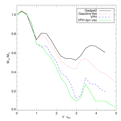
Figure 15: Mass loss of a gas cloud in a supersonic wind (the ‘blob test’), simulated with $10^{6}$ particles and different hydrodynamical schemes. We show the remaining mass associated with the cloud (particles that fulfill $\rho>0.64\>\rho_{\mathrm{cloud}}$ and $T<0.9\,T_{\mathrm{wind}}$) as a function of time (in units of $\tau_{\rm KH}$) for different hydrodynamical schemes. The different colors refer to the SPH codes GADGET2 (black), modified GADGET2 with an GASOLINE-like integration scheme (red), standard VPH (green), VPH with dynamic viscosity (see Equation 22 (light blue) and VPH with heat diffusion according to Section 2.5 (dark blue)

5.8 Gravitational collapse of a gas sphere

Finally, we consider a three-dimensional problem with self-gravity, the so-called ‘Evrard-collapse’ (Evrard, 1988). It consists of an initially cold gas cloud, with a spherically symmetric density profile of $\rho(r)\propto{1}/{r}$. The total mass, outer radius and gravitational constant are all set to unity, $M=R=G=1$, and the initial thermal energy per unit mass is set to $u=0.05$. In this configuration the sphere is significantly underpressurized. It hence collapses essentially in free-fall, until it bounces back at the centre, with a strong shock running through the infalling material. The sphere then settles into a new virial equilibrium. As this problem involves large conversions of potential gravitational energy into kinetic energy and thermal energy (and back), as well as strong shocks, it is a challenging and useful test for hydrodynamic codes that are applied to structure formation problems. For this reason, it has been widely used as a test for a number of SPH codes (e.g. Evrard, 1988; Hernquist & Katz, 1989; Steinmetz & Mueller, 1993; Dave et al., 1997; Springel et al., 2001; Wadsley et al., 2004; Springel, 2005).

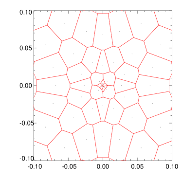
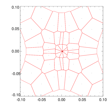
Figure 16: Cell regularity without (bottom) and with cell regularization forces (top) in a simulation of a sphere of gas collapsing under self-gravity (Evrard collapse problem). In the bottom panel, the group of points clusters together close to the origin under their mutual gravitational attraction, producing a quite irregular mesh there. This effect is prevented when additional shape correction forces are invoked, as shown in the top panel.

For our test we create a realization of the sphere by stretching a Cartesian grid appropriately, such that the desired initial density profile is obtained. Because the Voronoi scheme needs to tessellate a well-defined total volume, we cannot impose vacuum boundaries in the same way as in SPH. Instead, we embed the sphere in a box and use a background grid of particles with extremely rapidly falling density profile outside of the sphere, such that the total mass in the background can still be ignored in the evolution of the system. We calculate the gravity with the same tree algorithm used in the GADGET2 code, simply using the N-body approach with the masses and positions of the VPH particles. It turns out however that particles sometimes tend to pair up under their pairwise gravitational forces in the plain VPH scheme. This is related to the same defect discussed in the context of Figure 2. If two particles are very close to a Voronoi wall, they can be moved still closer together without increasing the hydrodynamic pressure force, so that a residual gravitational attraction (if not damped out by the gravitational softening) can move the particles very close together, with problematic consequences for the stability and accuracy of the scheme. A time-dependent gravitational softening (Price & Monaghan, 2007), where the softening is somehow tied to the size of the cell associated with a particle, may ease the problem, but is unlikely to cure it completely. However, the shape correction forces we introduced in Section 3.2 can nicely solve this problem. This effect is illustrated in Figure 16, where we show the central mesh geometry for a two-dimensional version of the Evrard collapse problem. In the following we consider therefore a calculation of the 3D Evrard collapse with our usual choice of $\beta_{0}=1.2$ and $\beta_{1}=0.1$.

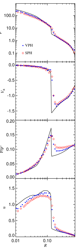
Figure 17: Evrard collapse at time $t=0.8$ simulated with SPH (red diamonds) and the Voronoi scheme with shape correction forces (blue circles). The black line shows the results of a 1D high-resolution PPM calculation of the problem provided to us by Steinmetz & Mueller (1993). From top to bottom, we show radially averaged profiles of gas density, radial gas velocity, specific entropy, and internal energy.

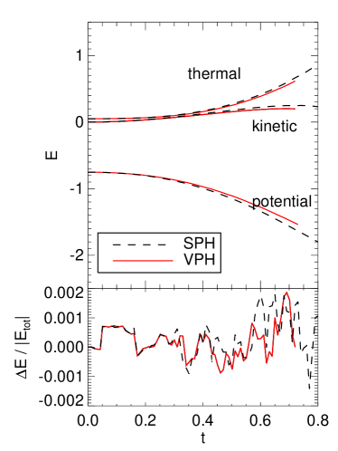
Figure 18: Energy evolution for the “Evrard collapse” simulated with SPH (black dashed line) and the Voronoi scheme with shape correction forces (red solid line). The small fluctuations in the total energy arise primarily as a result of the finite accuracy of the tree code used to calculate self-gravity, and are of similar magnitude for both cases.

In Figure 17, we show radial profiles of gas density, radial velocity and entropy for the Evrard collapse at time $t=0.8$, calculated with 24464 particles inside the initial sphere. We compare the VPH result (shown by blue circles) to results obtained with SPH (red diamonds), and compare these to results of a 1D high-resolution PPM calculation of the problem (solid black line) provided to us by Steinmetz & Mueller (1993). We find that the collapse is essentially equally well described with VPH as with SPH, with a slight advantage for VPH, which more accurately resolves the central density and captures the shock more sharply. However, these differences lie well in the range of changes one obtains for different viscosity prescriptions, and therefore do not seem to be particularly significant. We also note that the extra viscous forces needed to maintain a regular particle distribution in VPH do not introduce any unphysical features in the solution. In particular, the radial profile of the specific entropy shows no signs of extra cooling or heating.

6 Conclusions

We have discussed a new fluid particle model where the density is estimated with the Voronoi tessellation generated by the particle positions. Unlike in SPH, there is an auxiliary mesh, which adds complexity to the scheme. However, the use of this fully adaptive mesh offers a number of advantages. It offers higher resolution for a given number of particles, since fluid features are not inherently smoothed as in SPH. In fact, the tessellation techniques are probably close to an optimum exploitation of the density information contained in the particle distribution (Pelupessy et al., 2003). When even higher resolution is needed the method could be extended by an adaptive particle refinement or splitting technique, for example similar as suggested in (Springel, 2009).

As a result, contact discontinuities can be resolved with one cell, and surface tension effects present in standard SPH across contacts with large density jumps are eliminated. This has further implications for the growth rate of fluid instabilities in inviscid gases. Furthermore, the free parameters in the density estimate of SPH, involving both the number of neighbours as well as the kernel shape, are eliminated, which can be viewed as a good thing since the optimum values for them are not known, and incorrect choices can invoke the well-known clumping instability in SPH.

One somewhat problematic aspect of Voronoi-based particle hydrodynamics is that the noise in the scheme is quite sensitive to the level of mesh regularity. Flows with a lot of shear can readily develop Voronoi meshes with points that lie close to the surfaces of their Voronoi cells. In this case the noise in the gradient estimates increases, and, more importantly, it becomes difficult to safely prevent particle interpenetration, since closeness to a wall of the tessellation always implies that there is a second point on the other side of the wall which is also close, i.e. in other words, that a close particle pair is present.

Higher order density estimates might solve this problem, but they would have to be introduced already into the Lagrangian, leading to much more complicated equations of motion that may be intractable. We therefore explored two different approaches for keeping the mesh relatively regular. One is simply based on trying to formulate additional artificial viscosity terms such that the viscosity tries to make cells ‘rounder’. Whereas this shows some success, it does not succeed in all situations, particularly in strong shear flows where the artificial viscosity needs to be very low. A more radical approach also explored is to add correction terms to the underlying fluid Lagrangian with the aim to penalize strong deviations from regular mesh geometries. Our goal was to impose small, non-dissipative correction forces that maintain a proper mesh geometry. Thanks to the Lagrangian formulation, the required form of the correction forces to retain fully conservative behaviour can readily be derived, and the fluid motion under these forces shows the desired properties. However, if the correction terms are too large, one risks deviations from the proper hydrodynamic solution. Further experimentation will be required to identify the optimum setting of these parameters.

The Voronoi-based fluid particle approach can be relatively seamlessly integrated into an existing SPH code, provided a tessellation engine can be added in an appropriate fashion. Other aspects of the physics (in particular self-gravity, an additional collisionless component, radiative cooling, star formation, and feedback processes) can be treated in essentially identical ways as in SPH. This makes it possible to readily apply Voronoi particle hydrodynamics to problems of interest in cosmological structure formation. In general, our first results suggest that VPH is superior to SPH, albeit at much increased complexity. However, it is at present still unclear whether it is competitive with finite volume hydrodynamics carried out on a similarly constructed Voronoi mesh, as realized in the AREPO code (Springel, 2009). To elucidate this point further, we are in the process of carrying out galaxy collision simulations as well as cosmological structure formation simulations with our new technique and will report the results in forthcoming work.

Appendix A Differential operators on Voronoi meshes

In this Appendix, we collect some useful formulae for discretized versions of differential operators on Voronoi meshes, such as the gradient or the divergence, and we test the accuracy of the gradient estimate as a function of the regularity of the Voronoi mesh.

A.1 Gradient

The cell averaged gradient of any quantity $\phi$ can be estimated via Gauss’ theorem. One can use Gauss’ theorem on a product of a constant vector times a scalar field and arrives at:

$$\frac{1}{V}\int_{V}{\mn@boldsymbol{\nabla}}\phi\>{\rm d}V=\frac{1}{V}\int_{\partial V}\phi\>{\rm d}{\mn@boldsymbol{S}},$$ (38)

which can be used as one way to derive an estimate of the local gradient by approximating the value of $\phi$ on the surface of a cell with the arithmetic mean between the cell and its neighbours. However, one can also circumvent the problem of finding a proper value for $\phi$ on the surface by using a different starting point. We now use Gauss’ theorem on $({\mn@boldsymbol{1}}\cdot{\mn@boldsymbol{r}})\,{\mn@boldsymbol{\nabla}}\phi$, where ${\mn@boldsymbol{1}}$ is the unit vector. This yields:

$$\int_{V}{\mn@boldsymbol{\nabla}}\phi{\rm d}V=\int_{\partial V}{\mn@boldsymbol{r}}({\mn@boldsymbol{\nabla}}\phi\cdot{\rm d}{\mn@boldsymbol{S}})-\int_{V}{\mn@boldsymbol{r}}\Delta\phi{\rm d}V$$ (39)

With the help of $R_{ij}=|{\mn@boldsymbol{r}}_{j}-{\mn@boldsymbol{r}}_{i}|$ as the distance between points $i$ and $j$, and ${\mn@boldsymbol{r}}^{\perp}$ as ${\mn@boldsymbol{r}}$ projected onto the plane of the face $A_{ij}$ (for definition see Fig. 1 and Fig 19),

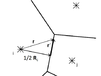
Figure 19: Sketch of the integration variables

${\mn@boldsymbol{r}}$ becomes ${\mn@boldsymbol{r}}={\mn@boldsymbol{r}}^{\perp}+({\mn@boldsymbol{r}}_{i}-{\mn@boldsymbol{r}}_{j})/2+{\mn@boldsymbol{r}}_{i}$, and then the right hand side can be discretized for the Voronoi mesh as follows:

$$\int_{\partial V}{\mn@boldsymbol{r}}({\mn@boldsymbol{\nabla}}\phi\cdot{\rm d}{\mn@boldsymbol{S}}) = \sum_{j\neq i}\int_{A_{ij}}{\mn@boldsymbol{r}}({\mn@boldsymbol{\nabla}}\phi\cdot{\rm d}{\mn@boldsymbol{S}})\quad\quad-\int_{V_{i}}{\mn@boldsymbol{r}}\Delta\phi{\rm d}V$$ (40)

$$= \sum_{j\neq i}\int_{A_{ij}}\left(\frac{1}{2}{\mn@boldsymbol{R}}_{ij}+{\mn@boldsymbol{r}}^{\perp}\right)({\mn@boldsymbol{\nabla}}\phi\cdot{\mn@boldsymbol{e}}_{ij}){\rm d}S\quad+{\mn@boldsymbol{r}}_{i}\sum_{j\neq i}\int_{A_{ij}}({\mn@boldsymbol{\nabla}}\phi\cdot{\mn@boldsymbol{e}}_{ij}){\rm d}S\quad\quad-\int_{V_{i}}{\mn@boldsymbol{r}}\Delta\phi{\rm d}V$$ (41)

$$= \sum_{j\neq i}({\mn@boldsymbol{\nabla}}\phi\cdot{\mn@boldsymbol{R}}_{ij})A_{ij}\left(\frac{1}{2}{\mn@boldsymbol{e}}_{ij}+\frac{1}{R_{ij}A_{ij}}\int_{A_{ij}}{\mn@boldsymbol{r}}^{\perp}{\rm d}S\right)\quad+{\mn@boldsymbol{r}}_{i}\int_{V_{i}}\Delta\phi{\rm d}V\quad\quad-\int_{V_{i}}{\mn@boldsymbol{r}}\Delta\phi{\rm d}V$$ (42)

$$= \sum_{j\neq i}({\mn@boldsymbol{\nabla}}\phi\cdot{\mn@boldsymbol{R}}_{ij})A_{ij}\left(\frac{1}{2}{\mn@boldsymbol{e}}_{ij}+\frac{{\mn@boldsymbol{c}}_{ij}}{R_{ij}}\right)\quad\quad-\quad\quad\int_{V_{i}}\left({\mn@boldsymbol{r}}-{\mn@boldsymbol{r}}_{i}\right)\Delta\phi{\rm d}V$$ (43)

The second term vanishes for linear scalar fields. It is therefore only a second order correction that becomes negligible for sufficiently smooth fields if the points lie near the centroids of their cells so that $\int_{V}\left({\mn@boldsymbol{r}}-{\mn@boldsymbol{r}}_{i}\right){\rm d}V$ .
Now we use ${\mn@boldsymbol{R}}_{ij}\cdot{\mn@boldsymbol{\nabla}}\phi=(\phi_{j}-\phi_{i})$, so that we obtain for the gradient estimate $\left({\mn@boldsymbol{\nabla}}\phi\right)_{i}$ at point $i$

$$\left({\mn@boldsymbol{\nabla}}\phi\right)_{i} = \frac{1}{V_{i}}\sum_{j\neq i}(\phi_{j}-\phi_{i})A_{ij}\left(\frac{1}{2}{\mn@boldsymbol{e}}_{ij}+\frac{{\mn@boldsymbol{c}}_{ij}}{R_{ij}}\right)$$ (45)

$$= \frac{1}{V_{i}}\sum_{j\neq i}A_{ij}\left[(\phi_{j}-\phi_{i})\frac{{\mn@boldsymbol{c}}_{ij}}{R_{ij}}+(\phi_{j}+\phi_{i})\frac{{\mn@boldsymbol{e}}_{ij}}{2}\right].$$ (46)

We note that application of this gradient estimate to the Euler momentum equation in the form

$$m_{i}\ddot{\mn@boldsymbol{r}}_{i}=-V_{i}\,{\mn@boldsymbol{\nabla}}P_{i}$$ (47)

yields

$$m_{i}\ddot{\mn@boldsymbol{r}}_{i}=-\sum_{j\neq i}A_{ij}\left[(P_{j}-P_{i})\frac{{\mn@boldsymbol{c}}_{ij}}{R_{ij}}\>+\>(P_{j}+P_{i})\>\frac{{\mn@boldsymbol{e}}_{ij}}{2}\right]$$ (48)

which is consistent with the expression derived directly from the Lagrangian.

A.2 Divergence and curl

To estimate the divergence and curl of the velocity which we need for the viscosity calculation of Section 2.4 we use the same reasoning as in 39.

$$\int_{V_{i}}\left({\mn@boldsymbol{r}}\nabla\left(\nabla{\mn@boldsymbol{v}}\right)\>+\>\nabla{\mn@boldsymbol{v}}\right){\rm d}V=\int_{\partial V}{\mn@boldsymbol{r}}(\nabla{\mn@boldsymbol{v}}\cdot{\rm d}{\mn@boldsymbol{S}}).$$ (49)

Provided that $\frac{1}{V_{i}}\int_{V_{i}}\nabla\times\left(\nabla\times{\mn@boldsymbol{v}}\right)$ vanishes for a linear field we define our estimator for the divergence operator as

$$(\nabla\cdot{\mn@boldsymbol{v}})_{i}=-\frac{1}{V_{i}}\sum_{j\neq i}A_{ij}\left[({\mn@boldsymbol{v}_{j}}-{\mn@boldsymbol{v}_{i}})\cdot\left(\frac{1}{2}{\mn@boldsymbol{e}}_{ij}+\frac{{\mn@boldsymbol{c}}_{ij}}{R_{ij}}\right)\right].$$ (50)

Similarly, the curl estimator can be defined in the form

$$(\nabla\times{\mn@boldsymbol{B}})_{i}=-\frac{1}{V_{i}}\sum_{j\neq i}A_{ij}\left[({\mn@boldsymbol{B}_{j}}-{\mn@boldsymbol{B}_{i}})\times\left(\frac{1}{2}{\mn@boldsymbol{e}}_{ij}+\frac{{\mn@boldsymbol{c}}_{ij}}{R_{ij}}\right)\right],$$ (51)

where ${\mn@boldsymbol{B}}$ denotes some vector field. Again applying Gauss’ theorem to $\nabla\phi$ the Laplacian of a scalar function $\phi$ can be computed as

$$\int_{V}\Delta\phi\>{\rm d}V=\sum_{j\neq i}\int_{A_{ij}}({\mn@boldsymbol{\nabla}}\phi\cdot{\rm d}{\mn@boldsymbol{S}})\simeq\sum_{j\neq i}A_{ij}\frac{\phi_{j}-\phi_{i}}{R_{ij}}.$$ (52)

A.3 Accuracy of the gradient

To test the accuracy of the numerical gradient estimate, we assume a quadratic model function $\phi({\mn@boldsymbol{r}})$ with constant gradient and Hesse matrix, of the form

$$\phi({\mn@boldsymbol{r}})=\phi_{0}+{\mn@boldsymbol{A}}{\mn@boldsymbol{r}}+\frac{1}{2}{\mn@boldsymbol{r}}^{T}{\mn@boldsymbol{B}}{\mn@boldsymbol{r}}.$$ (53)

For definiteness, we set ${\mn@boldsymbol{B}}=b{\mn@boldsymbol{I}}$, where ${\mn@boldsymbol{I}}$ is the identity matrix. We then populate a box of unit length on a side with a set of points, and evaluate the function $\phi({\mn@boldsymbol{r}})$ at the coordinates of each of the points. After constructing the Voronoi tessellation for the point set, we then estimate the local gradient for each cell based on

$$(\nabla\phi)_{i}=\frac{1}{V_{i}}\sum_{j}(\phi_{j}-\phi_{i})\>A_{ij}\left(\frac{1}{2}{\mn@boldsymbol{e}}_{ij}+\frac{{\mn@boldsymbol{c}}_{ij}}{R_{ij}}\right),$$ (54)

and alternatively also based on a simpler version of this formula where the terms proportional to ${\mn@boldsymbol{c}}_{ij}$ are omitted, which corresponds to the simplest version of a Green-Gauss gradient estimate. We use three different point distributions with $4096$ points in a box of size unity. First we use a (i) random Poisson point distribution, a (ii) relaxed point distribution obtained from the VPH scheme where each cell has the same volume (obtained from the top of Fig. 6), and (iii) a distribution relaxed with PPO (obtained from the bottom of Fig. 6) where in addition very round cells were produced in which the majority of the points lies close to the geometric centres of the cells. In all three cases we compare the magnitude of the estimated gradient vector to the magnitude of ${\mn@boldsymbol{A}}$, and we plot the median of the relative error as a function of $b/|{\mn@boldsymbol{A}}|$. To exclude boundary effects, only cells whose neighbours do not overlap with the box boundary are considered in the measurement.

In Figure 20, we show the results. The panel on the left gives our adopted gradient estimate, while the panel on the right is for the simpler version of the Green-Gauss gradient estimate. Interestingly, for $b=0$, the error vanishes exactly, independent of the regularity of the Voronoi mesh. However, once the second order term starts to influence the measurement, i.e. for large values if $b/|{\mn@boldsymbol{A}}|$, the more regular meshes clearly yield a lower error, as expected. In all cases, the gradient estimate that includes the ${\mn@boldsymbol{c}}_{ij}$ term is superior to the simple Green-Gauss gradient estimate. In particular, only when it is included, a vanishing error for a linearly varying field is obtained.

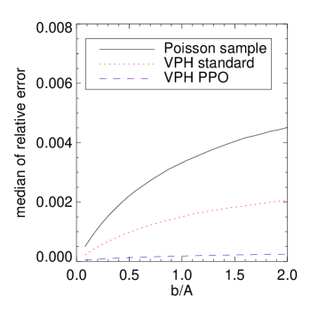
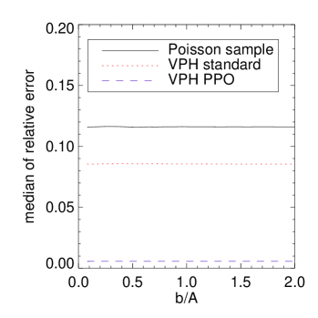
Figure 20: Median relative error in the gradient estimate obtained either with our default formula (left) or with the simpler Green-Gauss estimate where the ${\mn@boldsymbol{c}}_{ij}$ terms are omitted (right). We show results for three different types of point sets, a Poisson sample (black), a regularized distribution where each Voronoi cell has equal volume (red), and a regularized distribution where in addition the cells are quite ‘round’ and regular (blue). The accuracy is measured as function of the strength of a second order variation in the underlying field.

Appendix B Controlling the shape of cells

As outlined in Section 3.2, we modify the fluid Lagrangian slightly to include factors that penalize highly distorted cell shapes. If such shapes occur, we want small adjustment forces to appear that tend to make the mesh more regular again. These adjustment forces need to preserve energy and momentum conservation of the scheme, which will automatically be the case if they are derived from a suitably defined Lagrangian or Hamiltonian. In this Appendix, we derive the equations of motion for the Lagrangian

$$L=\sum_{k}\frac{1}{2}m_{k}\dot{\mn@boldsymbol{r}}_{k}^{2}-\sum_{k}\frac{P_{k}V_{k}}{\gamma-1}\left[1+\beta_{0}\frac{({\mn@boldsymbol{r}}_{k}-{\mn@boldsymbol{s}}_{k})^{2}}{V_{k}^{2/d}}\right]\left\{1+\beta_{1}\left(\frac{{\mn@boldsymbol{w}}_{k}^{2}}{V_{k}^{2/d}}-\beta_{2}\right)\right\},$$ (55)

where the factor in square brackets disfavours displacements of points from the geometric centres of their cells, and the factor in curly brackets disfavours cells with large aspect ratios.

We define the centroid of a cell as

$${\mn@boldsymbol{s}}_{k}\equiv\left<{\mn@boldsymbol{r}}\right>_{k}=\frac{1}{V_{k}}\int{\mn@boldsymbol{r}}\,\chi_{k}({\mn@boldsymbol{r}})\,{\rm d}{\mn@boldsymbol{r}},$$ (56)

where $\chi_{k}$ is the characteristic function of cell $k$. The shape of a cell is measured via the second moment

$${\mn@boldsymbol{w}}_{k}^{2}\equiv\left<({\mn@boldsymbol{r}}-{\mn@boldsymbol{s}}_{k})^{2}\right>_{k}=\frac{1}{V_{k}}\int({\mn@boldsymbol{r}}-{\mn@boldsymbol{s}}_{k})^{2}\chi_{k}({\mn@boldsymbol{r}})\,{\rm d}{\mn@boldsymbol{r}}.$$ (57)

Here $d$ counts the number of dimensions, i.e. $d=2$ for 2D and $d=3$ for 3D. The factor $V_{k}^{2/d}$ is hence proportional to the ‘radius’ $R_{k}=V_{k}^{1/d}$ of a cell squared. $\beta_{0}$ measures the strength of the effect of displacements of points from the centroid of a cell, while $\beta_{1}$ is the corresponding factor for the aspect-ratio factor. The constant $\beta_{2}$ is only introduced to prevent that even round cells lead to a significant enhancement of the thermal energy. For perfectly round cells, we expect in 2D roughly circles for which $w_{k}^{2}=V^{2/d}/(2\pi)$, hence we pick $\beta_{2}=1/(2\pi)$. In 3D, we have approximately spheres instead and we pick $\beta_{2}=3/5(3/4\pi)^{2/3}$.

Note that this Lagrangian is only a function of the point coordinates for given entropies, so the equations of motion for conservative dynamics are perfectly well defined, even though they lead to more lengthy expressions than in the standard case. We first obtain the following Lagrangian equation of motion:

$$m_{i}\ddot{\mn@boldsymbol{r}}_{i}=\frac{\partial L}{\partial{\mn@boldsymbol{r}}_{i}}=-\sum_{k}\frac{1}{\gamma-1}\left(\frac{\partial}{\partial{\mn@boldsymbol{r}}_{i}}P_{k}V_{k}\right)\Big{[}\,\Big{]}\Big{\{}\,\Big{\}}\;-\;\sum_{k}\frac{P_{k}V_{k}}{\gamma-1}\Big{\{}\,\Big{\}}\beta_{0}\frac{\partial}{\partial{\mn@boldsymbol{r}}_{i}}\frac{({\mn@boldsymbol{r}}_{k}-{\mn@boldsymbol{s}}_{k})^{2}}{V_{k}^{2/d}}\;-\;\sum_{k}\frac{P_{k}V_{k}}{\gamma-1}\Big{[}\,\Big{]}\beta_{1}\frac{\partial}{\partial{\mn@boldsymbol{r}}_{i}}\frac{w_{k}^{2}}{V_{k}^{2/d}},$$ (58)

where the empty square and curly brackets are notational short-cuts for the corresponding terms in the original Lagrangian. We note that we can use the identity

$$\frac{\partial}{\partial{\mn@boldsymbol{r}}_{i}}P_{k}V_{k}=(1-\gamma)P_{k}\frac{\partial V_{k}}{\partial{\mn@boldsymbol{r}}_{i}}.$$ (59)

We also note that in the second and third terms of equation (58) we encounter partial derivatives of $V_{k}$, which we can combine with the first term into a more compact form. This allows us to write the equation of motion in the form

$$m_{i}\ddot{\mn@boldsymbol{r}}_{i}=\sum_{k}P_{k}^{\star}\frac{\partial V_{k}}{\partial{\mn@boldsymbol{r}}_{i}}\;-\;\sum_{k}Q_{k}\frac{\partial}{\partial{\mn@boldsymbol{r}}_{i}}({\mn@boldsymbol{r}}_{k}-{\mn@boldsymbol{s}}_{k})^{2}\;-\;\sum_{k}L_{k}\frac{\partial}{\partial{\mn@boldsymbol{r}}_{i}}w_{k}^{2}$$ (60)

where we have defined

$$P_{k}^{\star}\equiv P_{k}\left(\Big{[}\,\Big{]}\Big{\{}\,\Big{\}}+\frac{2}{d}\frac{\beta_{0}}{\gamma-1}\frac{({\mn@boldsymbol{r}}_{k}-{\mn@boldsymbol{s}}_{k})^{2}}{V_{k}^{2/d}}\Big{\{}\,\Big{\}}+\frac{2}{d}\frac{\beta_{1}}{\gamma-1}\frac{w_{k}^{2}}{V_{k}^{2/d}}\Big{[}\,\Big{]}\right)$$ (61)

and introduced the quantities

$$Q_{k}\equiv\frac{\beta_{0}}{\gamma-1}P_{k}V_{k}^{1-2/d}\Big{\{}\,\Big{\}},$$ (62)

$$L_{k}\equiv\frac{\beta_{1}}{\gamma-1}P_{k}V_{k}^{1-2/d}\Big{[}\,\Big{]}.$$ (63)

We already know an explicit expression for ${\partial V_{k}}/{\partial{\mn@boldsymbol{r}}_{i}}$, but we still need to derive such a thing for the derivatives of $({\mn@boldsymbol{r}}_{k}-{\mn@boldsymbol{s}}_{k})^{2}$ and $w_{k}^{2}$. Let us first deal with the term involving $Q_{k}$ in the equations of motion, i.e.

$$\left(m_{i}\ddot{\mn@boldsymbol{r}}_{i}\right)_{Q}=-\sum_{k}Q_{k}\frac{\partial}{\partial{\mn@boldsymbol{r}}_{i}}({\mn@boldsymbol{r}}_{k}-{\mn@boldsymbol{s}}_{k})^{2}=-2\sum_{k}Q_{k}\left(\frac{\partial({\mn@boldsymbol{r}}_{k}-{\mn@boldsymbol{s}}_{k})}{\partial{\mn@boldsymbol{r}}_{i}}\right)^{T}({\mn@boldsymbol{r}}_{k}-{\mn@boldsymbol{s}}_{k}).$$ (64)

Here the exponent $T$ stands for the transpose, and the notation $\frac{\partial{\mn@boldsymbol{a}}}{\partial{\mn@boldsymbol{b}}}$ is the Jacobian matrix with elements $\left(\frac{\partial{\mn@boldsymbol{a}}}{\partial{\mn@boldsymbol{b}}}\right)_{lm}=\frac{\partial a_{l}}{\partial b_{m}}$. Based on the definition of ${\mn@boldsymbol{s}}_{k}$ in terms of the characteristic function we find

$$\frac{\partial}{\partial{\mn@boldsymbol{r}}_{i}}({\mn@boldsymbol{r}}_{k}-{\mn@boldsymbol{s}}_{k})=\delta_{ki}\mathbf{1}-\frac{1}{V_{k}}({\mn@boldsymbol{r}}_{k}-{\mn@boldsymbol{s}}_{k})\left(\frac{\partial V_{k}}{\partial{\mn@boldsymbol{r}}_{i}}\right)^{T}+\frac{1}{V_{k}}\int{\rm d}{\mn@boldsymbol{r}}\,({\mn@boldsymbol{r}}_{k}-{\mn@boldsymbol{r}})\left(\frac{\partial\chi_{k}}{\partial{\mn@boldsymbol{r}}_{i}}\right)^{T}.$$ (65)

For the derivative of the characteristic function we can use a result from Serrano & Español (2001) and write

$$\frac{\partial\chi_{k}}{\partial{\mn@boldsymbol{r}}_{i}}=\sum_{j}\delta_{ki}\frac{\chi_{k}\chi_{j}}{\sigma^{2}}\,({\mn@boldsymbol{r}}-{\mn@boldsymbol{r}}_{k})-\frac{\chi_{k}\chi_{i}}{\sigma^{2}}\,({\mn@boldsymbol{r}}-{\mn@boldsymbol{r}}_{i}),$$ (66)

which is based on approximating the characteristic function with

$$\chi_{k}({\mn@boldsymbol{r}})=\frac{\exp\left[-\frac{({\mn@boldsymbol{r}}-{\mn@boldsymbol{r}}_{k})^{2}}{2\sigma^{2}}\right]}{\sum_{j}\exp\left[-\frac{({\mn@boldsymbol{r}}-{\mn@boldsymbol{r}}_{j})^{2}}{2\sigma^{2}}\right]},$$ (67)

which becomes exact in the limit $\sigma\to 0$. Putting these results into equation (64) one gets

$$\left(m_{i}\ddot{\mn@boldsymbol{r}}_{i}\right)_{Q} = -2Q_{i}({\mn@boldsymbol{r}}_{i}-{\mn@boldsymbol{s}}_{i})+2\sum_{k}\frac{Q_{k}}{V_{k}}({\mn@boldsymbol{r}}_{k}-{\mn@boldsymbol{s}}_{k})^{2}\frac{\partial V_{k}}{\partial{\mn@boldsymbol{r}}_{i}}-2\sum_{j}\frac{Q_{i}}{V_{i}}\int{\rm d}{\mn@boldsymbol{r}}\frac{\chi_{i}\chi_{j}}{\sigma^{2}}({\mn@boldsymbol{r}}-{\mn@boldsymbol{r}}_{i})({\mn@boldsymbol{r}}_{i}-{\mn@boldsymbol{r}})^{T}({\mn@boldsymbol{r}}_{i}-{\mn@boldsymbol{s}}_{i})$$ (68)

$$+2\sum_{k}\frac{Q_{k}}{V_{k}}\int{\rm d}{\mn@boldsymbol{r}}\frac{\chi_{i}\chi_{k}}{\sigma^{2}}({\mn@boldsymbol{r}}-{\mn@boldsymbol{r}}_{i})({\mn@boldsymbol{r}}_{k}-{\mn@boldsymbol{r}})^{T}({\mn@boldsymbol{r}}_{k}-{\mn@boldsymbol{s}}_{k}).$$

We can now identify the area of a face between two cells as

$$A_{ij}=R_{ij}\int{\rm d}{\mn@boldsymbol{r}}\frac{\chi_{i}\chi_{j}}{\sigma^{2}},$$ (69)

and the centroid of the face as

$${\mn@boldsymbol{s}}_{ij}=\frac{R_{ij}}{A_{ij}}\int{\rm d}{\mn@boldsymbol{r}}\frac{\chi_{i}\chi_{j}}{\sigma^{2}}{\mn@boldsymbol{r}}.$$ (70)

Furthermore, we define a second-order tensor of the face relative its centroid as

$${\mn@boldsymbol{T}}_{ij}=\frac{R_{ij}}{A_{ij}}\int{\rm d}{\mn@boldsymbol{r}}\frac{\chi_{i}\chi_{j}}{\sigma^{2}}({\mn@boldsymbol{r}}-{\mn@boldsymbol{s}}_{ij})({\mn@boldsymbol{r}}-{\mn@boldsymbol{s}}_{ij})^{T}.$$ (71)

With these definitions, we can rewrite equation (68) as

$$\left(m_{i}\ddot{\mn@boldsymbol{r}}_{i}\right)_{Q}=-2Q_{i}({\mn@boldsymbol{r}}_{i}-{\mn@boldsymbol{s}}_{i})+2\sum_{k}\frac{Q_{k}}{V_{k}}({\mn@boldsymbol{r}}_{k}-{\mn@boldsymbol{s}}_{k})^{2}\frac{\partial V_{k}}{\partial{\mn@boldsymbol{r}}_{i}}+2\sum_{j\neq i}\frac{A_{ii}}{R_{ij}}\left\{{\mn@boldsymbol{T}}_{ij}({\mn@boldsymbol{e}}_{i}-{\mn@boldsymbol{e}}_{j})+\left[({\mn@boldsymbol{s}}_{ij}-{\mn@boldsymbol{r}}_{i}){\mn@boldsymbol{e}}_{i}-({\mn@boldsymbol{s}}_{ij}-{\mn@boldsymbol{r}}_{j}){\mn@boldsymbol{e}}_{j}\right]({\mn@boldsymbol{s}}_{ij}-{\mn@boldsymbol{r}}_{i})\right\},$$ (72)

where we introduced the further short-cut

$${\mn@boldsymbol{e}}_{i}\equiv\frac{Q_{i}}{V_{i}}({\mn@boldsymbol{r}}_{i}-{\mn@boldsymbol{s}}_{i}).$$ (73)

We note that the second term in this equation can be absorbed in yet a further redefinition of $P_{k}^{\star}$, which we will exploit later on. We next consider the term in the full equation of motion that involves the $L_{k}$ factor. This is given by

$$\left(m_{i}\ddot{\mn@boldsymbol{r}}_{i}\right)_{L} = -\sum_{k}L_{k}\frac{\partial w_{k}^{2}}{\partial{\mn@boldsymbol{r}}_{i}}=-\sum_{k}L_{k}\left[-\frac{w_{k}^{2}}{V_{k}}\frac{\partial V_{k}}{\partial{\mn@boldsymbol{r}}_{i}}+\frac{1}{V_{k}}\int{\rm d}{\mn@boldsymbol{r}}\frac{\partial\chi_{k}}{\partial{\mn@boldsymbol{r}}_{i}}({\mn@boldsymbol{r}}-{\mn@boldsymbol{s}}_{k})^{T}({\mn@boldsymbol{r}}-{\mn@boldsymbol{s}}_{k})\right]$$

$$= \sum_{k}\frac{L_{k}w_{k}^{2}}{V_{k}}\frac{\partial V_{k}}{\partial{\mn@boldsymbol{r}}_{i}}-\sum_{j}\frac{L_{i}}{V_{i}}\int{\rm d}{\mn@boldsymbol{r}}\frac{\chi_{i}\chi_{j}}{\sigma^{2}}({\mn@boldsymbol{r}}-{\mn@boldsymbol{r}}_{i})({\mn@boldsymbol{r}}-{\mn@boldsymbol{s}}_{i})^{T}({\mn@boldsymbol{r}}-{\mn@boldsymbol{s}}_{i})+\sum_{j}\frac{L_{j}}{V_{j}}\int{\rm d}{\mn@boldsymbol{r}}\frac{\chi_{i}\chi_{j}}{\sigma^{2}}({\mn@boldsymbol{r}}-{\mn@boldsymbol{r}}_{i})({\mn@boldsymbol{r}}-{\mn@boldsymbol{s}}_{j})^{T}({\mn@boldsymbol{r}}-{\mn@boldsymbol{s}}_{j}).$$

We now define a further moment for each cell face, namely the vector-valued quantity

$${\mn@boldsymbol{g}}_{ij}\equiv\frac{R_{ij}}{A_{ij}}\int{\rm d}{\mn@boldsymbol{r}}\frac{\chi_{i}\chi_{j}}{\sigma^{2}}({\mn@boldsymbol{r}}-{\mn@boldsymbol{s}}_{ij})^{2}\,({\mn@boldsymbol{r}}-{\mn@boldsymbol{s}}_{ij}).$$ (75)

Note that ${\mn@boldsymbol{g}}_{ij}$ always vanishes in 2D but can be non-zero in 3D. With this definition, we can rewrite equation (B) as

$$\left(m_{i}\ddot{\mn@boldsymbol{r}}_{i}\right)_{L} = \sum_{k}\frac{L_{k}w_{k}^{2}}{V_{k}}\frac{\partial V_{k}}{\partial{\mn@boldsymbol{r}}_{i}}$$

$$+ \sum_{j\neq i}\frac{A_{ij}}{R_{ij}}\left\{\left(\frac{L_{j}}{V_{j}}-\frac{L_{i}}{V_{i}}\right){\mn@boldsymbol{g}}_{ij}+2{\mn@boldsymbol{T}}_{ij}({\mn@boldsymbol{f}}_{j}-{\mn@boldsymbol{f}}_{i})+\left[({\mn@boldsymbol{f}}_{j}({\mn@boldsymbol{s}}_{ij}-{\mn@boldsymbol{s}}_{j})-{\mn@boldsymbol{f}}_{i}({\mn@boldsymbol{s}}_{ij}-{\mn@boldsymbol{s}}_{i}))+Tr({\mn@boldsymbol{T}}_{ij})\left(\frac{L_{j}}{V_{j}}-\frac{L_{i}}{V_{i}}\right)\right]({\mn@boldsymbol{s}}_{ij}-{\mn@boldsymbol{r}}_{i}),\right\}$$

where we have defined the short-cut

$${\mn@boldsymbol{f}}_{i}\equiv\frac{L_{i}}{V_{i}}({\mn@boldsymbol{s}}_{ij}-{\mn@boldsymbol{s}}_{i}).$$ (77)

Again, the first term involving $\partial V_{k}/\partial{\mn@boldsymbol{r}}_{i}$ can be absorbed into a redefinition of $P_{k}^{\star}$. Putting everything together, the complete equation of motion can then be written as

$$m_{i}\ddot{\mn@boldsymbol{r}}_{i} = \sum_{k}P_{k}^{\star\star}\frac{\partial V_{k}}{\partial{\mn@boldsymbol{r}}_{i}}\;-2Q_{i}({\mn@boldsymbol{r}}_{i}-{\mn@boldsymbol{s}}_{i})$$ (78)

$$+ \sum_{j\neq i}\frac{A_{ij}}{R_{ij}}\bigg{\{}2{\mn@boldsymbol{T}}_{ij}({\mn@boldsymbol{e}}_{i}-{\mn@boldsymbol{e}}_{j}+{\mn@boldsymbol{f}}_{j}-{\mn@boldsymbol{f}}_{i})$$

$$\;\;\;\;\;\;\;\;\;\;\;\;\;\;+\left[2({\mn@boldsymbol{s}}_{ij}-{\mn@boldsymbol{r}}_{i}){\mn@boldsymbol{e}}_{i}-2({\mn@boldsymbol{s}}_{ij}-{\mn@boldsymbol{r}}_{j}){\mn@boldsymbol{e}}_{j}+({\mn@boldsymbol{s}}_{ij}-{\mn@boldsymbol{s}}_{j}){\mn@boldsymbol{f}}_{j}-({\mn@boldsymbol{s}}_{ij}-{\mn@boldsymbol{s}}_{i}){\mn@boldsymbol{f}}_{i}+Tr({\mn@boldsymbol{T}}_{ij})\left(\frac{L_{j}}{V_{j}}-\frac{L_{i}}{V_{i}}\right)\right]({\mn@boldsymbol{s}}_{ij}-{\mn@boldsymbol{r}}_{i})$$

$$\;\;\;\;\;\;\;\;\;\;\;\;\;\;+\left(\frac{L_{j}}{V_{j}}-\frac{L_{i}}{V_{i}}\right){\mn@boldsymbol{g}}_{ij}\bigg{\}},$$

where we have defined

$$P_{k}^{\star\star}=P_{k}^{\star}+\frac{L_{k}w_{k}^{2}}{V_{k}}+\frac{2Q_{k}({\mn@boldsymbol{r}}_{k}-{\mn@boldsymbol{s}}_{k})^{2}}{V_{k}}.$$ (79)

While a bit lengthy, this can be straightforwardly calculated for the VPH scheme. Nevertheless, we want to add a brief note on how to compute the Tensors $T_{ij}$, which is done as part of the mesh construction. We have

$$\left<({\mn@boldsymbol{r}}-{\mn@boldsymbol{s}})^{2}\right>_{k}=\left<({\mn@boldsymbol{r}}-{\mn@boldsymbol{r}}_{0})^{2}\right>_{k}-({\mn@boldsymbol{r}}_{0}-{\mn@boldsymbol{s}})^{2}$$ (80)

for any reference point ${\mn@boldsymbol{r}}_{0}$. Suppose we have a triangle in 2D given by $({\mn@boldsymbol{r}}_{0},{\mn@boldsymbol{r}}_{1},{\mn@boldsymbol{r}}_{2}$), then the moment can be obtained as

$$\left<({\mn@boldsymbol{r}}-{\mn@boldsymbol{r}}_{0})^{2}\right>_{k}=\frac{1}{6}\left[({\mn@boldsymbol{r}}_{1}-{\mn@boldsymbol{r}}_{0})({\mn@boldsymbol{r}}_{1}-{\mn@boldsymbol{r}}_{0})^{T}+({\mn@boldsymbol{r}}_{1}-{\mn@boldsymbol{r}}_{0})({\mn@boldsymbol{r}}_{2}-{\mn@boldsymbol{r}}_{0})^{T}+({\mn@boldsymbol{r}}_{2}-{\mn@boldsymbol{r}}_{0})({\mn@boldsymbol{r}}_{2}-{\mn@boldsymbol{r}}_{0})^{T}\right].$$ (81)

Similar relations hold for 3D and can be exploited for an efficient calculation of the tensors ${\mn@boldsymbol{T}}_{ij}$ and the vectors ${\mn@boldsymbol{g}}_{ij}$.

References

- Agertz et al. (2007) Agertz O., Moore B., Stadel J., Potter D., Miniati F., Read J., Mayer L., Gawryszczak A., Kravtsov A., Nordlund Å., Pearce F., Quilis V., Rudd D., Springel V., Stone J., Tasker E., Teyssier R., Wadsley J., Walder R., 2007, \mnras, 380, 963
- Balsara (1995) Balsara D. S., 1995, J. Comp. Phys., 121, 357
- Dave et al. (1997) Dave R., Dubinski J., Hernquist L., 1997, New Astronomy, 2, 277
- De Fabritiis et al. (2006) De Fabritiis G., Serrano M., Delgado-Buscalioni R., Coveney P. V., 2006, ArXiv Physics e-prints, physics/0612230
- Dirichlet (1850) Dirichlet G. L., 1850, Reine Angew. Math., 40, 216
- Dolag et al. (2005) Dolag K., Vazza F., Brunetti G., Tormen G., 2005, \mnras, 364, 753
- Evrard (1988) Evrard A. E., 1988, \mnras, 235, 911
- Frenk et al. (1999) Frenk C. S., White S. D. M., Bode P., Bond J. R., Bryan G. L., Cen R., Couchman H. M. P., Evrard A. E., Gnedin N., Jenkins A., Khokhlov A. M., Klypin A., Navarro J. F., Norman M. L., Ostriker J. P., Owen J. M., Pearce F. R., Pen U.-L., Steinmetz M., et al. T., 1999, \apj, 525, 554
- Gingold & Monaghan (1977) Gingold R. A., Monaghan J. J., 1977, \mnras, 181, 375
- Hernquist & Katz (1989) Hernquist L., Katz N., 1989, \apjs, 70, 419
- Icke & van de Weygaert (1987) Icke V., van de Weygaert R., 1987, \aap, 184, 16
- Jubelgas et al. (2004) Jubelgas M., Springel V., Dolag K., 2004, \mnras, 351, 423
- Landau & Lifshitz (1966) Landau L. D., Lifshitz E. M., 1966, Hydrodynamik, Lehrbuch der theoretischen Physik, Berlin: Akademie-Verlag, 1966
- Larson (1978) Larson R. B., 1978, Journal of Computational Physics, 27, 397
- Lucy (1977) Lucy L. B., 1977, \aj, 82, 1013
- Mayer et al. (2002) Mayer L., Quinn T., Wadsley J., Stadel J., 2002, Science, 298, 1756
- Mihos & Hernquist (1996) Mihos J. C., Hernquist L., 1996, \apj, 464, 641
- Mitchell et al. (2009) Mitchell N. L., McCarthy I. G., Bower R. G., Theuns T., Crain R. A., 2009, \mnras, 395, 180
- Monaghan (1992) Monaghan J. J., 1992, \araa, 30, 543
- Monaghan (1997) Monaghan J. J., 1997, J. Comp. Phys., 136, 298
- Monaghan (2005) Monaghan J. J., 2005, Reports on Progress in Physics, 68, 1703
- Morris (1997) Morris J., 1997, Journal of Computational Physics, 136, 41
- Pelupessy et al. (2003) Pelupessy F. I., Schaap W. E., van de Weygaert R., 2003, \aap, 403, 389
- Petkova & Springel (2009) Petkova M., Springel V., 2009, \mnras, 396, 1383
- Price (2008) Price D. J., 2008, Journal of Computational Physics, 227, 10040
- Price & Monaghan (2007) Price D. J., Monaghan J. J., 2007, \mnras, 374, 1347
- Rasio & Shapiro (1991) Rasio F. A., Shapiro S. L., 1991, \apj, 377, 559
- Read et al. (2009) Read J. I., Hayfield T., Agertz O., 2009, ArXiv e-prints, 0906.0774
- Ritchie & Thomas (2001) Ritchie B. W., Thomas P. A., 2001, \mnras, 323, 743
- Robertson et al. (2004) Robertson B., Yoshida N., Springel V., Hernquist L., 2004, \apj, 606, 32
- Rosswog (2009) Rosswog S., 2009, New Astronomy Review, 53, 78
- Saitoh & Makino (2009) Saitoh T. R., Makino J., 2009, \apjl, 697, L99
- Schaap & van de Weygaert (2000a) Schaap W. E., van de Weygaert R., 2000a, \aap, 363, L29
- Schaap & van de Weygaert (2000b) Schaap W. E., van de Weygaert R., 2000b, \aap, 363, L29
- Serrano & Español (2001) Serrano M., Español P., 2001, Phys Rev E, 64, 046115
- Shen et al. (2009) Shen S., Wadsley J., Hayfield T., Ellens N., 2009, \mnras, p. 1634
- Springel (2005) Springel V., 2005, \mnras, 364, 1105
- Springel (2009) Springel V., 2009, ArXiv e-prints, 0901.4107, MNRAS, in press
- Springel & Hernquist (2002) Springel V., Hernquist L., 2002, \mnras, 333, 649
- Springel et al. (2001) Springel V., Yoshida N., White S. D. M., 2001, New Astronomy, 6, 79
- Steinmetz & Mueller (1993) Steinmetz M., Mueller E., 1993, \aap, 268, 391
- Tasker et al. (2008) Tasker E. J., Brunino R., Mitchell N. L., Michielsen D., Hopton S., Pearce F. R., Bryan G. L., Theuns T., 2008, \mnras, 390, 1267
- van de Weygaert & Icke (1989) van de Weygaert R., Icke V., 1989, \aap, 213, 1
- van de Weygaert & Schaap (2009) van de Weygaert R., Schaap W., 2009, in V. J. Martinez, E. Saar, E. M. Gonzales, & M. J. Pons-Borderia ed., Lecture Notes in Physics, Berlin Springer Verlag Vol. 665 of Lecture Notes in Physics, Berlin Springer Verlag, The Cosmic Web: Geometric Analysis. p. 291
- Voronoj (1908) Voronoj G. F., 1908, Reine Angew. Math., 134, 198
- Wadsley et al. (2004) Wadsley J. W., Stadel J., Quinn T., 2004, New Astronomy, 9, 137
- Wadsley et al. (2008) Wadsley J. W., Veeravalli G., Couchman H. M. P., 2008, \mnras, 387, 427