Towards analytical approaches to the dynamical-cluster approximation

Abstract

I introduce several simplified schemes for the approximation of the self-consistency condition of the dynamical cluster approximation. The applicability of the schemes is tested numerically using the fluctuation-exchange approximation as a cluster solver for the Hubbard model. Thermodynamic properties are found to be practically indistinguishable from those computed using the full self-consistent scheme in all cases where the non-interacting partial density of states is replaced by simplified analytic forms with matching 1st and 2nd moments. Green functions are also compared and found to be in close agreement, and the density of states computed using Padé approximant analytic continuation shows that dynamical properties can also be approximated effectively. Extensions to two-particle properties and multiple bands are discussed. Simplified approaches to the dynamical cluster approximation should lead to new analytic solutions of the Hubbard and other models.

I Introduction

A major effort in condensed-matter theory goes towards the development of new techniques for the study of correlated-electron systems, such as the dynamical mean-field theory (DMFT). When studying the Hubbard model, DMFT is often implemented with a simple analytic form of the self-consistency condition that corresponds to using a Gaussian, semi-circular or Lorentzian non-interacting density of states W.Metzner and D.Vollhardt (1989); Georges et al. (1996). This has led to analytic work investigating, for example the Mott transition M.J.Rozenberg et al. (1994). Results from dynamical mean-field theory are expected to be applicable to 3D systems, but since DMFT only considers local processes, physics in low dimensions cannot accurately be investigated.

There have been several approaches that extend the core ideas of DMFT so that low-dimensional systems can be studied, including the dynamical-cluster approximation (DCA) which systematically reintroduces spatial fluctuations into the dynamical mean-field theory M.H.Hettler et al. (1998). DCA is an extremely powerful method which has been applied to a wide range of model systems Maier et al. (2005), but it can be computationally expensive, and intensive numerical simulation may lack intuition. Carrying out analytic work with the dynamical-cluster approximation is difficult owing to the coarse-graining step which completes the self-consistency, which consists of a partial sum over momenta in small regions of the Brillouin zone. The partial sum can not be carried out analytically.

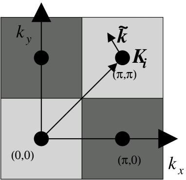
Figure 1: Schematic of the dynamical cluster approximation. The Brillouin zone is split into sub-zones, within which the self-energy is assumed to be constant. The centers of the zones are at the momenta $\boldsymbol{K}_{i}$ and a vector $\tilde{\boldsymbol{k}}$ is defined which relates the center of a sub-zone to a location in that sub-zone.

By neglecting momentum conservation at the interaction vertices, DMFT replaces the self-energy, $\Sigma(\boldsymbol{k},\omega)$, by its momentum-independent counterpart. In 2D, the spatial fluctuations which were neglected in the DMFT are expected to contribute significantly. DCA includes these fluctuations by dividing up the Brillouin zone into sub-zones which obey the lattice symmetry M.H.Hettler et al. (1998) or more recently using Bett’s clusters Kent et al. (2005). This coarse graining step corresponds to a mapping onto a cluster-impurity model. Within each of these sub-zones, the self-energy is assumed to be momentum independent, so the coarse graining of the Green function can be written

$$G(\boldsymbol{K}_{i},z)=\sum_{\tilde{\boldsymbol{k}}}\frac{1}{z-\epsilon(\boldsymbol{K}_{i}+\tilde{\boldsymbol{k}})-\Sigma(\boldsymbol{K}_{i},z)}\,.$$ (1)

Here $\tilde{\boldsymbol{k}}$ is a vector that lies within the sub-zone as shown in Fig. 1. The sum over momenta is normally carried out numerically.

Since the self-energy is momentum independent within each sub-zone, it is possible to replace the sum over momenta with a partial density of states, leading to the relation M.H.Hettler et al. (1998),

$$G(\boldsymbol{K}_{i},z)=\int_{-\infty}^{\infty}\frac{D_{\boldsymbol{K}_{i}}(\epsilon)\,d\epsilon}{z-\epsilon-\Sigma(\boldsymbol{K}_{i},z)}\,,$$ (2)

where $D_{\boldsymbol{K}_{i}}(\epsilon)$ is the non-interacting fermion partial density of states (DOS) for the sub-zone centered about $\boldsymbol{K}_{i}$ (see figure 2(a)).

In both DMFT and DCA, the self-energy and the coarse-grained Green function are also related through a modified Dyson equation,

$${\mathcal{G}}_{0}^{-1}(\boldsymbol{K}_{i},z)-G^{-1}(\boldsymbol{K}_{i},z)=\Sigma(\boldsymbol{K}_{i},z)\,.$$ (3)

The self-consistency is closed by calculating the self-energy from ${\mathcal{G}}_{0}(\boldsymbol{K}_{i},z)$, which may be interpreted as the host Green function of an impurity model Georges et al. (1996). Cluster impurity problems have been extensively studied, therefore a number of different approximations for the self-energy are readily available.

Here, I suggest a simple analytical form for the dynamical-cluster self-consistency step, Eqn. 2. I use results from the Hubbard model J.Hubbard (1963) to establish if the simplified forms lead to acceptable results. The Hubbard model is one of the simplest non-trivial models of electronic correlations in the solid state, and examines a single band of electrons, hopping between lattice sites with amplitude $t$, and interacting via a Coulomb repulsion, $U$, represented by a Hamiltonian,

$$H=-\sum_{<ij>\sigma}t_{ij}c^{\dagger}_{i\sigma}c_{j\sigma}+U\sum_{i}n_{i\uparrow}n_{i\downarrow}$$ (4)

($c^{\dagger}_{i\sigma}$ creates an electron on site $i$ with spin $\sigma$ and $n_{i\sigma}$ is the number operator). This model can only be solved exactly in one dimension E.H.Lieb and Wu (1968), but has been extensively examined in the infinite-dimensional limit corresponding to DMFT Georges et al. (1996), and in a wide range of other approximations, including DCA Maier et al. (2005).

This paper is set out as follows: In section II, I suggest and summarize several approximate forms for the self-consistency step of the DCA equations. I test the accuracy of the new schemes in section III. Possible extension for two-particle properties is discussed in section IV and for multiple bands in section V. A brief discussion can be found in section VI.

II Analytical approximations to DCA

Table 1: Offsets and widths of the partial DOS for a 2D tight-binding square lattice to be used as input for the various schemes. First and second moments of the irreducible partial densities of states are used to calculate these values up to cluster sizes of $N_{c}=8$ ($W=4t$ is the half band-width).

$N_{C}$	$\boldsymbol{K}_{i}=(k_{x},k_{y})$	Offset ($\bar{\epsilon}_{\boldsymbol{K}_{i}}/W$)	Width ($t_{i}/W$)
1	$(0,0)$	0.000	0.500
2	$(0,0)$	0.405	0.293
	$(\pi,\pi)$	-0.405	0.293
4	$(0,0)$	0.637	0.218
	$(\pi,0),(0,\pi)$	0.000	0.218
	$(\pi,\pi)$	-0.637	0.218
8	$(0,0)$	0.811	0.112
	$(\pi/2,\pi/2),(3\pi/2,\pi/2),$
	$(\pi/2,3\pi/2),(3\pi/2,3\pi/2)$	0.000	0.386
	$(\pi,\pi)$	-0.811	0.112
	$(\pi,0),(0,\pi)$	0.000	0.181

An appealing aspect of DMFT is its potential for analytic work. Three forms for the non-interacting density of states are commonly used: (1) a Gaussian, which corresponds to a hyper-cubic lattice with high dimensionality, (2) a semicircular density of states which relates to a Bethe lattice with large coordination number and (3) a Lorentzian, which decouples the self-consistent equations linking DMFT with the Anderson impurity model. In the case of the DCA, the non-interacting partial density of states (partial DOS) has a complicated form, which prevents easy analytic work. In the very large cluster limit each partial DOS tends towards a $\delta$-function form. Thus in principle, any approximate partial DOS with the properties of a $\delta$ function has the correct large cluster behavior (for example one might replace the partial DOS with a Gaussian). One may go further and match the mean ($\bar{\epsilon}_{\boldsymbol{K}_{i}}$) and variance ($t_{i}=\sqrt{\bar{\epsilon^{2}}_{\boldsymbol{K}_{i}}-(\bar{\epsilon}_{\boldsymbol{K}_{i}})^{2}}$) for the approximate and exact partial DOS, to get the correct large cluster asymptotic behavior (since the low order moments dominate the form of the self-consistent condition in that case). Here the bar indicates an average over the momentum states in the subzone centered at $\boldsymbol{K}_{i}$. Smaller cluster sizes are likely to be most useful for analytic work of the type carried out with DMFT, thus it is of interest to determine whether such a procedure is useful when $N_{C}=4$, which is the smallest cluster size which can display low dimensional properties in 2D.

The essence of the proposed approach is shown for a cluster size of $N_{C}=4$ in figure 2 for a quasi-2D system with in plane hopping, $t_{\parallel}=25t_{\perp}$ (where $t_{\perp}$ is the inter-plane hopping). Panel (a) shows the numerically exact partial DOS for $N_{C}=4$. Panel (b) shows the replacement of the partial DOS by Gaussians which match the first 2 moments. Panel (c) shows a modified finite size approximation, which replaces the partial DOS with a delta function matching the 1st moment only. The equivalent non-interacting “densities of states” associated with a finite size calculation are shown in panel (d). With a simple approximate form for the partial density of states, the cluster Green function can easily be calculated. I propose several approximate forms for the partial DOS for which an analytic form for the self-consistent condition can be found. These are summarized for convenience in table 2, along with the analytic form of the Green function. A key feature of the approximation considered in this article is that it becomes better as cluster size increases since the second moment becomes vanishingly small, and the forms of the partial DOS converge. As such, examinations of the four-site cluster ($N_{C}=4$) represent the most challenging test of the approximate scheme.

Figure 2: Comparison between the partial non-interacting densities of states for (a) the DCA (calculated using the analytic tetrahedron method Lambin and J.P.Vigneron (1984)), (b) Gaussian approximation to the DCA self-consistency (c) modified finite size calculations and (d) finite size calculations. A cluster size of $N_{C}=4$ is shown since this is expected to be the most useful for analytic work. As the lattice size increases, the Gaussian form converges with the exact result.

Table 2: Analytic forms for the partial DOS and the corresponding self-consistent equation. $z_{i}=i\omega_{n}+\mu-\Sigma(\boldsymbol{K}_{i},i\omega_{n})$, $s=\mathrm{sgn}(\mathrm{Im}[z_{i}])$, $\mathrm{erfc}$ is the complimentary error function, $t_{i}=\sqrt{\bar{\epsilon}^{2}_{\boldsymbol{K}_{i}}-(\bar{\epsilon}_{\boldsymbol{K}_{i}})^{2}}$ and $\bar{\epsilon}_{i}$ is the average of the non-interacting dispersion over the course graining zone.

Scheme	partial DOS ($D_{i}(\epsilon)$)	Green function ($G(z_{i})$)
Gaussian	$\frac{\exp(-(\epsilon-\bar{\epsilon}_{i})^{2}/2t_{i}^{2})}{t_{i}\sqrt{2\pi}}$	$-\frac{is\sqrt{\pi}}{t_{i}\sqrt{2}}\exp\left(-\frac{(z-\bar{\epsilon}_{i})^{2}}{2t_{i}^{2}}\right)\mathrm{erfc}(-\frac{is(z-\bar{\epsilon}_{i})}{t_{i}\sqrt{2}})$
Semi-circular	$\frac{\sqrt{4t_{i}^{2}-(\epsilon-\bar{\epsilon}_{i})^{2}}}{2\pi t_{i}^{2}}$ ($|\bar{\epsilon_{i}}-\epsilon|<2t_{i}$)	$\frac{z_{i}-\bar{\epsilon}_{i}-s\sqrt{(z_{i}-\bar{\epsilon}_{i})^{2}-4t_{i}^{2}}}{2t_{i}^{2}}$
Square	$\frac{1}{2t_{i}\sqrt{3}}\hskip 8.53581pt(|\epsilon-\bar{\epsilon}_{i}|<t_{i}\sqrt{3})$	$\frac{1}{2t_{i}\sqrt{3}}\ln\left[\frac{z-\bar{\epsilon_{i}}-t_{i}\sqrt{3}}{z-\bar{\epsilon_{i}}+t_{i}\sqrt{3}}\right]$
Lorentzian	$\frac{t_{i}}{\pi((\epsilon-\bar{\epsilon}_{i})^{2}+t_{i}^{2})}$	$\frac{1}{z_{i}-\bar{\epsilon}_{i}+it_{i}\mathrm{sgn}(\mathrm{Im}[z_{i}])}$
Modified FS	$\delta(\epsilon-\bar{\epsilon}_{i})$	$\frac{1}{z-\bar{\epsilon}_{i}}$

The Gaussian approximation to the partial DOS has the advantage that the full moment expansion is uniquely defined by the first two moments in the expansion, so all moments are well defined. However, the form of the Green function is relatively complicated, involving a complimentary error function. The semi-circular and square partial DOS are bounded, as is the case for all partial DOS in low dimensional systems, and lead to a Green function with a simple analytic form (i.e. the self-consistent equation can be inverted in terms of common functions). The first and second moments of the partial DOS are matched in all of these schemes. The square DOS approximation is not tested here.

There are two additional schemes that have some potential for analytic calculations. The first is the Lorentzian approximation. For $N_{C}=1$ this corresponds to the solution of an Anderson impurity model, and as such the self-consistent equations are decoupled. The second treats the partial DOS as a $\delta$-function, where only the 1st moment is matched. This is similar to using a finite size (FS) technique, except that the shift in the peak location from the original position involves a large number of states, and such an approximation has aspects of both the thermodynamic limit of a large number of states and of finite size simulations.

III Numerical test of applicability

Figure 3: Comparison between the DCA and the approximate DCA schemes for thermodynamic quantities, using FLEX as a cluster solver and with a cluster size $N_{c}=4$. Panel (a) shows the variation of the local moment ($\langle L_{0}\rangle$) with coupling, and panel (b) shows the variation of the total energy, $E_{\mathrm{tot}}$, with coupling. The temperature for these calculations is $T=0.04W$ and the density of electrons per site, $n=1$. The Gaussian approximation to the DCA self-consistency leads to results which are almost indistinguishable from those calculated using the exact partial DOS (the open and filled circles lie on top of each other). The semi-circular approximation to the partial DOS also leads to good results. It is very important for the 1st and 2nd moments of the partial densities of states to match, or there are significant inconsistencies, such as those seen using the modified finite size approximation and Lorentzian DOS. For methods with matching moments, agreement is almost exact for $U\gtrsim W$.

Figure 4: Variation of filling with chemical potential showing the performance of the scheme away from half filling. $T=0.04W$ and $U=2W$. Agreement is good for filling less than $n=1.5$, where a kink develops. For larger fillings, there are small discrepancies of the order of a few percent. This is expected, since the Gaussian form of the partial DOS has unphysical long tails, where the exact partial DOS has a sharp cutoff.

Figure 5: Real and imaginary parts of the Green function on the Matsubara axis. Values are in agreement to within 1%. $U=0.5W$, $N_{c}=4$ and $T=0.04W$ and the system is half filled.

Figure 6: Comparison of real and imaginary parts of the Green function on the Matsubara axis. Parameters are as Fig. 5.

Figure 7: Comparison of the density of states computed using a Padé approximant analytic continuation of order 800. While the detailed structure of the interacting DOS varies slightly, the main features are similar. This is in spite of the significant difference between the exact and approximate forms of the non-interacting density of states at the Fermi-surface. Parameters are as Fig. 5.

This section assesses the applicability of the approach described in the last section. The accuracy of the results computed using the approximate self-consistent step is considered as a function of the Hubbard $U$. Values of the Hubbard $U$ approaching the band-width will be considered. In this paper, numerics are used to demonstrate the validity of the scheme. However, the intention is that researchers will be able to use approximate forms of the self-consistent condition to generate analytic solutions of model systems in conjunction with appropriate forms of the self energy.

In order to test the accuracy of a scheme which uses approximate partial densities of states, the fluctuation-exchange (FLEX) approximation is used to compute the self energy of the cluster. Details of the FLEX approach and its use as a cluster solver may be found elsewhere N.E.Bickers and D.J.Scalapino (1989); K.Aryanapour et al. (2002). FLEX has a transparent physical interpretation, since it approximates the self-energy by three subsets of diagrams, which represent spin-flips, density fluctuations and pair fluctuations. Computations were carried out at finite temperature using the Matsubara formalism. All calculations were initialized with zero self-energy, and then the Green function was calculated self-consistently until a convergence of 1 part in $10^{6}$ was reached. At this stage, observables were calculated. Ideally a full quantum Monte-Carlo scheme would be used to solve the cluster impurity problem, since FLEX can overestimate the self-energy and could potentially be insensitive to the different forms of the course graining schemes (for example the absence of van Hove singularities). However for moderate couplings FLEX is accurate, and it is expected that approximate schemes for the self-consistency are most likely to fail when electrons are not localized (since strongly localized electrons can be well described with a single site impurity).

The total energy and local moment are plotted in figure 3 as coupling, $U$, is varied. The cluster size is $N_{C}=4$, temperature $T=0.04W$ and electron density $n=1$. Results computed using a number of different approximations to the partial DOS are shown. The Gaussian approximation to the partial DOS leads to the most accurate results. In fact, the difference between the curves computed using the Gaussian and exact non-interacting DOS is not easily distinguished by eye. Agreement is also found when the semi-circular partial DOS is used to approximate the self-consistency, with an accuracy of a few percent. Using the semi-circular DOS to approximate the self consistency is more favorable to analytic approximations, since the self-consistent equations also have a square root form and can easily be inverted. At large $U$, the curves corresponding to the Gaussian DOS, semi-circular DOS and the DCA scheme all converge. This is expected, since at large $U$ at half-filling hopping is suppressed, the system becomes local and the precise form of the non-interacting DOS (which is related to the details of the intersite hopping and the specific lattice) becomes irrelevant.

The matching of both moments is very important to achieve accurate results. When only the first moment is matched, for example using the modified finite size approximation, the errors on the moment and total energy are significant. There is a large overestimation of the local moment, and a huge underestimation of the total energy. Approximating the exact non-interacting density of states with a Lorentzian generates the worst approximation. Presumably this is because the second moment is ill defined, and the kinetic energy in the absence of interaction is grossly overestimated. However, some of the qualitative features remain and it might be possible to extract some useful physics even with such a crude approximation Georges et al. (1996).

The previous results were calculated for a half filled lattice, corresponding to one of the interesting limits of the Hubbard model. To determine the performance of the approximation away from half-filling, figure 4 shows the variation of the filling as the chemical potential, $\mu$, is changed. The temperature is $T=0.04W$ and the coupling $U=2W$. Calculations are shown for the full DCA self consistency scheme, and also for the Gaussian and semi-circular approximations to the self-consistency. The change of $n$ gives a rough measure of the variation in the renormalized DOS at the Fermi energy for a particular value of the chemical potential, and thus an indication of the performance of the scheme away from half filling. For $n\neq 1$, it might be expected that the analytic schemes have larger errors, since the approximate forms of the non-interacting DOS do not have the correct form when the density of electrons is low (for example the Gaussian DOS has unphysical high energy tails). In fact, the agreement is good for filling less than $n=1.5$, where a kink develops. For larger fillings, there are only small discrepancies of the order of a fraction of a percent.

Since it is possible that cancellations of errors could lead to good agreement of thermodynamic quantities, but may not give good results when correlation functions are computed, Fig. 5 shows the real and imaginary components of the Green function on the Matsubara axis. Only tiny differences can be seen between the forms of the Green functions computed using the Gaussian approximated scheme and the DCA. Here $U=0.5W$, $N_{c}=4$ and $T=0.04W$ and the system is half filled. To clarify the quality of the approximation, the difference between the values of the Green functions is shown in Fig. 6. For the parameters used here, the difference is around 1% for the smallest Matsubara frequencies, and the two schemes converge for larger values of $\omega_{n}$. In the weak to intermediate $U$ regime, any discrepancies between quantities computed using the approximate and exact forms of the self-consistency condition are expected to be most pronounced, and intermediate $U$ is of most physical interest, so it is promising that the approximate scheme works well for $U=0.5W$.

Finally, to demonstrate that the form of the interacting density of states $A(\omega)=-{\rm Im}[G(\omega+i\eta)]/\pi$ can be computed to reasonable accuracy using the alternative self consistency scheme, Padé approximants are used to analytically continue the Green function to the real axis Vidberg and Serene (1977) as shown in Fig. 7. While the detailed structure of the interacting DOS varies slightly, the main features are similar. This is in spite of the significant difference between the exact and approximate forms of the non-interacting density of states at the Fermi-surface (for example, a factor of almost 2 difference can be seen at the Fermi surface in Fig. 2). In particular, a similar amount of spectral weight is shifted across the Fermi surface in both cases. The density of states at the Fermi-surface associated with the course grained zone centered about the $(\pi,0)$ point is of similar size for both approximations, and the band widening is similar.

IV Extension to two-particle properties.

In principle, the analytic schemes presented here could be used for calculating two particle properties, such as the superconducting, charge density wave and spin density wave susceptibilities. To examine the potential for the computation of two particle properties, I use the particle-hole susceptibility as an example. Following Ref. Jarrell et al., 2001, the coarse-grained non-interacting susceptibility can be computed using the following expression,

$$\bar{\chi}^{0}_{\sigma\sigma^{\prime}}[(\boldsymbol{q},i\nu_{s});(\boldsymbol{K}_{i},i\omega_{n})(\boldsymbol{K}_{j},i\omega_{m})=\delta_{\sigma\sigma^{\prime}}\delta_{ij}\delta_{nm}\sum_{\tilde{\boldsymbol{k}}}G_{\sigma}(\boldsymbol{K}_{i}+\tilde{\boldsymbol{k}},i\omega_{n})G_{\sigma}(\boldsymbol{K}_{i}+\tilde{\boldsymbol{k}}+\boldsymbol{q},i\omega_{n}+i\nu_{s})\,,$$ (5)

where $\tilde{\boldsymbol{k}}$ is a vector that lies within a sub-Brillouin zone. It is possible to simplify this expression for use with the approximate scheme discussed in this article in two special cases; when $\boldsymbol{q}=\boldsymbol{0}=(0,0,\cdots)$ and when $\boldsymbol{q}=\boldsymbol{\pi}=(\pi,\pi,\cdots)$. First, if $\boldsymbol{q}=\boldsymbol{0}$ then the propagator becomes,

$$\bar{\chi}^{0}_{\sigma\sigma^{\prime}}[(\boldsymbol{0},i\nu_{s});(\boldsymbol{K}_{i},i\omega_{n})(\boldsymbol{K}_{j},i\omega_{m})=\delta_{\sigma\sigma^{\prime}}\delta_{ij}\delta_{nm}\times$$ (6)

$$\sum_{\tilde{\boldsymbol{k}}}\frac{1}{i\omega_{n}+\mu-\epsilon(\boldsymbol{k})-\Sigma(i\omega_{n},\boldsymbol{K}_{i}+\tilde{\boldsymbol{k}})}\frac{1}{i\omega_{n}+i\nu_{s}+\mu-\epsilon(\boldsymbol{k})-\Sigma(i\omega_{n}+i\nu_{s},\boldsymbol{K}_{i}+\tilde{\boldsymbol{k}})}\,.$$

Since in the dynamical cluster approximation $\Sigma$ is constant within each sub-zone, this simplifies to,

$$\bar{\chi}^{0}_{\sigma\sigma^{\prime}}[(\boldsymbol{0},i\nu_{s});(\boldsymbol{K}_{i},i\omega_{n})(\boldsymbol{K}_{j},i\omega_{m})=\delta_{\sigma\sigma^{\prime}}\delta_{ij}\delta_{nm}\times$$ (7)

$$\int\frac{D_{\boldsymbol{K}_{i}}(\epsilon)}{(i\omega_{n}+\mu-\epsilon-\Sigma(i\omega_{n},\boldsymbol{K}_{i}))(i\omega_{n}+i\nu_{s}+\mu-\epsilon-\Sigma(i\omega_{n}+i\nu_{s},\boldsymbol{K}_{i}))}\,,$$

so that the form of the partial density of states consistent with the approximation to the self-consistent equation can be used. Equation 7 is appropriate for all forms of lattice.

Simplifications can also be made in the more useful case where $\boldsymbol{q}=\boldsymbol{\pi}$ if there is particle-hole symmetry, for example if the lattice is square (or hypercubic) and only has near-neighbor hopping. Then $\epsilon(\boldsymbol{k})=-t\sum_{n=1}^{d}\cos(k)$, so $\epsilon(\boldsymbol{k}+\boldsymbol{\pi})=-\epsilon(\boldsymbol{k})$, and the susceptibility simplifies to

$$\bar{\chi}^{0}_{\sigma\sigma^{\prime}}[(\boldsymbol{\pi},i\nu_{s});(\boldsymbol{K}_{i},i\omega_{n})(\boldsymbol{K}_{j},i\omega_{m})=$$ (8)

$$\delta_{\sigma\sigma^{\prime}}\delta_{ij}\delta_{nm}\int\frac{D_{\boldsymbol{K}_{i}}(\epsilon)}{(i\omega_{n}+\mu-\epsilon-\Sigma(i\omega_{n},\boldsymbol{K}_{i}))(i\omega_{n}+i\nu_{s}+\mu+\epsilon-\Sigma(i\omega_{n}+i\nu_{s},\boldsymbol{K}_{i}+\boldsymbol{\pi}))}.$$

The two particle cluster susceptibility $\chi_{c,\sigma\sigma^{\prime}}[(\boldsymbol{q},i\nu_{s});(\boldsymbol{K}_{i},i\omega_{n})(\boldsymbol{K}_{j},i\omega_{m})]$ is computed in a manner which is specific to the cluster solver that is used, and does not involve any coarse graining. Once the cluster properties have been computed, the coarse grained lattice susceptibility can be computed using,

$$\bar{\chi}^{-1}=\chi_{c}^{-1}-[\chi_{c}^{0}]^{-1}+[\bar{\chi}^{0}]^{-1}\,,$$ (9)

from which the spin and charge susceptibilities can be computed Jarrell et al. (2001). Calculation of $\chi_{c}$ is quite involved in the FLEX scheme and is not discussed here.

V Multiple bands

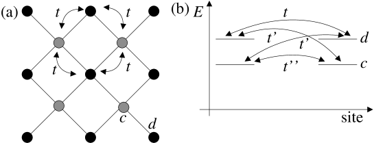
Figure 8: Possible hopping scenarios for multiband models that can be treated using the approximate self-consistent scheme (a) two bands arise from sites of different energies in a lattice with a basis of two atoms (b) two bands arise from hopping between electrons in different orbitals.

I complete this article with a discussion of the applicability of the approximate scheme to multiple bands. I consider only two bands here, but similar arguments will be applicable when there are more than two bands. A very generic two-band Hamiltonian has the form,

$$H_{2}=\sum_{\boldsymbol{k}}\epsilon_{\boldsymbol{k}}c^{\dagger}_{\boldsymbol{k}}c_{\boldsymbol{k}}+\zeta_{\boldsymbol{k}}d^{\dagger}_{\boldsymbol{k}}d_{\boldsymbol{k}}+\gamma_{\boldsymbol{k}}(c^{\dagger}_{\boldsymbol{k}}d_{\boldsymbol{k}}+d^{\dagger}_{\boldsymbol{k}}c_{\boldsymbol{k}})(+\,H_{2,\rm int})\,,$$ (10)

where $c^{\dagger}$ and $d^{\dagger}$ create electrons of distinct types (either on different atoms of a two-atom basis, or in different orbitals of a single atom). $\epsilon_{\boldsymbol{k}}$ is the electronic dispersion generated from hopping of electrons of type $c$, and $\zeta_{\boldsymbol{k}}$ corresponds to electrons of type $d$. The dispersions $\epsilon_{\boldsymbol{k}}$ and $\zeta_{\boldsymbol{k}}$ typically correspond to hopping between orbitals of the same type on different sites as shown schematically as hops of amplitude $t$ and $t^{\prime\prime}$ in Fig. 8(b). $\gamma_{\boldsymbol{k}}$ is the dispersion of electrons that hop between different types of atom such as might be found in crystals with a two-atom basis (shown schematically in Fig. 8(a)). Dispersion of type $\gamma_{\boldsymbol{k}}$ can also originate from hopping between orbitals of different types on neighboring sites, as shown schematically as hops of amplitude $t^{\prime}$ in Fig. 8(b). $H_{2,\rm int}$ contains all the interaction terms between electrons of types $c$ and $d$ within the cell.

Diagonalization of the quadratic terms using a standard Bogoliubov transformation yields,

$$H_{2}=E^{(\alpha)}_{\boldsymbol{k}}\alpha^{\dagger}_{\boldsymbol{k}}\alpha_{\boldsymbol{k}}+E^{(\beta)}_{\boldsymbol{k}}\beta^{\dagger}_{\boldsymbol{k}}\beta_{\boldsymbol{k}}\,(+H_{2,\rm int})\,,$$ (11)

where,

$$E^{(\alpha),(\beta)} = \left[\frac{\epsilon_{\boldsymbol{k}}}{2}\left(1\pm\frac{\epsilon_{\boldsymbol{k}}-\zeta_{\boldsymbol{k}}}{\sqrt{4\gamma_{\boldsymbol{k}}^{2}+(\epsilon_{\boldsymbol{k}}-\zeta_{\boldsymbol{k}})^{2}}}\right)+\frac{\zeta_{\boldsymbol{k}}}{2}\left(1\mp\frac{\epsilon_{\boldsymbol{k}}-\zeta_{\boldsymbol{k}}}{\sqrt{4\gamma_{\boldsymbol{k}}^{2}+(\epsilon_{\boldsymbol{k}}-\zeta_{\boldsymbol{k}})^{2}}}\right)\right.$$ (12)

$$\hskip 85.35826pt\left.\pm\frac{2\gamma_{\boldsymbol{k}}^{2}}{\sqrt{4\gamma_{\boldsymbol{k}}^{2}+(\epsilon_{\boldsymbol{k}}-\zeta_{\boldsymbol{k}})^{2}}}\right]\,,$$

$c^{\dagger}_{\boldsymbol{k}}=u_{\boldsymbol{k}}\alpha^{\dagger}_{\boldsymbol{k}}+v_{\boldsymbol{k}}\beta^{\dagger}_{\boldsymbol{k}}$, $d^{\dagger}_{\boldsymbol{k}}=-v_{\boldsymbol{k}}\alpha^{\dagger}_{\boldsymbol{k}}+u_{\boldsymbol{k}}\beta^{\dagger}_{\boldsymbol{k}}$, $u_{\boldsymbol{k}}^{2}=(1+A_{\boldsymbol{k}})/2$, $v_{\boldsymbol{k}}^{2}=(1-A_{\boldsymbol{k}})/2$, $u_{\boldsymbol{k}}v_{\boldsymbol{k}}=\sqrt{1-A_{\boldsymbol{k}}^{2}}/2$ and $A_{\boldsymbol{k}}=(\epsilon_{\boldsymbol{k}}-\zeta_{\boldsymbol{k}})/\sqrt{4\gamma_{\boldsymbol{k}}^{2}+(\epsilon_{\boldsymbol{k}}-\zeta_{\boldsymbol{k}})^{2}}$. The non-interacting Matsubara Green functions for $\tau>0$ form a $2\times 2$ matrix with the elements, $G^{(0)}_{cc}(\boldsymbol{k},\tau)=-\langle c_{\boldsymbol{k}}(\tau)c^{\dagger}_{\boldsymbol{k}}(0)\rangle$ and $G^{(0)}_{cd}(\boldsymbol{k},\tau)=-\langle c_{\boldsymbol{k}}(\tau)d^{\dagger}_{\boldsymbol{k}}(0)\rangle$ etc. which can be computed by substituting the Bogoliubov transformation (since $\alpha$ and $\beta$ excitations have a Fermi-Dirac distribution). After Fourier transformation,

$$G^{(0)}_{cc}(\boldsymbol{k},i\omega_{n})=\left[\frac{u_{\boldsymbol{k}}^{2}}{i\omega_{n}-E^{(\alpha)}_{\boldsymbol{k}}}+\frac{v_{\boldsymbol{k}}^{2}}{i\omega_{n}-E^{(\beta)}_{\boldsymbol{k}}}\right]$$ (13)

and

$$G^{(0)}_{cd}(\boldsymbol{k},i\omega_{n})=\frac{u_{\boldsymbol{k}}v_{\boldsymbol{k}}\left[E^{(\alpha)}_{\boldsymbol{k}}-E^{(\beta)}_{\boldsymbol{k}}\right]}{(i\omega_{n}-E^{(\alpha)}_{\boldsymbol{k}})(i\omega_{n}-E^{(\beta)}_{\boldsymbol{k}})}.$$ (14)

When interaction is switched on, the coarse grained Green function is,

$$\boldsymbol{G}=\sum_{\tilde{\boldsymbol{k}}}\boldsymbol{G}_{0}\left[1+\boldsymbol{G}_{0}\boldsymbol{\Sigma}\right]^{-1}$$ (15)

where the self-energy, $\boldsymbol{\Sigma}$, is also a $2\times 2$ matrix. As in the one-band case, the self-energy is constant within each sub-zone.

In contrast to the one-band case, the sum on $\tilde{\boldsymbol{k}}$ cannot always be replaced by a density of states. This is because $\epsilon_{\boldsymbol{k}}$, $\zeta_{\boldsymbol{k}}$ and $\gamma_{\boldsymbol{k}}$ do not normally have the same form. Under certain conditions it is possible to make the replacement and therefore use the analytic forms of the self-consistency considered in this article. In the first case, bands with dispersion $\gamma_{\boldsymbol{k}}$ are formed via nearest-neighbor hops in a system with a basis of two atoms, and $\epsilon_{\boldsymbol{k}}$ and $\zeta_{\boldsymbol{k}}$ are flat, representing the energies of the atomic sites. Then the sum over momenta is replaced by an integral over the density of states corresponding to $\gamma_{\boldsymbol{k}}$, which can then be replaced using one of the simplified analytic forms considered in section II. I note that two-band systems of this type have been studied using DMFT Georges et al. (1993).

The sum over momenta can also be replaced with an integral over a density of states when $\epsilon_{\boldsymbol{k}}\propto\zeta_{\boldsymbol{k}}$, $\epsilon_{\boldsymbol{k}}\propto\gamma_{\boldsymbol{k}}$ or $\zeta_{\boldsymbol{k}}\propto\gamma_{\boldsymbol{k}}$ (up to an offset) so long as any other dispersions are flat. This is possible for electrons moving between atoms with several orbitals by nearest neighbor hopping only (the hopping integrals can be different) as shown schematically in Fig. 8(b). Then the density of states corresponding to only one of the dispersions can be used, since any dispersion can be represented in terms of the other dispersion. In general systems with next-nearest neighbor hopping are excluded from this argument unless there are good grounds for expecting the ratio of nearest to next-nearest neighbor hopping integrals to be identical for every band. There may be other more complicated non-linear maps between dispersions (e.g. $\epsilon_{\boldsymbol{k}}=F(\gamma_{\boldsymbol{k}})$ where $F$ is an arbitrary function) so that the same trick can be applied, however the mapping must be $\boldsymbol{k}$ independent so such mappings will also be special cases.

VI Summary

This paper introduced approximate schemes for the self-consistent step of the dynamical cluster approximation. In order to simplify the self-consistent step, the partial density of states used to calculate the Green function was replaced with a simple analytic form. The limitations and errors associated with the approach were tested using the FLEX approximation for the self energy. The approximate schemes were demonstrated to work well for intermediate coupling over a range of fillings.

The best approximate result comes from replacing the exact non-interacting DOS with a Gaussian. Approximating using a semi-circular partial DOS also leads to agreement of thermodynamic properties to within a few percent of the exact result. The semi-circular approximation leads to self-consistent equations with a much simpler form, which is promising for analytic work. Finally, forms such a Lorentzian and a modified finite size scheme, where only the 1st moment is matched, lead to quantitatively different results, although some of the qualitative physics remains. These schemes lead to even simpler forms for the self-consistency. Examination of the Green function and carrying out an analytic continuation demonstrate that the scheme can also compute dynamic properties to reasonable accuracy. I add the caveat that some properties of the 2D Hubbard model may show features consistent with the influence of van Hove singularities Gull et al. (2009), and such singularities are not present in the simple approximations with small cluster sizes (although they will emerge in very large clusters). In 3D, there are no divergences in the non-interacting density of states and spatial fluctuations are less relevant, so the schemes may be most effective for such problems.

Given that the analytic forms for the self-consistency introduced here work effectively, the formalism could provide a good starting point for the calculation of analytic phase diagrams and other properties in low dimensional systems where non-local fluctuations are essential (for example unconventional superconductivity such as $d$, $p$ and extended-$s$ wave which cannot be examined with the DMFT). It is hoped that this article will stimulate such studies.

VII acknowledgements

I acknowledge support from EPSRC grant no. EP/H015655/1.

References

- W.Metzner and D.Vollhardt (1989) W.Metzner and D.Vollhardt, Phys. Rev. Lett. 62, 324 (1989).
- Georges et al. (1996) A. Georges, G. Kotliar, W. Krauth, and M. Rozenburg, Rev. Mod. Phys. 68, 13 (1996).
- M.J.Rozenberg et al. (1994) M.J.Rozenberg, X.Y.Zhang, and G.Kotliar, Phys. Rev. B 49, 10181 (1994).
- M.H.Hettler et al. (1998) M.H.Hettler, A.N.Tahvildar-Zadeh, M.Jarrell, T. Pruschke, and H.R.Krishnamurthy, Phys. Rev. B 58, R7475 (1998).
- Maier et al. (2005) T. Maier, M. Jarrell, T. Pruschke, and M. H. Hettler, Rev. Mod. Phys. 77, 1027 (2005).
- Kent et al. (2005) P. Kent, M. Jarrell, T. Maier, and T. Pruschke, Phys. Rev. B 72, 060411(R) (2005).
- J.Hubbard (1963) J.Hubbard, Proc. Royal Society 276, 238 (1963).
- E.H.Lieb and Wu (1968) E.H.Lieb and Wu, Phys. Rev. Lett. 20, 1445 (1968).
- Lambin and J.P.Vigneron (1984) P. Lambin and J.P.Vigneron, Phys. Rev. B 29, 3430 (1984).
- N.E.Bickers and D.J.Scalapino (1989) N.E.Bickers and D.J.Scalapino, Ann. Phys. 193, 206 (1989).
- K.Aryanapour et al. (2002) K.Aryanapour, M.H.Hettler, and M.Jarrell, Phys. Rev. B 65, 153102 (2002).
- Vidberg and Serene (1977) H. J. Vidberg and J. W. Serene, J. Low. Temp. Phys 29, 179 (1977).
- Jarrell et al. (2001) M. Jarrell, T. Maier, C. Huscroft, and S. Moukouri, Phys. Rev. B 64, 195130 (2001).
- Georges et al. (1993) A. Georges, G. Kotliar, and W. Krauth, Z. Phys. B 92, 313 (1993).
- Gull et al. (2009) E. Gull, O. Parcollet, P. Werner, and A. J. Millis, arXiv:0909.1795 (2009).