Event Shape Analysis in ALICE

Antonio Ortiz Velasquez ⁽¹⁾, Guy Paić ⁽¹⁾
⁽¹⁾ Instituto de Ciencias Nucleares, Universidad Nacional Autónoma de México,
Apartado Postal 70-543, México D.F. 04510, México

Abstract

The jets are the final state manifestation of the hard parton scattering. Since at LHC energies the production of hard processes in proton-proton collisions will be copious and varied, it is important to develop methods to identify them through the study of their final states. In the present work we describe a method based on the use of some shape variables to discriminate events according their topologies. A very attractive feature of this analysis is the possibility of using the tracking information of the TPC+ITS in order to identify specific events like jets. Through the correlation between the quantities: thrust and recoil, calculated in minimum bias simulations of proton-proton collisions at 10 TeV, we show the sensitivity of the method to select specific topologies and high multiplicity. The presented results were obtained both at level generator and after reconstruction. It remains that with any kind of jet reconstruction algorithm one will confronted in general with overlapping jets. The present method determines areas where one does encounter special topologies of jets in an event. The aim is not to supplant the usual jet reconstruction algorithms, but rather to allow an easy selection of events allowing then the application of algorithms.

Internal Note/Physics

ALICE reference number

ALICE-INT-2009-015 version 1.0

1 Introduction

In QCD the jets are defined as cascades of consecutive emissions of partons initiated by partons from any initial hard process. The partons produce the observed hadrons due to confinement. Di-jets were discovered in 1975 in $e^{+}e^{-}$ collisions [1], the observation of three coplanar jets has provided the first experimental evidence for the existence of gluon [2, 3, 4, 5].

Event shapes measure geometrical properties of the energy flow in QCD states. Especially in the case of $e^{+}e^{-}$ collisions and Deep Inelastic Scattering, they were among the most studied QCD observables, both theoretically and experimentally. Sphericity was used at SLAC to show the evidence for the existence of jets in the annihilation process: $e^{+}e^{-}$ at energies up to 7.4 GeV in the c. m. [1]. In 1979 the collaboration MARK-J used the variable oblateness for describing processes where three prolong jets were produced at energies up to 31.5 GeV in the c. m. [2].

Of course the shape variables are calculated in terms of the final partons and they are measured in terms of the final observed hadrons, so it is possible to use them in order to do studies of corrections by hadronization effects [7, 8]. Also a vast number of strong coupling constant measurements was reported [6]. In the case of the MC generators the validation of some results were also published [10, 11].

Experimentally, jets in proton-proton collisions are defined as an excess of transverse energy over the background of the underlying events¹¹1Underlying events are formed from the beam-beam remnants, initial-state radiation and possible from soft and semi-hard multiple parton interactions. with a typical cone radius $R_{C}=1$ in $\eta-\phi$ . In ALICE we do not yet have an extensive calorimeter. For this reason, in order to define and reconstruct jets we are using tracking measurements. The jets identification is based on different algorithms; for example the cone ones. In this work we propose a method which uses the event shapes to identify interesting topologies of events like jets, which of course does not prevent the later use of jet algorithms on the selected events.

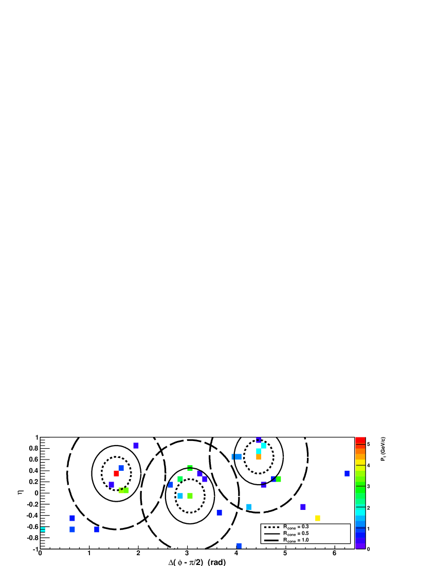
The main problem we will face at LHC is the big number of jets overlapping one another. This makes all analysis subject to numerous cuts which do increase the systematic uncertainties of the results. A typical events represented in the eta-phi plane is shown in Fig. 1. To guide the eye the contours of jets with $R_{cone}$ =0.3, 0.5 and 1 are shown for the ALICE acceptance. However in this note we would like to emphasize the fact that there is a possibility, using the event shapes, to identify painlessly events where the topology is much simpler than shown in Fig. 1. In the present note we first describe the technicalities of the method of event shape analysis giving some overview of salient topologies like events where the jets are only partially detected in the acceptance, events with 2 jets and events with 3 jets. Then, the main features of each class are studied and demonstrated, like total pt spectra of jets, the sensitivity on the parameters variation within the method, the yield of specific topologies in function of multiplicity. Finally we introduce also a bulk analysis of all events without selection. We used this to present a comparison between Pythia and PHOJET events for different parameter values.

Refer to caption — Figure 1: Plot: $\eta$ vs. $\Delta(\phi-\pi/2)$ vs. $p_{t}$ for a typical event. The leading particle is placed at $\pi/2$ rad. Different radius are shown.

2 Definitions of the shape variables

By construction the following quantities are Infra Red and Collinear (IR $\&$ C) safe. The shape variables at hadron colliders are defined over particles within the acceptance of the detector. The thrust ( $T$ ) is defined as in the $e^{+}e^{-}$ case, but using only transverse variables [12]:

T\equiv\underbrace{max}_{\overrightarrow{n}_{t}}\frac{\sum_{i}|\overrightarrow{p}_{t,i}\cdot\overrightarrow{n}_{t}|}{\sum_{i}|\overrightarrow{p}_{t,i}|}

(1)

In the literature it is more common to find the following definition:

\tau\equiv 1-T

(2)

(related to the sphericity of the event).

The range of $\tau$ is between 0 (for events with narrow back-to-back jets) and $1/2$ (for events with a uniform distribution of momentum).

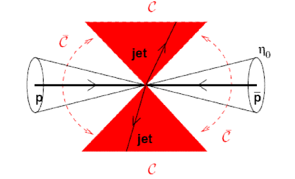
The recoil term $R$ is simply the vector sum of the transverse momentum: (Fig. 2)

R\equiv\frac{1}{\sum_{i}|\overrightarrow{p}_{t,i}|}|\sum_{i}\overrightarrow{p}_{ti}|

(3)

This quantity measures the balance of momenta of the event. For example for a di-jet event, with only one jet inside the acceptance of the detector (monojet in the further text): $R$ tends to 1, because there are no vectorial cancellations in the numerator which appear in the definition of $R$ . Otherwise, in the case of the perfect 2 back-to-back jet completely inside the acceptance: $R$ tends to 0.

3 Description of the event shape analysis (ESA)

We have computed the shape variables at level generator and reconstruction. The participants in the computations are primary charged particles ²²2Primary particles are defined as particles produced in the collision, including products of strong and electromagnetic decays, but excluding feed-down products from strange weak decays and particles produced in secondary interactions. In the simulation these are the final state particles created by the event generator, which are then propagated (and decayed) by the subsequent detector simulation. in the generation case, and tracks associated with primary particles in the reconstruction one. In both cases events are selected using the MB2³³3This trigger uses the logical AND between the V0-OR signal and the Pixel-Fast-OR. And it is an option if one needs to assign each trigger to a specific bunch crossing [14]. trigger criteria and we restrict the analysis for events with primary vertex in $z$ direction: $|v_{z}|\leq 10$ cm.

The requirements to perform the computation are:

1.
Generation level:
- Event level:
  
  the first step is for selecting hard events: $p_{t}^{leading}\geq 3$ GeV/c and $|\eta^{leading}|\leq 0.5$ . This requirement guarantees that the leading jets are contained within the ALICE acceptance with a $\Delta R_{cone}=\sqrt{\Delta\eta^{2}+\Delta\phi^{2}}\leq 0.7$
- Particle level:
  
  for primary charged particles in the acceptance: $|\eta|\leq 1$ and $p_{t}\geq 1.5$ GeV/c, the shape variables are computed. The cut in $p_{t}$ eliminates the mostly soft underlying component.
2.

Reconstruction level: In the present analysis we used tracks reconstructed by the TPC and ITS. The event cuts described above are applied.
- Track level:
  tracks associated to primary particles in the acceptance: $|\eta|\leq 1$ and with $p_{t}\geq 1.5$ GeV/c. To select this class of tracks we applied the following cuts.
  1. (a)
    
    TPC refit.
  2. (b)
    
    At least 50 clusters in TPC.
  3. (c)
    
    Covariance matrix cuts.
  4. (d)
    
    Reject kink daughters.
  5. (e)
    
    Maximum DCA (in $xy$ and $z$ ) to vertex $3$ cm.
For more details see [13].

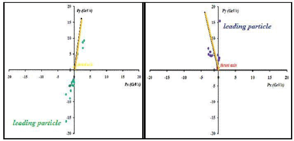
In the Fig. 3 we show a picture of two classes of candidate events: di-jet and mono-jet (to separate these events we used their values of shape variables according with the discussion in the next paragraphs). For a given event we have taken the projection of the particles momentum in the transverse plane. It is well visible that the thrust axis is very close to the direction of the transverse momenta of the leading particle (particle with the highest $p_{t}$ in the event).

The method starts by plotting a two dimensional distribution (“thrust map”), with $\tau$ ( $1-T$ ) in the horizontal axis and $R$ in the vertical axis. This plot allows to identify different classes of events according with their location in the thrust map.

1.

Region A. Suppose a di-jet event which occurs completely inside the ALICE acceptance ( $|\eta|\leq 1$ ). In this case, we have in the transverse plane; the thrust axis ( $\overrightarrow{n}_{t}$ ) almost collinear to the direction of the leading particle. So, the ratio of definition (1) tends to 1, and the recoil term tends to 0. So, the region A is characterized by events with small values of $1-T$ and $R$ , corresponding to di-jet events.
2.

Region B. Events with only one jet in the acceptance of the detector will have small values of $\tau$ and due to the absence of vectorial cancellations in the numerator of the recoil term, these classes of events will have the biggest values $R$ . So, the region B is populated by monojet events.
3.

Region C. The most isotropic events (with high $1-T$ and small $R$ ) of the sample have to compensate the transverse momentum. This zone of the thrust map is characterized by the presence of three jet events that we like to call, as at LEP, “mercedes” events.

The intermediate region between A and B is populated by the combination of mono-jets and “incomplete di-jets”; di-jets are incomplete due to their high $R$ , many particles are outside of the acceptance.

The intermediate region between B and C is populated by events were 3 or more jets are emitted but at small angles with respect to the direction of the leading jet.

In the present note we will not deal with these cases which will be the subject of a special study at later time.

4 Event shape analysis in minimum bias simulations.

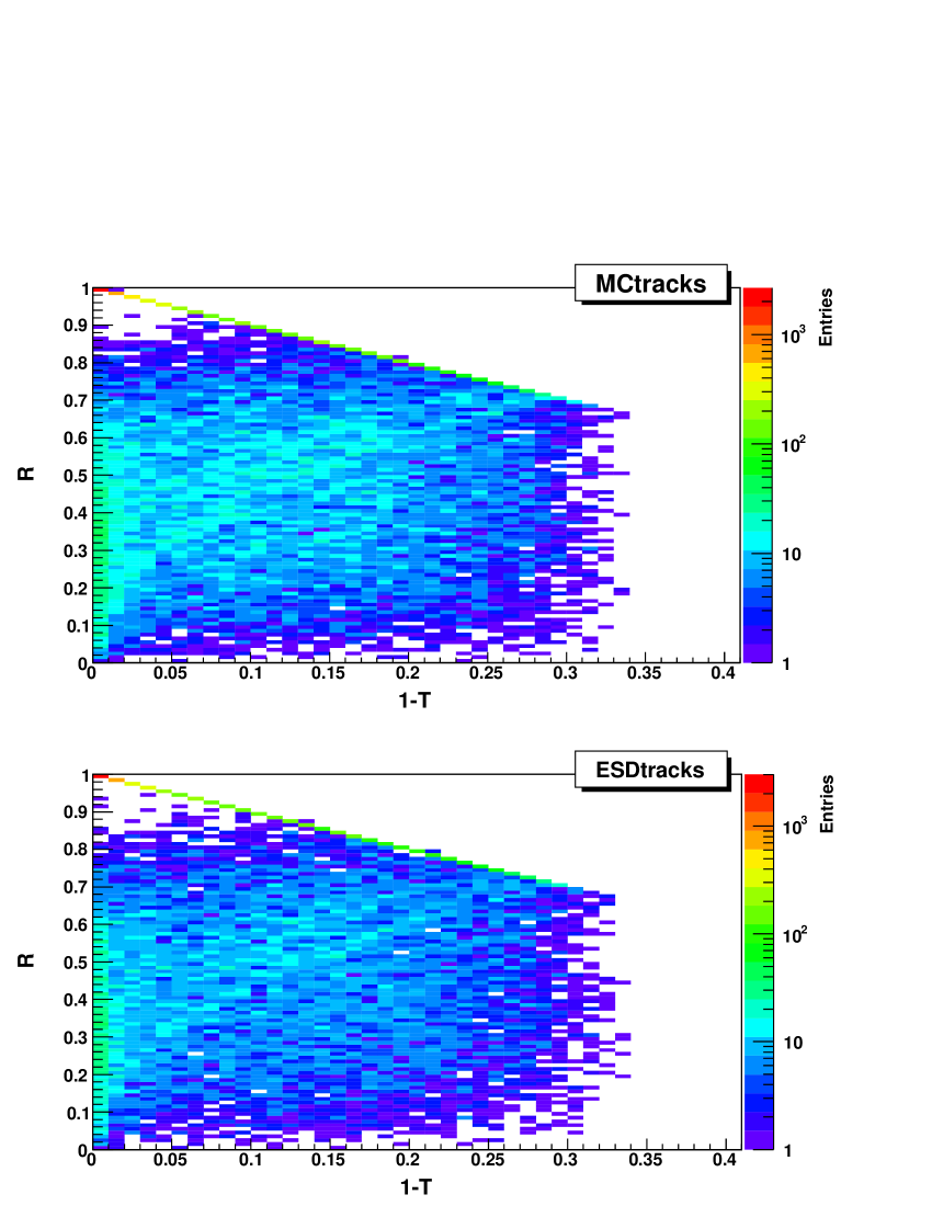
The present analysis uses the standard simulated samples staged on alicecaf⁴⁴4The CERN Analysis Facilities for ALICE (alicecaf) is a cluster at CERN running PROOF (Parallel ROOT Facility) which allows interactive parallel analysis on a local cluster.. The production corresponds to PDC09, minimum bias simulations of proton-proton collisions at 10 TeV in the center of mass, the events were generated with Pythia. The simulation of the detector included a magnetic field of 0.5 $T$ . The results were obtained through the analysis of $1,200,000$ events. In the figure 4 the thrust map is shown for generated (upper) and reconstructed (bottom) data. In both histograms two interesting regions are exhibited (A and B regions described before). Note, that any exceptional event with an azimuthally uniform distribution would be immediately “detected” in the unpopulated area: $1-T\geq 0.35$ .

The line which appears in the high R part of the map is due to the definition of the variables. For example, suppose that we have one event with a certain thrust axis $\overrightarrow{n}_{t0}$ , and in the event there are $N$ particles. If the vectorial transverse momentum of the particle $i$ is $\overrightarrow{p}_{t,i}$ , then from the definitions of R and T:

1-T+R=1-\frac{\sum_{i}|\overrightarrow{p}_{t,i}\cdot\overrightarrow{n}_{t0}|}{\sum_{i}|\overrightarrow{p}_{t,i}|}+\frac{|\sum_{i}\overrightarrow{p}_{ti}|}{\sum_{i}|\overrightarrow{p}_{t,i}|}

(4)

Now, we use the fact that:

|\sum_{i}\overrightarrow{p}_{ti}|\leq\sum_{i}|\overrightarrow{p}_{t,i}|

(5)

Then:

1-T+R\leq 1-T+1

(6)

The maximum value which $T$ can reach is 1, so we find the following restriction:

1-T+R\leq 1

(7)

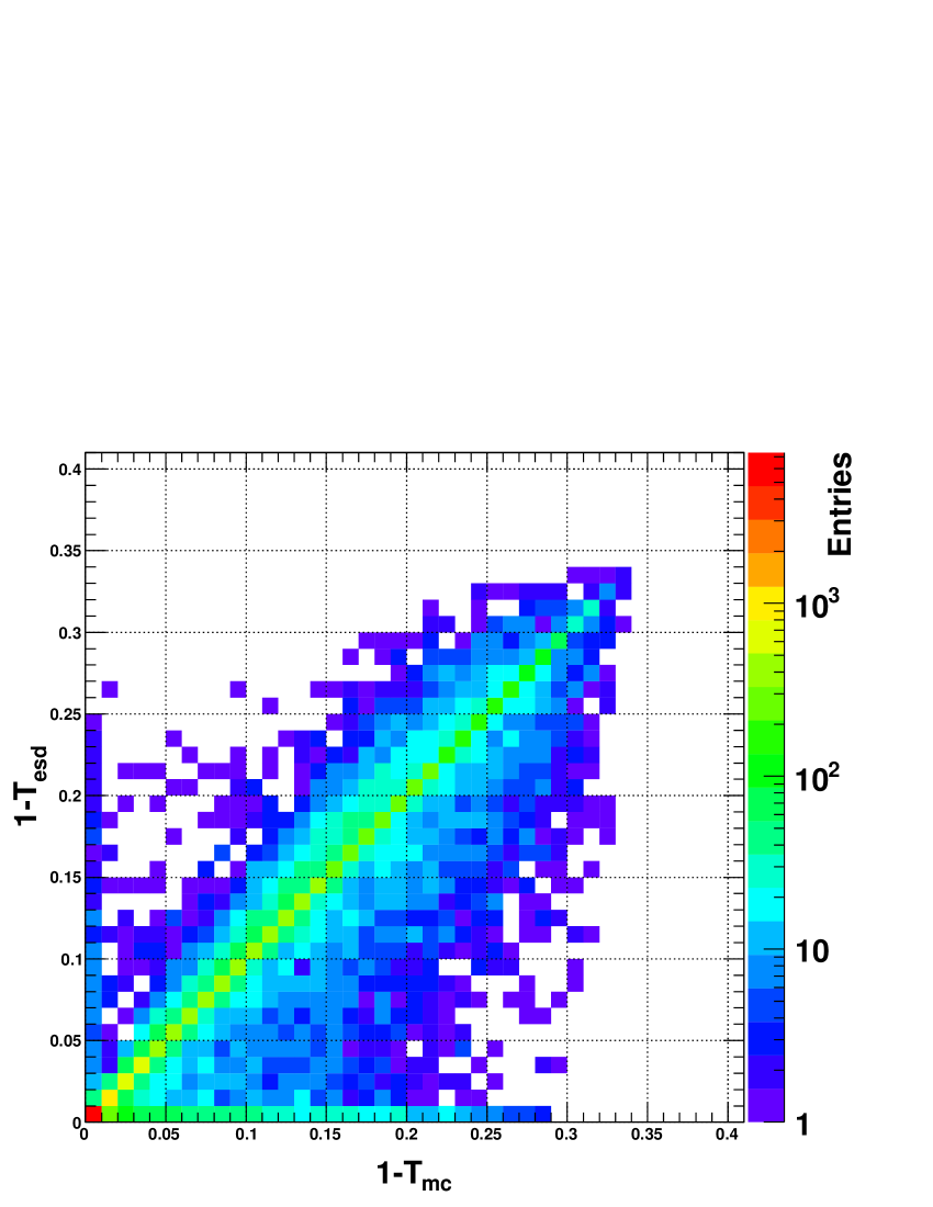
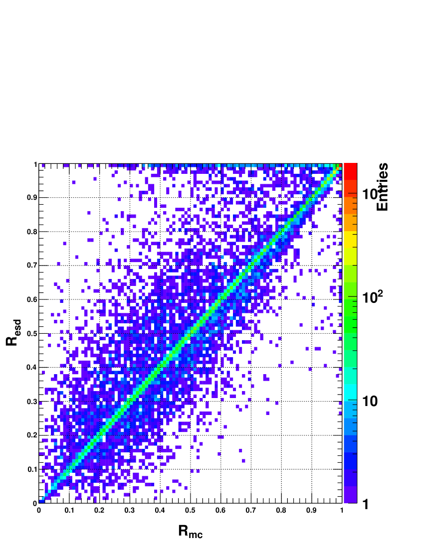
In the Fig. 5 there is a plot which shows the correlation of the $1-T$ values computed from the generator information and from the reconstruction. Note that there is a small leakage of events with $1-T_{mc}\geq 0.03$ to the reconstructed zone associated to events with 2 back-to-back jet structure. This can be understood in terms of the reconstruction effects. For example a generated event with three primary charged particles ( $p_{t}\geq 1.5$ GeV/c) distributed isotropically in the azimuth could be reconstructed as a event with a structure of two jets.

In the Fig. 6, we show the analogous plot for the variable $R$ .

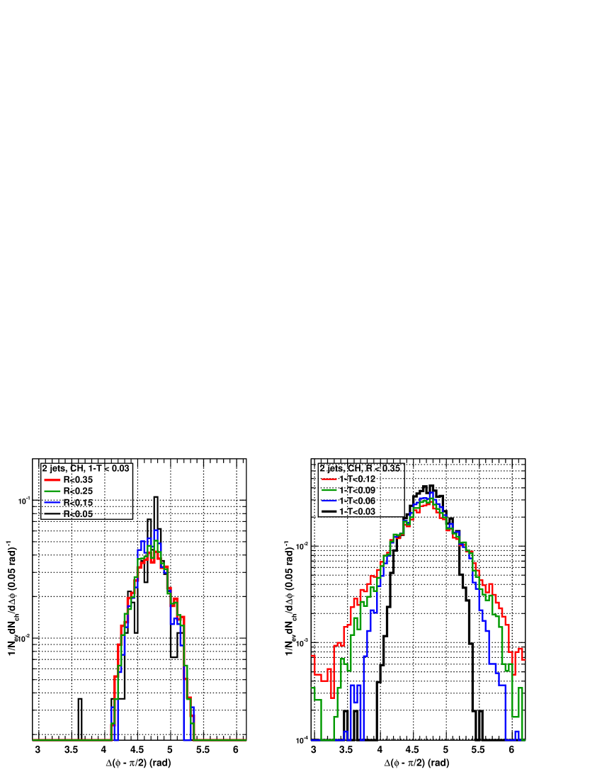
For describing the topology of the events we performed an azimuthal correlation. The idea is to select the leading particle, and apply a rotation placing it at $\pi/2$ rad. After that, we plot the azimuthal distribution of the associated particles with respect to the leading one. In the following our convention about the azimuthal correlation it will be referred as $\Delta\phi$ and it refers to: $\Delta(\phi-\pi/2)$ .

If we concentrate ourselves to events in the region $1-T\leq 0.03$ , and small $R\leq 0.35$ values. The azimuthal correlation of the Fig. 7 (right panel) shows that the width of the away side peak does not change if we modify the cut in the $R$ range. This is in agrement with our assumption which suggests that $R$ is important to select complete events in the acceptance. On the other hand, if we select events with small value of $R$ ( $R\leq 0.35$ ) and modify the range of $1-T$ (Fig. 7 (left panel)) there is a clear evolution in the structure of the away side peak. If we increase the value of $1-T$ the selected events include different configuration multijets (split jets) which are manifested in the azimuthal distribution behavior. This suggests that the cut $1-T\leq 0.03$ is almost equivalent to select particles inside a cone radii $R_{c}=\sqrt{(\Delta\phi)^{2}+(\Delta\eta)^{2}}=1$ .

In the following we will concentrate on particular parts of the map, plotting the azimuthal correlations encountered.

The procedure is:

•

Select events according to their values of shape variables as shown in table 1

Region	Kind of event	Variables
A	Dijets	$R\leq 0.35$ , $\tau\leq 0.03$
B	Monojets	$R\geq 0.9$ , $\tau\leq 0.03$
C	Mercedes	$R\leq 0.4$ , $\tau\geq 0.25$

Table 1: 1-T and R parameters used for the present analysis.

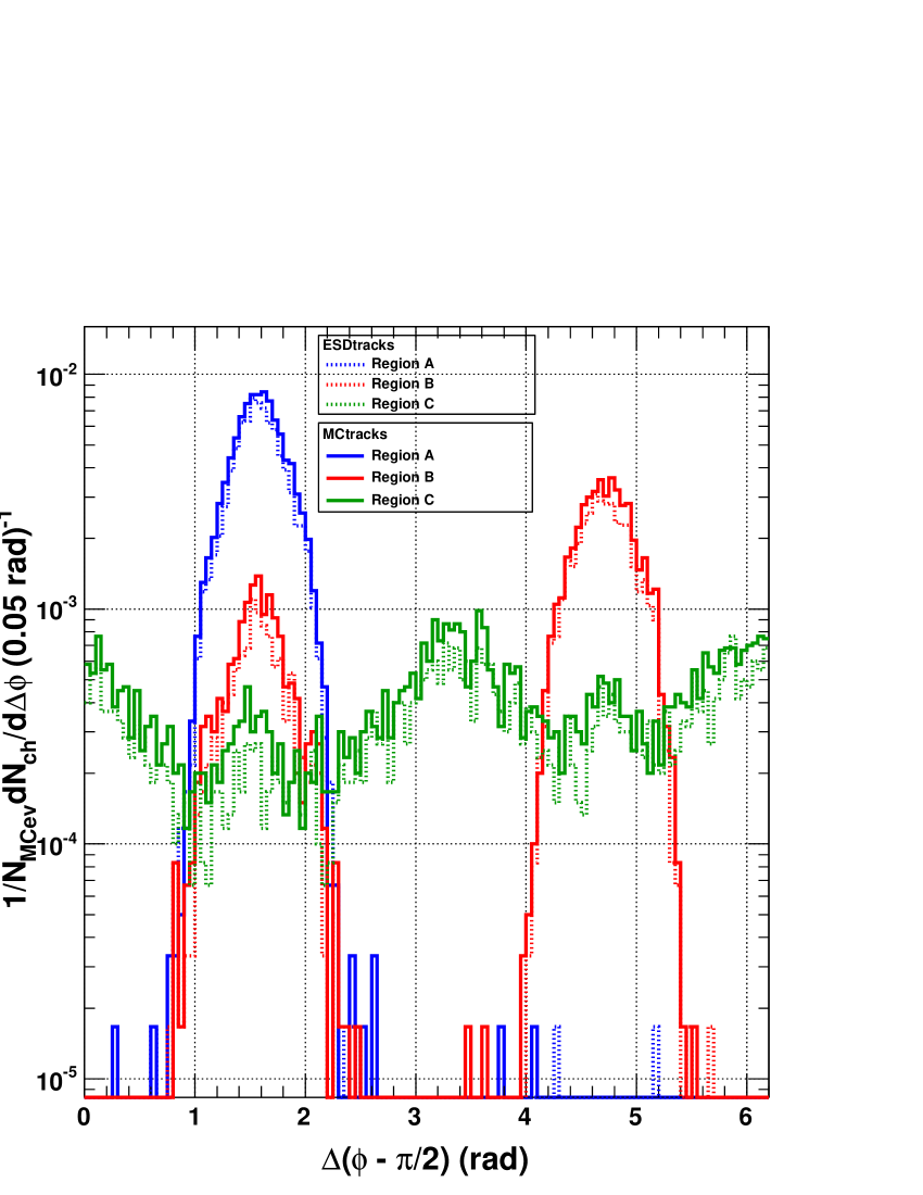
The azimuthal correlations of events sited at different regions of the thrust map are plotted in Fig. 8. The evolution of the away peak (formed by particles with $\pi\leq\Delta\phi\leq 2\pi$ ) is interesting.

As predicted, the events of region B really have a monojet topology in the azimuth. One can see there are associated particles which go near to the leading particle (peak in the toward side: $0\leq\Delta\phi\leq\pi$ ) but in the away side there is no corresponding jet. In contrast, for events of the region A the peak of the away side is located at $\Delta\phi\sim 3\pi/2$ , so, in the transverse plane we have 2 back-to-back jets. In the case of the events of region C we found a three-jet structure, in the green distribution we observe three peaks in the spectrum: the first (associated to the leading jet) at $\Delta\phi\sim\pi/2$ and the others at $\Delta\phi\sim 7\pi/6$ and $\Delta\phi\sim 11\pi/6$ respectively. Due to the observed topology we named the latter “mercedes” events. The result bears some resemblance with the away side structure observed at RHIC e.g. PHENIX collaboration in heavy-ion collisions [15]. This observation brought us to study the presence of the same double hump structure at RHIC energies [18]

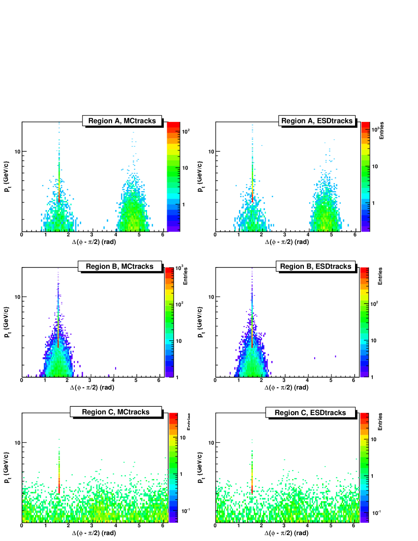
In the Fig. 9 we show for the different regions of the thrust map, a two dimensional distribution: $p_{t}$ vs. $\Delta\phi$ for the associated particles.

The table 2 shows a summary of the analyzed events.

Event	MCtracks	ESDtracks	Efficiency	$1-T$ ( $\tau$ ) cuts	$R$ cuts
With $T$	28920	24960	$86\%$	no	no
Dijet	1503	1316	67 $\%$	$\tau\leq 0.03$	$R\leq 0.35$
Monojet	8903	8329	79 $\%$	$\tau\leq 0.03$	$R\geq 0.9$
Mercedes	523	439	62 $\%$	$\tau\geq 0.25$	$R\leq 0.4$

Table 2: Number of events with particular topologies in the analyzed sample of 1.2 million of events.

The efficiency represents the number of reconstructed events of given topology with respect to the generated events.

One observes a $\sim 70\%$ efficiency with respect to the MC. This may indicate that due to reconstruction and $/$ or absorption of particles one relocates events in other parts of the thrust map as shown in Figs. 5-6.

Note that, out of the 1200000 events only $2.4\%$ (with given $T$ ) of them pass the cuts imposed (at least 1 particle with $p_{t}\geq 3$ GeV/c and $|\eta^{leading}|\leq 0.5$ ). The dijets in acceptance reach about $\sim 0.125\%$ of the total, and about $0.04\%$ belong to mercedes event types. About $37.8\%$ of the accepted events belong to clearly identifiable categories, while the others correspond to events with multi-jets closer to the leading jet.

In the next section we will study each one of the topologies selected. That study includes a visualization of the events through the use of the tools of AliRoot.⁵⁵5AliRoot is the name of ALICE Off-line framework for simulation, reconstruction and analysis. It uses the ROOT system as a foundation on which the framework and all applications are built.

4.1 Dijets and monojets

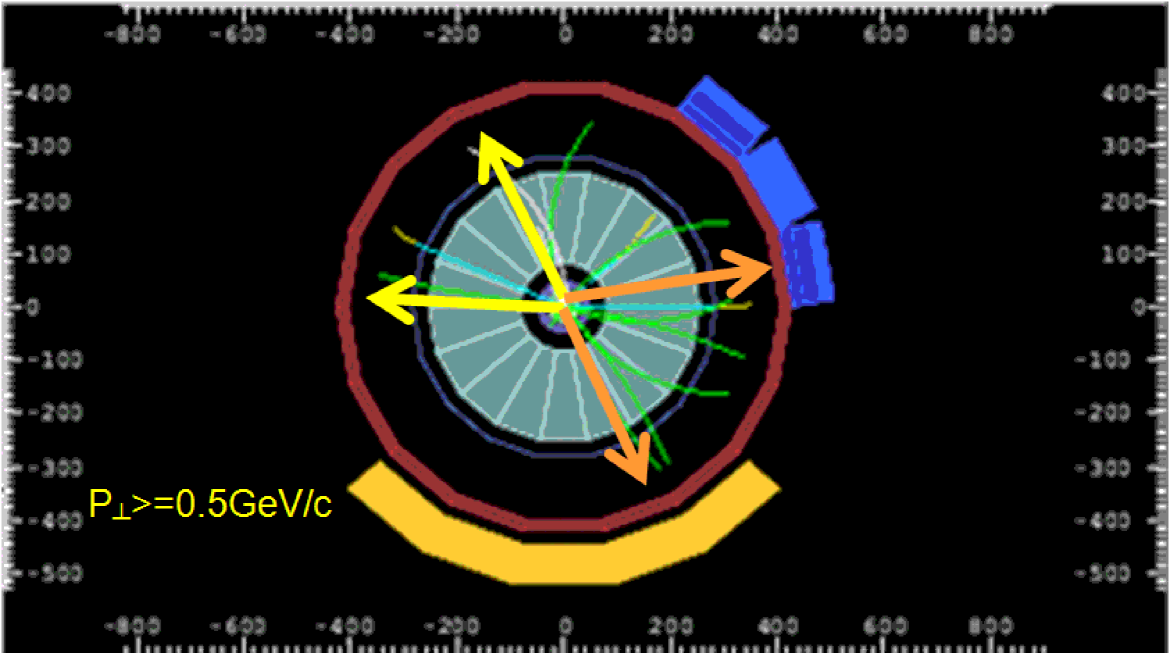
In the present section we are investigating the $p_{t}$ spectra and the multiplicities of the jets in various configurations. As a first step we turn to the visualization tool of events in ALICE. We selected events located in the region A and scanned them. Due to their small $R$ values, they should be inside the acceptance. Fig. 10 shows the visualization of one of them. This particular event has $R=0.00132$ and $1-T=0.0000896$ . The lines are primary monte carlo tracks with $p_{t}\geq 0.5$ GeV/c. The figure clearly shows the whole event contained inside the TPC.

Looking at more events shows always the same structure in the visualization.

Further we computed the total transverse momenta in each jet (here we used all events of the region A).

In order to do it, we divided the event into two parts: toward and away. The first (near side) contains the leading particle and it is formed by all particles in the interval: $\pi/4$ rad $\leq\Delta\phi\leq$ $3\pi/4$ rad. The away side is formed by particles in the interval: $5\pi/4$ rad $\leq\Delta\phi\leq$ $7\pi/4$ .

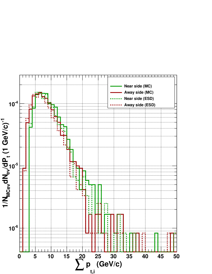
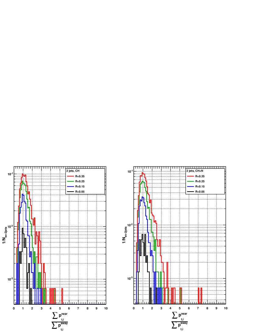
The Fig. 11 shows the distribution of the transverse momentum spectrum of each jet (sum in each azimuthal region of the transverse momentum of all the participants with $p_{t}\geq 0.3$ GeV/c) for generation and reconstruction. The away side distribution is left shifted $\sim 1$ GeV/c with respect to the near side one. This can be understood in terms of the fluctuation of the neutral component of the associated jet and also as effects from the acceptance in the associated jet. In order to illustrate this arguments we plotted the distribution of the ratio: total transverse momenta in the “toward” side over the total transverse momenta in the “away” side for the generation case. The Fig. 12 (right panel) shows the behavior of such distribution (red line). The distribution manifest a clear peak at 1, this fact is in agrement with our assumption about the dijet structure. However the distribution shows many events where the near side jet represent up to 5 times the energy of the away side jet. In this respect the role of the value $R$ is important, because as you can see the width of the distribution decreases as the $R$ interval is decreased. The same analysis can be performed including the neutral component (left panel). The away side jets with a low transverse momentum correspond to events where the away jet is not completely contained.

If you refer to Appendix A of this note, you can convince about ESA allows rejecting events that some jet finders as JETAN could reconstruct as a perfect di-jet, although part of the jet stays out of the acceptance.

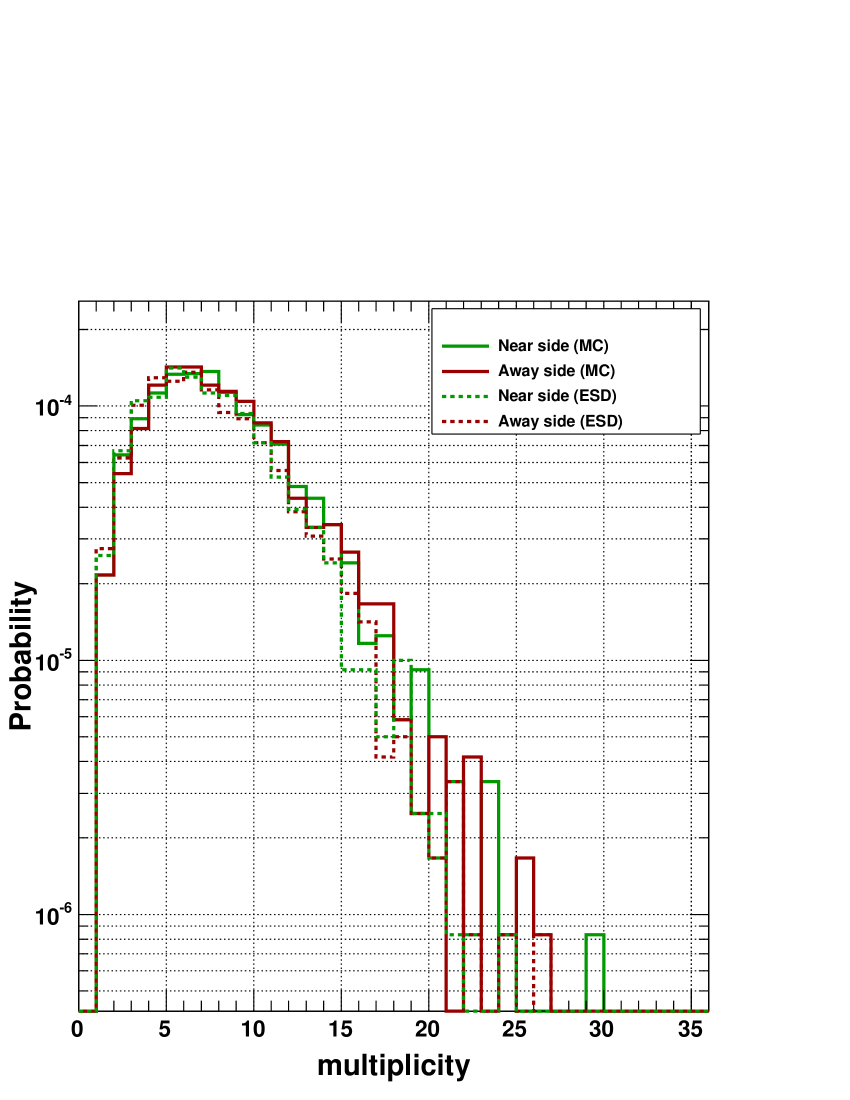
We checked also the multiplicity distributions for the dijets events. In the Fig. 13, we show the multiplicity distribution for the away and toward sides.

A mono-jet event taken from region B of the ESA map is shown in the Fig. 14.

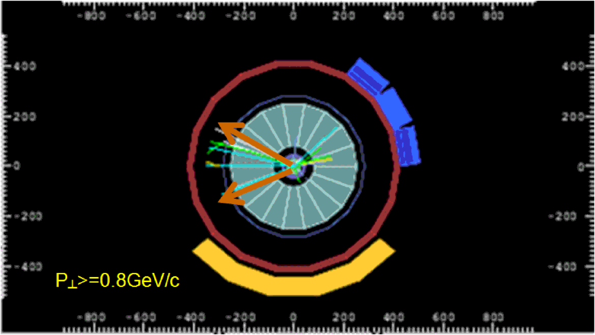
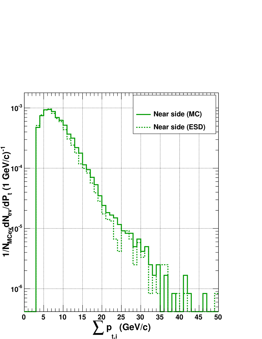
The lines correspond to mctracks with $p_{T}\geq 0.8$ GeV/c. For this event: $1-T=0.00216$ and $R=0.99874$ . Again, by counting primary charged particles within the azimuthal range: $\pi/4$ rad $\leq\Delta\phi\leq$ $3\pi/4$ rad, we estimate the total transverse momentum of the jet. In the Fig. 15, is the distribution of the total transverse momenta for events of region B. Note that the peak of this distribution is at $\sim 6$ GeV/c, in the case of di-jet events this peak is also located at $\sim 6$ GeV/c.

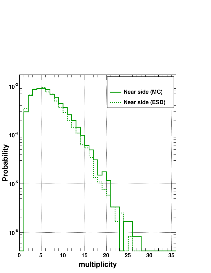
The multiplicity distribution for mono-jet events is in Fig. 16.

The conclusion of this part of the analysis is, that according with the results of the visualization and the behavior of the multiplicity and transverse momentum spectra ESA works fine for discriminating the di-jet events from the mono-jet ones. Using the event shape analysis the signals can be cleaned in order to improve the jet studies.

4.2 Three-jet events

The green distributions of the Fig. 8 allows to observe a double hump structure in the away side of the azimuthal distribution. They look like if the three particles with the highest $p_{t}$ in each event were distributed in the transverse plane according to: the leading particle at $\pi/2$ radians, and the others at: $7\pi/6$ radians and $11\pi/6$ radians, respectively.

There are many configurations of isotropic distributions that could lead to high $1-T$ values, however the scans of the events as shown in Fig. 17 for a typical event result in a clear three jets configurations. A small contribution from events with more than 3 jets can be found.

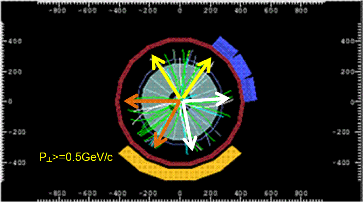
It is important to say that this class of events occurs completely inside the acceptance of our detector, we have to remind that this is controlled by the term $R$ . For example, if we increase the range of $R$ , the azimuthal distribution in the away side shows a shift of the two peaks because the calculation of the variables use incomplete information of the event.

In order to see the conservation of the transverse momentum in this class of events, we divided the azimuth into three regions:

Near side: formed by particles in the azimuthal range: $\pi/4$ rad $\leq\Delta\phi\leq$ $3\pi/4$ rad.
Away side: formed by the particles in the remainder of the azimuth.

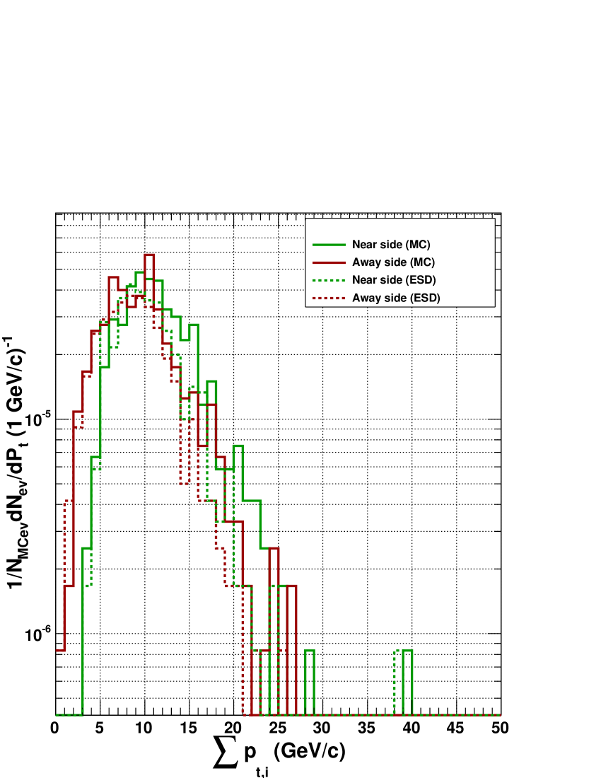
As in the previous cases we have taken into account only primary charged particles with $p_{t}>0.3$ GeV/c. The Fig. 18 shows the transverse momentum of each side. The agreement between both spectra is reasonable in the limits of the statistics.

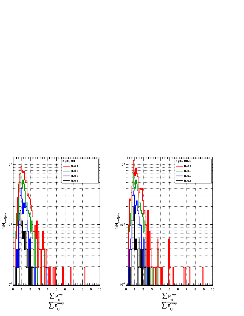
We compute also event by event the ratio of the transverse momenta of the toward jet over the vectorial sum of the away jets as a function of $R$ . The result of this analysis is shown in the Fig. 19. Again these distributions reach their peaks at 1, suggesting the correct transverse momentum conservation.

The events with mercedes topology were found in MB simulation at 10 TeV in the c. m. as well as in MB simulations at 200 GeV [18].

4.3 Multiplicity in the context of ESA.

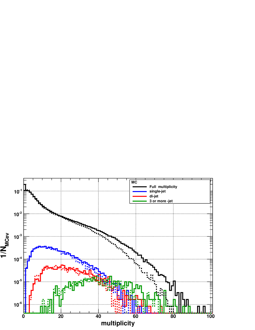
In this section we investigate the multiplicity of each event which we selected. In order to do this task we plotted the multiplicity spectra of the full sample (1 200 000 events), and we compared it with the multiplicities of the events with a given thrust value. The multiplicity is the number of primary charged particles in the acceptance $|\eta|\leq 1$ with $p_{t}>0.3$ GeV/c. As we can see in the plots of the Fig. 20, the conditions which we demanded to each event reduces the number of low multiplicity events. The events with are not related with any of the classes we studied belong to multi-jet events, and also are of high multiplicity. We observe that the mercedes events are generally of large multiplicities.

5 Bulk analysis

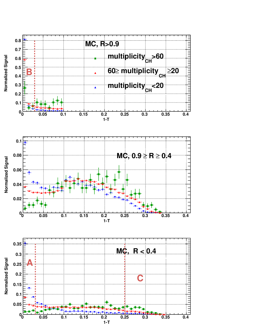
The analysis of the event shape space projected on the $1-T$ offers also interesting results. Without detailed analysis of tje jet components one may directly compare with the different generators. In the following we present the results of each analysis for the generators: Pythia and Phojet. Another interesting question is what happens with the events which thrust and recoil values are outside of the regions A, B and C. In the figure 21 there is the $1-T$ normalized spectrum for different multiplicity bins. Three histograms are shown, the upper one corresponds to the cut $R<0.9$ , the middle: $0.9\geq R\geq 0.4$ ; and finally the events with $R<0.4$ appears in the bottom one. It is clear that the distributions are quite different in the cases $R>0.9$ and $R\leq 0.4$ . In the last one the probability of finding a high multiplicity mercedes event is bigger than the probability of finding a low multiplicity event with mercedes topology. For events of region A, the maximum of the distribution is attained for the lowest multiplicity events. Note also, that in the middle $R$ region (unexplored yet); the spectrums associated to different multiplicity bins are quite similar in their shape.

5.1 Comparison between Pythia and Phojet in the context of ESA

The Monte Carlo generators Phojet [19] and Pythia [20] use both LO QCD matrix elements for the hard scattering sub-processes. Initial and final state parton radiation and the string fragmentation model are included as implemented in the JETSET program [21]. The two Monte Carlo generators differ in the treatment of multiple interactions and the transition from hard to soft processes at low transverse parton momentum. The hard parton-parton cross-section diverges towards low transverse momenta and therefore needs a regularization to normalize to the measured total cross-section.

Hadronic collisions at high energies involve the production of particles with low transverse momenta, the so-called soft multi-particle production. The theoretical tools available at present are not sufficient to understand this feature from QCD alone and phenomenological models are typically applied in addition to perturbative QCD. The Dual Parton Model (DPM) [22] is such a phenomenological model and its fundamental ideas are presently the basis of many of the Monte Carlo implementations of soft interactions.

The Monte Carlo event generator Phojet can be used to simulate hadronic multi-particle production at high energies for hadron-hadron, photon-hadron, and photon-photon interactions with energies greater than 5 GeV. It implements the DPM as a two-component model using Reggeon theory for soft and leading order pQCD for hard interactions. Each Phojet collision includes multiple hard and multiple soft pomeron exchanges, as well as initial and final state radiation. In Phojet pQCD interactions are referred to as hard Pomeron exchange. In addition to the model features as described in detail in [19], the version 1.12 incorporates a model for high-mass diffraction dissociation including multiple jet production and recursive insertions of enhanced pomeron graphs (triple-, loop- and double-pomeron graphs).

So, Phojet provides an alternative to Pythia for the study of processes that cannot be calculated with pQCD, such as minimum bias events (events with high cross section and low transverse momentum) and the underlying event activity in events with a high transverse momentum parton-parton collision.

5.2 Implementation of ESA

The Pythia and Phojet events used are part of the standard simulations in ALICE. The samples are staged on alicecaf and they correspond to proton-proton collisions at 10 TeV in the c. m., minimum bias, magnetic field of 0.5 T. This analysis was done using 200 000 events in each sample.

The Fig. 22 shows the comparison between the normalized spectrum $1-T$ for the samples generated with Pythia and Phojet. Three different regions in $R$ are explored: the first one: populated by single-jet events ( $R>0.9$ ). The second is the intermediate $R$ zone ( $0.4\leq R\leq 0.9$ ). And finally the zone where there are di-jet and three-jet events ( $R<0.4$ ).

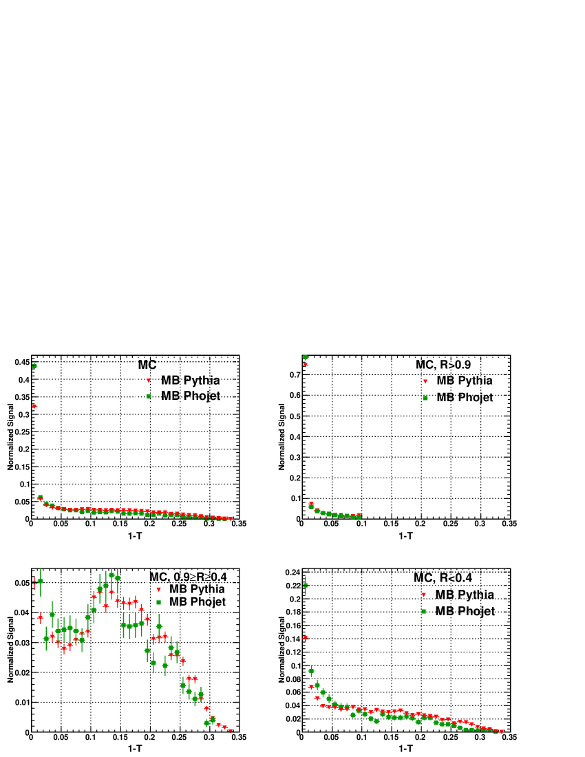
Note that in agrement with the discussion of the previous section, we can observe in the region of the highest values of $R$ and $1-T$ a more copious presence of mono-jet events in the simulations generated by Phojet than in the case of Pythia ones. The same situation appear in the case of di-jet events. Also, note that the particles generated by Pythia look distributed in a way more isotropic compared to the Phojet sample. For the more isotropic topologies and especially the mercedes events the production with Pythia is more copious than with Phojet.

6 Conclusions

In the present note we have demonstrated the applicability of the Event Structure Analysis in the case of measurements of charged particle tracks in a detector of limited acceptance like ALICE. The phase space in recoil and thrust variables offers a wide variety of possible uses:

Selection of well characterized events like monojets, dijets and three jets ones. ESA is in that instance not a replacement for any kind of jet finder but more of a preselection that can be then studied with jet algorithms. As we report the number of “clean” dijets for instance is minute in comparison with the total sample. The use of conventional jet finding algorithm in events with many jets as is the case at LHC leads inexorably to the use of cuts that are sometimes leading to results difficult to interpret.
Bulk comparison of the event characteristics with existing models. Since in the majority of cases we are confronted with multijets events we believe useful to establish a way to compare model predictions with projection on the sphericity axis of events belonging to different recoil and/or multiplicity intervals.
Last but not least any deviation of the present predictions of generator would lead to a rapid detection of events located in an “odd” region of the $R$ vs. $(1-T)$ phase space.

We have presented the discrimination power of ESA for specific topologies: dijets events, monojets and three jet topologies. According to the results presented, the ESA may be of use in the physics analysis starting with the first data since with a sample of 400000 events of minimum bias events, there are many events with the topologies which we discussed.

7 Acknowledgement

The authors would like to thank Dr. J-P Revol for suggesting the present work and for judicious comments to the results; the discussions with E. Cuautle and I. Dominguez were of help in elucidating some aspects of the analysis presented here. One of us (A.O.) would like to acknowledge the HELEN fellowships which greatly helped in getting full proficiency in the use of the ALIROOT framework. The work was performed under the projet IN115808 and Conacyt P79764-F.

Appendix A Appendix

A.1 About the usefulness of ESA in combination with JETAN

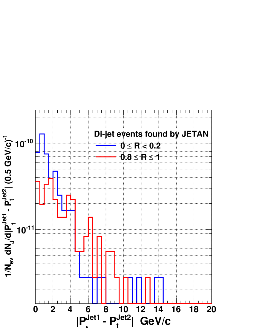
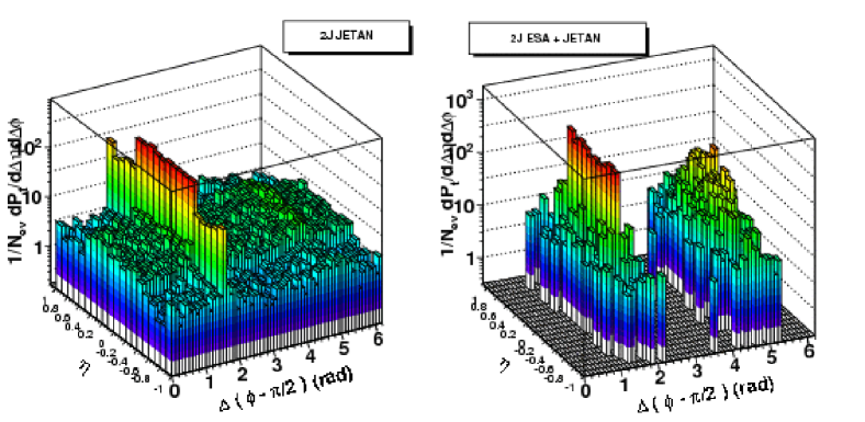
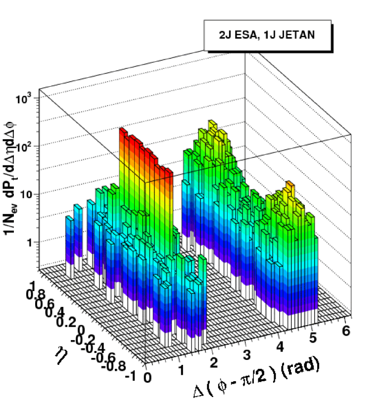
The number of jet to be encountered in pp collisions at the LHC will be very large. In the general case we will find many overlapping jet cones as is shown in Fig.1. On the other hand the small acceptance for jets causes that many jets are only partially in the acceptance. We illustrate that with Fig.23 where we present the ratio of the difference of the total transverse momenta found for events identified by JETAN⁶⁶6JETAN is a module of AliRoot which includes different jet finders. In this analysis we used the UA1 jet finder algorithm which is based on a cone type[23]. The cut in the transverse momentum of the particles which we included is: $p_{t}\geq 1.5$ in the cone radius: $\sqrt{(\Delta\phi)^{2}+(\Delta\eta)^{2}}=0.7$ . And the minimum transverse energy of the jets: 1.5 GeV. as dijets but belonging in the ESA analysis to two different slices in R. For the lowest one $R<0.2$ we see that the difference of momenta is generally small while for the slice of the highest R the difference is markedly broader. We therefore believe that ESA apart from other virtues for the analysis of bulk properties of the events has a very important task to play in the identification of specific topologies. The subsequent comparison of these identified topologies with any kind of jet finder allows in our mind to study “well cleaned” samples without resorting to different cuts as is usual in the use of the jet finders. To illustrate our point of view we show two figures: Fig.24 the distribution of particles in the eta phi acceptance of ALICE using events identified as dijets by JETAN, and on the right side the distribution obtained for events identified as dijets by JETAN applied to ESA dijet events. A completely clean separation between the near and far side jets is visible. However, applying JETAN to the ESA dijet sample we found that a number of events were identified in the present use of ESA as monojet events. The reason is clear from the eta phi distribution in Fig.25 where we plot the “monojet” events found by JETAN. The reason is simple - in ESA we did not limit the eta range for the leading particle of the “away” jet. Hence a part of the events are de facto encountered in the edges of the eta acceptance. The detailed study of these distribution will be pursued.

References

[1] G. Hanson et al., Phys. Rev. Lett. 35 (1975) 1609.
[2] (MARK-J Collaboration), Phys. Rev. Lett. 43, 830 (1979).
[3] (PLUTO Collaboration), Phys. Rev. Lett. B86, 418 (1979).
[4] (TASSO Collaboration), Phys. Rev. Lett. B86, 243 (1979).
[5] (JADE Collaboration), Phys. Rev. Lett. B91, 142 (1980).
[6] S. Bethke, Nucl. Phys. 121 (Proc. Suppl.) (2003) 74.
[7] S. Kluth, et al. Eur. Phys. J. C 21 (2001) 199.
[8] P. Abreu, et al. (DELPHI Collaboration), Z. Physik C 73 (1996) 11.
[9] G. Marchesini et al., Comput. Phys. Commun. 67 (1992) 465.
[10] G. Marchesini et al., Comput. Phys. Commun. 67 (1992) 465.
[11] T. Sjöstrand, Comput. Phys. Commun. 82 (1994) 74.
[12] A. Banfi et. al., Fermilab-PUB-04-117-T (hep-ph/0407287).
[13] J. F. Grosse-Oetringhaus and C. Ekman, Measuring the pseudorapidity density of primary charged particles using the TPC, ALICE-INT-2007-005.
[14] (ALICE Collaboration) J. Phys. G: Nucl. Part. Phys. 32 (2006) 12952040
[15] A. Adare, et al. (PHENIX Collaboration), Phys. Rev. C 78, 014901 (2008).
[16] Y. L. Dokshitzer, G. Marchesini and B. R. Webber, Nucl. Phys. B 469 (1996) 93.
[17] S. Catani, L. Trentadue, G. Turnock and B. R. Webber, Nucl. Phys. B 407 (1993) 3-
[18] A. Ayala et al., Fine structure in the azimuthal transverse momentum correlations at $\sqrt{s_{NN}}=200$ GeV using the event shape analysis , (2009) [arXiv:hep-ph /0902.0074], to be published in Eur. Phys. J. C.
[19] R. Engel, Ph.D. thesis, Hadronic interactions of photons at high energies, Universität Siegen, 1997.
[20] T. Sjöstrand, Comput. Phys. Commun. 82 (1994) 74.
[21] T. Sjöstrand, M. Bengtsson, Comput. Phys. Commun. 43 (1987) 367.
[22] A. Capella et al. Phys. Rep. 236 (1994) 225
[23] (UA1 Collaboration), Arnison et al., Phys. Lett. 132B, 214 (1983).