Neural-estimator for the surface emission rate of atmospheric gases

Abstract

The emission rate of minority atmospheric gases is inferred by a new approach based on neural networks. The new network applied is the multi-layer perceptron with backpropagation algorithm for learning. The identification of these surface fluxes is an inverse problem. A comparison between the new neural-inversion and regularized inverse solutions is performed. The results obtained from the neural networks are significantly better. In addition, the inversion with the neural networks is faster than regularized approaches, after training.

1 Introduction

The enhancing of the concentration of greenhouse effect gases is a central issue nowadays, meanly regarding the most important anthropogenic gases, such as methane ($CH_{4}$) and carbon dioxide ($CO_{2}$). Despite the ratification of the Kyoto Protocol, the forecast is that the releases of $CO_{2}$ and $CH_{4}$ in the atmosphere continue to increase in next decade [16].

One mandatory strategy is to monitoring the concentration of these gases in the atmosphere. However, in order to understand the bio-geochemical cycle of these gases, it is necessary to estimate the surface emission rates. One procedure for this is to employ inverse problem methodology.

The method of inverse problem is an efficient way to scientifically estimate the intensity of pollution sources. Various inverse problem methods are being investigated by the international scientific community [8, 25, 26]. In order to deal with the ill-posed characteristic of inverse problems, regularized solutions [4, 28] and also regularized iterative solutions [1, 5] have been proposed. More recently, artificial neural networks are also employed to solve inverse problems [15, 31, 27]. The pollutant source identification is an inverse problem, and neural networks have been applied for identifying the emission intensity of point sources [17, 20, 12, 21, 30].

In this paper, a new approach using multilayer perceptron artificial neural network (MLP-ANN) is employed to estimate the rate of surface emission of a pollutant. The input for the ANN is the gas concentration measured on a set of points. The methodology is tested using synthetic experimental data, obtained by running an atmospheric pollutant dispersion model: LAMBDA [10, 11]. The Lambda model is a Lagrangian model.

Finally, the surface rate estimated with MLP-ANN is compared with regularized inversion by maximum entropy principle. In the latter method, the inverse problem is formulated as an optimization problem that could be solved using a deterministic or a stochastic optimization procedure.

2 Forward Model

The Lagrangian particle model LAMBDA was developed to study the transport process and pollutants diffusion, starting from the Brownian random walk modeling [11, 9]. In the LAMBDA code, full-uncoupled particle movements are assumed. Therefore, each particle trajectory can be described by the generalized three dimensional form of the Langevin equation for velocity [29]:

$$du_{i}=a_{i}\left(\textbf{x},\textbf{u},t\right)dt+b_{ij}\left(\textbf{x},\textbf{u},t\right)dW_{j}(t)$$ (1)

$$d\textbf{x}=\left(\textbf{U}+\textbf{u}\right)dt$$ (2)

where $i,j=1,2,3$, and x is the displacement vector, U is the mean wind velocity vector,u is the Lagrangian velocity vector, $a_{i}\left(\textbf{x},\textbf{u},t\right)$ is a deterministic term and $b_{ij}\left(\textbf{x},\textbf{u},t\right)dW_{j}(t)$ is a stochastic term and the quantity $dW_{j}(t)$ is the incremental Wiener process.

The determinisitc (drift) coefficient $a_{i}\left(\textbf{x},\textbf{u},t\right)$ is computed using a particular solution of the Fokker-Planck equation associated to the Langevin equation. The diffusion coefficient $b_{ij}\left(\textbf{x},\textbf{u},t\right)$ is obtained from the Lagrangian structure function in the inertial subrange $\left(\tau_{K}<<\Delta t<<\tau_{L}\right)$, where $\tau_{K}$ is the Kolmogorov time scale and $\tau_{L}$ is the Lagrangian de-correlation time scale. These parameters can be obtained employingthe Taylor statisitcal theory on turbulence [32].

Backward integration can also be applied. This is just to identify which particle arriving in a sensor-$j$ is coming from a source-$i$.

The drift coefficient, $a_{i}\left(\stackrel{{\scriptstyle\rightarrow}}{{\textbf{x}}},\stackrel{{\scriptstyle\rightarrow}}{{\textbf{u}}},t\right)$, for forward and backward integration is given by

$$a_{i}P_{E}=c_{v}\left[\frac{\partial\left(B_{i,j}P_{E}\right)}{\partial\textbf{u}_{j}}+\phi_{i}\left(\textbf{x},\textbf{u},t\right)\right]$$ (3)

with

$$\frac{\partial\phi_{i}}{\partial\textbf{u}_{i}}=-\frac{\partial P_{E}}{\partial t}-\frac{\partial\left(\textbf{u}_{i}P_{E}\right)}{\partial\textbf{x}_{i}}$$ (4)

and

$$\phi_{i}\rightarrow 0\textit{when}\stackrel{{\scriptstyle\rightarrow}}{{\textbf{u}}}\rightarrow\infty$$ (5)

where $c_{v}=1$ for forward integration and $c_{v}=-1$ for backward integration, $P_{E}=P\left(\stackrel{{\scriptstyle\rightarrow}}{{\textbf{x}}},\stackrel{{\scriptstyle\rightarrow}}{{\textbf{u}}},t\right)$ is the non-conditional PDF of the Eurelian celocity fluctuations, and $B_{i,j}=\frac{1}{2}b_{i,k}b_{j,k}$.

Of course, for backward integration, the time considered is: $t^{\prime}=-t$, and velocity $\textbf{U}^{\prime}=-\textbf{U}$, being U the mean wind speed. The horizontal PDFs are considered Gaussians, and for the vertical coordinate the truncated Gram-Charlier type-C of third order is employed [33].

The diffusion coeffiecients, $b_{ij}\left(\textbf{x},\textbf{u},t\right)$, for both forward and backward integration is given by

$$b_{ij}=\delta_{ij}\left[2\frac{\sigma^{2}_{i}}{\tau_{Li}}\right]^{1/2}$$ (6)

where $\delta_{ij}$ is teh Kronecker delta, $\sigma^{2}_{i}$ and $\tau_{Li}$ are velocity variance at each component and the Lagrangian time scale [32], respectively. With the coordinates and the mass of each particle, the concentration is computed - see equations (5) and (6).

The inverse problem here is to identify the source term $S(t)$. As mentioned, a source-receptor approach is employed for reducing the computer time, instead of running the direct model (equation 2) for each iteration. This approach displays an explicit relation between the pollutant concentration of the i-th receptor related the j-th sourcers:

$$C_{i}=\sum^{N_{S}}_{j=1}M_{ij}S_{j}$$ (7)

where the matrix $M_{ij}$ is the transition matrix, and matrix entry given by

$$M_{ij}=\left\{\begin{array}[]{ll}\left(\frac{V_{S,j}}{V_{R,i}}\right)\left(\frac{\Delta t}{N_{S,j}}\right)N_{R,i,j}\left(\textit{forward}\right)\\ \left(\frac{\Delta t}{N_{S,j}}\right)N_{S,i,j}\left(\textit{backward}\right)\end{array}\right.$$ (10)

where $V_{R},i$ and $V_{S,j}$ are the volumr for the i-th receptor and j-th source, respectively; $N_{S,j}$ and $N_{R,i}$ are the number of particle realised by the j-th source and i-th sensor, respectively; $N_{R,i,j}$ and $N_{S,i,j}$ are the number of particle released by the j-th source and detected by the i-th receptor.

3 Inverse Method: Neural Network

An artificial neural network (ANN) is an interconnected group of artificial neurons, elements of networks that uses a mathematical or computational model for information processing based on a connectionist approach to computation. Inputs and outputs to a neuron consist of values $\left(x_{1},x_{2},\ldots,x_{n}\right)$ and $\left(y_{1},y_{2},\ldots,y_{n}\right)$. The neuron computes the weighted sum of its inputs, adding a bias, and the result is an argument for a non-linear activation function. The MLP is composed of multiple processing units called artificial neurons (or nodes) arranged in several different layers [2]. The configuration of the best MLP model includes choosing the number of layers (typically, it requires at least three: input, hidden, and output), the number of neurons in hidden layer (how many units should be in the input and output layers is defined by the problem), the activation function, and the learning algorithm. After the proper architecture of the MLP has been established, all the training cases are run through the network. In each neuron a linear combination of the weighted inputs (including a bias) is computed, summed and transformed using a transfer function (linear or nonlinear). The value obtained is passed on as an input to the neurons in the subsequent layer until a value is computed in neurons of the output layer. The output values are compared with the target values. The difference between the output and target is calculated for each output neuron using a certain error function in order to give the prediction error made by the network. Then, the training algorithm is used to adjust the network’s weights and thresholds in order to minimize this error. Because a target value is compared to the output value, the learning process is called supervised [14]. In this study a linear transfer function was used in input neurons, and the log-sigmoid function for the neurons located in hidden and output layers. The error function was the sum-squared error, where the individual errors of output units on each case were squared and summed together. The networks were trained using the back-propagation algorithm [2]. The correctionof the weights $\Delta w$ was calculated according to the following formula: $\Delta w_{ij}=\eta\delta_{j}o_{i}+\alpha\Delta w^{\left(old\right)}_{ji}$, in wich j is the index of the neuron in the current layer, the neuron in the upper layer is indexed by i and its output by $o_{i}$, and the local error gradient is denoted by $\delta_{j}$. There are two constants in this formula - the learning rate $\eta$, wich determines to what extent the weights should be modified, and the momentum coefficient $\alpha$, which decides to what degree this previous adjustment is to be considered so as to prevent any sudden changes in the direction in which corrections are made. The learning rate $\eta$ and momentum $\alpha$ were set to 0.1 and 0.5, respectively. They can be used to model complex relationships between inputs and outputs or to find patterns in data. In this paper, we used the neural network MLP feedforward backpropagation network is the multilayer perceptron (MLP) with backpropagation learning.

Regardless their type or use, all neural networks have three stages in their application: the learning, the activation and the generalization steps. It is in the learning step that the weights and bias corresponding to each connection are adjusted to some reference examples (the input). In the activation phase, the output is obtained based on the weights and bias computed in the learning phase [14]. The transfer function selected was a tan-sigmoid transfer function for the hidden layers and linear transfer function for the output layer. The experimental data used here in the learning step were simulated adding a random perturbation to the exact solution for forward problem (LAMBDA):

$$\widehat{I}=I_{exact}\left(1+\sigma\mu\right)$$ (11)

where $\sigma$ is the noise standard deviation and $\mu$ is a random variable taken from a Gaussian distribution with zero mean and unitary variance. In all simulations we used $\delta=0.05$ and $\delta=0.10$.

Overall, more than fifty pairs of rates of emission of pollutants and their concentrations are necessary for the process of inversion. Similar data sets were used for the stages of activation and the general ANN.

4 Results

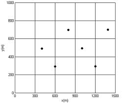
Figure 1: Computational domain divided into 25 subdomains.

The area of the numerical experiment used is the same employed by Roberti (2005) [22] and Luz (2007) [18]. The domain is divided into 25 sub-domains, where each cell has the size: 300 m (width) x 200 m (length) - volume of each cell is 60.000.000 $m^{3}$ (height = 1000 m) [22]. Figure 1 shows the different subdomains of emissions of contaminants. In this figure, there are sensors, where their positions are represented by $\bullet$ in the area of study.

Six sensors are used inside the domain, and the sensor size is a small volume: 0.1 m x 0.1 m x 0.1 m, positioned at a height of 10 meters, installed in the area, according to Table Table 1.

Table 2 shows the meteorological data used by the LAMBDA model to simulate the dispersion of particles, taken from the Copenhagen experiment [22, 10]. Meteorological data are speeds and direction averages of wind, measured at three levels, for five different time periods measured on 19/10/1978 [22].

The results obtained with noiseless data are in excellent agreement with the true model. The MLP network produced good estimation of the rate of emission of pollutants compared to the Quasi-Newton method [22] and Particle Swarm Optimization (PSO) [18]. The best results for noisy data were obtained for the MLP network with 15 and 30 neurons in hidden layer and $\delta=0.05$.

In order to analyze the performance of the ANNs for the estimation of the rate of gas emission, two experiments were performed. In the first experiment 5% of white Gaussian noise ($\delta=0.05$) was added to the synthetic experimental data. In the second one, 10% of noise is used to simulate the real experimental data. All ANNs were trained with two hidden layers, varying the number of hidden neurons and the database training. Several tests were carried out to reach in a good neural network architecture. For all configurations, two hidden layers were considered: (a) ANN-1: 6 and 12, (b) ANN-2: 7 and 8, (c) ANN-3: 15 and 30 neurons in hidden layers. The ANN-3 obtained the best result compared with the model true. Figure 2 and Figure 3, the topology of the RNA is represented as: $x_{1}:x_{2}:x_{3}:x_{4}$ where $x_{1}$: number of neurons in input layer, $x_{2}$: number of neurons in the 1st hidden layer, $x_{3}$: number of neurons in the 2nd hidden layer and $x_{4}$: Number of neurons in output layer.

The training phase was carried out until a maximum number of iterations were reached. Table 3 shows the exact results (LAMBDA), the results obtained with regularized inversion (the optimization problem solved by quasi-Newton (Q-N, deterministic) [22] and particle swarm optimization (PSO, stochastic) [18] schemes), and the results obtained with ANN for $\delta=0.05$. The Table 4 shows the same results, but considering $\delta=0.10$.

Figures Figure 2 and Figure 3 shows the results of the generalization tests in comparison with the true model.

5 Conclusion

The problem for identifying the minority gas emission rate for the system ground-atmosphere is an important issue for the bio-geochemical cycle, and it has being intensively investigated. This inverse problem has been solved using regularized solutions [25], Bayes estimation [8, 13], and variational methods [7] (this is approach started from the data assimilation studies).

Our previous studies were initiated using generalized least square scheme, with entropic regularization [22, 23, 18, 19] (for the use of maximum entropy principle on this issue, see also [3, 6]).

ANNs were used as effective tool for solving the inverse problem of estimation of the rate of gas surface emission. The obtained reconstructions with the MLP showed to be better than the obtained with regularization methods [22, 18]. Another advantage of the use of neural network is, after the training phase, the reconstruction algorithm is faster than the regularized inversion methods. Neural inversion is unique scheme that does not need a solution of the associated forward problem.

In practice, operational inversion algorithms reduce the risk of being trapped in local minima by starting the iterative search process from an initial guess solution that is sufficiently close to the true profile. However, the dependence of the final solution on a good choice of the initial guess represents a fundamental weakness of such algorithms, particularly in regions where less a priori information is available [17]. ANN approaches can relax this constraint incorporating more data in the dataset during the learning phase.

The ANNs can be inaccurate if they are used to extrapolate to cases outside the training domain. However the use of ANN techniques can provide good solutions when the training phase encompasses the domain of the potential solutions to the real problem.

Table 1: Position of the sensors in the area.

Sensor	Position x (m)	Position y (m)
1	400	500
2	600	300
3	800	700
4	1000	500
5	1200	300
6	1400	700

Table 2: Meteorological data used in the experiment Copenhagen.

Time	Speed $\overline{U}$ (m/s)			Direction $\overline{U}$ ( )
(h:m)	10 m	120 m	200 m	10 m	120 m	200 m
12:05	2,6	5,7	5,7	290	310	310
12:15	2,6	5,1	5,7	300	310	310
12:25	2,1	4,6	5,1	280	310	320
12:35	2,1	4,6	5,1	280	310	320
12:45	2,6	5,1	5,7	290	310	310

Table 3: Results of estimation of the rate o gas emission ($gm^{-3}s^{-1}$), for noise level $\sigma=0.05$.

cell	Exact	Q-N ($gm^{-3}s^{-1}$)	PSO ($gm^{-3}s^{-1}$)	ANN 6:6:12:12	ANN 6:15:30:12
	($gm^{-3}s^{-1}$)	(Roberti, 2005)	(Luz, 2007)	($gm^{-3}s^{-1}$)	($gm^{-3}s^{-1}$)
$A_{2}$	10	9,82	09,34	09,92	09,79
$A_{3}$	10	9,63	10,07	09,83	09,74
$A_{4}$	10	11,26	11,26	09,86	04,81
$A_{7}$	10	8,76	10,95	09,82	09,80
$A_{8}$	10	11,06	10,93	09,71	09,73
$A_{9}$	10	15,51	14,99	09,71	09,79
$A_{12}$	20	20,12	20,79	20,94	20,61
$A_{13}$	20	19,25	19,83	20,81	20,61
$A_{14}$	20	11,52	13,06	20,93	20,60
$A_{17}$	20	17,88	18,72	20,94	20,60
$A_{18}$	20	23,82	22,76	20,96	20,61
$A_{19}$	20	23,44	22,47	20,77	20,59

Table 4: Results of estimation of the rate o gas emission ($gm^{-3}s^{-1}$), for noise level $\sigma=0.10$.

cell	Exact	Q-N ($gm^{-3}s^{-1}$)	PSO ($gm^{-3}s^{-1}$)	ANN 6:6:12:12	ANN 6:15:30:12
	($gm^{-3}s^{-1}$)	(Roberti, 2005)	(Luz, 2007)	($gm^{-3}s^{-1}$)	($gm^{-3}s^{-1}$)
$A_{2}$	10	8,97	09,83	10,33	10,11
$A_{3}$	10	9,97	10,40	10,11	10,11
$A_{4}$	10	12,52	10,79	10,12	10,20
$A_{7}$	10	7,98	10,50	10,27	10,20
$A_{8}$	10	10,14	12,06	10,24	10,06
$A_{9}$	10	11,56	11,28	10,17	10,17
$A_{12}$	20	13,84	14,56	21,21	20,97
$A_{13}$	20	22,65	22,67	21,28	21,00
$A_{14}$	20	14,14	15,85	21,32	20,95
$A_{17}$	20	19,99	21,56	21,47	20,99
$A_{18}$	20	21,17	20,05	21,47	20,99
$A_{19}$	20	24,90	21,74	21,48	20,96

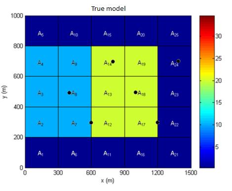
(a)

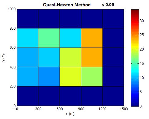
(b)

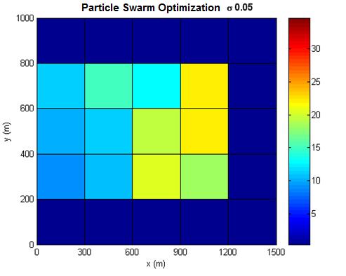
(c)

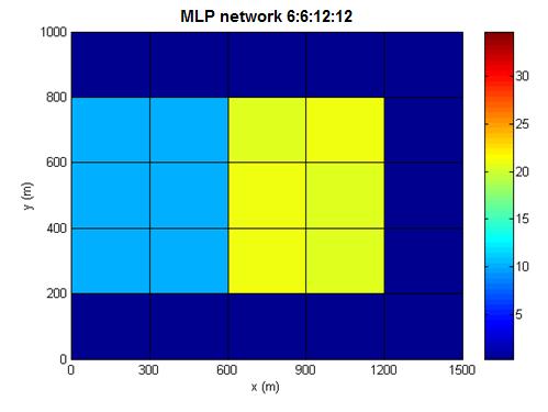
(d)

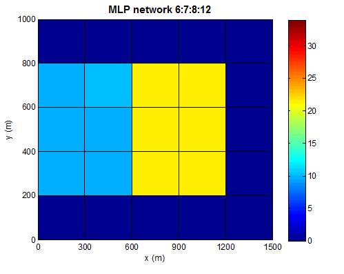
(e)

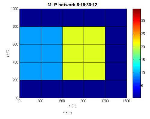
(f)

Figure 2: Generalization results of rate of emission of pollutant (in $gm^{-3}s^{-1}$) for noiseless data using $\sigma=0.05$. (a) True model; (b) Quasi-Newton [22]; (c) PSO [18]; (d)6 and 12 neurons hidden layer; (e) 7 and 8; (f) 15 and 30.

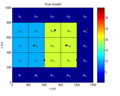
(a)

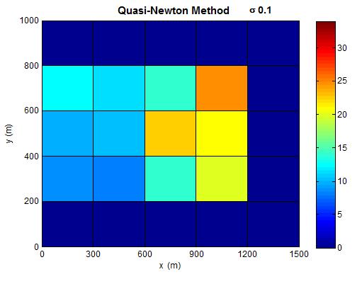
(b)

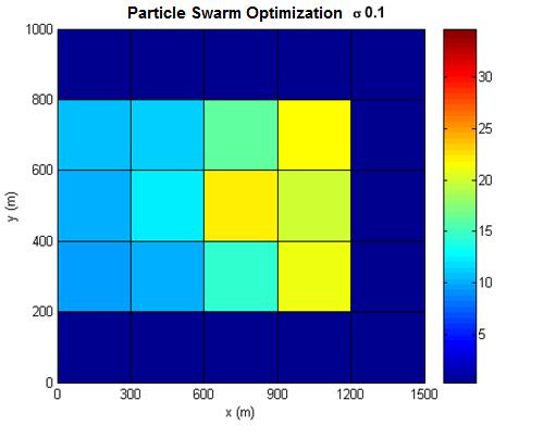
(c)

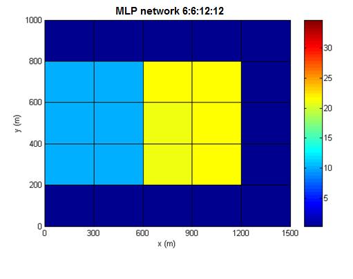
(d)

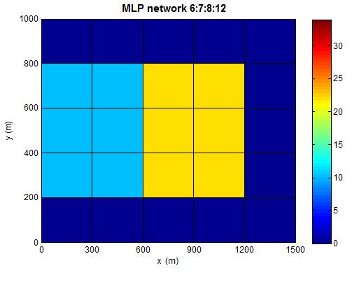
(e)

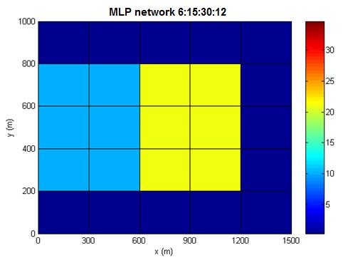
(f)

Figure 3: Generalization results of rate of emission of pollutant (in $gm^{-3}s^{-1}$) for noiseless data using $\sigma=0.10$. (a) True model; (b) Quasi-Newton [22]; (c) PSO [18]; (d)6 and 12 neurons hidden layer; (e) 7 and 8; (f) 15 and 30.

References

- [1] Alifanov, O., 1974. Solution of an inverse problem of heat conduction by iteration methods. Journal of Enginnering Physics, 26(11), 471-476.
- [2] Bishop, C.M., 1995. Neural networks for pattern recognition. Oxford University Press, Oxford.
- [3] Bocquet, M., 2005 Grid resolution dependence in the reconstruction of an atmospheric tracer source, Nonlinear Processes in Geophysics, 12, 219-234.
- [4] Campos Velho, H. F., Ramos, F. M., 1997. Numerical inversion of two-dimensional geoletric conductivity distributions from eletromagnetic ground data. Jorunal of Geophysis, 15 (2), 133-143.
- [5] Chiwiaciwsky, L., Campos Velho, H. F., 2006 Different approaches for the solution of a backward heat conduction problem. Inverse Problems in Engineering, 11(6), 471-494.
- [6] Davoine, X., Bocquet, M., 2007. Inverse modelling-based reconstruction of the Chernobyl source term available for long-range transport, Atmospheric Chemistry and Physics, 7, 1549-1564.
- [7] Elbern, H., Strunk, A.,Schmidt, H.,Talagrand, O., 2007. Emission rate and chemical state estimation by 4-dimensional variational inversion. Atmospheric Chemistry and Physics, 7, 3749-3769.
- [8] Enting, I. G., 2002. Inverse Problems in Atmospheric Constituent Transport. Cambridge: University Press, 392p.
- [9] Ferrero, E., Anfossei, D., 1998b. Comparison of pdfs, closures schemes and turbulence parameterizations in lagrangian stochastic models. International Journal of Environment and Pollution, 9, 384-410.
- [10] Ferrero, E., Anfossi, D., Brusasca, G., 1995. Lagrangian particle model lambda: evaluation against tracer data. International Journal of Environment and Pollution, 5, 360-374.
- [11] Ferrero, E., Anfossi, D., 1998a. Sensitivity analysis of lagrangian stochastic models for CBL with dierent pdf’s and turbulence parameterizations. Air Pollution Modelling and its Applications XII, 673-680.
- [12] Gardner, M.W., Dorling, S.R., 1999. Neural network modelling of hourly and concentrations in urban air in London. Atmospheric Environment 33, 709-719.
- [13] Gimson, N. R., Uliasz, M., 2003 The determination of agricultural methane emissions in New Zealand using inverse modelingtechniques. Atmospheric Environment, 37, 3903-3912.
- [14] Haykin, S., 1999. Neural Networks: A Comprehensive Foundation. [S.l.]: Prentice Hall.
- [15] Hidalgo, H., G mez-Trevin E., 1996. Application of constructive learning algorithms to the inverse problem. IEEE T. Geosci. Remote, 34(1), 874-885.
- [16] IPCC. Climate Change 2007: The Physical Science Basis. Contribution of Working Group I to the Fourth Assessment Report of the Intergovernamental Panel on Climate Change. [S.I.]: Cambridge University Press, 996p.
- [17] Kukkonen, J., and 10 co-authors, 2003. Extensive evaluation of neural network models for the prediction of NO2 andPM 10 concentrations, compared with a deterministic modelling system and measurements in central Helsinki, Atmos. Environ., 37, 4539-4550.
- [18] Luz, E. F. P., 2008. Estima o de fonte de polui o atmosf rica por enxame de part culas. Disserta o (Mestrado) - Instituto Nacional de Pesquisas Espaciais.
- [19] Luz, E. F. P., Campos Velho, H. F., Becceneri, J. C., Roberti, D. R., 2007. Estimating Atmospheric Area Source Strength Through Particle Swarm Optimization, Inverse Problems, Desing and Optimization Symposium IPDO-2007, April 16-18, Miami (FL), USA.
- [20] Lu, H.C., Hsieh, J.C., Chang, T.S., 2006. Prediction of daily maximum ozone concentrations from meteorological conditions using a two-stage neural network. Atmos Res 81:124-139.
- [21] Pelliccioni A., Tirabassi, T. (2006) Air dispersion model and neural network: A new perspective for integrated models in the simulation of complex situations. s.l.: Environmental Modelling & Software, Vol. 21, pp. 539-546.
- [22] Roberti, D. R., 2005. Problemas inversos em f sica da atmosfera. Tese (Doutorado) - Santa Maria: UFSM - Centro de Ci ncias Naturais e Exatas.
- [23] Roberti, D. R., Anfossi, D., Campos Velho, H. F., Degrazia, G. A., 2005. Estimation of Location and Strength of the Pollutant Sources, Ciencia e Natura, 131-134.
- [24] Roberti, D. R., Anfossi, D., Campos Velho, H. F., Degrazia, G. A., 2007. Estimation of emission rate from experimental data. Nuovo Cimento della Societ Italiana di Fisica. C, Geophysics and Space Physics, 30, 177-186.
- [25] Seibert, P., 2000. Inverse modelling of sulfur emissions in europe based on trajectories inverse Methods in Global Biogeochemical Cycles, p. 147-154.
- [26] Sibert P., 2001. Inverse modelling lagrangian particle dispersion model: aplication to point releases over limited time intervals. Air Pollution modeling and its Aplication XIV, p. 381-389.
- [27] Shiguemori, E. H., Campos Velho, H. F., Silva, J. D. S., 2008. Atmospheric Temperature Retrieval from Satellite Data: New Non-extensive Artificial Neural Network Approach. In: Symposium on Applied Computing, 2008, Fortaleza. Proceedings of the 23rd Annual ACM Symposium on Applied Computing 2008. New York : Association for Computing Machinery, Inc, III, 1688-1692.
- [28] Tikhonov, A. N., Arsenin V. Y., 1977. Solutions of ill-posed problems. Winston & Sons, New York.
- [29] Thomson, D. J., 1987. Criteria for selection of stochastic models of particle trajectories in turbulent flows. Journal of Fluid Mechanics, 180, 529-556.
- [30] Wesolowski, M., Suchacz, B., Halkiewicz, J., 2006. The analysis of seasonal air pollution pattern with application of neural networks. Analytical and bioanalytical chemistry, 384(2), 458-467.
- [31] Woodbury, K., 2000. Neural networks and genetic algorithms in the solution of inverse problems. Bulletim of the Braz. Soc. for Comp. Appl. Math. (SBMAC).
- [32] Degrazia, G.A., Anfossi, D., Carvalho, J.C., 2000. Mangia C.; Tirabassi T.; Campos Velho H.F. Turbulence parameterization for PBL dispersion models in all stability conditions, Atmos. Environ. 34,3575-3583.
- [33] Anfossi D., Ferrero E., 1997. Comparison among Empirical Probability Density Functions of the Vertical Velocity in the Surface Layer Based on Higher Order Correlations, Boundary-Layer Meteorol., 82, 193-218.