An analytical framework to describe the orientation of dark matter halos and galaxies within the large-scale structure

Abstract

We provide a set of general tools for studying the alignments of dark matter halos and galaxies with respect to the large scale structure. The statistics of the positioning of these objects is represented by a Probability Distribution Function (PDF) of their Euler angles. The mathematical identities relating this PDF to the alignment of the halo axes with respect to the direction that characterises locally the large scale structure are given. The PDF corresponding to halos located in the shells of the cosmic voids is inferred from previous results. This PDF is used to show how to recover the outcomes found for the alignments of the axes of these halos in simulations. We also explore the orientation of the angular momentum of the halos, both with respect to the halo axes and with respect to the large scale structure. We present an expression which describes well numerical results for the alignment of the angular momentum of the halo with respect to the halo axes for randomly chosen halos. Combining that expression, with the PDF of the halo positioning with respect to the large scale structure we find, in the case of halos in the shells of voids, an alignment of the angular momentum that is opposite to that found in simulations. To solve this issue, we propose a model that relates the orientation of the angular momentum with the halos axes accounting for the orientation of the halo axes with the large scale structure. This model is shown to recover accurately the observed PDF of the halo angular momentum with respect to the void radial direction. This model also predicts a substantial dependence of the intrinsic alignment of the angular momentum on environment. In addition, we give an expression for determining the degradation of the angular momentum intrinsic alignment when observational errors are accounted. This expression is also used to determine the departure of the observed value of the alignment from the initial expectation (as provided by the tidal torque theory) due to the rotation of the angular momentum of the halo with respect to the initial torque. For voids, we find that the strength of the alignment is reduced to half the original value. We discuss how to adapt the void results to other cosmic large scale structures (i.e. filaments, walls, etc).

1 Introduction

Our current galaxy formation paradigm states that galaxies acquire their angular momentum by a mechanism known as tidal torquing (Sciama 1955; Peebles 1969; Doroshkevich 1970; White 1984). In this paradigm, tidal fields generated from the large-scale structure excerpt a torquing on the protogalactic object prior to gravitational collapse. The acquired angular momentum is conserved during collapse and their value will dictate the formation and orientation of the galactic disks. One important consequence of the tidal torquing theory (TTT) is an expected relation between the large-scale structure and the orientation of the angular momentum of the galaxies within it (see a recent review by Schäfer 2009).

From the observational point of view, Navarro et al. (2004) found a notable (with a significance of 92%) excess of edge-on spiral galaxies (for which the orientation of the disk rotation axis may be determined unambiguously) highly inclined relative to the supergalactic plane. Trujillo et al. (2006) perform a measurement of the rotation axes of galaxies situated on the shells of large cosmic voids and found that the angular momentum of these objects tend to be aligned perpendicular to the radial direction of the void with a significance of 99.7% (see also Slosar & White 2009). Lee & Erdogdu (2007) combined a reconstruction of the density tidal shear field from the 2MASS redshift survey with the spin field derived from the Tully galaxy catalogue and found a correlation strength at the 6$\sigma$ significance level.

From the numerical perspective, the orientation of the halos within their large-scale cosmic structure has been investigated by several authors (Bailin & Steinmetz 2005; Patiri et al. 2006; Brunino et al. 2007; Aragón-Calvo et al. 2007; Cuesta et al. 2008). In particular, Patiri et al. (2006) and Brunino et al. (2007) investigated the alignment of dark matter halos within the shells of large cosmic voids and provided evidence that the minor axis of the dark matter halos points preferentially to the centres of the voids. The intermediate and major axis were found to be preferentially oriented perpendicularly to the void direction. In addition, Cuesta et al. (2008) found, with high significance, a preferential alignment between the angular momentum of the halo and the void direction. As for real galaxies, the angular momentum of the halos tend also to be aligned perpendicular to the radial direction of the void.

Although the orientation of the galaxies and halos within the large-scale structure has been identified both observationally and numerically, there has not been any previous quantitative study neither of the relationship between the various kind of alignments already determined, nor of the connection between these alignments and the existing results for the positioning of the angular momentum with respect to the halo axes. In this paper we use and discuss several previous results concerning the alignments of halo axes and angular momentum with respect to their corresponding voids for those halos lying in the shells of the voids. Not all these results are independent, so we intend to establish a convenient set of independent results from which all other results may be obtained. To this end we shall present the needed mathematical identities relating the various kind of alignments that we shall consider, and use them to infer the set of independent results that we shall choose. Then we shall show that, using the appropriate mathematical relationships, all previous results can be derived, thereby proving their consistency. In this way we shall not only present previous results in a compact and ordered fashion, but shall also present results whose form is valid for the alignment with respect to features of the large scale structure other than voids.

In Section 2, we show how to characterise uniquely the statistics of the orientation of the halos in the shells of the voids with respect to their corresponding voids and how the alignments of the various halo axes may be derived from it. In Section 3, we provide a motivated model for the probability distribution for the orientation of the angular momentum of a randomly chosen halo with respect to its axes. Then, through a modification of this model, we obtain a model for the alignment of the angular momentum with respect to the halo axis for a halo in the neighbourhood of a void (or, in general, within a large scale tidal field). Using this model along with the statistics for the orientation of the halo with respect to the void we obtain the probability distribution for the alignment of the angular momentum with the radial direction of the void. Then, comparing this distribution with that found in simulations, we calibrate that model, inferring a very substantial dependence of the alignment of the angular momentum with respect to the halo axes on the environment. Finally, in Section 4, we discuss the relationship between the alignment of the angular momentum of the halo at the moment of turn around and at present, and how any uncertainty in the determination of the angle of the rotation axis of galaxies with respect to the radial vector joining the centre of the corresponding void with the galaxy diminishes the strength of the alignment. A discussion and a summary of conclusions are given in Sec. 5.

2 Alignments of halo axes with respect to the void radial direction

We shall first consider the alignments of the three halo axes with respect to the void radial direction. These alignments were quantified first by Patiri et al. (2006) and, with better statistics, by Brunino et al. (2007) and Cuesta et al. (2008). In this last work it was argued that all positional information of halos with respect to the void may be encoded by the three Euler angles ($\theta$, $\psi$, $\phi$) that transform the three axes of the halo into the local orthogonal base (i.e. the void radial direction, and the directions along parallels and meridians for any arbitrarily chosen set of geographical coordinates on the shell of the voids).

We call $\theta$ the angle between the major axis and the radial vector joining the centre of the void with the centre of the dark matter halo, $\psi$ the angle between the direction perpendicular to the major axis within the plane of the void and the minor axis, and $\phi$ the angle between the direction perpendicular to the major axis within the plane of the void and the direction along the local parallel (see curve A in Fig. 1). Given the isotropy of the problem within the plane of the void, $\phi$ must be uniformly distributed between 0 and $\pi$. This was checked in simulations, for consistency, by Cuesta et al. (2008). Note that since these Euler angles determine the position of three orthogonal axes rather than a set of three orthogonal vectors, we have $\theta$$\in$[0,$\pi$/2], $\psi$$\in$[0,$\pi$] and $\phi$$\in$[0,$\pi$].

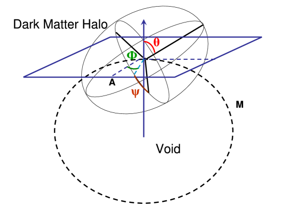
Figure 1: Schematic illustration of the orientation of the dark matter halo in the void surface. The position of three axes of the dark matter halo are characterised by the Euler angles ($\theta$, $\psi$, $\phi$). A, M are the local parallel and meridian, respectively.

If the shape of the halos were not aligned with any particular direction, $\cos\theta$, $\psi$, and $\phi$ will be distributed uniformly. However, the numerical simulations have shown that halos are not oriented randomly within the large scale structure. The probability distribution of $\theta$ has been explored by mean of several simulations. In the particular case of halos within a shell with a thickness of 4 h^-1Mpc around voids larger than 10 h^-1Mpc (defined by not containing halos with masses larger than 7.6 $\times$10¹¹h^-1M_☉), the simulations have shown that this probability distribution can be well described by the following expression:

$$P(\mu)d\mu=\frac{pd\mu}{[1+(p^{2}-1)\mu^{2}]^{3/2}};\mu\equiv cos\theta$$ (1)

with p a free parameter that is found to be 1.111$\pm$0.004 (see e.g. Cuesta et al. 2008). Cuesta et al. (2008) also have studied in the simulations the distribution of the angle $\psi$. They found that the distribution have a small, but highly significant, departure from uniformity. Given the small amplitude of this non-uniformity, we propose the following expression containing the simplest $\psi$ dependent term which is even with respect to $\psi=\pi$/2. This is a condition that must be satisfied due to the symmetry of the problem.

$$P(\psi)d\psi=\frac{2}{\pi}(1+\beta\cos(2\psi))d\psi$$ (2)

This expression is able to describe fairly well the data from the simulations with $\beta$=-0.093$\pm$0.005. This means that it is more likely to find the minor axis perpendicular to the intersection of the plane of the void with the plane defined by the middle and minor axes than parallel to this intersection. The opposite is obviously true for the middle axis.

Note that in the above expression $\psi$ is assumed to take values between 0 and $\pi$/2. As we mentioned above, $\psi$ actually goes between 0 and $\pi$, but due to the symmetry of P($\psi$) around $\psi$=$\pi$/2 it is not necessary to consider values of $\psi$ larger than $\pi$/2 (even though the position $\psi$ is not, in general, equivalent to $\pi$-$\psi$). However, we would like to stress that in the process of deriving the forthcoming mathematical identities $\psi$ is assumed to go from 0 to $\pi$ and it is only in the final expressions that the symmetry of P($\psi$) is exploited, so that in all the final expressions $\psi$ is assumed to be between 0 and $\pi$/2.

From the two expressions we have stated before, it follows that the full statistical information about the orientation of the halos with respect to the void is encoded in the joint probability distribution for $\cos(\theta)$ and $\psi$: P_or($\cos\theta$,$\psi$). We drop the dependence on $\phi$ since it is trivial. We propose the following expression to combine the above two probabilities, P($\cos\theta$) and P($\psi$):

$$P_{or}(\cos\theta,\psi)d\cos\theta d\psi=\left(\frac{p}{[1+(p^{2}-1)\cos^{2}\theta]^{3/2}}\right)$$

$$\left(\frac{2}{\pi}(1-\beta^{\prime}\sin^{2}\theta+2\beta^{\prime}\sin^{2}\theta\cos^{2}\psi)\right)d\cos\theta d\psi;\theta,\psi\in[0,\pi/2]$$ (3)

The first parenthesis corresponds to the probability distribution for $\cos\theta$ (Eq. 1) and the second parenthesis to the conditional probability distribution P($\psi$$\mid$$\theta$) for $\psi$ for a given value of $\theta$. To relate the parameter $\beta^{\prime}$ with $\beta$ we applied the fact that, for the halos under consideration (p=1.11), marginalising the above probability P_or with respect to $\cos\theta$, Eq. 2 must be obtained. On doing this we obtain: $\beta^{\prime}$=1.483$\beta$.

We may now note that the same physical cause (the shear of the velocity field) originates the departure of the distribution of $\cos\theta$ and $\psi$ from uniformity. Both effects are of the same order on the shear. Consequently, to leading order the quantity determining the departure from uniformity of $\cos\theta$ (i.e. $p-1$) must be proportional to the quantity determining the departure of $\psi$ from uniformity (i.e. $\beta^{\prime}$). We may use then Eq. 3 with:

$$\beta^{\prime}=-1.22(p-1)$$ (4)

From general considerations about the mechanisms generating the alignments one should expect this expression to be valid not only for the voids used to calibrate this expression but also for different voids, and also for halo alignments with respect to other large scale structures.

Using Eq. 3 we may obtain any statistic concerning the orientation of the halos with respect to the voids. For example, the alignment of the minor and middle axes with the radial direction (that has been already measured in simulations) can be expressed in terms of expression 3. The probability distribution, P_min($\cos\gamma$), for the cosine of the angle $\gamma$ between the minor axis and the radial direction of the void is related to P_or by the following expression:

$$P_{min}(\cos\gamma)=\int_{0}^{1}\int_{0}^{1}P^{{}^{\prime}}_{or}(\cos\theta,\cos\psi)\delta(\sin\theta\sin\psi-\cos\gamma)d\cos\theta d\cos\psi$$ (5)

where the Dirac’s $\delta$ distribution implement the constraint (based on spherical geometry) that only those values of $\theta$ and $\psi$ corresponding to an orientation of the halo in which the cosine of the angle between the minor axis and the radial direction take the value $\cos\gamma$ contribute to the integral. P${}^{{}^{\prime}}_{or}$ is simply the distribution implied by P_or for the variables $\theta$ and $\psi$:

$$P_{or}(x,y)\equiv\frac{P^{{}^{\prime}}_{or}(x,\arccos y)}{\sqrt{1-y^{2}}}$$ (6)

Carrying out the integral over $\psi$ we find:

$$P_{min}(\cos\gamma)=\cos\gamma\int_{\pi/2-\gamma}^{\pi/2}P^{{}^{\prime}}_{or}(\cos\theta,\frac{\sqrt{\sin^{2}\gamma-\cos^{2}\theta}}{\sin\theta})\frac{d\theta}{\sqrt{\sin^{2}\gamma-\cos^{2}\theta}}$$ (7)

In a similar fashion, simply changing $\sin\psi$ by $\cos\psi$ in the argument of the Dirac $\delta$ distribution, we find for the probability distribution, P_mid($\cos\eta$), for the cosine of the angle $\eta$ between the middle axis and the radial direction:

$$P_{mid}(\cos\eta)=\int_{\pi/2-\eta}^{\pi/2}P^{{}^{\prime}}_{or}(\cos\theta,\cos\eta/\sin\theta)d\theta$$ (8)

Using here expression 3 with $\beta^{{}^{\prime}}$=-0.134 and p=1.11, which is the value corresponding to the halos studied by Cuesta et al. (2008) we recover (see Fig. 2) the distributions $P_{mid}$ and $P_{min}$ determined directly in that work.

Figure 2: $Upper$ $panel$. The solid line is the probability distribution, P_min(cos$\gamma$), for the cosine of the angle $\gamma$ between the minor axis and the radial direction of the void as given by expression 5 with $\beta^{{}^{\prime}}$=-0.134 and p=1.11 (see text for details). The dashed line is the analytic fit to the results from the simulations by Cuesta et al. (2008) given by Eq. 1 using p=0.884. $Lower$ $panel$. The solid line is probability distribution, P_mid(cos$\gamma$), for the cosine of the angle $\gamma$ between the middle axis and the radial direction of the void as given by expression 8 of $\beta^{{}^{\prime}}$=-0.134 and p=1.11 (see text for details). The dashed line is the analytic fit to the results from the simulations by Cuesta et al. (2008) given by Eq. 1 using p=1.023.

3 Alignment of the angular momentum of the halo with respect to the halo axes

The alignment of the angular momentum of the halo with respect to their axes have been studied in detail in simulations (Bailin & Steinmetz 2005; Gottlöber & Turchaninov 2006; Patiri et al. 2006). We shall now consider a simple analytic model able to fit these alignments. To this end we take into account a set of halos with principal moments of inertia I₁, I₂ and I₃. Assuming that halos can interchange rotational kinetic energy and that they have reached statistical equilibrium, the probability distribution for the three components of the angular momentum J₁, J₂ and J₃ along the principal axes is proportional to the Boltzmann factor:

$$P(\vec{J})\propto\exp{\left\{-\left(\sum_{i=1}^{3}\frac{J_{i}^{2}}{2I_{i}}\right)/kT\right\}}$$ (9)

Let’s write the components of $\vec{J}$ in terms of its modulus J, the angle $\theta_{J}$ between $\vec{J}$ and the halo major axis, and the angle $\phi_{J}$ between the projection of $\vec{J}$ onto the plane perpendicular to the halo major axis and the halo minor axis. Integrating over J we find for the probability distribution P_J($\cos\theta_{J}$,$\phi_{J}$):

$$P_{\bf{J}}(\cos\theta_{J},\phi_{J})=\frac{3}{2}\frac{2}{\pi\sqrt{\bar{I}_{2}\bar{I}_{3}}}$$

$$\frac{1}{\left[\bar{I}_{2}^{-1}+\left(\bar{I}_{3}^{-1}-\bar{I}_{2}^{-1}\right)\cos^{2}\phi_{J}+\left(1-\bar{I}_{2}^{-1}-\left(\bar{I}_{3}^{-1}-\bar{I}_{2}^{-1}\right)\cos^{2}\phi_{J}\right)\cos^{2}\theta_{J}\right]}$$ (10)

with $\bar{I}_{2}$$\equiv\frac{I_{2}}{I_{1}}$ and $\bar{I}_{3}$$\equiv\frac{I_{3}}{I_{1}}$ and $\theta_{J}\in[0,\pi/2]$ and $\phi_{J}\in[0,\pi/2]$.

If the distribution of rotational kinetic energy amongst halos were in statistical equilibrium, setting in this expression the mean values of $\bar{I}_{2}$ and $\bar{I}_{3}$ ($\bar{I}_{2}$=1.38; $\bar{I}_{3}$=1.58, derived from the results of Jing & Suto 2000) one would obtain a good approximation to the actual distribution, since the dispersions of $\bar{I}_{2}$ and $\bar{I}_{3}$ are not too large. However, this is not what is observed in the simulations, because the actual distribution of the angular momentum is far from statistical equilibrium. Nonetheless, Eq. 10 can be used as a good model for the angular momentum distribution found in the simulations using the following values: $\bar{I}_{2}$=2.74 and $\bar{I}_{3}$=7.41. On doing this, we find: $<\cos\theta_{J1}>$=0.315; $<\cos\theta_{J2}>$=0.471 and $<\cos\theta_{J3}>$=0.671 where $\theta_{J1}$, $\theta_{J2}$ and $\theta_{J3}$ stands, respectively, for the angle between the angular momentum vector and the major, middle and minor halo axes. These numbers can be compared with the values found in the simulations for randomly chosen halos: 0.32, 0.48 and 0.69 (Cuesta et al. 2008). In those simulations it has been also found that above 75% of halos have $\theta_{J1}$ larger than 60 degrees. Eq. 10 predicts 73.5%.

3.1 Alignment of the angular momentum of the halo with respect to the halo axes for a given orientation of the halo with respect to the void

The above expression gives the probability distribution for the orientation of $\vec{J}$ with respect to the halo axes regardless of the orientation of the halo itself with respect to the large scale structure. However, from theoretical considerations we know that the distribution of $\theta_{J}$ and $\phi_{J}$ depends on the orientation of the halo. We shall show later (in the next subsection) that for halos in the shell of the voids considered by Cuesta et al. (2008), the probability distribution P_J($\theta_{J}$,$\phi_{J}$$\mid$$\theta$,$\psi$) for the angles $\theta_{J}$ and $\phi_{J}$ in those halos whose major axis form an angle $\theta$ with the radial direction of the void may be approximated by:

$$P_{\bf{J}}(\cos\theta_{J},\phi_{J}\mid\theta,\psi)=\frac{0.222}{\pi/2}$$

$$\frac{(F1\times F2\times F3)^{-1/2}}{[0.365F2+(0.135F3-0.365F2)\cos^{2}\phi_{J}+(F1-0.365F2-(0.135F3-0.365F2)\cos^{2}\phi_{J})\cos^{2}\theta_{J}]^{3/2}}$$ (11)

with F1$\equiv$1+$\alpha$($\cos^{2}\theta$-1/3), F2$\equiv$1+$\alpha$($\sin^{2}\theta$$\cos^{2}\psi$-1/3), F3$\equiv$1+$\alpha$($\sin^{2}\theta$$\sin^{2}\psi$-1/3) and $\alpha$=-0.68 ($\theta_{J}\in[0,\pi/2]$ and $\phi_{J}\in[0,\pi/2]$). This expression implies that for $\theta$=0 and any value of $\psi$ (which corresponds to have the major axis oriented in the void radial direction with the other two axes lying in the void plane): $<\cos\theta_{J1}>$=0.251; $<\cos\theta_{J2}>$=0.489 and $<\cos\theta_{J3}>$=0.693. For $\theta$=$\pi$/2 and $\psi$=$\pi$/2 (which corresponds to have the major and the middle axes in the plane of the void and the minor axis oriented in the void radial direction) we find $<\cos\theta_{J1}>$=0.354; $<\cos\theta_{J2}>$=0.526 and $<\cos\theta_{J3}>$=0.598.

From the above numbers we see that the mean values of $<\cos\theta_{J1}>$, being $\theta_{J1}$ the angle between $\vec{J}$ and the halo major axis, depends very substantially on the orientation of the halo with respect to the void. To understand the origin of this dependence we only need to consider the following: the axis corresponding to the smallest proper value of the shear of the velocity field associated with the void expansion is parallel to the radial direction of the void. This produces an extra component of $\vec{J}$ which is perpendicular to that direction. Consequently, when the halo major axis is parallel to the radial direction ($\theta$=0), the extra component of $\vec{J}$ is also perpendicular to the halo major axis. So, the average value $<\cos\theta_{J1}>$ for this particular configuration must be smaller than the average value over all halos: $<\cos\theta_{J1}>$=0.315. On the other hand, when $\theta$=$\pi$/2, the tendency of $\vec{J}$ to lay parallel to the surface of the void does not imply an obvious tendency for $<\cos\theta_{J1}>$. But, to compensate for the smaller value of $<\cos\theta_{J1}>$ when $\theta$=0, the mean value of $<\cos\theta_{J1}>$ when $\theta$=$\pi$/2 must be larger than for a randomly chosen halo.

The value of $\alpha$ given in expression 11 corresponds to the halos considered by Cuesta et al. (2008), but that expression can be made universally valid by simply expressing $\alpha$ as a function of p (the parameter measuring the strength of the alignment of the major axis with the radial direction):

$$\alpha=-8.64(p-1)$$ (12)

This relation should be valid in a general situation (with some reservations as presented in the discussion section) where both the orientation of the halos and their angular momentum are affected by a large scale shear of the velocity field.

It must be noted that, unlike Eq. 10, expression 11 has not been checked with numerical simulations. It has been derived from Eq. 10 assuming a simple model for the dependencies on $\theta$ and $\psi$ and fitting the value of $\alpha$. In this respect it may be considered a prediction for the dependence on $\theta$ and $\psi$ of the probability distribution for $\theta_{J}$ and $\phi_{J}$.

3.2 Alignment of the angular momentum of the halo with respect to the void radial direction

Having determined the probability distribution for the orientation of the halo with respect to the void, $P_{or}(\cos\theta,\psi)$, and the probability distribution for the orientation of the angular momentum with respect to the halo for a given orientation of the halo with respect to the void, $P_{\bf{J}}(\cos\theta_{J},\phi_{J}\mid\theta,\psi)$, we can now express the probability distribution $P_{\bf{J}}(\cos\mu)$ for the angle between $\vec{J}$ and the radial direction of the void in the following manner:

$$\bar{P}_{\bf{J}}(\cos\mu)=\frac{2}{64}\int_{-1}^{1}\int_{-1}^{1}\int_{0}^{2\pi}\int_{0}^{2\pi}P_{or}(\cos\theta,\psi)P_{\bf{J}}(\cos\theta_{J},\phi_{J}\mid\theta,\psi)$$

$$\delta(\cos\theta\cos\theta_{J}+\sin\theta\sin\theta_{J}\cos(\psi-\phi_{J})-\cos\mu)d\phi_{J}d\psi d\cos\theta d\cos\theta_{J}$$ (13)

The factor 1/64 comes from the fact that the distributions $P_{or}$ and $\bar{P}_{\bf{J}}$ are normalised with all angles between 0 and $\pi$/2. This is because, as long as we consider only the orientation of halos or the orientation of $\vec{J}$ within the halo, given the symmetries, this is the meaningful range for the angles. However, when we consider both orientations simultaneously to obtain the position of $\vec{J}$ with respect to the void we must consider all angles between 0 and $\pi$ to cover all possible configurations. The factor 2 comes from normalising $P_{J}(\cos\mu)$ to the range $\cos\mu\in$[0,1].

Integrating over $\phi_{J}$ and taking advantage of the symmetries of the integral, we find:

$$\bar{P}_{\bf{J}}(\cos\mu)=\frac{1}{8}\int_{0}^{\pi}\int_{-1}^{1}\int_{\cos(\theta+\mu)}^{\cos(\theta-\mu)}$$

$$\frac{P_{or}(\cos\theta,\psi)P_{\bf{J}}(\cos\theta_{J},\phi_{J}\mid\theta,\psi)d\cos\theta_{J}d\cos\theta d\psi}{\sqrt{(\sin\theta\sin\theta_{J})^{2}-(\cos\mu-\cos\theta\cos\theta_{J})^{2}}}$$ (14)

with $\phi_{J}\equiv\arccos((\cos\mu-\cos\theta\cos\theta_{J})/(\sin\theta\sin\theta_{J}))+\psi$.

Figure 3: The thick solid line is the probability distribution, $\bar{P}_{\bf{J}}$($\cos\mu$), for the cosine of the angle $\mu$ between the angular momentum vector of the halo $\vec{J}$ and the radial direction of the void as given by Eq. 14 with P_or given by Eq. 3 and P_J given by Eq. 11; The dot line represents the unconditional model which is estimated as above but using all F’s equal to one in Eq.11. The dashed line is the analytic fit to the results from the simulations by Cuesta et al. (2008) given by Eq. 1 using p=1.029.

If we assumed that the orientation of the angular momentum with respect to the halo is not affected by the orientation of the halo with respect to the void, the conditional distribution, $P_{\bf{J}}(\cos\theta_{J},\phi_{J}\mid\theta,\psi)$, would be equal to the unconditional one $P_{\bf{J}}(\cos\theta_{J},\phi_{J})$ given by Eq. 10 with $\bar{I}_{2}$=2.74 and $\bar{I}_{3}$=7.41. Then using Eq. 3 with $\beta^{{}^{\prime}}$=-0.134 for $P_{or}$, which corresponds to the halos around the large voids studied by Cuesta et al. (2008), and inserting both distributions into expression 13 we would not recover the distribution for $\cos\mu$ found in the simulations, which is well parametrised by:

$$P_{\bf{J}}(\cos\mu)=\frac{p}{(1+(p^{2}-1)\cos^{2}\mu)^{3/2}}$$ (15)

with p=1.029. Instead, we obtain an alignment with the opposite sign (see Fig. 3).

To reproduce the observed distribution we must allow for a dependence of $P_{\bf{J}}$ on $\theta$ and $\psi$. A simple model for this dependence has been given in the previous subsection (see Eq. 11). Inserting this into expression 14 together with expression 3 with $\beta^{{}^{\prime}}$=-0.134 for $P_{or}$ we may fit $\alpha$ so as to obtain the best fit (with $\alpha$=-0.68) to the numerical results which are well described by Eq. 15. This is how we have obtained the value of $\alpha$ given in 11. It must be noted that this expression represent a model in which, for any value of $\theta$, $\psi$ the alignment of $\vec{J}$ with the axes follows expression 10 (corresponding to randomly chosen halos), but where the parameters show a small dependence on $\theta$ and $\psi$ (the simplest with the right symmetry).

The fact that expression 14, with expression 3 and 11 for P_or, P_J, respectively, agrees with 15 to a high degree of accuracy for any value of $\cos\mu$ confirms the validity of this model for the conditional $P_{\bf{J}}$ (see Fig. 3).

If the two distributions entering expression 14 were independent of $\psi$ and $\phi_{J}$, i.e. if they take the following form:

$$P_{1}(\theta,\psi)=\frac{1}{\pi}P_{1}(\cos\theta)$$

$$P_{2}(\theta,\psi)=\frac{1}{\pi}P_{2}(\cos\theta_{J}\mid\theta)$$ (16)

both normalised with all angles between 0 and $\pi$, then expression 14, after integrating over $\psi$, reduces to:

$$P(\cos\mu)=\frac{1}{2\pi}\int_{-1}^{1}\int_{\cos(\theta+\mu)}^{\cos(\theta-\mu)}\frac{P_{1}(\cos\theta)P_{2}(\cos\theta_{J}\mid\theta)d\cos\theta_{J}d\cos\theta}{\sqrt{\sin^{2}\theta\sin^{2}\theta_{J}-(\cos\mu-\cos\theta\cos\theta_{J})^{2}}}$$ (17)

This expression gives the probability distribution for the angle $\mu$ between a fixed vector $\vec{H}$ and a vector $\vec{a}$ determined as follows: choose a vector $\vec{b}$ which forms and angle $\theta$ with $\vec{H}$ with a probability distribution given by P₁ and a randomly chosen (uniformly) azimuthal angle. Then, choose the vector $\vec{a}$ forming an angle $\theta_{J}$ with $\vec{b}$ with a probability distribution given by P₂ and a randomly (uniformly) distributed azimuthal angle.

In the case where P₂ does not depend on $\theta$ this expression is symmetric in P₁ and P₂. This is not evident at first sight, given the different integration limits for $\theta$ and $\theta_{J}$. $P(\cos\mu)$ can be seen as the two-dimensional convolution on the sphere of P₁ and P₂. We will use this expression in the next section to study the effect of the dilution of the signal of the alignments due to: a) the miss-aligning processes after the moment of turn-around and b) the observational errors in the estimation of $\theta$.

4 Degradation of the alignments

4.1 Degradation of the alignments due to the miss-aligning process after the moment of turn-around

In the standard (linear) tidal torque theory (TTT), the torque acting on a protohalo keeps its direction invariant through the time. It has been found in numerical simulations that the TTT predicts correctly the angular momentum of the protohalo up to the moment of the turn-around (Porciani et al. 2002). Hereafter, the tidal torque starts to rotate so by the time the halo virialises, its angular momentum will form an angle $\zeta$ with respect to the initial torque. The initial torque direction is close to the direction of the angular momentum at the moment of the turn-around. This evolutionary process has been studied in detail by Porciani et al. (2002). We have found that the distribution of the angle $\zeta$ that they found can be approximated by:

$$P(\zeta)\simeq 16.83[e^{-\sin\zeta/0.21}(1-\Theta(\zeta-\pi/2))+0.0085\Theta(\zeta-\pi/2)]\sin\zeta$$ (18)

where $\Theta$ is the Heaviside function.

Assume now that we have derived the theoretical predictions for the alignment of $\vec{J}$ with the large scale structure under the assumption of a non-rotating torque, whose probability distribution we represent by $P^{{}^{\prime}}_{\bf{J}}$ (that turns out to be given by Eq. 15 with a certain value of p). To obtain the probability distribution, $P_{\bf{J}}$, corresponding to the alignment of the actual $\vec{J}$ we must take into account the fact that the angular momentum of the halo is rotated by an angle $\zeta$ with respect to the theoretical prediction. Consequently,P_J may be expressed as the convolution on the sphere of $P^{{}^{\prime}}_{\bf{J}}$ and 2$P(\zeta)$, which is given by expression 17 with these two distributions in the place of P₁ and P₂. The factor 2, in 2$P(\zeta)$, is due to the fact that $P(\zeta)$, which is not symmetric with respect to $\pi$/2, is not normalised within the interval (0,$\pi$/2), unlike the distribution appearing in Eq. 17.

Figure 4: The thick solid line is the probability distribution, ${P}_{\bf{J}}$($\cos\mu$), for the cosine of the angle $\mu$ between the angular momentum vector of the halo $\vec{J}$ and the radial direction of the void accounting for the tidal torque rotation during and after the formation of the halo. To estimate the effect of the rotation of the tidal torque, we have assumed that, under the assumption of a non-rotating torque, ${P}_{\bf{J}}$($\cos\mu$) is given by Eq. 15 with p=1.06 and we have convolved this expression with Eq. 18 using Eq. 17. The dashed line is the analytic fit to the results from the simulations by Cuesta et al. (2008) given by Eq. 1 using p=1.03. We find that the strength of the alignment, which is measured by p-1, reduces to a half with respect to the theoretical prediction under the assumption of a non-rotating torque.

If we use for $P^{{}^{\prime}}_{\bf{J}}$ a value of p=1.06, the resulting $P_{\bf{J}}$ (see Fig. 4) is also well approximated by expression 15 with a value of p of 1.03. So, we see that the strength of the alignment, which is measured by p-1, reduces to a half with respect to the theoretical predictions with a non rotating torque. This ratio between the value of p-1 for $P^{{}^{\prime}}_{\bf{J}}$ and $P_{\bf{J}}$ is constant to a very good approximation for all interesting p values (p-1$\ll$1).

Note that in obtaining $P_{\bf{J}}$ from $P^{{}^{\prime}}_{\bf{J}}$ and $P(\zeta)$ we have assumed that the rotation of $\vec{J}$ with respect to its primordial direction is independent of the orientation with respect to the large scale structure. This is a good approximation, because the large scale makes up only a small contribution to the total tidal field, and this contribution rotates less than that due to smaller scales.

4.2 Degradation of the alignment due to observational errors at estimating $\theta$

When measuring alignments between the large scale structure and the rotational axis of spiral galaxies, the error in the estimation of the alignment angle due to uncertainties in the position of the galaxies and in the orientation of its axis leads also to a degradation of the intrinsic alignment.

To quantify the relevance of this potential source of degradation of the alignment, we assume that the probability distribution, $P_{er}(\zeta)$, for the angle $\zeta$ between the observed and the actual direction of $\vec{J}$ takes the form:

$$P_{er}(\zeta)=\frac{e^{\frac{-\zeta^{2}}{2\sigma^{2}}}\sin\zeta}{\int_{0}^{\pi}e^{\frac{-\mu^{2}}{2\sigma^{2}}}\sin\mu d\mu}$$ (19)

Assuming again that the distribution of the angle $\zeta$ is independent of the large scale structure, we may insert in expression 17, 2$P_{er}(\zeta)$ and the probability distribution for the intrinsic alignment of the axes, $P_{in}(\cos\mu)$, to obtain the distribution for the observed $\mu$, $P_{ob}(\cos\mu)$. Using for $P_{in}$ expression 15 with p=1.06, we have obtained $P_{ob}$ for four values of $\sigma$ (see Fig. 5). Expected typical uncertainties in the observations, $\sigma\sim$20 degrees, do not produce a strong decrease in the signal.

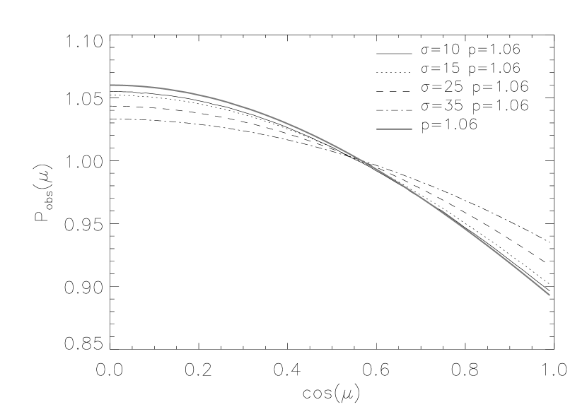
Figure 5: The different lines shows the probability distribution, $P_{obs}(\mu)$, for the angle $\mu$ between the observed angular momentum vector of the spiral galaxies $\vec{J}$ and the radial direction of the void assuming four different levels of uncertainty on the angular position of $\vec{J}$ ($\sigma$=10; $\sigma$=15; $\sigma$=25 and $\sigma$=35 degrees). The distribution for the intrinsic alignment of the angular momentum is given by Eq. 15 with p=1.06, whereas the observed distribution is characterised by the convolution, as provided by Eq. 17, between the intrinsic signal and the error function given by Eq. 19.

5 Discussion and Conclusions

We have presented a set of general tools for the description of the alignments of halos and galaxies with respect to the large scale structure where they are embedded. Using these tools we have done the following:

• We have provided an accurate model for the conditional probability distribution function for the orientation of the angular momentum with respect to the halo axis for halos with a given orientation with respect to the large scale structure. We have fitted the single parameter of our model so as to obtain, using the appropriate mathematical identity, the alignment between the angular momentum of the halos in the shells of cosmic voids that has been found in simulations. The conditional PDF obtained in this manner shows a strong dependence on the orientation of the halo with respect to the void. This dependence is produced by the tidal field on the shell of the voids which causes the minor axis to be more aligned with the radial direction than in the isotropic case, while the opposite is true for angular momentum. If that dependence did not exist, that is, if the PDF for the orientation of the angular momentum with respect to halo axis for halos in the shells of voids were the same as for randomly chosen halos (i.e. following an unconditional PDF) then the angular momentum would show the same kind of alignment with the radial direction than the minor axis and opposite to that found in simulations. In the past, and under the assumption that the angular momentum PDF is independent of the environment, there has been some confusion when interpreting the alignments of halo axis and angular momentum with the void radial direction.

• We have shown that the strength of the predicted alignment of the angular momentum with the void radial direction, as given by the TTT, it is twice as large as the one actually measured in simulations (as parametrised in this work by p-1). To model this degradation of the signal we have convolved the angular momentum PDF characterised by a certain parameter p (Eq. 1) with an analytical fit (based on previous results) that describes the PDF for the angle between the initial torque and the present angular momentum (Porciani et al. 2002). As long as p-1$\ll$1 the resulting distribution is also well described by the expression given in Eq. 1 with a value of p^′ such that 1-p^′=(1-p)/2. Understanding this degradation is a necessary step towards a fully theoretical explanation of the alignment of the angular momentum with the void radial direction found in simulations. In a future work (Betancort-Rijo & Trujillo 2010) we shall show that the TTT predicts, for the voids under consideration, a value of the strength of p$\simeq$1.06 for the initial alignment, so a value of p$\simeq$1.03 should correspond to the alignment of the present angular momentum, as found in simulations.

• We have also convolved the initial angular momentum PDF with a Gaussian PDF to model the observational errors on measuring the angle between the angular momentum and the void radial direction. For real galaxies this error arises both from the uncertainty on estimating the direction of the galaxy rotation axis as well as from the error on determining the void radial direction due to the redshift distortion. We have shown that up to a r.m.s. of roughly 15% the intrinsic alignment is basically unaffected.

In the present work we have dealt explicitly with large cosmic voids, but all expressions may be used whenever the orientation of the halos or galaxies with respect to the large scale structure (or more precisely, the orientation with respect to the proper axes of the deformation tensor or the tidal tensor on large scale) is considered. In order to use the expressions proposed in this paper in more general cases, two considerations are in order. First, the PDF for the orientation of halos (Eq. 3) may show in general a dependence on $\phi$. Therefore, in any expression involving integrals of P_or, the dependence on $\phi$ must be considered and that expression must also be integrated over $\phi$ and divided by 2$\pi$. Second, the ratios $\beta$^′/(p-1) (see expression 4) and $\alpha$/(p-1) (see expression 12) have been determined using halos within certain shells of cosmic voids. However, from general considerations about the mechanisms generating the alignments it follows that these ratios should be essentially independent of the voids used (as long as p-1$\ll$1). In other cases (i.e. walls or filaments) the same considerations lead to the constancy of the first ratio. The effect described by the second ratio (i.e. the dependence on environment of the orientation of the angular momentum with respect to the halo axes) does not depend just on the present deformation tensor, but also on its deformation history (we will show that on Betancort-Rijo & Trujillo 2010). Therefore, its value could depend on the kind of structure considered. This dependence, though, should be expected to be small, but as much as it can be measured it might provide an interesting test for the standard (and non-standards) model of the large-scale structure formation.

References

- (1) Aragón-Calvo, M. A., van de Weygaert, R., Jones, B. J. T., van der Hulst, J. M., 2007, ApJ, 655, L5
- (2) Bailin, J., & Steinmetz, M., 2005, ApJ, 627, 647
- (3) Brunino, R., Trujillo, I., Pearce, F. R. & Thomas, P. A., 2007, MNRAS, 375, 184
- (4) Cuesta, A. J., Betancort-Rijo, J. E., Gottlöber, S., Patiri, S. G., Yepes, G. & Prada, F., 2008, MNRAS, 385, 867
- (5) Doroshkevich, A. G., 1970, Astrophysics, 6, 320
- (6) Gottlöber, S. & Turchaninov, V., 2006, in Mass Profiles and Shapes of Cosmological Structures, ed. G. A. Mamon et al. (EAS Publ. Ser. 20; Les Ulis: EDP Sciences), 25
- (7) Jing, Y. P. & Suto, Y., 2002, ApJ, 574, 538
- (8) Lee. J., 2004, ApJ, 614, L1
- (9) Lee, J., Erdogdu, P., 2007, ApJ, 671, 1248
- (10) Navarro, J. F., Abadi, M. G., Steinmetz, M., 2004, ApJ, 613, L41
- (11) Patiri, S. G., Cuesta, A. J., Prada, F., Betancort-Rijo, J., & Klypin, A., 2006, ApJ, 652, L75
- (12) Peebles, P. J. E., 1969, ApJ, 155, 393
- (13) Porciani, C., Dekel, A., Hoffman, Y., 2002, MNRAS, 332, 325
- (14) Schäfer, B. M., 2009, IJMPD, 18, 173
- (15) Sciama, D. W., 1955, MNRAS, 115, 2
- (16) Slosar, A., White, M., 2009, JCAP, 06, 009
- (17) Trujillo, I., Carretero, C., Patiri, S. G., 2006, ApJ, 640, L111
- (18) White, S. D. M., 1984, ApJ, 286, 38