Turbulence, Energy Transfers and Reconnection in Compressible Coronal Heating Field-line Tangling Models

Abstract

MHD turbulence has long been proposed as a mechanism for the heating of coronal loops in the framework of the Parker scenario for coronal heating. So far most of the studies have focused on its dynamical properties without considering its thermodynamical and radiative features, because of the very demanding computational requirements. In this paper we extend this previous research to the compressible regime, including an energy equation, by using HYPERION, a new parallelized, viscoresistive, three-dimensional compressible MHD code. HYPERION employs a Fourier collocation – finite difference spatial discretization, and uses a third-order Runge-Kutta temporal discretization. We show that the implementation of a thermal conduction parallel to the DC magnetic field induces a radiative emission concentrated at the boundaries, with properties similar to the chromosphere–transition region–corona system.

1 INTRODUCTION

Magnetohydrodynamic turbulence in the framework of the Parker scenario for coronal heating Parker (1972, 1988) has been a very challenging problem to investigate numerically Dmitruk & Gómez (1999); Einaudi and Velli (1999); Einaudi et al. (1996); Hendrix and Van Hoven (1996); Rappazzo et al. (2007, 2008). As computers have advanced, it has become more feasible to do the large storage compressible problem.

Why is it important to include compressibility and its related effects? There are three basic categories of interest with respect to active region loops and the coronal heating problem, viz.: structural, dynamical and thermodynamical. The most significant structural effect is stratification due to gravity. We can also modify this term to model the curvature of a typical loop. Among new dynamical effects that are possible are compression and rarefaction of the plasma, as well as the formation of shocks.

Thermodynamical effects include thermal conduction and radiation. In addition, the diffusivities can be temperature dependent. It’s important to have these features in the model to begin to reproduce the energy cycle: kinetic energy in the photosphere is transformed into magnetic energy in the corona by means of photospheric footpoint convection. It is then transported to small scale by MHD turbulence, where through magnetic reconnection it is converted into thermal, kinetic and perturbed magnetic energies. Heat is then conducted from the high temperature corona back toward the low temperature photosphere, where it is lost via optically thin radiation.

Incompressible and cold plasma models only contain the first few parts of this energy cycle, without taking into account the thermodynamics. Any magnetic energy lost through Ohmic diffusion and any kinetic energy lost through viscous diffusion is simply lost from the system and the physics involved with thermal conduction and radiation is irrelevant.

Our new compressible code HYPERION has allowed us to make a start at examining the fully compressible, three-dimensional Parker coronal heating model. HYPERION is a parallelized Fourier collocation–finite difference code with third-order Runge-Kutta time discretization that solves the compressible MHD equations with DC field–aligned thermal conduction and radiation included.

2 SETTING UP THE PROBLEM

2.1 Governing equations

We model the solar corona as a compressible, dissipative magnetofluid. The equations which govern such a system, written here in a dimensionless form, are:

$$\frac{\partial\rho}{\partial t}=-\nabla\cdot(\rho{\bf v})$$ (1)

$$\frac{\partial\rho{\bf v}}{\partial t}=-\nabla\cdot({\rho\bf vv})-{\beta}\nabla p+{\bf J}\times{\bf B}+\frac{1}{S_{v}}\nabla\cdot\mathbf{\zeta}$$ (2)

$$\qquad\qquad\qquad\qquad\qquad\qquad\qquad+\rho g(z){\bf\hat{e}}_{z}$$ (3)

$$\frac{\partial T}{\partial t}=-{\bf v}\cdot\nabla T-(\gamma-1)(\nabla\cdot{\bf v})T+\frac{1}{Pr\,S_{v}}\frac{1}{\rho}\frac{\partial^{2}T}{\partial z^{2}}+f$$ (4)

$$\frac{\partial{\bf B}}{\partial t}=\nabla\times{\bf v}\times{\bf B}+\frac{1}{S}\nabla\times\nabla\times{\bf B}$$ (5)

$$\nabla\cdot{\bf B}=0.$$ (6)

where $f={(\gamma-1)\over\beta\rho}[{1\over S_{v}}\zeta_{ij}{\bf e}_{ij}+{1\over S}(\nabla\times{\bf B})^{2}-{1\over S_{r}}\rho^{2}\Lambda(T)].$ The system is closed by the equation of state,

$$p=\rho T.$$ (7)

In the preceding equations the variables are defined in the following way:   $\rho({\bf x},t)$ is the mass density, ${\bf v}({\bf x},t)=(u,v,w)$ is the flow velocity, $p({\bf x},t)$ is the thermal pressure, ${\bf A}({\bf x},t)=(A_{x},A_{y},A_{z})$ is the magnetic vector potential, ${\bf B}({\bf x},t)=(B_{x},B_{y},B_{z})=\nabla\times{\bf A}$ is the magnetic induction field expressed in terms of the associated Alfvén velocity (${\bf B}\rightarrow{\bf B}/\sqrt{4\pi\rho_{0}}$), ${\bf J}=\nabla\times{\bf B}$ is the electric current density, $T({\bf x},t)$ is the plasma temperature, $\zeta_{ij}=\mu(\partial_{j}v_{i}+\partial_{i}v_{j})-\lambda\nabla\cdot{\bf v}\delta_{ij}$ is the viscous stress tensor, $e_{ij}=(\partial_{j}v_{i}+\partial_{i}v_{j})$ is the strain tensor, and $\gamma$ is the adiabatic ratio. The thermal conductivity ($\kappa$), magnetic resistivity $(\eta)$, and shear viscosity $(\mu)$ are assumed to be constant and uniform, and Stokes relationship is assumed so the bulk viscosity $\lambda=(2/3)\mu$. The function $g(z)$ defines the gravitational field strength: at $t=0$ we define $\rho$ as $\rho_{0}\exp[-{1\over 2}g\cos({\pi z\over L_{z}})]$. Assuming a uniform temperature we can determine the gravity as $g=\beta{1\over\rho}{d\rho\over dz}.$ The function $\Lambda(T)$ describes the temperature dependence of the radiation ($\Lambda(T)=0$ for $T<T_{0}$):

$$\Lambda(T)=\frac{T-T_{0}}{T_{0}}e^{(\epsilon T-T_{0})/(\tau T_{0})},\qquad T\geq T_{0}$$ (8)

where $T_{0}$ is the wall (photospheric) temperature, $\epsilon=2$ and $\tau=2$ (Dahlburg et al. (1987); Dahlburg and Mariska. (1988)). The important dimensionless numbers are: $S_{v}=\rho_{0}V_{A}L_{0}/\mu\equiv$ viscous Lundquist number, $S=V_{A}L_{0}/\eta\equiv$ Lundquist number, $S_{r}=V_{A}L_{0}/\chi\equiv$ radiative Lundquist number (the new parameter $\chi$ determines the strength of the radiation), $\beta=p_{0}/B_{0}^{2}\equiv$ pressure ratio at the wall, $Pr=C_{p}\mu/\kappa\equiv$ Prandtl number, and $A=V_{A}/V_{0}\equiv$ Alfvén number. In these definitions, $\rho_{0}$ is a characteristic density, $V_{A}$ is the vertical Alfvén speed (used as the characteristic velocity to render velocities dimensionless), $L_{0}$ is the vertical box length ($=L_{z}$), $C_{p}$ is the specific heat at constant pressure, $C_{s}$ is the free-stream sound speed, and $V_{0}$ is the characteristic flow speed. Time ($t$) is measured in units of Alfvén transit times ($=L_{0}/V_{A}$).

Boundary Conditions and Forcing

We solve the governing equations in a box of dimensions ($L_{x},L_{y},L_{z}$). The system has periodic boundary conditions in $x$ and $y$, and line-tied boundary conditions in $z$. To model a section of a coronal loop the system is threaded by a DC magnetic field in the $z$-direction ($B_{0}$).

We then employ a simple, three-dimensional extension of the time-dependent forcing function used in the previous studies Hendrix et al. (1996); Einaudi and Velli (1999), i.e., at the top and bottom walls we evolve a stream function:

$$\psi_{nm}(x,y,t)=f_{1}\sin^{2}\left(\frac{\pi t}{2t^{*}}\right)+f_{2}\sin^{2}\left(\frac{\pi t}{2t^{*}}+\frac{\pi}{2}\right)$$ (9)

where $f_{i}(x,y)=V_{0}\sum_{n}\sum_{m}a_{nm}^{i}sin(k_{n}x+k_{m}y+\zeta_{nm}^{i}).$ Values for $k$ are given by $3\leq(k_{n}^{2}+k_{m}^{2})^{1\over 2}\leq 4$. At the top and bottom walls the magnetic vector potential is convected by the resulting flows.

That is, the line-tied boundary conditions are:

$$\rho(\pm L_{z}/2)=\rho_{0},$$

$$\rho u(\pm L_{z}/2)=-\rho_{0}\partial\psi/\partial y,$$

$$\rho v(\pm L_{z}/2)=\rho_{0}\partial\psi/\partial x,$$

$$\rho w(\pm L_{z}/2)=0,$$

$$\partial A_{x}/\partial t|_{\pm L_{z}/2}=v~{}B_{0},$$

$$\partial A_{y}/\partial t|_{\pm L_{z}/2}=-u~{}B_{0},$$

$$B_{z}(\pm L_{z}/2)=B_{0},$$

$$T(\pm L_{z}/2)=T_{0}.$$

The enforcement of the boundary conditions is discussed in greater detail in Dahlburg et al. (2007).

Numerics

Equations 5 and 6 can be replaced by the magnetic vector potential equation:

$$\frac{\partial{\bf A}}{\partial t}={\bf v}\times\nabla\times{\bf A}+\frac{1}{S}~{}\nabla\times\nabla\times{\bf A}$$ (10)

where ${\bf A}=\nabla\times{\bf B}.$ Thus we solve numerically the equations 1-3 and 7 together with equation 6. Space is discretized in $x$ and $y$ with a Fourier collocation scheme Dahlburg and Picone (1989) with isotropic truncation dealiasing. Spatial derivatives are calculated in the appropriate transform space, and nonlinear product terms are advanced in configuration space. A second-order central difference technique Dahlburg, Montgomery and Zang (1986) is used for the discretization in $z$. A staggered mesh also is employed in the $z$-directionSchnack et al. (1987). In general, the fields that are defined at the $z$ boundaries are advanced in time on the standard mesh. Other quantities of interest are defined and advanced in time on the staggered mesh. That is, on the standard mesh we look at $\rho,\rho u,~{}\rho v,~{}\rho w,~{}A_{x},~{}A_{y},~{}B_{z}$ and $T$. Some derived fields such as $\omega_{x},~{}\omega_{y},~{}\omega_{z},~{}j_{x},$ and $j_{y}$ are also defined on the standard mesh. On the staggered mesh we look at $A_{x},~{}B_{x},~{}B_{y},$ and $j_{z}$. Note that for plotting purposes we interpolate these latter fields onto the standard mesh (at the boundaries an extrapolation is performed).

A time-step splitting scheme is employed. All terms, with the exception of the vertical pressure gradient and the gravitation term, are discretized in time with a third-order Runge-Kutta scheme. The pressure step for the $z$-momentum is solved with a second-order Lax-Wendroff one-step central difference scheme. The vertical gravitation term is advanced using the forward Euler method.

The code has been parallelized using MPI. A domain decomposition is employed in which the computational box is sliced up into $x$–$y$ planes along the $z$ direction.

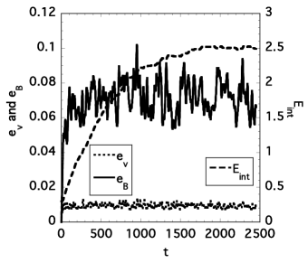
Figure 1: Energies vs. time. Time is measured in units of axial Alfvén crossing times $L_{z}/V_{A}$.

3 New results

In this section we report on the results of a preliminary numerical simulation of the model. This simulation is run with $L_{x}=2\pi,L_{y}=2\pi$ and $L_{z}=8\pi$. Other important parameters are $g=6.0,\gamma=5/3,S=S_{v}=80000,\beta=0.001,B_{0}=1.0,V_{0}=0.01(\sqrt{2}/2),A=V_{A}/V_{0}=100\sqrt{2},\rho_{0}=1.0,T_{0}=1.0,t^{*}=20.0,Pr=0.001$, and $S_{r}=0.0004$.

3.1 Temporal diagnostics

To insure that we are obtaining good statistics, the system has to settle down into a steady state. Evidence for this is shown in Figure 1, which shows some of the important energies as functions of time (time is expressed in units of Alfvén transit times $L_{0}/V_{A}$). As seen in our previous RMHD simulations, the fluctuating magnetic and kinetic energies ($e_{v}={1\over 2}\int_{-L_{z}/2}^{L_{z}/2}\int_{0}^{L_{y}}\int_{0}^{L_{x}}|{\bf v}|^{2}~{}dx~{}dy~{}dz$ and $e_{b}={1\over 2}\int_{-L_{z}/2}^{L_{z}/2}\int_{0}^{L_{y}}\int_{0}^{L_{x}}|{\bf b}|^{2}~{}dx~{}dy~{}dz$) settle down pretty quickly, with $e_{b}>e_{v}$ (these quantities are also time intermittent). Note, however, that the total internal energy $E_{int}={\beta\over\gamma-1}\int_{-L_{z}/2}^{L_{z}/2}\int_{0}^{L_{y}}\int_{0}^{L_{x}}\rho~{}T~{}dx~{}dy~{}dz$ takes much longer to level off in time. This reflects the fact that the system must heat up to attain the driven-dissipative steady state.

The quantities shown in Figure 2 provide temporal information about the dissipation. Note that the radiation loss is a new quantity respect to previous simulations. Shown are the enstrophy $\Omega={1\over S_{v}}\int_{-L_{z}/2}^{L_{z}/2}\int_{0}^{L_{y}}\int_{0}^{L_{x}}|{\bf\omega}|^{2}~{}dx~{}dy~{}dz$, mean square electric current $J=\frac{1}{S}\int_{-L_{z}/2}^{L_{z}/2}\int_{0}^{L_{y}}\int_{0}^{L_{x}}|{\bf j}|^{2}~{}dx~{}dy~{}dz$, and the total radiation losses $D={1\over S_{r}}\int_{-L_{z}/2}^{L_{z}/2}\int_{0}^{L_{y}}\int_{0}^{L_{x}}\rho^{2}~{}\Lambda(T)~{}dx~{}dy~{}dz$ as functions of time. The first two quantities behaves similarly to previous RMHD simulations, while the radiative losses settles on a similar timescale than the internal energy (Figure 1).

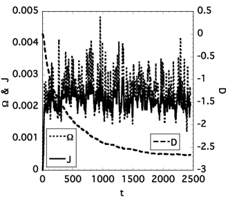
Figure 2: Dissipation vs. time. Time is measured in units of axial Alfvén crossing times $L_{z}/V_{A}$.

3.2 Spatial diagnostics

The following quantities are averaged over the perpendicular directions ($x$ and $y$) and also over $1000\leq t\leq 2000$. We look at these to determine the times averaged state of the system under unsteady heating.

We first look at some of the quantities related to the dissipation of the system. Figure 3 shows some of the time averaged quantities as a function of $z$, the direction of the large magnetic field $B_{0}$. Shown are the time averaged dissipation intensity for the parallel vorticity $Q_{z}(z)=<[\int_{0}^{L_{y}}\int_{0}^{L_{x}}{\omega_{z}^{2}}(x,y,z)\,dxdy]^{1\over 2}>$ and also for the parallel electric current $G_{z}(z)=<[\int_{0}^{L_{y}}\int_{0}^{L_{x}}{j_{z}}^{2}(x,y,z)\,dxdy]^{1\over 2}~{}>$ as well as the time averaged mean radiation rate $D_{m}(z)={1\over S_{r}}<\int_{0}^{L_{y}}\int_{0}^{L_{x}}\rho^{2}\Lambda(T)(x,y,z)\,dxdy>$. As in previous simulations, current density and vorticity are aligned to the dc magnetic field, so that their $z$-components are strongly dominant. Note that “$<~{}~{}>$” denotes the time averaging. The symmetry in $z$ of these quantities indicates that we have averaged over a sufficient period of time.

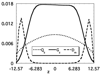
Figure 3: Time averaged dissipation rates (viscous $Q_{z}$, ohmic $G_{z}$ and radiative $D_{m}$) as a function of the axial coordinate z.

In Figure 4 we take a look at the time averaged thermodynamic state for the unsteady heating case: shown are the time averaged mean mass density $\rho_{m}(z)=<\int_{0}^{L_{y}}\int_{0}^{L_{x}}\rho(x,y,z)dxdy>$ and the time averaged mean temperature $T_{m}(z)=<\int_{0}^{L_{y}}\int_{0}^{L_{x}}T(x,y,z)dxdy>$ as functions of $z$.

The density profile is a result of the gravitational density stratification. Figures 3 and 4 show feature typical of the chromosphere-transition region-corona system, where density increases at lower heights, while temperature increases in the high corona. Notice that most of the ohmic and viscous dissipation ($Q_{z}$ and $G_{z}$) takes place in the high corona, while radiation ($D_{m}$) origins mostly near the boundaries, where it is peaked (see Figure 3). This mostly results from the higher density values near the boundaries, as $\Lambda(T)$ is multiplied by $\rho^{2}$ in the radiative term $D_{m}$.

4 DISCUSSION

In this paper we have presented some preliminary results of our simulations of compressible DC coronal heating using our new HYPERION code. The inclusion of a thermal conductivity parallel to the DC magnetic field, coupled with a gravitational density stratification, gives rise to temperature and radiation features typical of a realistic coronal loop.

This is an encouraging starting point to investigate the thermodynamical properties of a coronal loop threaded by a strong magnetic field whose footpoints are shuffled by photospheric motions.

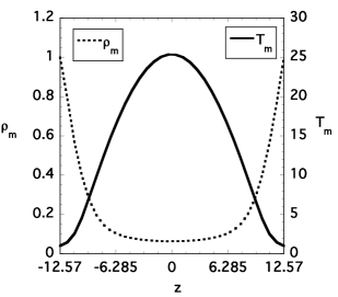
Figure 4: Time averaged mass density ($\rho_{m}$) and temperature ($T_{m}$) as a function of z.

References

- Dahlburg et al. (1987) Dahlburg, R. B., DeVore, C.R., Picone, J. M., Mariska, J. T., and Karpen, J. T. 1987, Astrophys. J., 315, 385
- Dahlburg and Mariska. (1988) Dahlburg, R. B., and Mariska, J. T. 1988, Solar Phys., 117, 51
- Dahlburg et al. (2007) Dahlburg, R. B., Liu, J. -H., Klimchuk, J. A., and Nigro, G. 2009, Astrophys. J.,in press
- Dahlburg, Montgomery and Zang (1986) Dahlburg, R. B., Montgomery, D. and Zang, T. A. 1986, J. Fluid Mech., 169, 71
- Dahlburg and Picone (1989) Dahlburg, R. B., and Picone, J. M. 1989, Phys. Fluids B, 1, 2153
- Dmitruk & Gómez (1999) Dmitruk, P., & Gómez, D. O. 1999, ApJ, 527, L63 Geophys. Res., 104, 521
- Einaudi and Velli (1999) Einaudi, G., and Velli, M., 1999, Phys. Plasmas, 6, 4146
- Einaudi et al. (1996) Einaudi, G., Velli, M., Politano, H., & Pouquet, A. 1996, ApJ, 457, L113
- Hendrix and Van Hoven (1996) Hendrix, D. L., and Van Hoven, G. 1996, Astrophys. J., 467, 887
- Hendrix et al. (1996) Hendrix, D. L., Van Hoven, G., Mikić, Z., and Schnack, D. D., 1996, Astrophys. J., 470, 1192
- Parker (1972) Parker, E. N. 1972, Astrophys. J., 174, 499
- Parker (1988) Parker, E. N. 1988, Astrophys. J., 330, 474
- Schnack et al. (1987) Schnack, D. D., Barnes, D. C., Mikic, Z. Harned, D. S., and Caramana, E. J. 1987, J. Comput. Phys., 70, 330
- Rappazzo et al. (2007) Rappazzo, A. F., Velli, M., Einaudi, G., and Dahlburg, R. B., 2007, Ap. J. Lett., 657, L47
- Rappazzo et al. (2008) Rappazzo, A. F., Velli, M., Einaudi, G., and Dahlburg, R. B., 2008, ApJ., 677, 1348