New physics reach of CP violating observables in the decay $\bar{B}_{d}\rightarrow\bar{K}^{*}\ell^{+}\ell^{-}$

Abstract:

We discuss theoretical and experimental preparations for an indirect new physics search using the rare decay $\bar{B}_{d}\rightarrow\bar{K}^{*0}(\rightarrow K\pi)\mu^{+}\mu^{-}$ focusing on CP violating observables. The separation of new physics effects and hadronic uncertainties is the key issue when using flavour observables in a new-physics search. Our analysis is based on QCD factorization and soft-collinear effective theory and critically examines the new physics reach of those observables via a detailed error analysis due to scale dependences, form factors, and other input parameters; we also explore the experimental sensitivities at LHCb using a full-angular fit method; finally, we make the impact of the unknown $\mathchar 28931\relax/m_{b}$ corrections manifest in our theoretical predictions.

1 Introduction

At the beginning of the LHC era and close to the end of the $B$ factories at SLAC [3] and at KEK [4] and of the Tevatron $B$ physics experiments [5, 6], all experimental data on flavour mixing and CP violating phenomena are consistent with the simple CKM theory of the standard model (SM) [7], which means that all flavour-violating processes between quarks are governed by a $3\times 3$ unitarity matrix, usually referred to as Cabibbo-Kobayashi-Maskawa (CKM) matrix [8]. The CKM matrix is fully described by four real parameters, three rotation angles and one phase. It is this phase that represents the only source of CP violation in the SM and that now allows for an unified description of all the CP violating phenomena. This is an impressive success of the SM and the CKM theory and can be illustrated by the overconstrained triangles in the complex plane which reflect the unitarity of the CKM matrix. The successful theory was honored by last year’s nobel prize in physics [9]. Thus, the CKM mechanism is the dominating effect for CP violation and flavour mixing in the quark sector; however, there is still room for sizable new effects and new flavour structures because the flavour sector has only been tested at the $10\%$ level especially in the $b\rightarrow s$ sector. In particular, CP violating observables are a good testing ground for new physics scenarios. While the SM is very predictive by describing all CP violating phenomena via one parameter, many new physics models offer many new CP phases.

In Ref. [10, 11], we worked out the theoretical and experimental preparations for an indirect new physics (NP) search using the rare decay $\bar{B}_{d}\rightarrow\bar{K}^{*}\ell^{+}\ell^{-}$ based on the QCDf/SCET approach: QCD corrections are included at the next-to-leading order level and also the impact of the unknown $\mathchar 28931\relax/m_{b}$ corrections is made explicit. The full angular analysis of the decay $\bar{B}_{d}\rightarrow\bar{K}^{*}(\rightarrow K^{-}\pi^{+})\ell^{+}\ell^{-}$ at the LHCb experiment offers great opportunities for the new physics search. New observables can be designed to be sensitive to a specific kind of NP operator within the model-independent analysis using the effective field theory approach. The new observables $A_{T}^{(2)}$, $A_{T}^{(3)}$, and $A_{T}^{(4)}$ are shown to be highly sensitive to right-handed currents. Moreover, it was shown that the previously discussed angular distribution $A_{T}^{(1)}$ cannot be measured at either LHCb or at a Super-$B$ factory.

In the present letter we extend this preparation work to CP violating observables in the rare decay. We already anticipate here that, in contrast to claims in the literature, the new physics reach of such CP violating observables is rather limited. More details of our analysis with further results will be published in a forthcoming paper [12].

2 CP asymmetries

The decay  $\overline{\kern-2.40005ptB}_{d}\rightarrow\kern 1.99997pt\overline{\kern-1.99997ptK}{}^{*0}\ell^{+}\ell^{-}$ with $\kern 1.99997pt\overline{\kern-1.99997ptK}{}^{*0}\rightarrow K^{-}\pi^{+}$ on the mass shell is completely described by four independent kinematic variables, the lepton-pair invariant mass squared, $q^{2}$, and the three angles $\theta_{l}$, $\theta_{K}$, $\phi$. Summing over the spins of the final particles, the differential decay distribution of  $\overline{\kern-2.40005ptB}_{d}\rightarrow\kern 1.99997pt\overline{\kern-1.99997ptK}{}^{*0}\ell^{+}\ell^{-}$ can be written as

$$\frac{d^{4}\Gamma}{dq^{2}\,d\cos\theta_{l}\,d\cos\theta_{K^{*}}\,d\phi}=\frac{9}{32\pi}J(q^{2},\theta_{l},\theta_{K^{*}},\phi)\,,$$ (1)

The dependence on the three angles can be made more explicit:

$$J(q^{2},\theta_{l},\theta_{K},\phi)= J_{1}^{s}\sin^{2}\theta_{K}+J_{1}^{c}\cos^{2}\theta_{K}+(J_{2}^{s}\sin^{2}\theta_{K}+J_{2}^{c}\cos^{2}\theta_{K})\cos 2\theta_{l}+J_{3}\sin^{2}\theta_{K}\sin^{2}\theta_{l}\cos 2\phi$$ (2)

$$+J_{4}\sin 2\theta_{K}\sin 2\theta_{l}\cos\phi+J_{5}\sin 2\theta_{K}\sin\theta_{l}\cos\phi+(J_{6}^{s}\sin^{2}\theta_{K}+{J_{6}^{c}\cos^{2}\theta_{K}})\cos\theta_{l}$$

$$+J_{7}\sin 2\theta_{K}\sin\theta_{l}\sin\phi+J_{8}\sin 2\theta_{K}\sin 2\theta_{l}\sin\phi+J_{9}\sin^{2}\theta_{K}\sin^{2}\theta_{l}\sin 2\phi\,.$$

The angles are defined in the intervals

$$-1\leqslant\cos\theta_{l}\leqslant 1\,,\qquad-1\leqslant\cos\theta_{K}\leqslant 1\,,\qquad-\pi\leqslant\phi<\pi\,,$$ (3)

where in particular it should be noted that the $\phi$ angle is signed. The corresponding decay rate for the CP conjugated decay mode $B^{0}\rightarrow K^{*0}(\rightarrow K^{+}\pi^{-})\mu^{+}\mu^{-}$ is given by

$$\frac{d^{4}\bar{\Gamma}}{dq^{2}\,d\cos\theta_{l}\,d\cos\theta_{K^{*}}\,d\phi}=\frac{9}{32\pi}\bar{J}(q^{2},\theta_{l},\theta_{K^{*}},\phi)\,.$$ (4)

As shown in [13], the corresponding functions $\bar{J}_{i}(q^{2},\theta_{l},\theta_{K},\phi)$ are connected to functions $J_{i}$ in the following way:

$$J_{1,2,3,4,7}\rightarrow\bar{J}_{1,2,3,4,7},\,\,\,\,\,J_{5,6,8,9}\rightarrow-\bar{J}_{5,6,8,9}$$ (5)

where $\bar{J}_{i}$ equals $J_{i}$ with all weak phases conjugated.

The $J_{i}$ depend on products of the seven complex $K^{*}$ spin amplitudes, $A_{\bot L/R}$, $A_{\|L/R}$, $A_{0L/R}$, $A_{t}$ with each of these a function of $q^{2}$. The amplitudes are just linear combinations of the well-known helicity amplitudes describing the $B\rightarrow K\pi$ transition. They can be parameterised in terms of the seven $B\rightarrow K^{*}$ form factors by means of a narrow-width approximation. They also depend on the short-distance Wilson coefficients $C_{i}$ corresponding to the various operators of the effective electroweak Hamiltonian. The precise definitions of the form factors and of the effective operators are given in Refs. [10, 12]. Assuming only the three most important SM operators for this decay mode, namely ${O}_{7}$, ${O}_{9}$, and ${O}_{10}$, and the chirally flipped ones, being numerically relevant we have

$$A_{\perp L,R} = N\sqrt{2}\lambda^{1/2}\bigg{[}\{(C_{9}^{eff}+C_{9}^{eff\prime})\mp(C_{10}^{eff}+C_{10}^{eff\prime})\}\frac{V(q^{2})}{m_{B}+m_{K^{*}}}+\frac{2m_{b}}{q^{2}}(C_{7}^{eff}+C_{7}^{eff\prime})T_{1}(q^{2})\bigg{]}$$

$$A_{\parallel L,R} = -N\sqrt{2}(m_{B}^{2}-m_{K^{*}}^{2})\bigg{[}\{(C_{9}^{eff}-C_{9}^{eff\prime})\mp(C_{10}^{eff}-C_{10}^{eff\prime})\}\frac{A_{1}(q^{2})}{m_{B}-m_{K^{*}}}$$

$$+\frac{2m_{b}}{q^{2}}(C_{7}^{eff}-C_{7}^{eff\prime})T_{2}(q^{2})\bigg{]}$$

$$A_{0L,R} = -N/(2m_{K^{*}}\sqrt{q^{2}})\,\,\bigg{[}\{(C_{9}^{eff}-C_{9}^{eff\prime})\mp(C_{10}^{eff}-C_{10}^{eff\prime})\}\times$$

$$\times\{(m_{B}^{2}-m_{K^{*}}^{2}-q^{2})(m_{B}+m_{K^{*}})A_{1}(q^{2})-\lambda A_{2}(q^{2})/(m_{B}+m_{K^{*}})\}$$

$$+{2m_{b}}(C_{7}^{eff}-C_{7}^{eff\prime})\{(m_{B}^{2}+3m_{K^{*}}^{2}-q^{2})T_{2}(q^{2})-\frac{\lambda}{m_{B}^{2}-m_{K^{*}}^{2}}T_{3}(q^{2})\}\bigg{]}$$

$$A_{t} = N\lambda^{1/2}/\sqrt{q^{2}}\{2(C_{10}^{eff}-C_{10}^{eff\prime})\}A_{0}(q^{2})$$ (6)

where the $C_{i}$ denote the corresponding Wilson coeficients and

$$\lambda=m_{B}^{4}+m_{K^{*}}^{4}+q^{4}-2(m_{B}^{2}m_{K^{*}}^{2}+m_{K^{*}}^{2}q^{2}+m_{B}^{2}q^{2}),$$ (7)

$$N=\sqrt{\frac{G_{F}^{2}\alpha^{2}}{3\cdot 2^{10}\pi^{5}m_{B}^{3}}|V_{tb}V_{ts}^{\ast}|^{2}q^{2}\lambda^{1/2}\sqrt{1-\frac{4m_{l}^{2}}{q^{2}}}}.$$ (8)

In Refs. [13, 14], it was shown that eight CP-violating observables can be constructed by combining the differential decay rates of $d\Gamma(\bar{B}\rightarrow K^{-}\pi^{+}\ell^{+}\ell^{-})$ and $d\bar{\Gamma}(B\rightarrow K^{+}\pi^{-}\ell^{+}\ell^{-})$. Besides the CP asymmetry in the dilepton mass distribution, there are several CP violating observables in the angular distribution. The latter are sensitive to CP violating effects as differences between the angular coefficient functions, $J_{i}-\bar{J}_{i}$. As was discussed in Refs. [13, 14], and more recently in Ref. [15], those CP asymmetries are all very small in the SM; they originate from the small CP violating imaginary part of $\lambda_{u}=(V_{ub}V^{*}_{us})/(V_{tb}V^{*}_{ts})$. This weak phase present in the Wilson coefficient $C_{9}^{eff}$ is doubly-Cabbibo suppressed and further suppressed by the ratio of the Wilson coeficients $(3C_{1}+C_{2})/C_{9}\approx 0.085$.

Another remark is that the CP assymmetries related to $J_{5,6,8,9}$ can be extracted from $(d\Gamma+d\bar{\Gamma})$ due to the property (5)., and thus can be determined for an untagged equal mixture of $B$ and $\bar{B}$ mesons. This is important for the decay modes $B^{0}_{d}\rightarrow K^{*0}(\rightarrow K^{0}\pi^{0})\ell^{+}\ell^{-}$ and $B_{s}\rightarrow\phi(\rightarrow K^{+}K^{-})\ell^{+}\ell^{-}$ but it is less relevant for the self-tagging mode $B_{d}\rightarrow K^{*0}(\rightarrow K^{+}\pi^{-})\ell^{+}\ell^{-}$.

3 QCDf/SCET framework

The up-to-date predictions of exclusive modes are based on QCD factorization (QCDf) and its quantum field theoretical formulation, soft-collinear effective theory (SCET) [16, 17]. The crucial theoretical observation is that in the limit where the initial hadron is heavy and the final meson has a large energy [18] the hadronic form factors can be expanded in the small ratios $\mathchar 28931\relax_{\mathrm{QCD}}/m_{b}$ and $\mathchar 28931\relax_{\mathrm{QCD}}/E$, where $E$ is the energy of the light meson. Neglecting corrections of order $1/m_{b}$ and $\alpha_{s}$, the seven a priori independent $B\rightarrow K^{*}$ form factors reduce to two universal form factors $\xi_{\bot}$ and $\xi_{\|}$ [18, 19]. These relations can be strictly derived within the QCDf and SCET approach and lead to simple factorization formulae for the $B\rightarrow K^{*}$ form factors

$$F_{i}=H_{i}\xi^{P}+\phi_{B}\otimes T_{i}\otimes\phi^{P}_{K^{*}}+O(\mathchar 28931\relax/m_{b})\,.$$ (9)

There is also a similar factorization formula for the decay amplitudes. The rationale of such formulae is that perturbative hard kernels like $H_{i}$ or $T_{i}$ can be separated from process-independent nonperturbative functions like form factors $\xi^{P}$ or light-cone wave functions $\phi_{i}$.

However, in general we have no means to calculate $\mathchar 28931\relax/m_{b}$ corrections to the QCDf amplitudes so they are treated as unknown corrections. This leads to a large uncertainty of theoretical predictions based on the QCDf/SCET which we will try to make manifest in our phenomenological analysis.

The theoretical simplifications are restricted to the kinematic region in which the energy of the $K^{*}$ is of the order of the heavy quark mass, i.e. $q^{2}\ll m_{B}^{2}$. Moreover, the influences of very light resonances below 1${\mathrm{\,Ge\kern-1.00006ptV^{2}}}$ question the QCD factorization results in that region. In addition, the longitudinal amplitude in the QCDF/SCET approach generates a logarithmic divergence in the limit $q^{2}\rightarrow 0$ indicating problems in the theoretical description below 1${\mathrm{\,Ge\kern-1.00006ptV^{2}}}$ [16]. Thus, we will confine our analysis of all observables to the dilepton mass in the range, $1{\mathrm{\,Ge\kern-1.00006ptV^{2}}}\leqslant q^{2}\leqslant 6{\mathrm{\,Ge\kern-1.00006ptV^{2}}}$.

Using the discussed simplifications the $K^{*}$ spin amplitudes at leading order in $1/m_{b}$ and $\alpha_{s}$ have a very simple form:

$$A_{\bot L,R} = \sqrt{2}Nm_{B}(1-\hat{s})\bigg{[}\{(C_{9}^{eff}+C_{9}^{eff\prime})\mp(C_{10}+C_{10}^{\prime})\}+\frac{2\hat{m}_{b}}{\hat{s}}(C^{eff}_{7}+C^{\prime eff}_{7})\bigg{]}\xi_{\bot}(E_{K^{*}}),$$

$$A_{\|L,R} = -\sqrt{2}Nm_{B}(1-\hat{s})\bigg{[}\{(C_{9}^{eff}-C_{9}^{eff\prime})\mp(C_{10}-C_{10}^{\prime})\}+\frac{2\hat{m}_{b}}{\hat{s}}(C^{eff}_{7}-C^{\prime eff}_{7})\bigg{]}\xi_{\bot}(E_{K^{*}})\,,$$

$$A_{0L,R} = -\frac{Nm_{B}}{2\hat{m}_{K^{*}}\sqrt{\hat{s}}}(1-\hat{s})^{2}\bigg{[}\{(C_{9}^{eff}-C_{9}^{eff\prime})\mp(C_{10}-C_{10}^{\prime})\}+2\hat{m}_{b}(C^{eff}_{7}-C^{{}^{\prime}eff}_{7})\bigg{]}\xi_{\|}(E_{K^{*}})\,,$$

$$A_{t} = \frac{Nm_{B}}{\hat{m}_{K^{*}}\sqrt{\hat{s}}}(1-\hat{s})^{2}\bigg{[}C_{10}-C_{10}^{\prime}\bigg{]}\xi_{\|}(E_{K^{*}})$$ (10)

with $\hat{s}=q^{2}/m_{B}^{2}$, $\hat{m}_{i}=m_{i}/m_{B}$. Here we neglected terms of $O(\hat{m}_{K^{*}}^{2})$.

Most recently, a QCDf/SCET analysis of the angular CP violating observables, based on the NLO results in Ref. [16], was presented for the first time [15]. The NLO corrections are shown to be sizable. The crucial impact of the NLO analysis is that the scale dependence gets reduced to the $10\%$ level for most of the CP asymmetries. However, for some of them, which essentially start with a nontrivial NLO contribution, there is a significantly larger scale dependence. The $q^{2}$-integrated SM predictions are all shown to be below the $10^{-2}$ level due to the small weak phase as mentioned above. The uncertainties due to the form factors, the scale dependence, and the uncertainty due to CKM parameters are identified as the main sources of SM errors [15].

4 New physics reach

The new physics sensitivity of CP violating observables in the mode $\bar{B}_{d}\rightarrow\bar{K}^{*}\ell^{+}\ell^{-}$ was discussed in a model-independent way [15] and also in various popular concrete NP models [22]. It was found that the NP contributions to the phases of the Wilson coefficients $C_{7}$, $C_{9}$, and $C_{10}$ and of their chiral counterparts drastically enhance such CP violating observables, while presently most of those phases are very weakly constrained. It was claimed that these observables offer clean signals of NP contributions.

However, we show that the NP reach of such observables can only be judged with a complete analysis of the theoretical and experimental uncertainties. All details of our analysis with further results will be published in a forthcoming paper [12]. Here we will restrict ourselves to the most important issues. To the very detailed analyses in Refs. [15, 22] we add the following crucial points:

• We redefine the various CP asymmetries following the general method presented in our previous paper [10]: An appropriate normalisation of the CP asymmetries almost eliminates any uncertainties due to the soft form factors which is one of the major sources of errors in the SM prediction.

• We explore the effect of the possible $\mathchar 28931\relax/m_{b}$ corrections and make the uncertainty due to those unknown $\mathchar 28931\relax/m_{b}$ corrections manifest in our analysis within the SM and NP scenarios.

• We investigate the experimental sensitivity of the angular CP assymmetries using a toy Monte Carlo model and estimate the statistical uncertainty of the observables with statistics correpsonding to five years of nominal running at LHCb ($10fb^{-1}$) using a full angular fit method.

We discuss these issues by example the two angular asymmetries corresponding to the angular coefficient functions $J_{6s}$ and $J_{8}$;

$$A_{6s}=\left(J_{6s}-\bar{J}_{6s}\right)/d(\Gamma+\bar{\Gamma})/dq^{2},\quad A_{8}=\left(J_{8}-\bar{J}_{8}\right)/d(\Gamma+\bar{\Gamma})/dq^{2}$$ (11)

‘Within the SM the first CP asymmetry related to $J_{6s}$ turns out to be the well-known forward-backward CP asymmetry which was proposed in Refs. [20, 21].

As a first step we redefine the two CP observables. We make sure that the form factor dependence cancels out at the LO level by using an appropriate normalisation:

$$A^{V2s}_{6s}=\left(J_{6s}-\bar{J}_{6s}\right)/\left(J_{2s}+\bar{J}_{2s}\right),\quad A^{V}_{8}=\left(J_{8}-\bar{J}_{8}\right)/\left(J_{8}+\bar{J}_{8}\right)$$ (12)

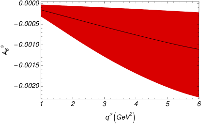
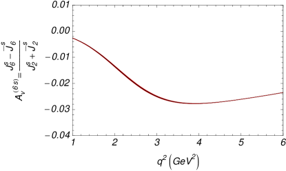
Figure 1: SM prediction of the CP violating observables $A_{6s}$ (left) and $A_{6s}^{V2s}$ (right) as function of the squared lepton mass with uncertainty due to the soft form factors only.

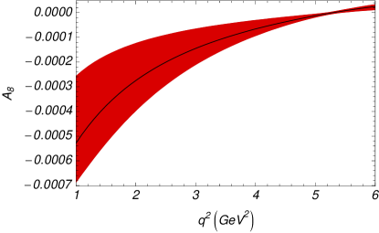
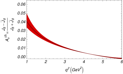
Figure 2: SM prediction of the CP violating observables $A_{8}$ (left) and $A_{8}^{V}$ (right) with uncertainty due to the soft form factors only.

The $J_{i}$ are bilinear in the $K^{*}$ spin amplitudes, so it is clear from the LO formulae (6) that -following the strategy of Ref.[10] - any form factor dependence at this order cancels out in both observables. We note that $J_{2s}$ has the same form factor dependence as $J_{6s}$ but has larger absolute values over the dilepton mass spectrum that stabilizes the quantity. In Fig. 1 the uncertainty due to the form factor dependence is estimated in a conservative way (for more details see Ref. [12]) for $A_{6s}$ defined in (11) and for $A_{6s}^{V}$ defined in (12). Comparing the plots, one sees that with the appropriate normalization this main source of hadronic uncertainties gets almost eliminated. The left-over uncertainty enters through the form factor dependence of the NLO contribution. Fig. 2 shows the analogous results for the observable $A_{8}^{V}$.

In the second step we try to make the possible $\mathchar 28931\relax/m_{b}$ corrections manifest in our final results. To explore the corresponding uncertainties we introduce a set of extra parameters for each spin amplitude:

$$A=A_{1}\times(1+C_{1}e^{i\phi_{1}})+e^{i\theta}A_{2}\times(1+C_{2}e^{i\phi_{2}}),$$ (13)

where $A_{1,2}$ are the relevant sub–amplitudes and $\theta$ is the weak phase. We assume that the subamplitudes can each receive a $\mathchar 28931\relax/m_{b}$ correction as well as an additional, currently unconstrained strong phase, $\phi_{1,2}$. For the absolute size of the corrections we use a dimensional estimate fixing $C_{1,2}$ to be of order $5-10\%$. To access the effects of these uncertainties on the individual observables, we form an ensemble of theory predictions, where each amplitude is randomly assigned values of $\phi_{1,2}$ and $C_{1,2}$ from a Uniform distribution over the specified ranges. It is assumed that the values of these parameters are not functions of $q^{2}$. This ensemble is used to calculate a 66% confidence band for each observable by looking at the spread of predictions for each observable at each point in $q^{2}$. The bands produced show the expected uncertainty on each observable given the estimated ranges for the unknown parameters.

Within the SM, we have only one weak phase and the two subamplitudes are contructed in the following way;

$$A=A_{\rm SM}(\lambda_{u}=0)\times(1+C_{1}e^{i\phi_{1}})+(A_{\rm SM}(\lambda_{u}\neq 0)-A_{\rm SM}(\lambda_{u}=0))\times(1+C_{2}e^{i\phi_{2}})$$ (14)

It turns out that in spite of this very conservative ansatz for the possible power corrections - we neglect for example any kind of correlations between such corrections in the various spin amplitudes - the impact of those corrections is smaller than the SM uncertainty in case of the two observables $A_{6s}^{V}$ and $A_{8}^{V}$. In the left plot of Fig. 3 the SM error is given including uncertainties due to the scale dependence and input parameters and the spurious error due to the form factors. In the right plot the estimated power corrections are given, which in case of the CP violating observable $A_{6s}^{V}$ are significantly smaller than the combined uncertainty due to scale and input parameters. Fig. 4 shows the same feature for the CP violating observable $A_{8}^{V}$. This result is in contrast to the one for CP-averaged angular observables discussed in Ref. [10], where the estimated power corrections always represent the dominant error. As the reason for this specific feature one identifies the smallness of the weak phase in the SM. Thus, one expects that the impact of power corrections will be significantly larger when NP scenarios with new CP phases are considered (see below).

In the third step we consider various NP scenarios. Here we follow the model-independent constraints derived in Ref. [15] assuming only one NP Wilson coefficient being nonzero. We consider three different NP benchmarks of this kind:

1. $|C_{9}^{\rm NP}|=2$. and $\Theta_{9}^{\rm NP}=\pi/8$

2. $|C_{10}^{\rm NP}|=1.5$. and $\Theta_{10}^{\rm NP}=\pi/8$

3. $|C^{{}^{\prime}}_{10}|=3$. and $\Theta_{10}^{{}^{\prime}}=\pi/8$

The absolute values are chosen in such a way that the model-independent analysis, assuming one nontrivial NP Wilson coefficient at a time, does not give any bound on the corresponding NP phase. Scenarios with larger phase values will be discussed in Ref. [12]. Fig. 5 shows that the CP violating observable $A_{6s}^{V}$ might separate a NP scenario (2), while the central values of scenarios (1) and (3) are very close to the SM. Moreover observable $A_{*}^{V}$ seems to be suited to separate scenarios (1) and (3) from the SM.

However, to judge the NP reach we need a complete error analysis within the three NP scenarios. Thus, let us consider the possible impact of unknown power corrections in these cases: With one new CP phase involved we work now with three weak subamplitudes in which possible power corrections are varied independently.

The left plots in Figs. 6 and 7 show that the possible $\mathchar 28931\relax/m_{b}$ corrections have a much larger impact than in the SM and become the dominating theoretical uncertainty. However, the two CP violating observables could discriminate the specific NP scenarios with new CP phase of order $\pi/8$ from the SM in view of the theoretical errors only.

In the last step, we analyse the experimental sensitivity of the angular CP asymmetries using a toy Monte Carlo model. The right plots in Figs. 6 and 7 show the estimates of the statistical uncertainty of $A_{6s}^{V}$ and $A_{8}^{V}$ with statistics corresponding to five years of nominal running at LHCb ($10fb^{-1}$). The inner and outer bands correspond to $1\sigma$ and $2\sigma$ statistical errors. The plots show that all the NP benchmarks are within the $1\sigma$ range of the expected experimental error in case of the observable $A_{6s}^{V}$, and within the $2\sigma$ range of the experimental error in case of the observable $A_{8}^{V}$.

Thus, our final conclusion is that while the prospects of NP discovery of the CP conserving observable presented in ref. [10] both from the theoretical and experimental point of view are excellent, the possibility to disentangle different NP scenarios for the CP violating observables remains rather difficult. For the studied observables, LHCb has no real sensitivity for NP phases up to values of $\pi/8$ in the Wilson coefficients $C_{9}$, $C_{10}$, and their chiral counterparts via the rare decays $\bar{B}\rightarrow\bar{K}^{*}\ell^{+}\ell^{-}$. Even Super-LHCb with $100fb^{-1}$ integrated luminosity does not improve the situation significantly.

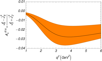
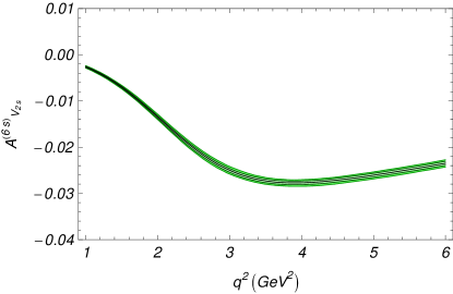
Figure 3: SM uncertainty in $A_{6s}^{V2s}$ (left) and estimate of uncertainty due to $\mathchar 28931\relax/m_{b}$ corrections with $C_{1,2}=10\%$ (right).

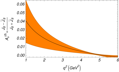
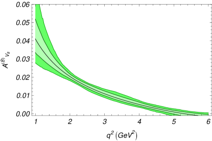
Figure 4: SM uncertainty in $A_{8}^{V}$ (left) and estimate of uncertainty due to $\mathchar 28931\relax/m_{b}$ corrections (right, light grey (green) corresponds to $C_{1,2}=5\%$, dark grey (green) to $C_{1,2}=10\%$).

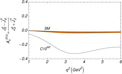
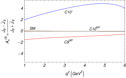
Figure 5: New physics scenarios, assuming one nontrivial NP Wilson coefficient at a time, next to SM prediction for $A_{6s}^{V2s}$ (left) and $A_{8}^{V}$ (right), for concrete values see text.

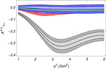
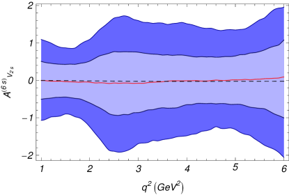
Figure 6: $A_{6s}^{V2s}$: Estimate of uncertainty due to $\mathchar 28931\relax/m_{b}$ corrections (left) and experimental uncertainty (right).

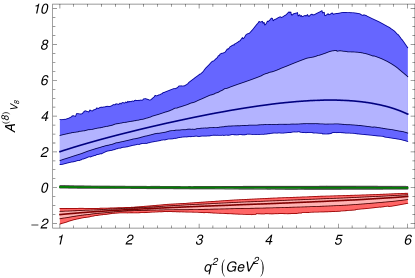
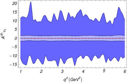
Figure 7: $A_{8}^{V}$: Estimate of uncertainty due to $\mathchar 28931\relax/m_{b}$ corrections (left) and experimental uncertainty (right).

References

- [1]
- [2]
- [3] http://www.slac.stanford.edu/BFROOT/
- [4] http://belle.kek.jp/
- [5] http://www-cdf.fnal.gov/physics/new/bottom/bottom.html
- [6] http://www-d0.fnal.gov/Run2Physics/ckm/
- [7] M. Artuso et al., Eur. Phys. J. C 57 (2008) 309 [arXiv:0801.1833 [hep-ph]].
- [8] M. Kobayashi and T. Maskawa, Prog. Theor. Phys. 49 (1973) 652.
- [9] http://nobelprize.org
- [10] U. Egede, T. Hurth, J. Matias, M. Ramon and W. Reece, arXiv:0807.2589 [hep-ph].
-
[11]
U. Egede, T. Hurth, J. Matias, M. Ramon and W. Reece,
talk at Flavianet Meeting
“The exclusive New ,” Kazimierz, July 2009, [arXiv:0912.1339 [hep-ph]]. - [12] U. Egede, T. Hurth, J. Matias, M. Ramon and W. Reece, in preparation.
- [13] F. Krüger, L. M. Sehgal, N. Sinha, and R. Sinha, Phys. Rev. 61 (2000) 114028; Phys. Rev. 63 (2001) 019901(E).
- [14] F. Krüger, Chapter 2.17 in J. L. . Hewett et al., “The discovery potential of a Super B Factory. Proceedings, SLAC Workshops, Stanford, USA, 2003,” arXiv:hep-ph/0503261.
- [15] C. Bobeth, G. Hiller and G. Piranishvili, JHEP 0807 (2008) 106 [arXiv:0805.2525 [hep-ph]].
- [16] M. Beneke, T. Feldmann and D. Seidel, Nucl. Phys. B 612 (2001) 25 [arXiv:hep-ph/0106067].
- [17] M. Beneke, T. Feldmann and D. Seidel, Eur. Phys. J. C 41 (2005) 173 [arXiv:hep-ph/0412400].
- [18] J. Charles, A. Le Yaouanc, L. Oliver, O. Pene and J. C. Raynal, Phys. Rev. D 60 (1999) 014001 [arXiv:hep-ph/9812358].
- [19] M. Beneke and T. Feldmann, Nucl. Phys. B 592 (2001) 3 [arXiv:hep-ph/0008255].
- [20] G. Buchalla, G. Hiller and G. Isidori, Phys. Rev. D 63, 014015 (2000) [arXiv:hep-ph/0006136].
- [21] F. Kruger and E. Lunghi, Phys. Rev. D 63, 014013 (2001) [arXiv:hep-ph/0008210].
- [22] W. Altmannshofer, P. Ball, A. Bharucha, A. J. Buras, D. M. Straub and M. Wick, JHEP 0901 (2009) 019 [arXiv:0811.1214 [hep-ph]].
- [23]