A fast algorithm for the linear canonical transform

MSC: 65T50; 44A15; 65D32
Keywords: Linear Canonical Transform, Fractional Fourier Transform, Quadrature, Hermite polynomials, Fractional Discrete Fourier Transform, fft

Abstract

In recent years there has been a renewed interest in finding fast algorithms to compute accurately the linear canonical transform (LCT) of a given function. This is driven by the large number of applications of the LCT in optics and signal processing. The well-known integral transforms: Fourier, fractional Fourier, bilateral Laplace and Fresnel transforms are special cases of the LCT. In this paper we obtain an ${\mathcal{O}}(N\log N)$ algorithm to compute the LCT by using a chirp-FFT-chirp transformation yielded by a convergent quadrature formula for the fractional Fourier transform. This formula gives a unitary discrete LCT in closed form. In the case of the fractional Fourier transform the algorithm computes this transform for arbitrary complex values inside the unitary circle and not only at the boundary. In the case of the ordinary Fourier transform the algorithm improves the output of the FFT.

1 Introduction

The Linear Canonical Transform (LCT) of a given function $f(x)$ is a three-parameter integral transform that was obtained in connection with canonical transformations in Quantum Mechanics [1, 2]. It is defined by

$${\mathcal{L}}^{\{a,b,c,d\}}[f(x),y] = \frac{1}{\sqrt{2\pi ib}}\int_{-\infty}^{\infty}e^{\frac{i}{2b}(ax^{2}-2xy+dy^{2})}f(x)dx,$$

for $b\neq 0$, and by $\sqrt{d}e^{\frac{i}{2}cdy^{2}}f(dy)$, if $b=0$. The four parameters $a$, $b$, $c$ and $d$ appearing in (1), are the elements of a $2\times 2$ matrix with unit determinant, i.e., $ad-bc=1$. Therefore, only three parameters are free. Since this transform is a useful tool for signal processing and optical analysis, its study and direct computation in digital computers has become an important issue [3]-[10], particularly, fast algorithms to compute the linear canonical transform have been devised [4, 7]. These algorithms use the following related ideas: (a) use of the periodicity and shifting properties of the discrete LCT to break down the original matrix into smaller matrices as the FFT does with the DFT, (b) decomposition of the LCT into a chirp-FFT-scaling transformation and (c) decomposition of the LCT into a fractional Fourier transform followed by a scaling-chirp multiplication. All of these are algorithms of ${\mathcal{O}}(N\log N)$ complexity.
In this paper we present an algorithm that takes ${\mathcal{O}}(N\log N)$ time based in the decomposition of the LCT into a scaling-chirp-DFT-chirp-scaling transformation, obtained by using a quadrature formula of the continuous Fourier transform [11, 12]. Here, DFT stands for the standard discrete Fourier transform. To distinguish this discretization from other implementations, we call it the extended Fourier Transform (XFT). Thus, the quadrature from which the XFT is obtained, uses some asymptotic properties of the Hermite polynomials and yields a fast algorithm to compute the Fourier transform, the fractional Fourier transform and therefore, the LCT. The quadrature formula is ${\mathcal{O}}(1/N)$-convergent to the continuous Fourier transform for certain class of functions [13].

2 A discrete fractional Fourier transform

In previous work [12], [13], [14], we derived a quadrature formula for the continuous Fourier transform which yields an accurate discrete Fourier transform. For the sake of completeness we give in this section a brief review of the main steps to obtain this formula.
Let us consider the family of Hermite polynomials $H_{n}(x)$, $n=0,1,\ldots$, which satisfies the recurrence equation

$$H_{n+1}(x)+2nH_{n-1}(x)=2xH_{n}(x),$$ (1)

with $H_{-1}(x)\equiv 0$. Note that the recurrence equation (1) can be written as the eigenvalue problem

$$\begin{pmatrix}0&1/2&0&\cdots\\ 1&0&1/2&\cdots\\ 0&2&0&\cdots\\ \vdots&\vdots&\vdots&\ddots\\ \end{pmatrix}\begin{pmatrix}H_{0}(x)\\ H_{1}(x)\\ H_{2}(x)\\ \vdots\end{pmatrix}=x\begin{pmatrix}H_{0}(x)\\ H_{1}(x)\\ H_{2}(x)\\ \vdots\end{pmatrix}.$$ (2)

Let us now consider the eigenproblem associated to the principal submatrix of dimension $N$ of (2)

$${\mathcal{H}}=\begin{pmatrix}0&1/2&0&\cdots&0&0\\ 1&0&1/2&\cdots&0&0\\ 0&2&0&\cdots&0&0\\ \vdots&\vdots&\vdots&\ddots&\vdots&\vdots\\ 0&0&0&\cdots&0&1/2\\ 0&0&0&\cdots&N-1&0\end{pmatrix}.$$

It is convenient to symmetrize ${\mathcal{H}}$ by using the similarity transformation $S{\mathcal{H}}S^{-1}$ where $S$ is the diagonal matrix

$$S=\text{diag}\left\{1,\frac{1}{\sqrt{2}},\ldots,\frac{1}{\sqrt{(N-1)!\,2^{N-1}}}\right\}.$$

Thus, the symmetric matrix $H=S{\mathcal{H}}S^{-1}$ takes the form

$$\begin{pmatrix}0&\sqrt{\frac{1}{2}}&0&\cdots&0&0\\ \sqrt{\frac{1}{2}}&0&\sqrt{\frac{2}{2}}&\cdots&0&0\\ 0&\sqrt{\frac{2}{2}}&0&\cdots&0&0\\ \vdots&\vdots&\vdots&\ddots&\vdots&\vdots\\ 0&0&0&\cdots&0&\sqrt{\frac{N-1}{2}}\\ 0&0&0&\cdots&\sqrt{\frac{N-1}{2}}&0\end{pmatrix}.$$

The recurrence equation (1) and the Christoffel-Darboux formula [15] can be used to solve the eigenproblem

$$Hu_{k}=x_{k}u_{k},\quad k=1,2,\ldots,N,$$

which is a finite-dimensional version of (2). The eigenvalues $x_{k}$ are the zeros of $H_{N}(x)$ and the $k$th eigenvector $u_{k}$ is given by

$$c_{k}\left(s_{1}H_{0}(x_{k}),s_{2}H_{1}(x_{k}),\cdots,s_{N}H_{N-1}(x_{k})\right)^{T},$$

where $s_{1},\ldots,s_{N}$ are the diagonal elements of $S$ and $c_{k}$ is a normalization constant that can be determined from the condition $u_{k}^{T}\,u_{k}=1$, i.e., from

$$c_{k}^{2}\,\sum_{n=0}^{N-1}\frac{H_{n}(x_{k})H_{n}(x_{k})}{2^{n}n!}=1.$$

Therefore,

$$c_{k}=\sqrt{\frac{2^{N-1}\,(N-1)!}{N}}\,\frac{(-1)^{N+k}}{H_{N-1}(x_{k})}.$$

Thus, the components of the orthonormal vectors $u_{k}$, $k=1,2,\ldots,N$, are

$$(u_{k})_{n}=(-1)^{N+k}\sqrt{\frac{2^{N-n}\,(N-1)!}{N\,(n-1)!}}\,\frac{H_{n-1}(x_{k})}{H_{N-1}(x_{k})},$$ (3)

$n=1,\ldots,N$. Let $U$ be the orthogonal matrix whose $k$th column is $u_{k}$ and let us define the matrix

$${\mathcal{F}}_{z}=\sqrt{2\pi}U^{-1}D(z)U,$$

where $D(z)$ is the diagonal matrix $D(z)=\text{diag}\{1,z,z^{2},\ldots,z^{N-1}\}$ and $z$ is an complex number. Therefore, the components of ${\mathcal{F}}_{z}$ are given by

$$({\mathcal{F}}_{z})_{jk} = \sqrt{2\pi}\,\frac{(-1)^{j+k}\,2^{N-1}\,(N-1)!}{N\,H_{N-1}(x_{j})H_{N-1}(x_{k})}\sum_{n=0}^{N-1}\frac{z^{n}}{2^{n}\,n!}H_{n}(x_{j})H_{n}(x_{k}).$$ (4)

Next, we want to prove that if $N$ is large enough, (4) approaches the kernel of the fractional Fourier transform evaluated at $x=x_{j}$, $y=x_{k}$. To this, we use the asymptotic expression for $H_{N}(x)$ [15])

$$H_{N}(x)\simeq\frac{\Gamma(N+1)e^{x^{2}/2}}{\Gamma(N/2+1)}\cos(\sqrt{2N+1}\,\,x-\frac{N\pi}{2}).$$ (5)

Thus, the asymptotic form of the zeros of $H_{N}(x)$ are

$$x_{k}=\left(\frac{2k-N-1}{\sqrt{2N}}\right)\frac{\pi}{2},$$ (6)

$k=1,2,\ldots,N$. The use of (5) and (6) yields

$$H_{N-1}(x_{k})\simeq(-1)^{N+k}\,\frac{\Gamma(N)}{\Gamma(\frac{N+1}{2})}\,e^{x_{k}^{2}/2},\quad N\to\infty,$$

and the substitution of this asymptotic expression in (4) yields

$$({\mathcal{F}}_{z})_{jk} \simeq \sqrt{2\pi}\,\frac{2^{N-1}\,[\Gamma(\frac{N+1}{2})]^{2}}{\Gamma(N+1)}\,\,e^{-(x_{j}^{2}+x_{k}^{2})/2}\sum_{n=0}^{\infty}\frac{z^{n}}{2^{n}\,n!}H_{n}(x_{j})H_{n}(x_{k}).$$

Finally, Stirling’s formula and Mehler’s formula [16] produce

$$({\mathcal{F}}_{z})_{jk}\simeq\sqrt{\frac{2}{1-z^{2}}}\,e^{-\frac{(1+z^{2})(x_{j}^{2}+x_{k}^{2})-4x_{j}x_{k}z}{2(1-z^{2})}}\Delta x_{k},$$ (7)

where $\Delta x_{k}$ is the difference between two consecutive asymptotic Hermite zeros, i.e.,

$$\Delta x_{k}=x_{k+1}-x_{k}=\frac{\pi}{\sqrt{2N}}.$$ (8)

Let us consider now the vector of samples of a given function $f(x)$

$$f=(f(x_{1}),f(x_{2}),\ldots,f(x_{N}))^{T}.$$

The multiplication of the matrix ${\mathcal{F}}_{z}$ by the vector $f$ gives the vector $g$ with entries

$$g_{j} = \sum_{k=1}^{N}({\mathcal{F}}_{z})_{jk}f(x_{k})\simeq\sqrt{\frac{2}{1-z^{2}}}\sum_{k=1}^{N}e^{-\frac{(1+z^{2})(x_{j}^{2}+x_{k}^{2})-4x_{j}x_{k}z}{2(1-z^{2})}}f(x_{k})\Delta x_{k},$$

where $j=1,2\ldots,N.$ This equation is a Riemann sum for the integral

$${\mathscr{F}}_{z}[f(x),y] = \sqrt{\frac{2}{1-z^{2}}}\int_{-\infty}^{\infty}e^{-\frac{(1+z^{2})(y^{2}+x^{2})-4xyz}{2(1-z^{2})}}f(x)dx,$$

where $|z|<1$. Therefore, if we make $y_{j}=x_{j}$,

$${\mathscr{F}}_{z}[f(x),y_{j}]\simeq\sum_{k=1}^{N}({\mathcal{F}}_{z})_{jk}f(x_{k}),\quad N\to\infty.$$ (9)

Note that ${\mathscr{F}}_{z}[g(x),y]$ is the continuous fractional Fourier transform [17] of $g(x)$ except for a constant and therefore, ${\mathcal{F}}_{z}$ is a discrete fractional Fourier transform.

3 A fast linear canonical transform

Firstly, note that if $b\neq 0$, the LCT can be written as a chirp-FT-chirp transform

$${\mathcal{L}}^{\{a,b,c,d\}}[f(x),y] = \frac{e^{\frac{idy^{2}}{2b}}}{\sqrt{2\pi ib}}\int_{-\infty}^{\infty}e^{-\frac{ixy}{b}}e^{\frac{iax^{2}}{2b}}f(x)dx.$$

Thus, for $b\neq 0$, the LCT of the function $f(x)$ can be represented by the $1/b$-scaled Fourier transform of the function $g(x)=e^{\frac{iax^{2}}{2b}}f(x)$, multiplied by $\frac{e^{\frac{idy^{2}}{2b}}}{\sqrt{2\pi ib}}$.
On the other hand, note that for the case $z=\pm i$, (7) yields a discrete Fourier transform $({\mathcal{F}}_{\pm i})_{jk}\simeq e^{\pm it_{j}t_{k}}\Delta t_{k}$, that can be related to the standard DFT as follows. The use of (6) yields

$$({\mathcal{F}}_{i})_{jk}=e^{\pm it_{j}t_{k}}\Delta t_{k}=\frac{\pi}{\sqrt{2N}}e^{i\frac{\pi^{2}}{2N}\left(j-\frac{N-1}{2}\right)\left(k-\frac{N-1}{2}\right)}$$ (10)

where we have used (6) and (8). Since $\sum_{k=1}^{N}({\mathcal{F}}_{i})_{jk}f(x_{k})$ is a quadrature and therefore, an approximation of

$$g(y_{j})=\int_{-\infty}^{\infty}e^{iy_{j}x}f(x)dx,$$

a scaled Fourier transform

$$\int_{-\infty}^{\infty}e^{i\kappa y_{j}x}f(x)dt=g(\kappa y_{j})$$ (11)

has the quadrature $\sum_{k=1}^{N}\tilde{F}_{jk}f(x_{k})$, where

$$\tilde{F}_{jk}=\frac{\pi}{\sqrt{2N}}e^{i\kappa\frac{\pi^{2}}{2N}\left(j-\frac{N-1}{2}\right)\left(k-\frac{N-1}{2}\right)}.$$ (12)

If we choose $\kappa=4/\pi$, (12) takes the form

$$F_{jk} = \frac{\pi e^{i\frac{\pi}{2}\frac{(N-1)^{2}}{N}}}{\sqrt{2N}}\left[e^{-i\pi\frac{N-1}{N}j}\right]\left[e^{i\frac{2\pi}{N}jk}\right]\left[e^{-i\pi\frac{N-1}{N}k}\right],$$

for $j,k=0,1,2,\ldots,N-1$, and $\sum_{k=1}^{N}F_{jk}f(x_{k})$ is an approximation of $g(4y_{j}/\pi)$. If now we choose $\kappa=4b/\pi$, but we keep the same matrix (3), then $\sum_{k=1}^{N}F_{jk}f(x_{k})$ is an approximation of

$$\int_{-\infty}^{\infty}e^{i\frac{y_{j}}{b}x}f(x)dt.$$

If now we replace $f(x)$ by $e^{\frac{iax^{2}}{2b}}f(x)$ and take into account (3), we have that

$$\sum_{k=1}^{N}F_{jk}e^{iax_{k}^{2}/2b}f(x_{k})$$

is an approximation of the product of functions $\left(\frac{e^{\frac{idy^{2}}{2b}}}{\sqrt{2\pi ib}}\right)^{-1}{\mathcal{L}}^{\{a,b,c,d\}}[f(x),y]$ evaluated at $y_{j}=4bx_{j}/\pi$. Therefore, a discrete (scaled) linear canonical transform $L$ can be given in closed form. If we denote by $G(y)$ the LCT of $f(x)$, then

$$G(y_{j})=G(4bx_{j}/\pi)=\sum_{k=1}^{N}(S_{1}FS_{2})_{jk}f(x_{k}),$$

where $S_{1}$ and $S_{2}$ are diagonal matrices whose diagonal elements are $e^{\frac{idy_{j}^{2}}{2b}}/\sqrt{2\pi ib}$, and $e^{iax_{j}^{2}/2b}$, respectively. As it can be seen, the matrix $L=S_{1}FS_{2}$, which gives the discrete LTC, i.e., the XFT, consists in a chirp-DFT-chirp transformation, where DFT stands for the standard discrete Fourier transform. Therefore, we can use any FFT to give a fast computation of the linear canonical transform $G=Lf$.
Now, the fast algorithm for the linear canonical transform can be given straightforwardly.

Algorithm  To compute an approximation $G=(G_{1},G_{2},\ldots,G_{N})^{T}$ of the linear canonical transform $G(y)={\mathcal{L}}^{\{a,b,c,d\}}[f(x),y]$ evaluated at $y_{j}=4bx_{j}/\pi$, where $x_{j}=\left(\frac{2j-N-1}{\sqrt{2N}}\right)\frac{\pi}{2}$. 1. For given $N$ set up the vector $u$ of components $\displaystyle u_{k}$ $\displaystyle=$ $\displaystyle e^{-i\pi\frac{(k-1)(N-1)}{N}}e^{iax_{k}^{2}/2b}f\left(\pi\frac{2k-N-1}{2\sqrt{2N}}\right),$ $k=1,2,\ldots,N$. 2. Set $y_{j}=4bx_{j}/\pi$ and compute the diagonal matrix $S$ according to $$S_{jk}=\frac{\pi e^{i\frac{\pi}{2}\frac{(N-1)^{2}}{N}}}{\sqrt{2N}}\frac{e^{\frac{idy_{j}^{2}}{2b}}e^{-i\pi\frac{N-1}{N}(j-1)}}{\sqrt{2\pi ib}}\delta_{jk},$$ $j,k=1,2,\ldots,N$. 3. Let $D_{F}$ be the discrete Fourier transform, i.e., $(D_{F})_{jk}=e^{i\frac{2\pi}{N}jk}$, $j,k=0,1,2,\ldots,N-1$. Obtain the approximation $G_{j}$ to $G(\frac{4b}{\pi}x_{j})$ by computing the matrix-vector product $$G=SD_{F}u,$$ (13) with a standard FFT algorithm.

4 Example

For this example we take an integral formula found in [18] that gives

$$G(y) = \frac{\sqrt{\pi}}{\sqrt{2\pi ib}(\alpha^{2}+\frac{a^{2}}{4b^{2}})^{1/4}}e^{\frac{\alpha(\beta^{2}-\alpha\gamma)}{\alpha^{2}+\frac{a^{2}}{4b^{2}}}}e^{\frac{i}{2}\arctan(\frac{a}{2\alpha b})}e^{-\frac{\alpha y^{2}+2\beta ay+a^{2}\gamma}{4b^{2}\alpha^{2}+a^{2}}}$$

$$\times e^{i\frac{acy^{2}}{2(4b^{2}\alpha^{2}+a^{2})}}e^{i\frac{2b(\alpha^{2}dy^{2}+2\beta\alpha y+\beta^{2}a)}{4b^{2}\alpha^{2}+a^{2}}},$$

if $f(x)=e^{-(\alpha y^{2}+2\beta y+\gamma)}$, $\alpha>0$. Figure 1 shows the exact LTC with $\alpha=1$, $\beta=2$, $\gamma=3$, $a=1$, $b=2$, $c=1/2$, and $d=2$, compared with the approximation given by the XFT.

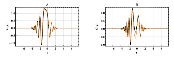
Figure 1: Real part (A) and imaginary part (B) of the exact linear canonical transform (solid line) compared with the output of the XFT (dashed line) computed with $N=512$. The function $G(y)$ is that given in (4) for $\alpha=1$, $\beta=2$, $\gamma=3$, $a=1$, $b=2$, $c=1/2$, and $d=2$.

Figure 2 shows the exact Fresnel transform of $f(x)=e^{-(\alpha y^{2}+2\beta y+\gamma)}$ with $\alpha=2$, $\beta=1$, $\gamma=3$, $a=1$, $b=100$, $c=0$, and $d=1$, compared with the approximation given by the XFT.

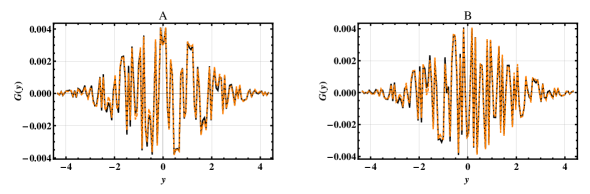
Figure 2: Real part (A) and imaginary part (B) of the exact Fresnel transform (solid line) compared with the output of the XFT (dashed line) computed with $N=1024$. The function $G(y)$ is that given in (4) for $\alpha=2$, $\beta=1$, $\gamma=3$, $a=1$, $b=100$, $c=0$, and $d=1$.

5 Conclusion

We have obtained a discrete linear canonical transform and a fast algorithm to compute this transform by projecting the space of functions onto a vector space spanned by a finite number of Hermite functions. The XFT is a discrete LCT given by a unitary matrix in a closed form in which the DFT can be found at the core, surrounded by diagonal transformations, which makes easy to implement it in a fast algorithm. Since this discrete LCT is related to a quadrature formula of the fractional Fourier transform, it yields accurate results.

References

• [1] M. Moshinsky and C. Quesne, โ€œLinear Canonical Transformations and their unitary representations,โ€ J. Math. Phys., vol.ย 12, pp. 1772-1783, 1971.
• [2] K.B Wolf, Integral Transforms in Science and Engineering, Ch. 9-10ย ย ย New York: Plenum Press, 1979.
• [3] J.J.Healy, J.T.Sheridan, โ€œSampling and discretization of the linear canonical transform,โ€ Signal Processing, vol.ย 89, pp. 641-648, 2009.
• [4] A. Koรง, H.M. Ozaktas, C. Candan, M.A. Kutay, โ€œDigital Computation of Linear Canonical Transforms,โ€ IEEE Trans. Sig. Proc., vol.ย 56, pp. 2383-2394, 2008.
• [5] K.K.Sharma, S.D. Joshi, โ€œUncertainty Principle for Real Signals in the Linear Canonical Transform Domains,โ€ IEEE Trans. Sig. Proc., vol.ย 56, pp. 2677-2683, 2008.
• [6] A. Stern, โ€œSampling of linear canonical transformed signals,โ€ Signal Processing, vol.ย 86, pp. 1421-1425, 2006.
• [7] B.M. Hennelly, J.T. Sheridan, โ€œFast numerical algorithm for the linear canonical transform,โ€ J. Opt. Soc. Am., vol.ย A22, pp. 928-937, 2005.
• [8] B.M. Hennelly, J.T. Sheridan, โ€œGeneralizing, optimizing, and inventing numerical algorithms for the fractional Fourier, Fresnel, and linear canonical transforms,โ€ J. Opt. Soc. Am., vol.ย A22, pp. 917-927, 2005.
• [9] B.Z. Li, R. Tao, Y. Wang, โ€œNew sampling formulae related to linear canonical transform,โ€ Signal Processing, vol.ย 87, pp. 983-990, 2007.
• [10] S.C. Pei, J.J. Ding, โ€œEigenfunctions of Linear Canonical Transform,โ€ IEEE Trans. Sig. Proc., vol.ย 50, pp. 11-26, 2002.
• [11] R.G. Campos, J. Rico-Melgoza, E. Chรกvez, โ€œRFT: A fast discrete fractional Fourier transform,โ€ unpublished.
• [12] R. G. Campos, and L.Z. Juรกrez, โ€œA discretization of the Continuous Fourier Transformโ€, Il Nuovo Cimento, vol.ย 107B, pp. 703-711, 1992.
• [13] R.G. Campos, โ€œA Quadrature Formula for the Hankel Transform,โ€ Numerical Algorithms, vol.ย 9, pp. 343-354, 1995.
• [14] R. G. Campos, F. Domรญnguez Mota and E. Coronado, โ€œQuadrature formulas for integrals transforms generated by orthogonal polynomials,โ€ arXiv.0805.2111v1 [math.NA].
• [15] G.ย Szego, Orthogonal Polynomials.ย ย ย Providence, Rhode Island: Colloquium Publications, American Mathematical Society, 1975.
• [16] A.ย Erdรฉlyi, Higher Transcendental Functions. Vols. I and II.ย ย ย New York: McGraw Hill, 1953.
• [17] V.ย Namias, โ€œThe Fractional Order Fourier Transform and its Application to Quantum Mechanics,โ€ J. Inst. Maths. Applics., vol.ย 25, pp. 241โ€“265, 1980.
• [18] I.S. Gradshteyn, I.M. Ryzhik, Table of Integrals, Series and Products, Fifth editionย ย ย New York: Academic Press, 1994, p. 520.