KUNS-2245 RIKEN-TH-179 December 2009

Large $N$ reduction on group manifolds

Hikaru Kawai^1),2), Shinji Shimasaki¹⁾ and Asato Tsuchiya³⁾

¹⁾ Department of Physics, Kyoto University, Kyoto 606-8502, Japan
²⁾ Theoretical Physics Laboratory, RIKEN, Wako 351-0198, Japan
³⁾ Department of Physics, Shizuoka University
836 Ohya, Suruga-ku, Shizuoka 422-8529, Japan

We show that the large $N$ reduction holds on group manifolds. Large $N$ field theories defined on group manifolds are equivalent to some corresponding matrix models. For instance, gauge theories on $S^{3}$ can be regularized in a gauge invariant and $SO(4)$ invariant manner.

1 Introduction

It has been widely recognized that space-time can be emergent from the degrees of freedom of matrices. Such emergent space-time was first observed in the large $N$ reduction [1] (for further developments, see [2, 3, 4, 5, 6, 7, 8, 9, 10, 11, 12]). It asserts that the planar (’t Hooft) limit of gauge theories can be described by the matrix models obtained by the dimensional reduction to lower (zero) dimensions. These matrix models are called the (large $N$) reduced models. The large $N$ reduction has been studied so far on flat space-time, except for a few cases. It would be important to investigate whether it also holds on curved space-times. This is because it would provide insight into the description of curved space-times [13] in the matrix models [14, 15] that are conjectured to give a nonperturbative formulation of string theory and take the form of the reduced model of ten-dimensional ${\cal N}=1$ super Yang-Mils theory (SYM). Practically, it can also be applied to a nonperturbative regularization of planar gauge theories on curved space-time.

In this paper, we show that the large $N$ reduction holds on group manifolds, which are typical examples of curved spaces. In the literature, the mechanism of the large $N$ reduction is usually explained in the momentum space. Here we first review it in the real space. We see that the reduced model can be viewed as a bi-local field theory with a special feature. This point of view makes it easy to generalize the large $N$ reduction on flat space to that on group manifolds. We study the large $N$ reduction for scalar theories in detail. It turns out that the generalization to gauge theories is straightforward. As an example, we describe the large $N$ reduction for ${\cal N}=4$ SYM on $R\times S^{3}$. We discuss a relation of a recently proposed large $N$ reduction for ${\cal N}=4$ SYM on $R\times S^{3}$ [16] with our version. We also discuss the large $N$ reduction on coset spaces.

This paper is organized as follows. In section 2, we review the large $N$ reduction for scalar theories on flat space. We show that the large $N$ reduction holds for the scalar theories on group manifolds in section 3, and for gauge theories on group manifolds in section 4. In section 5, the results in sections 3 and 4 are applied to ${\cal N}=4$ SYM on $R\times S^{3}$. Section 6 is devoted to summary and discussion.

2 Large $N$ reduction on flat space

To illustrate the large $N$ reduction [1] on flat space, we consider the scalar $\phi^{3}$ theory on $R^{d}$. The action is given by

$$S=\int d^{d}x\ \mathrm{Tr}\left(\frac{1}{2}(\partial_{\mu}\phi(x))^{2}+\frac{1}{2}m^{2}\phi(x)^{2}+\frac{1}{3}\kappa\phi(x)^{3}\right),$$ (2.1)

where $\phi(x)$ is an $N\times N$ hermitian matrix. We take the planar (’t Hooft) limit in which

$$N\rightarrow\infty,\;\;\kappa\rightarrow 0\;\;\;\mbox{with}\;\;\kappa^{2}N=\lambda\;\;\mbox{fixed},$$ (2.2)

where $\lambda$ is the ’t Hooft coupling.

The propagator takes the form

$$\langle\phi(x_{1})_{ij}\phi(x_{2})_{kl}\rangle=D(x_{1}-x_{2})\delta_{il}\delta_{jk}.$$ (2.3)

The detailed form of $D(x)$ is irrelevant in our argument. As an example, we calculate the free energy at the two-loop level. There are two 1PI diagrams depicted in Fig. 1 and Fig. 2. The diagram in Fig. 1 is planar while the one in Fig. 2 is non-planar. The result of the planar diagram in Fig. 1 is

$$\mbox{Fig. 1}=\frac{1}{6}N^{2}\lambda\int d^{d}x_{1}d^{d}x_{2}\ D(x_{1}-x_{2})^{3}.$$ (2.4)

The result of the non-planar diagram in Fig. 2 equals that in Fig. 1 divided by $N^{2}$. This is an illustration of the well-known fact that only the planar contribution survives in the large $N$ limit.

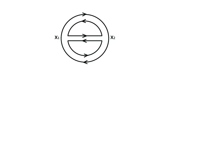
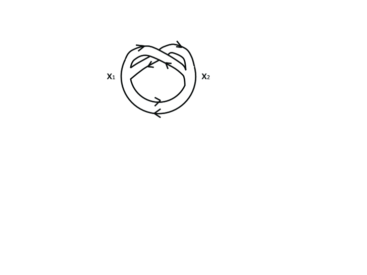
Figure 1: A planar diagram for the free energy of the scalar $\phi^{3}$ theory

Figure 2: A non-planar diagram for the free energy of the scalar $\phi^{3}$ theory

In order to define the reduced model of (2.1), we consider the space of functions on $R^{d}$. The rule to obtain the reduced model is given by

$$\phi(x)\rightarrow\hat{\phi},\;\;\;\partial_{\mu}\rightarrow[i\hat{P}_{\mu},\;],\;\;\;\int d^{d}x\rightarrow v,$$ (2.5)

where $\hat{\phi}$ is a hermitian operator acting on the space of function on $R^{d}$, and $\hat{P}_{\mu}$ is the momentum operator which acts on the coordinate basis $|x\rangle\ (x\in R^{d})$ as

$$\hat{P}_{\mu}|x\rangle=-\frac{1}{i}\frac{\partial}{\partial x^{\mu}}|x\rangle,\;\;\;\;\;\langle x|\hat{P}_{\mu}=\frac{1}{i}\frac{\partial}{\partial x^{\mu}}\langle x|.$$ (2.6)

$v$ is a parameter to be determined later. Then, by applying (2.5) to (2.1), we obtain the reduced model

$$S_{r}=v\mathrm{Tr}\left(\frac{1}{2}[i\hat{P}_{\mu},\hat{\phi}]^{2}+\frac{1}{2}m^{2}\hat{\phi}^{2}+\frac{1}{3}\kappa\hat{\phi}^{3}\right),$$ (2.7)

where $\mathrm{Tr}$ is the trace taken over the space of functions on $R^{d}$. (2.7) may look different from the reduced model. However, it reduces to the familiar form if one introduces a momentum cutoff $\Lambda$ and truncates the space of functions on $R^{d}$ to an $N$-dimensional vector space. Here we set

$$v=\left(\frac{2\pi}{\Lambda}\right)^{d},$$ (2.8)

and take a basis which diagonalizes $\hat{P}_{\mu}$. Then, $\hat{\phi}$ becomes an $N\times N$ hermitian matrix, and $\hat{P}_{\mu}$ become constant diagonal matrices whose eigenvalues distribute uniformly in a box defined by $-\Lambda/2\leq p_{\mu}\leq\Lambda/2$ in the $d$-dimensional momentum space. $\mathrm{Tr}$ is viewed as the trace over $N\times N$ matrices. The introduction of $\Lambda$ and $N$ is interpreted in the real space as follows. The real space is coarse grained to $N$ $d$-dimensional cubic cells with size $2\pi/\Lambda$. This indicates that the volume of the real space is given by $V=Nv$.

We reinterpret the large $N$ reduction in the real space, which makes it easy to generalize the large $N$ reduction on flat space to that on group manifolds. We denote the matrix element of $\hat{\phi}$ in the coordinate basis by $\langle x|\hat{\phi}|x^{\prime}\rangle\equiv\phi(x,x^{\prime})$, which is a bi-local field on $R^{d}$. The hermiticity of $\hat{\phi}$ requires that $\phi^{*}(x,x^{\prime})=\phi(x^{\prime},x)$. Using (2.6), we express (2.7) in the coordinate basis as

$$S_{r} =v\int d^{d}xd^{d}x^{\prime}\left(-\frac{1}{2}\phi(x^{\prime},x)\left(\frac{\partial}{\partial x^{\mu}}+\frac{\partial}{\partial{x^{\prime}}^{\mu}}\right)^{2}\phi(x,x^{\prime})+\frac{1}{2}m^{2}\phi(x^{\prime},x)\phi(x,x^{\prime})\right)$$

$$\qquad+v\int d^{d}xd^{d}x^{\prime}d^{d}x^{\prime\prime}\ \frac{1}{3}\kappa_{r}\phi(x,x^{\prime})\phi(x^{\prime},x^{\prime\prime})\phi(x^{\prime\prime},x).$$ (2.9)

Thus the reduced model can be viewed as a bi-local field theory. We make a change of variables given by

$$X^{\mu}=x^{\mu},\;\;\xi^{\mu}=x^{\mu}-x^{\prime}{}^{\mu},$$ (2.10)

and regard $\phi(x,x^{\prime})$ as a function of $X$ and $\xi$. $X^{\mu}$ are coordinates of one of the two end-points and $\xi^{\mu}$ are relative coordinates of the two end-points. Then, we obtain an equality

$$\left(\frac{\partial}{\partial x^{\mu}}+\frac{\partial}{\partial{x^{\prime}}^{\mu}}\right)\phi(x,x^{\prime})=\frac{\partial}{\partial X^{\mu}}\phi(x,x^{\prime}).$$ (2.11)

We see from the equality that the propagator in the reduced model takes the form

$$\langle\phi(x_{1},x_{1}^{\prime})\phi(x_{2}^{\prime},x_{2})\rangle=\frac{1}{v}D(x_{1}-x_{2})\delta^{d}((x_{1}-x_{1}^{\prime})-(x_{2}-x_{2}^{\prime})).$$ (2.12)

Each end-point propagates as a particle in the original field theory (2.1), while the relative coordinates are conserved during the propagation. This implies that

$$x_{1}-x_{2}=x_{1}^{\prime}-x_{2}^{\prime}$$ (2.13)

in the propagation, which also follows from the delta function in (2.12). In other words, the two end-points are parallely transported.

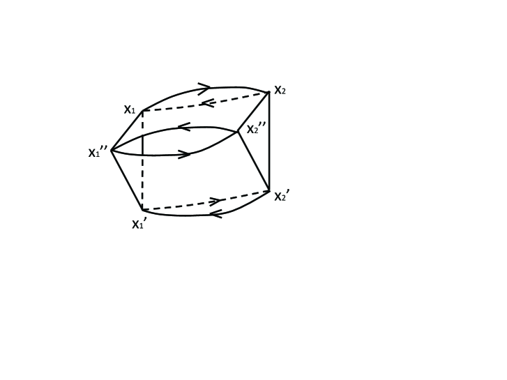
Figure 3: A planar diagram for the free energy of the reduced model.

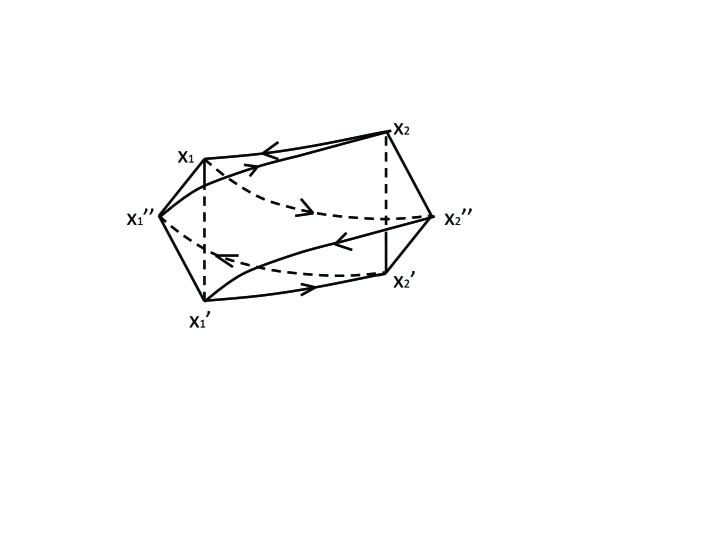
Figure 4: A non-planar diagram for the free energy of the reduced model.

Each diagram in the reduced model has the counterpart in the field theory, and vice versa. As an example, we calculate the free energy of the reduced model at the two-loop level again. The diagrams in Fig. 3 and Fig. 4 are the counterparts of the diagrams in Fig. 1 and Fig. 2, respectively. In Figs. 3 and 4, the aforementioned property of the propagator is visualized. Here the diagrams in the reduced model that are the counterparts of the planar diagrams in the field theory are still called the planar diagrams, although they can no longer be drawn on plane. Similarly, the diagrams in the reduced model that are the counterparts of the non-planar diagrams in the field theory are called the non-planar diagrams.

The calculation of the diagram in Fig. 3 is as follows:

$$\mbox{Fig. 3}= \frac{\kappa^{2}}{6v}\int d^{d}x_{1}d^{d}x_{1}^{\prime}d^{d}x_{1}^{\prime\prime}d^{d}x_{2}d^{d}x_{2}^{\prime}d^{d}x_{2}^{\prime\prime}\ D(x_{1}-x_{2})\delta^{d}((x_{1}-x_{1}^{\prime})-(x_{2}-x_{2}^{\prime}))$$

$$\qquad\times D(x^{\prime}_{1}-x_{2}^{\prime})\delta^{d}((x_{1}^{\prime}-x_{1}^{\prime\prime})-(x_{2}^{\prime}-x_{2}^{\prime\prime}))D(x_{1}^{\prime\prime}-x_{2}^{\prime\prime})\delta^{d}((x_{1}^{\prime\prime}-x_{1})-(x_{2}^{\prime\prime}-x_{2}))$$

$$= \frac{\kappa^{2}}{6v}\delta^{d}(0)V^{2}\int d^{d}x_{1}d^{d}x_{2}\ D(x_{1}-x_{2})^{3}.$$ (2.14)

Indeed, the result can be understood from Fig. 3. We first fix $x_{1}$ and $x_{2}$. Because the relative coordinates are conserved, we have $x_{1}-x_{1}^{\prime}=x_{2}-x_{2}^{\prime}$, and thus fixing $x_{1}^{\prime}$ implies fixing $x_{2}^{\prime}$. Similarly, because of the equation $x_{1}^{\prime}-x_{1}^{\prime\prime}=x_{2}^{\prime}-x_{2}^{\prime\prime}$, fixing $x_{1}^{\prime\prime}$ implies fixing $x_{2}^{\prime\prime}$. Then, the equation $x_{1}^{\prime\prime}-x_{1}=x_{2}^{\prime\prime}-x_{2}$ yields the factor $\delta^{d}(0)$. Fig. 3 shows that $x_{1}-x_{2}=x_{1}^{\prime}-x_{2}^{\prime}=x_{1}^{\prime\prime}-x_{2}^{\prime\prime}$, which also follows from (2.13). Thus we obtain $\int d^{d}x_{1}d^{d}x_{2}D(x_{1}-x_{2})^{3}$. The factor $V^{2}$ arises from the freedom of $x_{1}^{\prime}$ and $x_{1}^{\prime\prime}$. The factor $1/v$ comes from the propagators and the vertices.

By comparing (2.4) and (2.14) and using $\delta^{d}(0)=1/v$ and $V=Nv$, we find that the result of the diagram in Fig. 1 divided by $N^{2}V$ equals that in Fig. 3 divided by $N^{2}v$ in the limit in which $N\rightarrow\infty$, $v\rightarrow 0$ and $V=Nv\rightarrow\infty$. It is easy to see that this correspondence holds for all the planar diagrams.

The calculation of the diagram Fig. 4 is as follows:

$$\mbox{Fig. 4}= \frac{\kappa^{2}}{6v}\int d^{d}x_{1}d^{d}x_{1}^{\prime}d^{d}x_{1}^{\prime\prime}d^{d}x_{2}d^{d}x_{2}^{\prime}d^{d}x_{2}^{\prime\prime}\ D(x_{1}-x_{2})\delta^{d}((x_{1}-x_{1}^{\prime})-(x_{2}-x_{2}^{\prime}))$$

$$\qquad\times D(x_{1}^{\prime}-x_{2}^{\prime\prime})\delta^{d}((x_{1}^{\prime}-x_{1}^{\prime\prime})-(x_{2}^{\prime\prime}-x_{2}))D(x_{1}^{\prime\prime}-x_{2}^{\prime})\delta^{d}((x_{1}^{\prime\prime}-x_{1})-(x_{2}^{\prime}-x_{2}^{\prime\prime}))$$

$$=\frac{\kappa^{2}}{6v}\delta^{d}(0)\int d^{d}x_{1}d^{d}x_{1}^{\prime}d^{d}x_{2}d^{d}x_{2}^{\prime\prime}D(x_{1}-x_{2})D(x_{1}^{\prime}-x_{2}^{\prime\prime})D(x_{1}-x_{2}^{\prime\prime}).$$ (2.15)

In this case, $x_{1}-x_{2}$, $x_{1}^{\prime}-x_{2}^{\prime\prime}$ and $x_{1}^{\prime\prime}-x_{2}^{\prime}$ are all different. Thus there is no correspondence between the diagrams in Fig. 2 and Fig. 4. However, we see from (2.14) and (2.15) that the result of the diagram in Fig. 4 is suppressed by $1/V^{2}$ compared with that in Fig. 3 in the $V\rightarrow\infty$ limit.

It is easy to verify that in the reduced model all of the non-planar diagrams are suppressed compared with the planar diagrams in the $V\rightarrow\infty$ limit. Note also that all the non-planar contributions are suppressed in the field theory in the large $N$ limit. We, therefore, find that a relation between the free energy of the field theory $F$ and that of the reduced model $F_{r}$,

$$\frac{F}{N^{2}V}=\frac{F_{r}}{N^{2}v},$$ (2.16)

holds in the limit in which

$$N\rightarrow\infty,\;\;\kappa\rightarrow 0,\;\;v\rightarrow 0\;\;\;\mbox{with}\;\;V=Nv\rightarrow\infty,\;\;\lambda=\kappa^{2}N\;\;\mbox{fixed}.$$ (2.17)

It is also easy to see that a relation between the correlation functions,

$$\frac{1}{N^{q/2+1}}\langle\mathrm{Tr}(\phi(x_{1})\phi(x_{2})\cdots\phi(x_{q}))\rangle=\frac{1}{N^{q/2+1}}\langle\mathrm{Tr}(\hat{\phi}(x_{1})\hat{\phi}(x_{2})\cdots\hat{\phi}(x_{q}))\rangle_{r},$$ (2.18)

holds in the limit (2.17), where $\langle\cdots\rangle$ and $\langle\cdots\rangle_{r}$ denote the expectation values in the field theory and the reduced model, respectively, and $\hat{\phi}(x)$ is defined by

$$\hat{\phi}(x)=e^{i\hat{P}_{\mu}x^{\mu}}\hat{\phi}e^{-i\hat{P}_{\nu}x^{\nu}}.$$ (2.19)

Thus the reduced model retrieves the planar limit of the original field theory.

We close this section with a comment on the large $N$ reduction on $T^{d}$ with a finite volume $V$. In this case, the above suppression for the non-planar diagrams in the reduced model no longer exists. To resolve this problem, we modify the reduced model as follows. We introduce a ultraviolet momentum cutoff $2\pi/v^{1/d}$ such that

$$v=V/n$$ (2.20)

with an integer $n$. This can also be interpreted as dividing the real space into $n$ $d$-dimensional cubic cells such that the volume of each cell is given by $v$. The space of functions on $T^{d}$ is expressed as an $n$-dimensional vector space. We consider a tensor product space of this vector space and a $k$-dimensional vector space and put $N=nk$, which is nothing but the dimension of the tensor product space. We make the operator $\hat{\phi}$ act on the tensor product space. Equivalently, we make $\phi(x,x^{\prime})$ carry extra matrix indices:

$$\phi(x,x^{\prime})\rightarrow\phi(x,x^{\prime})_{\alpha\beta}\;\;\;(\alpha,\beta=1,\cdots,k).$$ (2.21)

In (2.5) and (2.7), we replace $\hat{P}_{\mu}$ by $\hat{P}_{\mu}\otimes 1_{k}$ and regard $\mathrm{Tr}$ as the trace taken over the tensor product space. All of the equations below (2.7) are changed according to the above recipe. In the reduced model, we take a limit in which

$$n\rightarrow\infty,\;\;k\rightarrow\infty,\;\;\kappa\rightarrow 0,\;\;\;\mbox{with}\;\;\lambda=\kappa^{2}N=\kappa^{2}nk\;\;\mbox{fixed}.$$ (2.22)

Then, the non-planar diagrams are suppressed at least by $1/k^{2}$ compared with the planar diagrams. It is easy to verify that (2.16) and (2.18) with $\hat{\phi}(x)=e^{i\hat{P}_{\mu}x^{\mu}\otimes 1_{k}}\hat{\phi}e^{-i\hat{P}_{\nu}x^{\nu}\otimes 1_{k}}$ still hold in the limit (2.22), so that the reduced model retrieves the planar limit of the original field theory. Note that $T^{d}$ can be identified with $U(1)^{d}$, which is a compact connected Lie group. In the next section, the result for $U(1)^{d}$ in this section is generalized to general compact connected Lie groups.

3 Large $N$ reduction on group manifolds

In this section, we study the large $N$ reduction on group manifolds. It turns out that the argument runs parallel to the case of flat space in the previous section.

Let $G$ be a compact connected Lie group and $t_{a}\;\;(a=1,\cdots,\mbox{dim}\>G)$ be generators of its Lie algebra. $t_{a}$ satisfy a commutation relation $[t_{a},t_{b}]=if_{ab}^{\;\;\;c}t_{c}$. We consider a space of functions on $G$, where the coordinate basis are denoted by $|g\rangle\;\;(g\in G)$. For $h\in G$, the left translation in $G$ is expressed as

$$\hat{U}_{L}(h)|g\rangle=|hg\rangle,\;\;\;\langle g|\hat{U}_{L}(h)=\langle h^{-1}g|,$$ (3.1)

while the right translation in $G$

$$\hat{U}_{R}(h)|g\rangle=|gh^{-1}\rangle,\;\;\;\langle g|\hat{U}_{R}(h)=\langle gh|.$$ (3.2)

A function on $G$, $\psi(g)=\langle g|\psi\rangle$, is transformed under the above translations as

$$(\hat{U}_{L}(h)\psi)(g)=\langle g|\hat{U}_{L}(h)|\psi\rangle=\langle h^{-1}g|\psi\rangle=\psi(h^{-1}g),$$

$$(\hat{U}_{R}(h)\psi)(g)=\langle g|\hat{U}_{R}(h)|\psi\rangle=\langle gh|\psi\rangle=\psi(gh).$$ (3.3)

We define the generators of the left (right) translation, $\hat{L}_{a}$ ($\hat{K}_{a}$), in terms of infinitesimal translations generated by $e^{i\epsilon t_{a}}$ as

$$e^{i\epsilon\hat{L}_{a}}=\hat{U}_{L}(e^{i\epsilon t_{a}}),\;\;\;e^{i\epsilon\hat{K}_{a}}=\hat{U}_{R}(e^{i\epsilon t_{a}}).$$ (3.4)

Using the commutation relation for $t_{a}$, it is easy to see that

$$[\hat{L}_{a},\hat{L}_{b}]=if_{ab}^{\;\;\;c}\hat{L}_{c},\;\;\;[\hat{K}_{a},\hat{K}_{b}]=if_{ab}^{\;\;\;c}\hat{K}_{c},\;\;\;[\hat{L}_{a},\hat{K}_{b}]=0.$$ (3.5)

$\hat{L}_{a}$ ($\hat{K}_{a}$) is the right (left) invariant Killing vector. $\hat{L}_{a}$ and $\hat{K}_{a}$ act on functions on $G$ as differential operators, which we denote by ${\cal L}_{a}$ and ${\cal K}_{a}$, respectively:

$$\hat{L}_{a}|g\rangle=-{\cal L}_{a}|g\rangle,\;\;\;\;\langle g|\hat{L}_{a}={\cal L}_{a}\langle g|,$$

$$\hat{K}_{a}|g\rangle=-{\cal K}_{a}|g\rangle,\;\;\;\;\langle g|\hat{K}_{a}={\cal K}_{a}\langle g|,$$ (3.6)

which are analogous to (2.6). We define the right invariant 1-forms $e^{a}$ and the left invariant 1-forms $s^{a}$ by

$$d=dx^{\mu}\frac{\partial}{\partial x^{\mu}}=ie^{a}{\cal L}_{a}=is^{a}{\cal K}_{a},$$ (3.7)

where $x^{\mu}\;\;(\mu=1\cdots,\mbox{dim}\;G)$ are coordinates parameterizing $G$. It follows from (3.5) that the invariant 1-forms satisfy the Maurer-Cartan equations

$$de^{a}-\frac{1}{2}f_{bc}^{\;\;\;a}e^{b}\wedge e^{c}=0,\;\;\;ds^{a}-\frac{1}{2}f_{bc}^{\;\;\;a}s^{b}\wedge s^{c}=0.$$ (3.8)

The left and right invariant metric $h_{\mu\nu}$ is defined in terms of $e^{a}$ or $s^{a}$ by

$$h_{\mu\nu}=e^{a}_{\mu}e^{a}_{\nu}=s^{a}_{\mu}s^{a}_{\nu}.$$ (3.9)

The Haar measure of $G$ is given by

$$dg=e^{1}\wedge e^{2}\wedge\cdots\wedge e^{\mbox{\scriptsize{dim}}\>G},$$ (3.10)

and the volume of the manifold is given by $V=\int dg$, which is finite.

We consider the scalar $\phi^{3}$ theory on $G$. Noting that $h^{\mu\nu}\partial_{\mu}\phi\partial_{\nu}\phi=-({\cal L}_{a}\phi)^{2}$, we can write down the action as

$$S=\int dg\ \mathrm{Tr}\left(-\frac{1}{2}(\mathcal{L}_{a}\phi(g))^{2}+\frac{1}{2}m^{2}\phi(g)^{2}+\frac{1}{3}\kappa\phi(g)^{3}\right),$$ (3.11)

$\phi(g)$ is an $N\times N$ hermitian matrix whose elements are functions on $G$. The theory possesses the $G\times G$ symmetry. Namely, it is invariant under the transformations, $\phi^{\prime}(g)=(\hat{U}_{L}(h)\phi)(g)$ and $\phi^{\prime}(g)=(\hat{U}_{R}(h)\phi)(g)$. We take the planar (’t Hooft) limit (2.2). The propagator takes the form

$$\langle\phi(g_{1})_{ij}\phi(g_{2})_{kl}\rangle=\Delta(g_{1}g_{2}^{-1})\delta_{il}\delta_{jk}.$$ (3.12)

The detailed form of $\Delta(g)$ is again irrelevant in our argument.

We define the reduced model of (3.11) as follows. As in the case of $T^{d}$, we consider the tensor product space of the space of functions on $G$ and a $k$-dimensional vector space. The rule to obtain the reduced model on $G$, which is analogous to (2.5), is

$$\phi(g)\rightarrow\hat{\phi},\;\;\;{\cal L}_{a}\rightarrow[\hat{L}_{a}\otimes 1_{k},\;],\;\;\;\int dg\rightarrow v,$$ (3.13)

where $\hat{\phi}$ is a hermitian operator acting on the tensor product space, and $\mathrm{Tr}$ is the trace taken over the tensor product space. In what follows, we often omit $\otimes 1_{k}$ for economy of notation. Applying (3.13) to (3.11), we obtain the reduced model

$$S_{r}=v\mathrm{Tr}\left(-\frac{1}{2}[\hat{L}_{a},\hat{\phi}]^{2}+\frac{1}{2}m^{2}\hat{\phi}^{2}+\frac{1}{3}\kappa\hat{\phi}^{3}\right).$$ (3.14)

The reduced model also possesses the $G\times G$ symmetry given by

$$\hat{\phi}^{\prime}=\hat{U}_{L}(h_{L})\hat{U}_{R}(h_{R})\hat{\phi}\hat{U}_{R}(h_{R}^{-1})\hat{U}_{L}(h_{L}^{-1}).$$ (3.15)

We express the action in terms of the coordinate basis. We denote the matrix element of $\hat{\phi}$ by $\langle g|\hat{\phi}|g^{\prime}\rangle\equiv\phi(g,g^{\prime})$, which is a bi-local $k\times k$ matrix field on $G$. The hermiticity of $\hat{\phi}$ is translated into the relation $\phi(g,g^{\prime})^{\dagger}=\phi(g^{\prime},g)$. Then, using (3.6), (3.14) is expressed as

$$S_{r} =v\int dgdg^{\prime}\mathrm{tr}\left\{\frac{1}{2}\phi(g^{\prime},g)\left(\mathcal{L}_{a}^{(g)}+\mathcal{L}_{a}^{(g^{\prime})}\right)^{2}\phi(g,g^{\prime})+\frac{1}{2}m^{2}\phi(g^{\prime},g)\phi(g,g^{\prime})\right\}$$

$$\qquad+v\int dgdg^{\prime}dg^{\prime\prime}\ \frac{1}{3}\kappa\ \mathrm{tr}(\phi(g,g^{\prime})\phi(g^{\prime},g^{\prime\prime})\phi(g^{\prime\prime},g)),$$ (3.16)

where $\mathrm{tr}$ is the trace over $k\times k$ matrices. The reduced model is again viewed as a bi-local field theory on $G$. We make a change of variables, which is a counterpart of (2.10),

$$u=g,\;\;\zeta=g^{\prime}{}^{-1}g,$$ (3.17)

and regard $\phi(g,g^{\prime})$ as a function of $u$ and $\zeta$. Noting that $\zeta$ is invariant under the left translation, we find an equality

$$\left(\mathcal{L}_{a}^{(g)}+\mathcal{L}_{a}^{(g^{\prime})}\right)\phi(g,g^{\prime})=\mathcal{L}_{a}^{(u)}\phi(g,g^{\prime}).$$ (3.18)

Note also that the Haar measures are invariant under the change of variables (3.17). It follows from this fact and the equality (3.18) that the propagator in the reduced model takes the form

$$\langle\phi(g_{1},g_{1}^{\prime})_{\alpha\beta}\phi(g_{2}^{\prime},g_{2})_{\gamma\delta}\rangle=\frac{1}{v}\Delta(g_{1}g_{2}^{-1})\delta(g_{1}^{\prime}{}^{-1}g_{1},g_{2}^{\prime-1}g_{2})\delta_{\alpha\delta}\delta_{\beta\gamma},$$ (3.19)

where $\alpha,\;\beta,\;\gamma,\;\delta=1,\cdots,k$, and $\delta(g_{1},g_{2})$ is the delta function under the Haar measure, which satisfies

$$\delta(g_{1},g_{2})=\delta(g_{2},g_{1})=\delta(hg_{1},hg_{2})=\delta(g_{1}h,g_{2}h)$$ (3.20)

for arbitrary $h\in G$. (3.19) is a counterpart of (2.12) and indicates that the propagator in the reduced model on $G$ has the same property as the one on flat space.

Because of the form of the propagator (3.19) and the property of the delta function (3.20), the calculation of the diagrams in the reduced model on $G$ proceeds in the same manner as that on flat space. Therefore, we find that the large $N$ reduction holds on $G$.

We now consider the ultraviolet regularization. The space of functions on $G$ is identified with the representation space $V_{reg}$ of the regular representation of $G$. The elements of $G$ act on the representation space as (3.3). $V_{reg}$ has the following decomposition as a vector space,

$$V_{reg}=\bigoplus_{r}V_{r^{*}}\otimes V_{r},$$ (3.21)

where $r$ labels the irreducible representations, $r^{*}$ denotes the complex conjugate representation of $r$, and $V_{r}$ is the representation space of the representation $r$. The left translation acts on the left $V_{r^{*}}$, while the right translation on the right $V_{r}$. Namely, $\hat{L}_{a}$ and $\hat{K}_{a}$ act on (3.21) as

$$\hat{L}_{a}=\bigoplus_{r}L^{[r]}_{a}\otimes 1_{d_{r}},$$

$$\hat{K}_{a}=\bigoplus_{r}1_{d_{r}}\otimes L^{[r]}_{a},$$ (3.22)

where $L^{[r]}_{a}$ are the representation matrices of $t_{a}$ in the representation $r$, and $d_{r}$ is the dimension of the representation $r$.

To regularize the theory, we first consider the set of irreducible representations $I_{\Lambda}$ for a positive number $\Lambda$ given by

$$I_{\Lambda}=\{r;C_{2}(r)<\Lambda^{2}\},$$ (3.23)

where $C_{2}(r)$ is the second-order Casimir of the representation $r$. We then restrict the range of the sums in (3.21) and (3.22) to $I_{\Lambda}$, and put $n=\sum_{r\in I_{\Lambda}}d_{r}^{2}$ and $v=V/n$. The $\Lambda\rightarrow\infty$ limit corresponds to the $n\rightarrow\infty$ limit, and $\Lambda$ plays the role of the ultraviolet cutoff. Thus the space of functions on $G$ is truncated to an $n$-dimensional vector space. $\hat{L}_{a}$ in (3.14) is explicitly given by

$$\left(\bigoplus_{r\in I_{\Lambda}}L^{[r]}_{a}\otimes 1_{d_{r}}\right)\otimes 1_{k}.$$ (3.24)

It is remarkable that the $G\times G$ symmetry is preserved even after the above ultraviolet regularization is introduced. We take the limit given in (2.22). Then, the relation (2.16) holds. The counterpart of (2.18),

$$\frac{1}{N^{q/2+1}}\langle\mathrm{Tr}(\phi(g_{1})\phi(g_{2})\cdots\phi(g_{q}))\rangle=\frac{1}{N^{q/2+1}}\langle\mathrm{Tr}(\hat{\phi}(g_{1})\hat{\phi}(g_{2})\cdots\hat{\phi}(g_{q}))\rangle_{r},$$ (3.25)

also holds in the limit (2.22), where $\hat{\phi}(g)$ is defined by

$$\hat{\phi}(g)=e^{i\theta^{a}\hat{L}_{a}}\hat{\phi}e^{-i\theta^{b}\hat{L}_{b}},$$ (3.26)

for $g=e^{i\theta^{a}t_{a}}$. Thus the reduced model (3.14) retrieves the planar limit of the original field theory on $G$ (3.11).

4 Gauge theory on group manifold

In this section, we extend the large $N$ reduction on group manifolds found in the previous section to the case of gauge theories.

First, we consider the reduced model of Yang-Mills (YM) theory on a group manifold $G$, which is compact and connected. We write down $U(N)$ YM theory on $G$ in a form directly connected to the reduced model. We expand the gauge field $A$, which is an $N\times N$ hermitian matrix, in terms of $e^{a}$ as

$$A=X_{a}e^{a}.$$ (4.1)

Then, the field strength is expressed as

$$F =dA+iA\wedge A$$

$$=\frac{1}{2}(i{\cal L}_{a}X_{b}-i{\cal L}_{b}X_{a}+f_{ab}^{\;\;\;c}X_{c}+i[X_{a},X_{b}])e^{a}\wedge e^{b},$$ (4.2)

where (3.7) and (3.8) has been used to obtain the second line. The term $f_{ab}^{\;\;\;c}X_{c}$ in (4.2) comes from the curvature and in general makes the gauge field massive. Using (4.2) and (3.10), $U(N)$ YM theory is rewritten in terms of ${\cal L}_{a}$ and $X_{a}$ as[23]

$$S =\frac{1}{4\kappa^{2}}\int\mathrm{Tr}(F\wedge\ast F)$$

$$=-\frac{1}{4\kappa^{2}}\int dg\;\mathrm{Tr}({\cal L}_{a}X_{b}-{\cal L}_{b}X_{a}-if_{ab}^{\;\;\;c}X_{c}+[X_{a},X_{b}])^{2}.$$ (4.3)

Applying the rule (3.13) to (4.3), we obtain the reduced model of YM theory on $G$

$$S_{r} =-\frac{v}{4\kappa^{2}}\mathrm{Tr}([\hat{L}_{a},\hat{X}_{b}]-[\hat{L}_{b},\hat{X}_{a}]-if_{ab}^{\;\;\;c}\hat{X}_{c}+[\hat{X}_{a},\hat{X}_{b}])^{2}$$

$$=-\frac{v}{4\kappa^{2}}\mathrm{Tr}([\hat{L}_{a}+\hat{X}_{a},\hat{L}_{b}+\hat{X}_{b}]-if_{ab}^{\;\;\;c}(\hat{L}_{c}+\hat{X}_{c}))^{2},$$ (4.4)

where we have used (3.5) to obtain the second line. Repeating the argument in the previous section, we find that if the limit (2.22) is taken, the reduced model (4.4) retrieves the planar limit of the original YM theory (4.3), aside from a possible problem discussed below. The relation (2.16) holds, and it is easy to obtain from (3.25) a relation between the expectation values of the Wilson loops

$$\left\langle\frac{1}{N}\mathrm{Tr}\left(P\exp\left[i\int_{c}A_{\mu}(x(\sigma))\frac{dx^{\mu}(\sigma)}{d\sigma}d\sigma\right]\right)\right\rangle$$

$$=\left\langle\frac{1}{N}\mathrm{Tr}\left(P\exp\left[i\int_{c}(\hat{L}_{a}+\hat{X}_{a})e^{a}_{\mu}(x(\sigma))\frac{dx^{\mu}(\sigma)}{d\sigma}d\sigma\right]\right)\right\rangle_{r},$$ (4.5)

where $C$ stands for a closed path parametrized by $\sigma$ on $G$.

Remarkably, the second line in (4.4) indicates that redefining $\hat{X}_{a}$ as $\hat{L}_{a}+\hat{X}_{a}\rightarrow\hat{X}_{a}$, namely absorbing $\hat{L}_{a}$ into $\hat{X}_{a}$, leads to

$$S_{r}^{\prime}=-\frac{v}{4\kappa^{2}}\mathrm{Tr}\left([\hat{X}_{a},\hat{X}_{b}]-if_{ab}^{\;\;\;c}\hat{X}_{c}\right)^{2},$$ (4.6)

which is nothing but the dimensionally reduced model of (4.3) to zero dimension. Similarly, the redefinition makes the Wilson loop in RHS of (4.5) the dimensional reduction of that in LHS. This is the original idea of the large $N$ reduction. That is, the planar limit of YM theory is described by a matrix that is obtained by the dimensional reduction to zero dimension. Indeed, the redefinition is rephrased as follows. (4.4) is the theory obtained by expanding (4.6) around a classical solution $\hat{X}_{a}=\hat{L}_{a}$ of (4.6). The gauge symmetry of the original YM theory corresponds to the symmetry of the reduced model given by

$$\hat{X}^{\prime}_{a}=\hat{U}\hat{X}_{a}\hat{U}^{\dagger},$$ (4.7)

where $\hat{U}$ is an arbitrary unitary operator. Thus the reduced model can give a regularization that preserves the gauge symmetry.

In the case of YM theory on flat space, the same absorption also happens, where the classical backgrounds are given by $\hat{P}_{\mu}$. However, these backgrounds are unstable against the quantum correction due to the massless modes. This instability is interpreted as the so-called $U(1)^{d}$ symmetry breaking [2]. We need remedy such as the quenching [2, 4] for the reduced model to reproduce the original theory. In our case, if $G$ is semi-simple, the theory (4.4) is massive, so that the background $\hat{L}_{a}$ is stable to all order in the coupling constant. Furthermore, the tunneling to other classical solutions is suppressed in the large $k$ limit. Hence, we can just expand (4.6) around $\hat{L}_{a}$ without any remedy. This is advantageous in the large $N$ reduction of supersymmetric gauge theories, because the quenching is not compatible with supersymmetry. In our case, the reduced model preserves supersymmetries that the background $\hat{L}_{a}$ preserves among those of the original field theory. If $G$ is not semi-simple, we need remedy such as the quenching.

Next, we consider the large $N$ reduction of a fermion in the adjoint representation. The action of the fermion on $G$ is

$$S =-\frac{1}{\kappa^{2}}\int dg\>\mathrm{Tr}\left(\bar{\psi}\gamma^{a}e^{\mu}_{a}\left(\partial_{\mu}\psi+\frac{1}{4}\omega_{\mu}^{bc}\gamma_{bc}\psi+i[A_{\mu},\psi]\right)+m\bar{\psi}\psi\right),$$ (4.8)

where the spin connection is determined by the equation

$$de^{a}+\omega^{a}_{\;\;b}\wedge e^{b}=0.$$ (4.9)

Comparing (4.9) with (3.8), we find

$$\omega^{a}_{\;\;b}=\frac{1}{2}f_{bc}^{\;\;\;a}e^{c}.$$ (4.10)

Substituting (4.10) into (4.8) and using $e_{a}^{\mu}A_{\mu}=X_{a}$, we obtain

$$S=-\frac{1}{\kappa^{2}}\int dg\>\mathrm{Tr}\left(\bar{\psi}\gamma^{a}(i{\cal L}_{a}\psi+i[X_{a},\psi])+\frac{1}{8}f_{abc}\bar{\psi}\gamma^{abc}\psi+m\bar{\psi}\psi\right).$$ (4.11)

Note that the third term in (4.11) is a mass term coming from the curvature. Applying the rule (3.13) to (4.11) yields the reduced model of the fermion on $G$

$$S_{r}=-\frac{v}{\kappa^{2}}\mathrm{Tr}\left(i\bar{\hat{\psi}}\gamma^{a}[\hat{L}_{a}+\hat{X}_{a},\hat{\psi}]+\frac{1}{8}f_{abc}\bar{\hat{\psi}}\gamma^{abc}\hat{\psi}+m\bar{\hat{\psi}}\hat{\psi}\right).$$ (4.12)

The redefinition $\hat{L}_{a}+\hat{X}_{a}\rightarrow\hat{X}_{a}$ again leads to the dimensionally reduced model of (4.11). It is remarkable that there is no fermion doublers in the reduced model unlike the fermion on the lattice.

The same absorption of the background $\hat{L}_{a}$ occurs in the case of scalar fields in the adjoint representation. We, therefore, conclude that if $G$ is semi-simple, the planar limit of a gauge theory on $G$ with the matter fields in the adjoint representation is equivalent to the theory obtained by expanding its dimensionally reduced model around a classical solution $\hat{L}_{a}$. The reduced model preserves the gauge symmetry, the $G\times G$ symmetry (and (part of) supersymmetries) of the original (supersymmetric) gauge theory. If $G$ is not semi-simple, remedy such as the quenching is needed for the large $N$ reduction to hold.

5 ${\cal N}=4$ SYM on $R\times S^{3}$: an example

In this section, we apply the results in sections 3 and 4 to ${\cal N}=4$ SYM on $R\times S^{3}$. This theory has a superconformal symmetry $SU(2,2|4)$, whose algebra includes thirty-two supercharges, and is equivalent to ${\cal N}=4$ SYM on $R^{4}$ through a conformal mapping. Its reduced model can serve as a nonperturbative formulation of planar ${\cal N}=4$ SYM, which would be important in the study of the AdS/CFT correspondence.

We regard $S^{3}$ as the $SU(2)$ group manifold. The isometry of $S^{3}$, $SO(4)=SU(2)\times SU(2)$, corresponds to the left and right translations. The elements of $SU(2)$ are parametrized in terms of the Euler angles as

$$g=e^{-i\varphi\sigma_{3}/2}e^{-i\theta\sigma_{2}/2}e^{-i\psi\sigma_{3}/2},$$ (5.1)

where $\sigma_{a}\;\;(a=1,2,3)$ are the Pauli matrices, and $0\leq\theta\leq\pi$, $0\leq\varphi<2\pi$, $0\leq\psi<4\pi$. The right invariant 1-forms are given by

$$e^{1}=-\sin\varphi d\theta+\sin\theta\cos\varphi d\psi,$$

$$e^{2}=\cos\varphi d\theta+\sin\theta\sin\varphi d\psi,$$

$$e^{3}=d\varphi+\cos\theta d\psi,$$ (5.2)

which satisfy the Maurer-Cartan equation $de^{a}-\frac{1}{2}\epsilon_{abc}e^{b}\wedge e^{c}=0$. The right invariant Killing vector is given by

$${\cal{L}}_{1}=-i\left(-\sin\varphi\partial_{\theta}-\cot\theta\cos\varphi\partial_{\varphi}+\frac{\cos\varphi}{\sin\theta}\partial_{\psi}\right),$$

$${\cal{L}}_{2}=-i\left(\cos\varphi\partial_{\theta}-\cot\theta\sin\varphi\partial_{\varphi}+\frac{\sin\varphi}{\sin\theta}\partial_{\psi}\right),$$

$${\cal{L}}_{3}=-i\partial_{\varphi},$$ (5.3)

which satisfy the commutation relation $[{\cal L}_{a},{\cal L}_{b}]=i\epsilon_{abc}{\cal L}_{c}$. The invariant metric is given by

$$ds^{2}=e^{a}e^{a}=d\theta^{2}+\sin^{2}\theta d\varphi^{2}+(d\psi+\cos\theta d\varphi)^{2}.$$ (5.4)

We have fixed the radius of $S^{3}$ to 2. The Haar measure is given by $dg=\sin\theta d\theta d\varphi d\psi$, and $V=16\pi^{2}$.

The action of ${\cal N}=4$ SYM on $R\times S^{3}$ is given in ten-dimensional notation by

$$S=\frac{1}{4\kappa^{2}}\int dtdg\ \mathrm{Tr} \left(\frac{1}{4}F_{\hat{\mu}\hat{\nu}}F^{\hat{\mu}\hat{\nu}}+\frac{1}{2}D_{\hat{\mu}}X_{m}D^{\hat{\mu}}X_{m}+\frac{1}{8}X_{m}^{2}-\frac{1}{4}[X_{m},X_{n}]^{2}\right.$$

$$\left.+\frac{1}{2}\Psi^{\dagger}D_{t}\Psi+\frac{i}{2}\Psi^{\dagger}\gamma^{a}e_{a}^{\mu}D_{\mu}\Psi-\frac{1}{2}\Psi^{\dagger}\gamma^{m}[X_{m},\Psi]\right),$$ (5.5)

where $\mu=\theta,\varphi,\psi$ while $\hat{\mu},\hat{\nu}=t,\theta,\varphi,\psi$, and $m,n=4,\cdots,9$. The covariant derivatives are defined by $D_{\hat{\mu}}=\nabla_{\hat{\mu}}+i[A_{\hat{\mu}},\;]$, where $\nabla_{\mu}$ include the spin connection for the fermion. The mass term for the adjoint scalars $X_{m}$ comes from the coupling of the conformal scalars to the scalar curvature of $S^{3}$. We apply the dimensional reduction we studied for general group manifolds in the previous section to ${\cal N}=4$ SYM on $R\times S^{3}$ to obtain a theory on $R$. The resulting action takes the form of the plane wave matrix model (PWMM) [24], which was first pointed out in [25] (see also [26]). Thus the reduced model of ${\cal N}=4$ SYM on $R\times S^{3}$ is given by

$$S_{r}=\frac{v}{\kappa^{2}}\int dt\,\mbox{Tr} \left[\frac{1}{2}(D_{t}X_{M})^{2}-\frac{1}{4}[X_{M},X_{N}]^{2}+\frac{1}{2}\Psi^{\dagger}D_{t}\Psi-\frac{1}{2}\Psi^{\dagger}\gamma^{M}[X_{M},\Psi]\right.$$

$$\;\;\left.+\frac{1}{2}(X_{a})^{2}+\frac{1}{8}(X_{m})^{2}+i\epsilon_{abc}X_{a}X_{b}X_{c}+\frac{3i}{8}\Psi^{\dagger}\gamma^{123}\Psi\right],$$ (5.6)

where $M,N$ run from 1 to 9. $A_{t}$, $X_{M}$ and $\Psi$ are $N\times N$ matrices depending on $t$. We have omitted the hats on these matrices. The mass term for $X_{a}$ and the Myers term arises from the $F^{2}$ term, while the mass term for $\Psi$ from the spin connection. The model (5.6) possesses the $SU(2|4)$ symmetry, which is a subgroup of $SU(2,2|4)$ and whose algebra includes sixteen supercharges.

Any classical solutions of (5.6) in which $X_{a}$ are given by a reducible representation of $SU(2)$ preserve the $SU(2|4)$ symmetry. Following (3.24), we pick up the following solution and expand (5.6) around it:

$$L_{a}=\left(\begin{array}[]{cccc}L_{a}^{[0]}&&&\\ &L_{a}^{[1/2]}\otimes 1_{2}&&\\ &&\ddots&\\ &&&L_{a}^{[K]}\otimes 1_{2K+1}\end{array}\right)\otimes 1_{k},$$ (5.11)

where $L_{a}^{[j]}$ are the representation matrices of the $SU(2)$ generators in the spin $j$ representation. The background (5.11) recovers the $SO(4)$ symmetry, which is the isometry of $S^{3}$, as mentioned around (3.24). The reduced model (5.6) gives a regularization that respects at least the $SU(2)\times SU(2|4)$ symmetry and the gauge symmetry. It follows that $\Lambda\simeq K$, $n=\sum_{j=0}^{K}(2j+1)^{2}$ and $N=nk$. Then, the reduced model (5.6) retrieves planar ${\cal N}=4$ SYM on $R\times S^{3}$ in the limit (2.22).

On the other hand, in [16], the following classical solution of (5.6) is considered:

$$L_{a}=\left(\begin{array}[]{cccc}L_{a}^{[N_{0}/2-T/4-1/2]}&&&\\ &L_{a}^{[N_{0}/2-T/4]}&&\\ &&\ddots&\\ &&&L_{a}^{[N_{0}/2+T/4-1/2]}\end{array}\right)\otimes 1_{k},$$ (5.16)

where $N_{0}$ and $T$ are a positive integer and a positive even integer, respectively. $N$ and $v$ are expressed in terms of $N_{0},\;T,\;k$ as

$$N=(T+1)N_{0}k,$$

$$v=\frac{16\pi^{2}}{(T+1)N_{0}^{2}}.$$ (5.17)

It is shown in [16] that the theory around (5.16) is equivalent to planar ${\cal N}=4$ SYM on $R\times S^{3}$ in the limit in which

$$\kappa\rightarrow 0,\;\;N_{0}\rightarrow\infty,\;\;T\rightarrow\infty,\;\;k\rightarrow\infty$$

$$\mbox{with}\;\;\lambda=\kappa^{2}N\;\;\mbox{fixed and}\;\;T/N_{0}\rightarrow 0.$$ (5.18)

The statement can be viewed as another large $N$ reduction for ${\cal N}=4$ SYM on $R\times S^{3}$, and has passed some nontrivial tests [17, 18, 19]. This background preserves the $SU(2|4)$ symmetry, so that this type of the large $N$ reduction gives a regularization that preserves the $SU(2|4)$ symmetry and the gauge symmetry. Here $S^{3}$ is viewed as an $S^{1}$-bundle over $S^{2}$. $T$ corresponds to the ultraviolet cutoff for the Kaluza-Klein momentum along $S^{1}$, while $N_{0}$ to that for the Kaluza-Klein momentum on $S^{2}$. The two models defined around the two backgrounds (5.11) and (5.16) of PWMM belong to the same universality class. Indeed, we can show that the perturbative expansion around (5.11) in the limit (2.22) eventually agrees with that around (5.16) in the limit (5.18). Remarkably, the two models can be put on a computer in terms of the method [27, 28] to study the strongly coupled regime of ${\cal N}=4$ SYM.

6 Summary and discussion

In this paper, we showed that the large $N$ reduction holds on group manifolds. As an example, we described the large $N$ reduction for ${\cal N}=4$ SYM on $R\times S^{3}$.

While we studied YM theories in sections 4 and 5, we can consider a Chern-Simons-like theory on $G$ defined by

$$S=\frac{1}{\omega^{2}}\int dgf^{abc}\mathrm{Tr}\left(iX_{a}{\cal L}_{b}X_{c}+\frac{1}{2}f_{bc}^{\;\;\;d}X_{a}X_{d}+\frac{2i}{3}X_{a}X_{b}X_{c}\right),$$ (6.1)

which has the $G\times G$ symmetry and the $U(N)$ gauge symmetry. Here $\omega$ is determined by the invariance of $e^{iS}$ under the large gauge transformations. For $G=SU(2)$, this agrees with pure Chern-Simons theory on $S^{3}$. The reduced model of (6.1) is given by

$$S_{r}=\frac{v}{\omega^{2}}f^{abc}\mathrm{Tr}\left(\frac{1}{2}f_{bc}^{\;\;\;d}\hat{X}_{a}\hat{X}_{d}+\frac{2i}{3}\hat{X}_{a}\hat{X}_{b}\hat{X}_{c}\right).$$ (6.2)

Repeating the arguments in sections 3 and 4, we can show that expanded around (3.24), the reduced model (6.2) retrieves the original theory (6.1) in the limit (2.22). In this manner, the large $N$ reduction holds for a wide class of gauge theories including ones in the Veneziano limit, quiver gauge theories [7] and the ABJM theory [29]. The details of the study of (6.1) and (6.2) will be reported in [30].

The large $N$ reduction on coset spaces $G/H$ is also an interesting problem. There is a simple prescription to obtain reduced models of scalar theories on coset spaces $G/H$ from the corresponding reduced models on $G$. Let $\hat{R}_{A}\;\;(A=1,\cdots,\mbox{dim}\;H)$ be the generators of the Lie algebra of $H$. The prescription is to impose a condition $[\hat{R}_{A},\hat{\phi}]=0$ for all $A$, or equivalently $\phi(r^{-1}g,r^{-1}g^{\prime})=\phi(g,g^{\prime})$ for arbitrary $r\in H$. This is, for instance, achieved by adding a mass term $M^{2}\mathrm{Tr}[\hat{R}_{A},\hat{\phi}]^{2}$ with large $M$ to the reduced models on $G$. We will further investigate the case of other theories on $G/H$ [30].

We have restricted ourselves to compact connected Lie groups so far. Indeed, the argument in section 3 still holds formally for the case of non-compact connected Lie groups, where the $k$-dimensional vector space is not needed because $V$ is infinite. However, to establish the large $N$ reduction on such group manifolds, we need to resolve a problem in infrared regularization. Infinite $V$ gives rise to a continuous spectrum, which is not compatible with finite-size matrices. As seen in section 2, theories on $R^{d}$ are obtained by an infinite volume limit of the corresponding theories on $T^{d}$. Similarly, a possible resolution of the above problem is to define a theory on a non-compact group by an infinite volume limit of the corresponding theory on a compact group or a coset space.

We hope that our findings in this paper will lead to a progress in the problem of describing curved space-times in matrix models conjectured to give a nonperturbative formulation of superstring.

References

[1]
T. Eguchi and H. Kawai,
Phys. Rev. Lett. 48, 1063 (1982).
[2]
G. Bhanot, U. M. Heller and H. Neuberger,
Phys. Lett. B 113, 47 (1982).
[3]
G. Parisi,
Phys. Lett. B 112, 463 (1982).
[4]
D. J. Gross and Y. Kitazawa,
Nucl. Phys. B 206, 440 (1982).
[5]
S. R. Das and S. R. Wadia,
Phys. Lett. B 117, 228 (1982)
[Erratum-ibid. B 121, 456 (1983)].
[6]
A. Gonzalez-Arroyo and M. Okawa,
Phys. Rev. D 27, 2397 (1983).
[7]
V. a. Kazakov and A. a. Migdal,
Phys. Lett. B 119, 435 (1982).
[8]
R. Narayanan and H. Neuberger,
Phys. Rev. Lett. 91, 081601 (2003)
[arXiv:hep-lat/0303023].
[9]
P. Kovtun, M. Unsal and L. G. Yaffe,
JHEP 0706, 019 (2007)
[arXiv:hep-th/0702021].
[10]
H. Vairinhos and M. Teper,
PoS LAT2007, 282 (2007)
[arXiv:0710.3337 [hep-lat]].
[11]
B. Bringoltz and S. R. Sharpe,
Phys. Rev. D 80, 065031 (2009)
[arXiv:0906.3538 [hep-lat]].
[12]
E. Poppitz and M. Unsal,
arXiv:0911.0358 [hep-th].
[13]
M. Hanada, H. Kawai and Y. Kimura,
Prog. Theor. Phys. 114, 1295 (2006)
[arXiv:hep-th/0508211].
[14]
T. Banks, W. Fischler, S. H. Shenker and L. Susskind,
Phys. Rev. D 55, 5112 (1997)
[arXiv:hep-th/9610043].
[15]
N. Ishibashi, H. Kawai, Y. Kitazawa and A. Tsuchiya,
Nucl. Phys. B 498, 467 (1997)
[arXiv:hep-th/9612115].
[16]
T. Ishii, G. Ishiki, S. Shimasaki and A. Tsuchiya,
Phys. Rev. D 78, 106001 (2008)
[arXiv:0807.2352 [hep-th]].
[17]
G. Ishiki, S. W. Kim, J. Nishimura and A. Tsuchiya,
Phys. Rev. Lett. 102, 111601 (2009)
[arXiv:0810.2884 [hep-th]].
[18]
G. Ishiki, S. W. Kim, J. Nishimura and A. Tsuchiya,
JHEP 0909, 029 (2009)
[arXiv:0907.1488 [hep-th]].
[19]
Y. Kitazawa and K. Matsumoto,
Phys. Rev. D 79, 065003 (2009)
[arXiv:0811.0529 [hep-th]].
[20]
G. Ishiki, S. Shimasaki and A. Tsuchiya,
Phys. Rev. D 80, 086004 (2009)
[arXiv:0908.1711 [hep-th]].
[21]
M. Hanada, L. Mannelli and Y. Matsuo,
JHEP 0911, 087 (2009)
[arXiv:0907.4937 [hep-th]].
[22]
M. Hanada, L. Mannelli and Y. Matsuo,
arXiv:0905.2995 [hep-th].
[23]
T. Ishii, G. Ishiki, S. Shimasaki and A. Tsuchiya,
Phys. Rev. D 77, 126015 (2008)
[arXiv:0802.2782 [hep-th]].
[24]
D. E. Berenstein, J. M. Maldacena and H. S. Nastase,
JHEP 0204, 013 (2002)
[arXiv:hep-th/0202021].
[25]
N. Kim, T. Klose and J. Plefka,
Nucl. Phys. B 671, 359 (2003)
[arXiv:hep-th/0306054].
[26]
H. Lin and J. M. Maldacena,
Phys. Rev. D 74, 084014 (2006)
[arXiv:hep-th/0509235].
[27]
K. N. Anagnostopoulos, M. Hanada, J. Nishimura and S. Takeuchi,
Phys. Rev. Lett. 100, 021601 (2008);
[28]
S. Catterall and T. Wiseman,
Phys. Rev. D 78, 041502 (2008).
[29]
O. Aharony, O. Bergman, D. L. Jafferis and J. Maldacena,
JHEP 0810, 091 (2008)
[arXiv:0806.1218 [hep-th]].
[30]
H. Kawai, S. Shimasaki and A. Tsuchiya,
Phys. Rev. D 81, 085019 (2010)
[arXiv:1002.2308 [hep-th]].