Invariant tensors and the cyclic sieving phenomenon

Abstract

We construct a large class of examples of the cyclic sieving phenomenon by exploiting the representation theory of semi-simple Lie algebras. Let $M$ be a finite dimensional representation of a semi-simple Lie algebra and let $B$ be the associated Kashiwara crystal. For $r\geqslant 0$, the triple $(X,c,P)$ which exhibits the cyclic sieving phenomenon is constructed as follows: the set $X$ is the set of isolated vertices in the crystal $\otimes^{r}B$; the map $c\colon X\rightarrow X$ is a generalisation of promotion acting on standard tableaux of rectangular shape and the polynomial $P$ is the fake degree of the Frobenius character of a representation of $\mathfrak{S}_{r}$ related to the natural action of $\mathfrak{S}_{r}$ on the subspace of invariant tensors in $\otimes^{r}M$. Taking $M$ to be the defining representation of $\mathrm{SL}(n)$ gives the cyclic sieving phenomenon for rectangular tableaux.

1 Introduction

In this article we link the combinatorics associated with the cyclic sieving phenomenon with the representation theory of semisimple Lie algebras and their associated quantum groups. The cyclic sieving phenomenon is the branch of algebraic combinatorics which studies pairs $(X,c)$ where $X$ is a finite set and $c\colon X\rightarrow X$ is a bijection. An invariant of the pair $(X,c)$ is a polynomial $P\in\mathbb{Z}[q]$ which is only defined modulo $q^{r}=1$ where $r$ is the order of $c$. This is a complete invariant.

Complex semisimple Lie algebras were classified by Killing in 1888. Their representation theory and related theories have been at the forefront of research ever since. In this article we exploit the representation theory of their quantised enveloping algebras introduced by Drinfel^′d and by Jimbo. These quantum groups were initially introduced to study integrable systems, and two dimensional vertex models in statistical mechanics in particular. This soon led to applications to conformal field theory and to low dimensional topology. A subsequent development consisted in relating the representation theory at roots of unity to the modular representation theory of algebraic groups. One aspect of this development is the introduction of the local and global canonical bases by Lusztig and the related combinatorial theory of crystals. It is this theory that is relevant to this article.

Each finite dimensional representation has a crystal. These crystals connect the representation theory with combinatorics. From the perspective of combinatorics, they extend the combinatorics associated with partitions, tableaux and symmetric functions. This combinatorial theory arises by taking the special case of the Lie algebras $\mathfrak{gl}(n)$ and $\mathfrak{sl}(n)$, see [31]. From the perspective of representation theory, crystals give a combinatorial interpretation of several branching rules for semisimple Lie algebras. Prior to the introduction of crystals these branching rules were expressed as an alternating sum over the Weyl group. These formula are impractical unless the Weyl group is small.

The first example of this is that the character of the representation is given by a weighted sum over the vertices of the crystal. This is a generalisation of the combinatorial expression of the Schur polynomial as

$$s_{\lambda}(x_{1},\dotsc,x_{n})=\sum_{T}x^{\mathrm{wt}(T)}$$

where the sum is over semistandard tableaux of shape $\lambda$ with entries in the ordered alphabet $\{1,2,\dotsc,n\}$.

The most significant applications of crystals arise from the tensor product. This is a combinatorial rule which gives the crystal of the tensor product of two representations directly from the crystals of the two representations. This gives an interpretation of a tensor product multiplicity as the cardinality of a finite set. This includes, as a special case, the combinatorial interpretation of Littlewood-Richardson coefficients.

Iterating the tensor product gives the tensor powers of a crystal. Taking the special case of the vector representation of $\mathfrak{sl}(n)$ gives, essentially, the Robinson-Schensted correspondence interpreted as a combinatorial version of Schur-Weyl duality.

The inspiration for this article was an example of the cyclic sieving phenomenon first proved in [47]. The set $X$ is the set of standard rectangular tableaux with $n$ rows and $k$ columns, the bijection $c$ is a combinatorially defined operation called promotion and the polynomial $P$ is the fake degree of the Schur function $s_{n^{k}}$. An alternative proof using webs in the cases $n=2$ and $n=3$ was given in [42]. A natural question is then whether this result can be translated into the language of crystals using the above dictionary. Let $M$ be a representation and $B$ the associated crystal. Then we have $N(\otimes^{r}M)$, the subspace of invariant tensors and its combinatorial analogue, $(\otimes^{r}B)_{\ast}$, the set of isolated vertices in $\otimes^{r}B$. The space $N(\otimes^{r}M)$ has a natural action of the symmetric group and so we can define a polynomial by taking the fake degree of the Frobenius characteristic.

The generalisation of promotion from standard rectangular tableaux to the set $(\otimes^{r}B)_{\ast}$ is new. This is defined as follows, for $w\in(\otimes^{r}B)_{\ast}$,

• Remove the first letter of $w$, which is the highest weight of $B$. This leaves a word $w^{\prime}$ which is a lowest weight word.

• Apply the raising operators to $w^{\prime}$ to get the highest weight word, $w^{\prime\prime}$, in the same component as $w^{\prime}$.

• Add the lowest weight of $B$ to the end of $w^{\prime\prime}$.

An essential ingredient in the proof is a basis of $N(\otimes^{r}M)$ which is invariant under the action of the long cycle. In [47] this basis is the Kazhdan-Lusztig basis and in [42] this is the web basis introduced in [28]. The web basis is simpler but is only known in a small number of examples. For the general case we use the basis constructed in [36, §27.3] using the theory of based modules. This agrees with the Kazhdan-Lusztig basis for rectangular tableaux.

These definitions allow us to formulate a generalisation of the motivating example of the cyclic sieving phenomenon. This does not involve any explicit mention of the quantised enveloping algebras. However the proof does make essential use of their representation theory. The problem is to relate two actions of the cyclic group; one is the action of the long cycle on $N(\otimes^{r}M)$ which is defined using the natural action of the symmetric group; the other is the promotion operator acting on $(\otimes^{r}B)_{\ast}$ and which is defined combinatorially.

The quantised enveloping algebra is used to relate these two cyclic group actions. This introduces a parameter $q$ and, loosely speaking, the action of the long cycle is defined for $q=1$ and the crystals are defined for $q^{-1}=0$; and so we are interpolating between these. For $q=1$ the symmetric group acts on tensor powers by permuting indices. This no longer holds for quantum groups and Drinfel^′d introduced two weakenings. The more familiar weakening replaces the symmetric groups by the braid groups; this only plays a minor role in this paper. The other weakening replaces the symmetric groups by the cactus groups. This weakening is crucial to this paper because it passes to crystals (whereas the braiding does not). For more background on these structures see [51].

Section 7 gives some examples for the seven dimensional representation of $G_{2}$. This is included to illustrate the theory that has been developed in this paper.

In this article we make extensive use of the string diagram notation for tensors. This notation was introduced in [41] and used throughout [5]. This notation became widely accepted when braided monoidal categories became popular and has antecedents in the string diagrams for the permutation groups and braid groups, in [3] and in [19].

Our notation for symmetric functions is standard and follows [39] and [54]. For a partition $\lambda$, $h_{\lambda}$ is the complete homogeneous symmetric function, $e_{\lambda}$ is the elementary symmetric function, $p_{\lambda}$ is the power sum symmetric function and $s_{\lambda}$ is the Schur function. We denote the space of homogeneous symmetric functions of degree $r$ by $\mathrm{Symm}(r)$. The algebra of symmetric functions has an involution $\omega$ which is determined by $\omega(h_{\lambda})=e_{\lambda}$, $\omega(e_{\lambda})=h_{\lambda}$ and $\omega(s_{\lambda})=s_{\lambda}^{\prime}$ where $\lambda^{\prime}$ is the partition conjugate to $\lambda$.

The $q$-integers, $q$-factorials and $q$-binomial coefficients are used in §2 follow the standard combinatorial conventions. These are elements of $\mathbb{Z}[q]$, so are polynomials. The $q$-integer $[r]$ is

$$[r]=\frac{1-q^{r}}{1-q}$$

and then $[r]!=[r][r-1]\dotsb[1]$ and $\genfrac{[}{]}{0.0pt}{}{r}{s}=\frac{[r]!}{[s]![r-s]!}$. There is a potential source of confusion. Although no $q$-integers appear in §5, in the literature on quantised enveloping algebras, the $q$-integer $[r]$ is

$$[r]=\frac{q^{r}-q^{-r}}{q-q^{-1}}$$

The $q$-factorials and $q$-binomial coefficients are then defined in the same way. These are elements of $\mathbb{Z}[q,q^{-1}]$ and so Laurent polynomials. These are all invariant under the involution $q\leftrightarrow q^{-1}$.

Examples of the cyclic sieving phenomenon which are obtained using Theorem 2.5 are given in [49]. These examples arise in the representation theory of the symplectic groups.

2 Cyclic sieving phenomenon

The cyclic sieving phenomenon was introduced in [44] and there are expositions in [50] and [45]. These well-written articles emphasise the combinatorial aspects. Here we review the cyclic sieving phenomenon from the perspective of representation theory.

2.1 Cyclic groups

Put $\omega=\exp(2\pi i/r)$. Let $C_{r}$ be a cyclic group of order $r$ with a generator $c$. Then the irreducible complex representations of $C_{r}$ are one dimensional and are given by $c^{p}\mapsto\omega^{pk}$ for $0\leqslant k<r$. This gives an identification of the representation ring of $C_{r}$ with $\mathbb{Z}[q]/\left\langle q^{r}-1\right\rangle$. The element $P\in\mathbb{Z}[q]/\left\langle q^{r}-1\right\rangle$ associated to a representation is characterised by the property that, for all $k$,

$$\mathrm{tr}(c^{k})=P(\omega^{k})$$

A permutation representation of $C_{r}$ is a set $X$ with a bijection $c\colon X\rightarrow X$ of order $r$. This gives a linear representation and hence an element $P\in\mathbb{Z}[q]/\left\langle q^{r}-1\right\rangle$. For example, if $d|r$ then there is a transitive permutation representation of size $r/d$ such that the stabiliser of any point is the subgroup of order $d$ generated by $c^{r/d}$. The associated polynomial is $(q^{r}-1)/(q^{d}-1)$. This gives all the transitive permutation representations. It follows that the polynomial associated to a permutation representation determines the permutation representation. A more explicit formulation is that the coefficient of $q^{k}$ is the number of orbits such that the order of the stabiliser of any point in the orbit divides $k$.

Example 2.1.

For each $r$ we have the set, $X(r)$, of noncrossing perfect matchings on the set $[2r]=\{1,2,\dotsc,2r\}$. The cardinality of $X(r)$ is the Catalan number

$$\mathrm{Cat}(r)=\frac{1}{(r+1)}\binom{2r}{r}$$

The diagram of a noncrossing perfect matching consists of $r$ arcs drawn in the unit disk in the plane. The element $u\in[2r]$ is identified with the boundary point $(\cos(u\pi/r),\sin(u\pi/r))$. For each pair $(u,v)$ in the perfect matching there is an arc connecting the boundary points $u$ and $v$. These arcs are noncrossing.

Rotation by the angle $\pi/r$ defines a bijection $c\colon X(r)\rightarrow X(r)$ of order $2r$.

Define a $q$-analogue of the Catalan number by

$$\mathrm{Cat}_{q}(r)=q^{r(r-1)}\frac{1}{[r+1]}\genfrac{[}{]}{0.0pt}{}{2r}{r}$$

Then $(X(r),c,\mathrm{Cat}_{q}(r))$ exhibits the cyclic sieving phenomenon.

These polynomials and their reductions $\mod q^{2r}-1$ are:

0	1	1
1	1	1
2	$q^{4}+q^{2}$	$q^{2}+1$
3	$q^{12}+q^{10}+q^{9}+q^{8}+q^{6}$	$q^{4}+q^{3}+q^{2}+2$

For $r=2$ this says that there is one orbit of order two. For $r=3$ this says that there is one orbit of order two and one of order three.

The orbit of order two is shown in Figure 1.

Figure 1: Orbit of order two

The orbit of order three is shown in Figure 2.

Figure 2: Orbit of order three

The following is a basic example of the cyclic sieving phenomenon. This is [44, Theorem 1.6] and there are several proofs given. The special case in which $\lambda$ has two parts is [50, Theorem 2.1].

Lemma 2.2.

Let $\lambda\vdash r$. Let $X_{\lambda}$ be the set of set decompositions of $\{1,2,\dotsc,r\}$ into blocks of sizes $\lambda_{1},\lambda_{2},\dotsc$. This is a permutation representation of $\mathfrak{S}_{r}$ and we take $c$ to be the action of the long cycle. Let $P_{\lambda}$ be the $q$-multinomial coefficient

$$\genfrac{[}{]}{0.0pt}{}{r}{\lambda}=\frac{[r]!}{\prod_{i}[\lambda_{i}]!}$$

Then $(X_{\lambda},c,P_{\lambda})$ exhibits the cyclic sieving phenomenon.

2.2 Symmetric groups

Next we explain how the representation theory of the symmetric group can be used to compute the polynomial of a representation of $C_{r}$.

Let $\Gamma$ be a finite group. Let $K(\Gamma)$ be the representation ring of complex representations of $\Gamma$; so each representation $V$ gives an element $[V]\in K(\Gamma)$. Let $c\in\Gamma$ be an element of order $r$ defined up to conjugacy. Then the restriction of representations induces a map $\mathrm{res}\colon K(\Gamma)\rightarrow\mathbb{Z}[q]/\left\langle q^{r}-1\right\rangle$.

Lemma 2.3.

Let $V$ be a representation of $\Gamma$ with a basis $X$ which is fixed by $c$. Put $P=\mathrm{res}([V])$. Then $P$ is the character of $(X,c)$.

In this article we take $\Gamma$ to be the symmetric group, $\mathfrak{S}_{r}$, and $c\in\mathfrak{S}_{r}$ to be the long cycle. First we identify $K(\mathfrak{S}_{r})$ with homogeneous symmetric functions of degree $r$ using the characteristic map. The Frobenius character of a linear representation, $V$, is given in [39, §I.7 (7.2)] and [54, §7.18].

$$\mathbf{ch}\,(V)=\frac{1}{r!}\sum_{w\in\mathfrak{S}_{r}}\mathrm{tr}(w)p_{\lambda(w)}$$

where $\lambda(w)$ is the cycle type of $w$ and $\mathrm{tr}(w)$ is the matrix trace of $w$ acting on $V$.

The cycle index series of a permutation representation was introduced in [43] and is the main topic of [1]. The cycle index series of a permutation representation, $X$, is

$$Z(X)=\frac{1}{r!}\sum_{w\in\mathfrak{S}_{r}}\mathrm{Fix}(w)p_{\lambda(w)}$$

where $\mathrm{Fix}(w)$ is the number of points of $X$ fixed by $w$.

Let $X$ be a permutation representation and $\mathbb{C}X$ the associated linear representation. Then the equality $\mathbf{ch}\,(\mathbb{C}X)=Z(X)$ follows from the simple observation that the matrix trace of $w$ acting on $\mathbb{C}X$ is the number of points of $X$ fixed by the action of $w$.

The fake degree is a linear map from symmetric functions to $\mathbb{Z}[q]$. Let $f$ be a symmetric function. Then the stable principal specialisation of $f$ is the formal power series $\mathbf{ps}(f)=f(1,q,q^{2},\dotsc)$. If $f$ is homogeneous of degree $r$ then the fake degree of $f$ is

$$\mathbf{fd}\,(f)=\frac{\mathbf{ps}(f)}{[r]!}$$ (1)

Let $\lambda$ be a partition and put $r=|\lambda|$. The polynomial $\mathbf{fd}\,(h_{\lambda})$ is given in [54, 7.8.3 Proposition]. We have that $\mathbf{fd}\,(h_{\lambda})$ is the $q$-multinomial coefficient

$$\mathbf{fd}\,(h_{\lambda})=\genfrac{[}{]}{0.0pt}{}{r}{\lambda}=\frac{[r]!}{\prod_{i}[\lambda_{i}]!}$$

There are two expressions for $\mathbf{fd}\,(s_{\lambda})$. These are given in Corollaries 7.21.3 and 7.21.5 in [54]. One is a $q$-analogue of the hook length formula and is

$$\mathbf{fd}\,(s_{\lambda})=q^{b(\lambda)}\frac{[r]!}{\prod_{(i,j)\in\lambda}[h(i,j)]}$$ (2)

where $(i,j)$ is a cell of $\lambda$, $h(i,j)$ is its hook length and $b(\lambda)=\lambda_{2}+2\lambda_{3}+3\lambda_{4}+\dotsb$. The other is

$$\mathbf{fd}\,(s_{\lambda})=\sum_{T}q^{\mathrm{maj}(T)}$$ (3)

where the sum is over standard tableaux of shape $\lambda$ and $\mathrm{maj}(T)$ is the major index of the tableau $T$.

The result that (1) and (3) agree is given in [6, Proposition 2.1]. One way to see this is to observe that both definitions have the property that if $f\in\mathrm{Symm}(r)$ and $g\in\mathrm{Symm}(s)$ then

$$\mathbf{fd}\,(fg)=\genfrac{[}{]}{0.0pt}{}{r+s}{r}\mathbf{fd}\,(f)\mathbf{fd}\,(g)$$

This uses the extension of (3) to skew shapes.

Proposition 2.4.

Put $\Gamma=\mathfrak{S}_{r}$ and take $c\in\mathfrak{S}_{r}$ to be the long cycle. Identify $K(\mathfrak{S}_{r})$ with $\mathrm{Symm}(r)$ using the Frobenius character so we have the restriction map $\mathrm{res}\colon\mathrm{Symm}(r)\rightarrow\mathbb{Z}[q]/\left\langle q^{r}-1\right\rangle$. Then $\mathrm{res}(f)=\mathbf{fd}\,(f)\mod q^{r}-1$ for all $f\in\mathrm{Symm}(r)$.

First proof.

Since $Symm(r)$ is a free abelian group, and both maps are linear, it is sufficient to check the result on a basis. Take the complete homogeneous symmetric functions as basis and use Lemma 2.2. ∎

Second proof.

Since $\mathrm{Symm}(r)$ is a free abelian group, and both maps are linear, it is sufficient to check the result on the basis of Schur functions.

For $0\leqslant k<r$ and $\lambda\vdash r$, let $T(\lambda,k)$ be the number of standard tableaux of shape $\lambda$ whose major index equals $k$ mod $r$.

It is shown in [13, Theorem 8.6], [27], [46, Theorem 8.8] that

$$[\mathrm{Ind}_{C_{r}}^{\mathfrak{S}_{r}}(q^{k}):S(\lambda)]=T(\lambda,k)$$

Frobenius reciprocity is, essentially, the result that induction is left adjoint to restriction. This gives

$$[\mathrm{Ind}_{C_{r}}^{\mathfrak{S}_{r}}(q^{k}):S(\lambda)]=[\mathrm{Res}_{C_{r}}^{\mathfrak{S}_{r}}(S(\lambda)):q^{k}]$$

Hence

$$[\mathrm{Res}_{C_{r}}^{\mathfrak{S}_{r}}(S(\lambda)):q^{k}]=T(\lambda,k)$$

∎

A straightforward consequence is:

Theorem 2.5.

Let $V$ be a linear representation of $\mathfrak{S}_{r}$ with a basis $X$ which is preserved by the long cycle, $c$. Put $P=\mathbf{fd}\,(\mathbf{ch}\,(V))$. Then $(X,c,P)$ exhibits the cyclic sieving phenomenon.

Corollary 2.6.

Let $X$ be a permutation representation of $\mathfrak{S}_{r}$. Put $P=\mathbf{fd}\,(Z(X))$. Then $(X,c,P)$ exhibits the cyclic sieving phenomenon.

Example 2.7.

This is a continuation of Example 2.1. Let $N(r)$ be the vector space with basis $X(r)$. Then we define an action of the symmetric group $\mathfrak{S}_{2r}$ on $N(r)$. First we draw the diagram of a noncrossing perfect matching in the upper half plane. Then the action of a permutation is given by stacking the diagram of the perfect matching on top of the string diagram of the permutation and then using the relations

$$\raise-18.06749pt\hbox{\;\includegraphics[height=36.135pt]{csp.4}\;}=-2\raise-18.06749pt\hbox{\;\includegraphics[height=36.135pt]{csp.48}\;}$$

$$\raise-18.06749pt\hbox{\;\includegraphics[height=36.135pt]{csp.49}\;}=-\raise-18.06749pt\hbox{\;\includegraphics[height=36.135pt]{csp.50}\;}-\raise-18.06749pt\hbox{\;\includegraphics[height=36.135pt]{csp.51}\;}$$

Then this action has the property that rotation is given by the action of the long cycle in $\mathfrak{S}_{2r}$. This representation of $\mathfrak{S}_{2r}$ is irreducible and the Frobenius character is the Schur function $s_{2^{r}}$ (where $2^{r}$ is the partition conjugate to $[r,r]$). Putting $\lambda=2^{r}$ in (2) gives $\mathbf{fd}\,(s_{2^{r}})=\mathrm{Cat}_{q}(r)$.

3 Monoidal categories

In this section we give a concise account of monoidal categories. Here we only discuss the strict versions of these concepts; this is for brevity and simplicity.

We start with monoidal categories and then impose several different additional structures. The most familiar additional structure gives symmetric monoidal categories. There are two different ways to weaken this namely, braided monoidal categories and coboundary monoidal categories. These were both introduced by in his deformation quantisation approach to quantum groups. In Jimbo’s alternative approach to quantum groups using finite presentations the braided structure is implemented using the universal $R$-matrix and the coboundary structure was described more recently in [15].

3.1 Monoidal categories

Monoidal and symmetric monoidal categories were introduced in [38] and a coherence theorem is given in [25]. A more recent reference is [52]. In this paper we use the diagram calculus for monoidal and symmetric monoidal categories described in [18, Sections 1,2].

Definition 3.1.

A strict monoidal category consists of the following data:

• a category $\mathsf{C}$,

• a functor $\otimes\colon\mathsf{C}\times\mathsf{C}\rightarrow\mathsf{C}$,

• an object $I\in\mathsf{C}$.

The functor $\otimes$ is required to be associative. This is the condition that

$$\otimes\circ(\otimes\times\operatorname{id})=\otimes\circ(\operatorname{id}\times\otimes)$$

as functors $\mathsf{C}\times\mathsf{C}\times\mathsf{C}\rightarrow\mathsf{C}$. Equivalently, the following diagram commutes:

$$\begin{CD}\mathsf{C}\times\mathsf{C}\times\mathsf{C}@>{\otimes\times\operatorname{id}}>{}>\mathsf{C}\times\mathsf{C}\\ @V{\operatorname{id}\times\otimes}V{}V@V{}V{\otimes}V\\ \mathsf{C}\times\mathsf{C}@>{}>{\otimes}>\mathsf{C}\end{CD}$$

The conditions on the object $I$ are that the functors $-\otimes I$ and $I\otimes-$ are both equivalences of categories.

Let $\mathsf{C}$ and $\mathsf{C}^{\prime}$ be strict monoidal categories. A functor $F\colon\mathsf{C}\rightarrow\mathsf{C}^{\prime}$ is monoidal if $F(I)=I^{\prime}$ and the following diagram commutes

$$\begin{CD}\mathsf{C}\times\mathsf{C}@>{F\times F}>{}>\mathsf{C}^{\prime}\times\mathsf{C}^{\prime}\\ @V{\otimes}V{}V@V{}V{\otimes}V\\ \mathsf{C}@>{}>{F}>\mathsf{C}^{\prime}\end{CD}$$

In this article we will make extensive use of string diagrams for morphisms in a monoidal category. A morphism is represented by a graph embedded in a rectangle with boundary points on the top and bottom edges. The edges of the graph are directed and are labelled by objects. The vertices are labelled by morphisms. A morphism $f\colon x\rightarrow y$ is drawn as follows:

The rules for combining diagrams are that composition is given by stacking diagrams and the tensor product is given by putting diagrams side by side. The corresponding string diagrams are shown in Figure 3.

Figure 3: Composition and tensor product

Rules for simplifying diagrams are that vertices labelled by an identity morphism can be omitted and edges labelled by the trivial object, $I$, can be omitted. The string diagram for the rule that an identity morphism can be omitted is shown in Figure 4.

Figure 4: Identity morphism

3.2 Symmetric monoidal categories

The examples of symmetric monoidal categories which motivated the definition are categories of representations of groups and of Lie algebras.

Definition 3.2.

A strict symmetric monoidal category is a strict monoidal category $\mathsf{C}$ together with natural isomorphisms $\alpha(x,y)\colon x\otimes y\rightarrow y\otimes x$ for all objects $x,y$. These are required to satisfy the conditions that

$$\alpha(x,y)\circ\alpha(y,x)=\operatorname{id}_{y\otimes x}$$ (4)

and that the following diagrams commute for all $f\colon u\rightarrow v$ and all $x,y,z$:

$$\begin{CD}u\otimes x@>{\alpha(u,x)}>{}>x\otimes u\\ @V{f\otimes\operatorname{id}_{x}}V{}V@V{}V{\operatorname{id}_{x}\otimes f}V\\ v\otimes x@>{}>{\alpha(v,x)}>x\otimes v\end{CD}$$ (5)

$$\begin{CD}x\otimes u@>{\alpha(x,u)}>{}>u\otimes x\\ @V{\operatorname{id}_{x}\otimes f}V{}V@V{}V{f\otimes\operatorname{id}_{x}}V\\ x\otimes v@>{}>{\alpha(x,v)}>v\otimes x\end{CD}$$ (6)

$$\begin{CD}x\otimes y\otimes z@>{\alpha(x,y)\otimes\operatorname{id}_{z}}>{}>y\otimes x\otimes z\\ @V{\alpha(x,y\otimes z)}V{}V@V{}V{\operatorname{id}_{y}\otimes\alpha(x,z)}V\\ y\otimes z\otimes x@=y\otimes z\otimes x\end{CD}$$ (7)

$$\begin{CD}x\otimes y\otimes z@>{\operatorname{id}_{x}\otimes\alpha(y,z)}>{}>y\otimes x\otimes z\\ @V{\alpha(x\otimes y,z)}V{}V@V{}V{\alpha(x,z)\otimes\operatorname{id}_{y}}V\\ z\otimes x\otimes y@=z\otimes x\otimes y\end{CD}$$ (8)

A symmetric monoidal functor is a functor compatible with this structure.

The string diagram for $\alpha(x,y)$ is as follows:

Figure 5: Symmetry

The string diagram for condition (4) is shown in Figure 5, the string diagrams for conditions (5) and (6) are shown in Figure 6, and those for conditions (7) and (8) are shown in Figure 7.

Figure 6: Relations (5) and (6)

Figure 7: Relations (7) and (8)

Note that applying the relations (5), (6) to $f=\alpha$ give the braid relations for the morphisms $\alpha$.

Braided monoidal categories are only mentioned briefly in this paper. The definition is given by weakening the definition of a symmetric monoidal category; replacing the symmetric groups by the braid groups and replacing the string diagrams by braided versions.

3.3 Duality

Duals in monoidal categories are based on dual vector spaces. A vector space has a dual if and only if it is finite dimensional. In this paper all representations are finite dimensional and have a dual.

Definition 3.3.

Let $x$ and $y$ be objects in a monoidal category. Then $x$ is a left dual of $y$ and $y$ is a right dual of $x$ means that we are given evaluation and coevaluation morphisms $I\rightarrow x\otimes y$ and $y\otimes x\rightarrow I$ such that both of the following composites are identity morphisms

$$x\rightarrow I\otimes x\rightarrow x\otimes y\otimes x\rightarrow x\otimes I\rightarrow x$$

$$y\rightarrow y\otimes I\rightarrow y\otimes x\otimes y\rightarrow I\otimes y\rightarrow y.$$

The object $x$ is dual to $y$ if it is both a left dual and a right dual.

In the string diagrams we adopt the convention depicted in Figure 8.

Figure 8: Convention for $x$ being a dual of $y$

Using this convention and omitting the edge labelled $I$ the string diagrams for the evaluation and coevaluation morphisms are:

      

The string diagrams for the conditions on these morphisms are shown in Figure 9.

Figure 9: Relations for duals

It follows that there are natural homomorphisms

$$\mathrm{Hom}(y\otimes u,v)\rightarrow\mathrm{Hom}(u,x\otimes v)$$

sending $\phi\colon y\otimes u\rightarrow v$ to the composite

$$u\rightarrow I\otimes u\rightarrow x\otimes y\otimes u\rightarrow x\otimes v.$$

Similarly there are natural homomorphisms

$$\mathrm{Hom}(u,x\otimes v)\rightarrow\mathrm{Hom}(y\otimes u,v).$$

sending $\phi\colon u\rightarrow x\otimes v$ to the composite

$$y\otimes u\rightarrow y\otimes x\otimes v\rightarrow I\otimes v\rightarrow v.$$

It follows from the relations in Figure 9 that these are inverse isomorphisms.

Example 3.4.

Take a category $\mathsf{C}$ and consider the category whose objects are functors $F\colon\mathsf{C}\rightarrow\mathsf{C}$ and whose morphisms are natural transformations. This is a monoidal category with $\otimes$ given by composition. Then $F$ is left dual to $G$ in this monoidal category is equivalent to $F$ is left adjoint to $G$.

Example 3.5.

Let $K$ be a field. The category of vector spaces over $K$ is a symmetric monoidal category. A vector space has a dual if and only if it is finite dimensional. More generally, Let $K$ be a commutative ring. The category of $K$-modules is a symmetric monoidal category. A $K$-module has a dual if and only if it is finitely generated and projective.

3.4 Rotation

Let $x$ be an object in a monoidal category. Then $\mathrm{Hom}(I,\otimes^{r}x)$ is the set of invariant tensors. In this section we discuss two constructions of an action of the cyclic group on this set each of which depends on additional structure. One construction, which we call rotation, requires that $x$ has a dual. The other construction assumes that the category is symmetric monoidal. The main result in this section compares these two actions in the situation when both are defined.

Let $x$ be an object of a symmetric monoidal category. Then $\otimes^{r}x$ has a natural action of $\mathfrak{S}_{r}$ where the action of the Coxeter generator $s_{i}$ is given by the isomorphism $(\otimes^{i-1}\operatorname{id}_{x})\otimes\alpha(x,x)\otimes(\otimes^{r-i-1}\operatorname{id}_{x})$. This induces an action of $\mathfrak{S}_{r}$ on the set $\mathrm{Hom}(y,\otimes^{r}x)$ for any $y$. In particular for $y=I$ this is an action of $\mathfrak{S}_{r}$ on the invariant tensors.

Assume $x$ has a dual $x^{\ast}$. Then, for any $y$, there is a natural map $\mathrm{Hom}(I,y\otimes x)\rightarrow\mathrm{Hom}(I,x\otimes y)$ sending $f\colon I\rightarrow y\otimes x$ to the composite

$$I\rightarrow x\otimes x^{*}\rightarrow x\otimes I\otimes x^{*}\rightarrow x\otimes y\otimes x\otimes x^{\ast}\rightarrow x\otimes y\otimes I\rightarrow x\otimes y$$

Taking $y=\otimes^{r-1}x$ gives the rotation map $\otimes^{r}x\rightarrow\otimes^{r}x$. Then, for any $x$, the $r$-th power of the rotation map is the identity.

Proposition 3.6.

Let $x$ be an object of symmetric monoidal category with dual $x^{\ast}$ such that the condition in Figure 10 is satisfied.

Figure 10: Conditions on a representation

Then the action of the long cycle is given by rotation.

It is clear that all the conditions on the string diagrams can be interpreted as sliding the strings in the diagrams. The converse is that if the strings in one diagram can be slid to obtain another diagram then the two morphisms are equal.

Proof.

In the following diagrams the half circle represents an invariant tensor. The first diagram shows the map given by the symmetry and the final diagram shows the rotation map.

$=$ $=$ $=$

The first equation is a consequence of the relations for duals in Figure 9, relation (5) in Figure 6 (with $f$ being the coevaluation) and the condition in Figure 10. The second equation is the condition that two tensors commute. The third equation is an application of (5) and (7).

For illustration, we demonstrate the first equation in more detail:

$=$ $=$ $=$

∎

The strategy then for constructing examples of the cyclic sieving phenomenon is the following. Let $x$ be an object in a symmetric monoidal category with a dual $x^{\ast}$. The combinatorial structure is a basis of $\mathrm{Hom}(I,\otimes^{n}x)$ which is preserved by rotation. Then the aim is to apply Theorem 2.5 to obtain an example of the cyclic sieving phenomenon.

3.5 Coboundary categories

The representations of a quantum group are famously not a symmetric monoidal category. Instead it has two weaker structures both introduced by Drinfel^′d. One is a braiding which has applications to knot theory. The other is a coboundary structure which has received less attention.

Definition 3.7.

A coboundary category is a monoidal category with natural isomorphism $\sigma_{A,B}\colon A\otimes B\rightarrow B\otimes A$ such that

$$\sigma_{A,B}\circ\sigma_{B,A}=1$$

for all $A$, $B$ and such that for all $A,B,C$ the following diagram commutes

$$\begin{CD}A\otimes B\otimes C@>{1\otimes\sigma_{B,C}}>{}>A\otimes C\otimes B\\ @V{\sigma_{A,B}\otimes 1}V{}V@V{}V{\sigma_{A,C\otimes B}}V\\ B\otimes A\otimes C@>{}>{\sigma_{B\otimes A,C}}>C\otimes B\otimes A\end{CD}$$ (9)

The cactus groups are a sequence of groups, $\{\mathfrak{C}_{r}:r\geqslant 0\}$, which share many of the properties of the braid groups. This analogy is developed in [7] and [26]. There are surjective homomorphisms $\mathfrak{C}_{r}\rightarrow\mathfrak{S}_{r}$ and the kernels are the pure cactus groups.

Definition 3.8.

The group $\mathfrak{C}_{r}$ is generated by elements $\langle u:v:w\rangle$ for $0\leqslant u<v<w<r$. Defining relations are

$$\langle u:v:w\rangle\langle u^{\prime}:v^{\prime}:w^{\prime}\rangle =\langle u^{\prime}:v^{\prime}:w^{\prime}\rangle\langle u:v:w\rangle$$ (10)

if $$u^{\prime}>w w^{\prime}<u$$ or

$$\langle u:v:w\rangle \langle u:u+w-v:w\rangle=1$$ (11)

$$\langle x:y:z\rangle\langle u:v:w\rangle =\langle u:v:w\rangle\langle x+w-v:y+w-v:z+w-v\rangle$$ (12)

if $$u<x z\leqslant v$$ and

$$\langle x:y:z\rangle\langle u:v:w\rangle =\langle u:v:w\rangle\langle x+u-v:y+u-v:z+u-v\rangle$$ (13)

if $$v<x z\leqslant w$$ and

$$\langle v:w:x\rangle\langle u:v:x\rangle =\langle u:v:w\rangle\langle u:w:x\rangle$$ (14)

These are the commutation relations, the symmetry relations, the two naturality relations and the coboundary relations.

The homomorphism to the symmetric group is given by

$$\langle u:v:w\rangle(k)=\begin{cases}k+w-v&\text{if $u<k\leqslant v$}\\ k+u-v&\text{if $v<k\leqslant w$}\\ k&\text{otherwise}\end{cases}$$

Lemma 3.9.

Let $x$ be an object in a coboundary category. Define a natural action of the generator $\langle u:v:w\rangle$ on $\otimes^{r}x$ by

$$\langle u:v:w\rangle=(\otimes^{u-1}\operatorname{id}_{x})\otimes\sigma_{\otimes^{v-u}x,\otimes^{w-v}x}\otimes(\otimes^{r-w}\operatorname{id}_{x})$$

Then these satisfy the defining relations and so give a natural action of $\mathfrak{C}_{r}$ on $\otimes^{r}x$.

4 Invariant tensors

The aim of this article is to construct examples of the cyclic sieving phenomenon by applying Theorem 2.5 to spaces of invariant tensors. More specifically, let $\mathfrak{g}$ be a semisimple complex Lie algebra with enveloping algebra $U(\mathfrak{g})$. Denote the set of positive weights by $P_{+}$; this parametrises the set of isomorphism classes of irreducible representations. Let $M$ be a finite dimensional representation. Then $\otimes^{r}M$ is also a representation and we denote by $N(\otimes^{r}M)$ the subspace of invariant tensors. This space has a natural action of $\mathfrak{S}_{r}$. In order to apply Theorem 2.5 we need to determine the Frobenius character and to construct a basis invariant under the long cycle.

In this article we assume, for simplicity, that the representation $M$ is irreducible. The following Lemma allows this assumption to be dropped.

Lemma 4.1.

For all $M$ and $M^{\prime}$,

$$\mathbf{ch}\,N(\otimes^{r}(M\oplus M^{\prime}))=\sum_{s=0}^{r}\mathbf{ch}\,N(\otimes^{s}M)\,\mathbf{ch}\,N(\otimes^{r-s}M^{\prime})$$ (15)

In Proposition 3.6 there is a restriction on the representation $M$. For $M$ irreducible there are three cases. One case is $M\not\cong M^{*}$. The alternative $M\cong M^{*}$ gives two cases; $M$ has a nondegenerate symmetric inner product and $M$ has a symplectic form.

If $M$ has a nondegenerate symmetric inner product then $M$ satisfies the condition in Figure 10. If $M\not\cong M^{*}$ then there are two evaluation maps and two coevaluation maps and these maps can always be chosen to satisfy the condition in Figure 10.

If $M$ has a symplectic form then we use an alternative sign convention. A vector space with a symplectic form can also be regarded as an odd super vector space with a symmetric inner product. So we regard $M$ as an odd super representation; this satisfies the condition in Figure 10. Then $N(\otimes^{r}M)$ as a representation of $\mathfrak{S}_{r}$ is tensored with the sign representation and the involution $\omega$ is applied to the Frobenius character.

Next we show that the symmetric functions $\mathbf{ch}\,N(\otimes^{r}M)$ are determined by the characters of the Schur functors (aka plethysms) applied to $M$. Since the operations on characters associated to Schur functors have been implemented in the LiE package, [29] this means that the Frobenius characters can be computed in small examples. This package is no longer supported but it has been incorporated into Magma, [2] and Sage, [55]. The calculations in this paper used these two packages.

Each representation, $V$, of $\mathfrak{S}_{r}$ gives a polynomial functor on representations of $\mathfrak{g}$ by $M\mapsto(\otimes^{r}M)\otimes_{\mathbb{C}\mathfrak{S}_{r}}V$. For $\lambda\vdash r$ let $S(\lambda)$ be the corresponding irreducible representation of $\mathfrak{S}_{r}$ and $\mathbb{S}^{\lambda}$ the associated polynomial functor. The functor $\mathbb{S}^{\lambda}$ is known as a Schur functor.

The decomposition of $\otimes^{r}M$ as a representation of $\mathfrak{S}(r)\times\mathrm{GL}(M)$ is

$$\otimes^{r}M\cong\bigoplus_{\lambda\vdash r}S(\lambda)\otimes\mathbb{S}^{\lambda}(M)$$

Now regard $\mathbb{S}^{\lambda}(M)$ as a $\mathfrak{g}$-module and take the decomposition into irreducible representations

$$\mathbb{S}^{\lambda}(M)\cong\bigoplus_{\varpi\in P_{+}}A(\lambda,\varpi)\otimes V(\varpi)$$

where $A(\lambda,\varpi)$ is a vector space.

Then the decomposition of $\otimes^{r}M$ as a representation of $\mathbb{C}\mathfrak{S}(r)\otimes U(\mathfrak{g})$ is

$$\otimes^{r}M\cong\bigoplus_{\begin{subarray}{c}\lambda\vdash r\\ \varpi\in P_{+}\end{subarray}}A(\lambda,\varpi)\otimes S(\lambda)\otimes V(\varpi)$$

Define $a(\lambda,\varpi)=\dim A(\lambda,\varpi)$. Then the Frobenius character of the isotypical subspace of $\otimes^{r}M$ associated to $\varpi\in P_{+}$ is $\sum_{\lambda\vdash r}a(\lambda,\varpi)s_{\lambda}$. In particular, taking $\varpi=0$,

$$\mathbf{ch}\,N(\otimes^{r}M)=\sum_{\lambda\vdash r}a(\lambda,0)s_{\lambda}$$

5 Quantum groups

In this section we give a summary of the basic results on the representation theory of the Drinfel^′d-Jimbo quantised enveloping algebra of a semisimple Lie algebra. Our standard references are [36, Part 1] and [17, Chapters 4 & 5].

Fix a finite type Cartan matrix, $\mathsf{C}$. The structures associated to $\mathsf{C}$ that we will discuss in this section are the semisimple complex Lie algebra $\mathfrak{g}(\mathsf{C})$, its universal enveloping algebra $U(\mathsf{C})$ (considered as a Hopf algebra over $\mathbb{Q}$); the Jimbo quantised enveloping algebra $U_{q}(\mathsf{C})$ (considered as a Hopf algebra over $\mathbb{Q}(q)$); and the categories of finite dimensional representations of these Hopf algebras.

5.1 Presentation

The quantized enveloping algebra $U_{q}=U_{q}(\mathfrak{g})$ is the associative algebra (with one) over $\mathbb{Q}(q)$ generated by $F_{\beta}$, $E_{\beta}$ for $\beta\in\Pi$ and $K_{\alpha}$ for $\alpha\in Q$. The following are the defining relations which hold for all $\alpha,\alpha^{\prime}\in Q$ and all $\beta,\beta^{\prime}\in\Pi$:

$$K_{0} =1$$

$$K_{\alpha}K_{\alpha^{\prime}} =K_{\alpha+\alpha^{\prime}}$$

$$K_{\alpha}E_{\beta} =q^{(\alpha,\beta)}E_{\beta}K_{\alpha}$$

$$F_{\beta}K_{\alpha} =q^{-(\alpha,\beta)}K_{\alpha}F_{\beta}$$

$$E_{\beta}F_{\beta^{\prime}}-F_{\beta^{\prime}}E_{\beta} =\delta_{\beta,\beta^{\prime}}\frac{K_{\beta}-K_{\beta}^{-1}}{q_{\beta}-q_{\beta}^{-1}}$$

together with the quantum Serre relations which are omitted.

This is a Hopf algebra with coproduct, counit, and antipode. The counit gives the trivial representation, the coproduct gives the tensor product and the antipode gives the dual representation.

The counit is

$$K_{\alpha}\mapsto 1\qquad E_{\alpha}\mapsto 0\qquad F_{\alpha}\mapsto 0$$

There are many possible ways to define a comultiplication $\Delta:U_{q}\to U_{q}\otimes U_{q}$. One choice is:

$$\Delta(E_{\alpha}) =E_{\alpha}\otimes 1+K_{\alpha}\otimes E_{\alpha}$$

$$\Delta(F_{\alpha}) =F_{\alpha}\otimes K_{\alpha}^{-1}+1\otimes F_{\alpha}$$

$$\Delta(K_{\alpha}) =K_{\alpha}\otimes K_{\alpha}$$

The associated antipode is

$$S(K_{\alpha})=K_{\alpha}^{-1}\qquad S(E_{\alpha})=-K_{\alpha}^{-1}E_{\alpha}\qquad S(F_{\alpha})=-F_{\alpha}K_{\alpha}$$

Example 5.1.

The first example, both historically and pedagogically, is the case $\mathrm{SL}(2)$. This has rank one and the Cartan matrix is $(2)$. The algebra $U_{q}(\mathrm{SL}(2))$ is generated by elements $K^{\pm}1$, $E$, $F$ and the defining relations are

$$KK^{-1} =1 EK =qKE$$

$$K^{-1}K =1 FK =q^{-1}KF$$

$$EF-FE=\frac{K-K^{-1}}{q-q^{-1}}$$

The integral form is an analogue of the Chevalley integral form and was introduced in [35, §4]. Recall that the $q$-factorial is defined by

$$[k]=\frac{q^{k}-q^{-k}}{q-q^{-1}}\quad[k]!=[k]\,[k-1]\,\dotsc\,[1]$$

Definition 5.2.

The integral form is the $\mathbb{Z}[q,q^{-1}]$ subalgebra of $U_{q}(\mathsf{C})$ generated by the generators $K_{\alpha}$ and the quantum divided powers

$$E_{\alpha}^{(k)}=\frac{E_{\alpha}^{k}}{[k]!}\qquad F_{\alpha}^{(k)}=\frac{F_{\alpha}^{k}}{[k]!}$$ (16)

The Lusztig involution was introduced in [34]. Fix a finite type Cartan matrix $\mathsf{C}$. Let $\Pi$ be the set of simple roots, $w_{0}$ be the longest element in the Weyl group and let $P_{+}$ be the dominant weights.

Let $\theta\colon\Pi\rightarrow\Pi$ be the Dynkin diagram automorphism such that $\theta(\alpha)=-w_{0}\alpha$.

Definition 5.3.

The Lusztig involution is an $\mathbb{Q}(q)$-algebra involution $\xi\colon U_{q}(\mathsf{C})\rightarrow U_{q}(\mathsf{C})$. It is defined on the generators by

$$\xi(E_{\alpha})=F_{\theta(\alpha)}\quad\xi(F_{\alpha})=E_{\theta(\alpha)}\quad\xi(K_{\alpha})=K_{\alpha}^{-1}$$ (17)

5.2 Representations

Let $U(\mathsf{C})-mod$ be the category of finite dimensional representations of $U(\mathsf{C})$. The category $U(\mathsf{C})-mod$ is semisimple abelian and the simple objects are the highest weight representations $L(\varpi)$ for $\varpi\in P_{+}$, the dominant weights. It is often said that $U_{q}(\mathsf{C})$ is a deformation of $U(\mathsf{C})$ as a Hopf algebra. This is inaccurate as $U_{q}(C)$ has more irreducible representations. However there is a full subcategory, $U_{q}(\mathsf{C})-mod$, of the category of finite dimensional representations of $U_{q}(\mathsf{C})$ such that the simple objects are the highest weight representations $L_{q}(\varpi)$ for $\varpi\in P_{+}$ and which is a deformation of $U(\mathsf{C})-mod$.

Example 5.4.

For each $n\geqslant 0$, there is a representation, $L(n)$, of $U_{q}(\mathrm{SL}(2))$ of dimension $n+1$. Take the basis to be $v_{0},v_{1},\dotsc,v_{n}$. Then the action of the generators is given by $Kv_{i}=q^{n-2i}v_{i}$ and

$$Kv_{i}=q^{n-2i}v_{i}\qquad Fv_{i}=[i+1]v_{i+1}\qquad Ev_{i}=[n-i+1]v_{i-1}$$ (18)

with the understanding that $v_{-1}=0$ and $v_{n+1}=0$.

The categories $U(\mathsf{C})-mod$ and $U_{q}(\mathsf{C})-mod$ are both pivotal and so we also have an action of the cyclic group $C_{r}$ on $\otimes^{r}V$ for any $V\in U(\mathsf{C})-mod$ and $r\geqslant 0$ where the action of the generator is given by rotation.

Definition 5.5.

The bar involution is the involution of $U_{q}(\mathsf{C})$ as a $\mathbb{Q}$-algebra which is defined on the generators by

$$\overline{E_{\alpha}}=E_{\alpha}\quad\overline{F_{\alpha}}=F_{\alpha}\quad\overline{K_{\alpha}}=K_{\alpha}^{-1}\quad\overline{q}=q^{-1}$$ (19)

Let $M\in U_{q}(\mathsf{C})-mod$. Then a Lusztig involution on $M$ is a $\mathbb{Q}(q)$-linear map $\xi_{M}\colon M\rightarrow M$ such that

$$\xi_{M}(um)=\xi(u)\,\xi_{M}(m)$$ (20)

for $u\in U_{q}(\mathsf{C})$ and $m\in M$.

In Example 5.4, which defines $L(n)$, the Lusztig involution is given by $\xi_{L(n)}(v_{i})=v_{n-i}$.

The Kashiwara operators appear in the definition of a based module. The definition is elementary but technical and is omitted. In Example 5.4 the Kashiwara operators are given by $\widetilde{F}v_{i}=v_{i+1}$ and $\widetilde{E}v_{i}=v_{i-1}$.

5.3 Coboundary category

There are two constructions which give $U_{q}(\mathsf{C})-mod$ the structure of a coboundary monoidal category. The original construction by Drinfel^′d in [8] and [9] uses the unitarised $R$-matrix. Let $R$ be the $R$-matrix then the unitarised $R$-matrix is $R(R^{\mathrm{op}}R)^{-1/2}$. This is defined using holomorphic functional calculus.

Let $\varpi\in P_{+}$ and denote the corresponding highest weight representation by $L_{q}(\varpi)$. Then for $r>0$ there is an action of the cactus group $\mathfrak{C}_{r}$ on $\otimes^{r}L_{q}(\varpi)\in U_{q}(\mathsf{C})-mod$. This gives a $\mathbb{Q}(q)$-linear action on each isotypic subspace. Assume we are given the action of the Artin generators of the braid group $B_{r}$ on one of these vector spaces, then we can apply unitarisation to compute the action of each generator $\langle u:v:w\rangle\in\mathfrak{C}_{r}$.

There is a standard way to lift a permutation to a positive braid. Take a reduced word for the permutation in the Coxeter generators and read this as a word in the Artin generators.

Take $\langle u:v:w\rangle\in\mathfrak{C}_{r}$, map to a permutation and lift to a positive braid. This gives the braid

$$(\sigma_{v}\dotsb\sigma_{u+1})(\sigma_{v+1}\dotsb\sigma_{u+2})\dotsb(\sigma_{w-1}\dotsb\sigma_{u-v+w})$$

Let $R$ be the matrix which represents this word and $R^{\mathrm{op}}$ be the matrix which represents the reversed word.

The matrix $R^{\mathrm{op}}R$ is semisimple and all eigenvalues are of the form $q^{2k}$ for $k\in\mathbb{Z}$. This means it has a spectral decomposition as

$$R^{\mathrm{op}}R=\sum_{i}q^{2k_{i}}E_{i}$$

where the $E_{i}$ are orthogonal idempotents. Then $(R^{\mathrm{op}}R)^{-1/2}$ is the matrix

$$(R^{\mathrm{op}}R)^{-1/2}=\sum_{i}q^{-k_{i}}E_{i}$$

The Henriques-Kamnitzer coboundary construction in [15] uses the Lusztig involution.

Definition 5.6.

The category $U_{q}(\mathsf{C})-mod$ is a coboundary category where $\sigma_{B,C}\colon B\otimes C\rightarrow C\otimes B$ is given by

$$\sigma_{B,C}(b\otimes c)=\xi_{C\otimes B}(\xi_{C}(c)\otimes\xi_{B}(b))$$

These two constructions are shown to agree, up to signs, in [21, Corollary 8.4].

6 Crystals

Crystals should be thought of as a discrete analogue of highest weight representations. The most important property for this paper is a tensor product rule. This tensor product rule is used to construct finite sets which are discrete analogues of the isotypical components in tensor products.

6.1 Crystals

For the cyclic sieving phenomenon we require a set with a bijection instead of a vector space with an endomorphism. This is constructed using crystals. Then we show that $N(\otimes^{r}V)$ has a basis which is permuted by the action of $C_{r}$ and that this agrees with promotion on invariant words.

Here we give the definition of a crystals and the tensor product rule. These were introduced in [23]. A good introduction to the theory of crystals, with examples, is [16].

Definition 6.1.

A crystal is a set $B$ together with maps $e_{\alpha},f_{\alpha}\colon B\rightarrow B\amalg\{0\}$ for $\alpha\in\Pi$ such that $e_{\alpha}b=b^{\prime}$ if and only if $f_{\alpha}b^{\prime}=b$.

It is standard practice to represent a crystal, $B$, as a directed graph with vertices $B$ and edges labelled by simple roots. If there is an edge $b\rightarrow b^{\prime}$ with $b,b^{\prime}\in B$ and labelled by $\alpha$ then $e_{\alpha}b=b^{\prime}$ and $f_{\alpha}b^{\prime}=b$.

A homomorphism of crystals $\psi\colon B\rightarrow B^{\prime}$ is a map $\psi\colon B\coprod\{0\}\rightarrow B^{\prime}\coprod\{0\}$ that commutes with all $e_{\alpha}$ and all $f_{\alpha}$ and such that $\psi(0)=0$.

Define functions $\phi_{\alpha},\varepsilon_{\alpha}\colon B\rightarrow\mathbb{Z}$ by

$$\phi_{\alpha}(b)=\max_{k\geqslant 0}\{k:f_{\alpha}^{k}(b)\neq 0\}\qquad\varepsilon_{\alpha}(b)=\max_{k\geqslant 0}\{k:e_{\alpha}^{k}(b)\neq 0\}$$

Define the weight function $\mathbf{wt}\colon B\rightarrow P$ by

$$\langle\mathbf{wt}(b),\alpha\rangle=\phi_{\alpha}(b)-\varepsilon_{\alpha}(b)$$

Crystals have some basic properties which justify viewing them as a combinatorial analogue of representations. First, a crystal corresponds to an irreducible representation if and only if the graph of the crystal is connected; second, the disjoint union of crystals corresponds to direct sum of representations and third, the analogue of Schur’s lemma is that the set of homomorphisms between two connected crystals is a singleton if they are isomorphic and is empty otherwise.

For $\varpi\in P_{+}$, let $B(\varpi)$ be the connected crystal corresponding to $L_{q}(\varpi)$. These properties show that any crystal, $B$, has a canonical decomposition as

$$B\cong\coprod_{\varpi\in P_{+}}T(\varpi)\times B(\varpi)$$ (21)

where $T(\varpi)$ is a set. These sets are discrete analogues of the isotypical subspaces and the cardinality of the set is the dimension of the vector space.

Define the character of the crystal to be $\sum_{b\in B}\mathbf{wt}(b)$. This is an element of the group ring $\mathbb{Z}P$ and is invariant under the action of the Weyl group. A representation and its crystal have the same character.

The tensor product rule for crystals is $B\otimes B^{\prime}$ as a set is $B\times B^{\prime}$ and the raising and lowering operators are

$$e_{\alpha}(b,b^{\prime}) =\begin{cases}(e_{\alpha}b,b^{\prime})&\text{if $\varepsilon_{\alpha}(b)>\phi_{\alpha}(b^{\prime})$}\\ (b,e_{\alpha}b^{\prime})&\text{otherwise}\end{cases}$$

$$f_{\alpha}(b,b^{\prime}) =\begin{cases}(f_{\alpha}b,b^{\prime})&\text{if $\varepsilon_{\alpha}(b)\geqslant\phi_{\alpha}(b^{\prime})$}\\ (b,f_{\alpha}b^{\prime})&\text{otherwise}\end{cases}$$

An important property of this tensor product is that it is associative. The unit for the tensor product is the crystal with one element.

In particular, we can form the tensor powers of a crystal. For a crystal $B$, the elements of $\otimes^{r}B$ are words of length $r$ in the elements of $B$. This crystal is canonically decomposed as

$$\otimes^{r}B\cong\coprod_{\varpi\in P_{+}}\mathrm{Hom}(B(\varpi),\otimes^{r}B)\times B(\varpi)$$ (22)

This is a crystal isomorphism with each $\mathrm{Hom}(B(\varpi),\otimes^{r}B)$. This is a discrete analogue of the decomposition of $\otimes^{r}M$ where $M$ is the representation associated to $B$. It is common practice to identify $\mathrm{Hom}(B(\varpi),\otimes^{r}B)$ with the set of highest weight words in $\otimes^{r}B$ of weight $\varpi$. In special cases these sets are identified with some version of tableaux and the isomorphism (22) is described by an insertion algorithm.

In this paper we are mainly interested in the case $\varpi=0$. For $r>0$, $\mathrm{Hom}(B(0),\otimes^{r}B)$ is the set of isolated vertices in the graph of $\otimes^{r}B$. These are called the invariant words and this set is denoted $(\otimes^{r}B)_{*}$.

For a finite crystal $B$, the map $\xi\colon B\rightarrow B$ is determined by the properties that $b$ and $\xi(b)$ are in the same connected component of $B$ and

$$e_{\alpha}\xi(b)=\xi(f_{\theta(\alpha)}b)\qquad f_{\alpha}\xi(b)=\xi(e_{\theta(\alpha)}b)$$

and $\mathbf{wt}(\xi(b))=w_{0}(\mathbf{wt}(b))$.

Definition 6.2.

The category of finite crystals is a coboundary category where $\sigma_{B,C}\colon B\otimes C\rightarrow C\otimes B$ is given by

$$\sigma_{B,C}(b\otimes c)=\xi_{C\otimes B}(\xi_{C}(c)\otimes\xi_{B}(b))$$

6.2 Based modules

Based modules were introduced in [36, Chapter 27] and are discussed in [22].

Define $\mathbb{A}=\mathbb{Q}[[q^{-1}]]\cap\mathbb{Q}(q)$. Then we have a homomorphism $ev\colon\mathbb{A}\rightarrow\mathbb{A}/q^{-1}\mathbb{A}\cong\mathbb{Q}$. Loosely speaking, $\mathbb{A}$ is the set of rational functions whose evaluation at $q^{-1}=0$ is defined and this evaluation is given by $ev$. Formally, $\mathbb{A}$ is a discrete valuation ring with maximal ideal generated by $q^{-1}$ and residue field $\mathbb{Q}$.

Definition 6.3.

The data for a based module $(M,B)$ consists of $M\in U_{q}(\mathsf{C})-mod$, $B$ a basis of $M$ over $\mathbb{Q}(q)$ and $\overline{\phantom{a}}$, a $\mathbb{Q}$-linear involution of $M$.

Weight spaces

The basis $B$ is required to be compatible with the weight space decomposition of $M$, $M\cong\oplus_{\varpi\in P_{+}}M_{\varpi}$, in the sense that

$$B=\coprod_{\varpi\in P_{+}}(B\cap M_{\varpi})$$ (23)

Bar involution

The involution is required to be compatible with the bar involution in the sense that $\overline{ub}=\overline{u}b$ for $u\in U_{q}(\mathsf{C})$ and $b\in B$.

Integral form

The basis $B$ gives an integral form in the sense that $\mathbb{Z}[q,q^{-1}]B$ is preserved by the integral form of $U_{q}(\mathsf{C})$.

Crystal

The basis $B$ gives a crystal. Extend $ev$ to $ev\colon\mathbb{A}B\rightarrow\mathbb{Q}B$. The underlying set is $ev(B)$ and the maps $e_{\alpha},f_{\alpha}\colon ev(B)\rightarrow ev(B)\coprod\{0\}$ are defined by $e_{\alpha}ev(b)=ev(\widetilde{E}_{\alpha}b)$ and $f_{\alpha}ev(b)=ev(\widetilde{F}_{\alpha}b)$ where the maps $\widetilde{E}_{\alpha}$ and $\widetilde{F}_{\alpha}$ are the Kashiwara operators.

A homomorphism of based modules $\psi\colon(M,B)\rightarrow(M^{\prime},B^{\prime})$ is a morphism in $U_{q}(\mathsf{C})-mod$, $\psi\colon M\rightarrow M^{\prime}$ such that $\psi(B)\subseteq B^{\prime}\cup\{0\}$.

Based modules are closely related to canonical bases. The three original constructions of canonical bases in [23], [48], [33] are all technical. More recently it is shown in [20] that the construction in [40] gives the canonical bases. Every irreducible representation with its canonical basis is a based module; also, every based module has a filtration such that every subquotient is of this form.

There are some simple examples which can be constructed directly; the representations in Example 5.4, the minuscule representations in [17, Chapter 5A] and the adjoint representations in [37].

The basis $B$ is preserved by the Lusztig involution, [34, Theorem 3.3]. It follows that the mapping from based modules to crystals is a coboundary functor.

6.3 Promotion

Let $\varpi\in P_{+}$ and consider $L_{q}(\varpi)\in U_{q}(\mathsf{C})-mod$. For $r>0$ there is an action of the cactus group $\mathfrak{C}_{r}$ on $\otimes^{r}L_{q}(\varpi)\in U_{q}(\mathsf{C})-mod$. Promotion is given by the action of the element $\langle 1,r-1,r\rangle\in\mathfrak{C}_{r}$, or equivalently, by the map $\sigma_{B^{\prime},B}$ with $B^{\prime}=\otimes^{r-1}B$. Promotion can then be considered as an operator on each isotypical subspace of $\otimes^{r}L_{q}(\varpi)$ and, in particular, as an operator on invariant tensors.

Drinfel^′d promotion is the action of this element using the Drinfel^′d coboundary structure and Henriques-Kamnitzer promotion is the action of this element using the Henriques-Kamnitzer coboundary structure.

Let $(\otimes^{r}B)_{\ast}$ be the set of isolated vertices for a crystal $B$. The Henriques-Kamnitzer coboundary structure defines a coboundary structure on crystals and hence promotion as a bijection on $(\otimes^{r}B)_{\ast}$. This can also be described without using the coboundary structure as follows: first, remove the first letter (which is the highest weight letter) to leave a lowest weight word; second, take the highest weight word in the same component (which is a copy of $B$); and third, add the lowest weight letter to the end of the word.

For $\varpi\in P_{+}$, put $c(\varpi)=(\varpi,\varpi+2\rho)$ where $2\rho$ is the sum of the positive roots. Then the action of the quadratic Casimir on $L(\varpi)$ is the scalar operator $c(\varpi)$. The $q$-analogue is shown in Figure 11.

$\,=\pm q^{c(\varpi)}\,$

Figure 11: Twist

Proposition 6.4.

Drinfel^′d promotion on $N(\otimes^{r}L(\varpi))$ is given by the action of the long cycle.

Proof.

The braid group, $B_{r}$, acts on $N(\otimes^{r}L_{q}(\varpi))$. Put $R=\sigma_{1}\sigma_{2}\dotsc\sigma_{r-1}\in B_{r}$ and then $R^{\mathrm{op}}=\sigma_{r-1}\dotsc\sigma_{2}\sigma_{1}$. Then Drinfel^′d promotion is the unitarisation of $R$, as described in § 5.3.

Let $\rho$ be rotation. Then, by a modification of Proposition 3.6 using Figure 11,

$$R=\pm q^{c(\varpi)}\rho\qquad R^{\mathrm{op}}=\pm q^{c(\varpi)}\rho^{-1}\,.$$

where the two signs are the same. Therefore, $R^{\mathrm{op}}R=q^{2c(\varpi)}$, $(R^{\mathrm{op}}R)^{-1/2}=q^{-c(\varpi)}$ and the unitarisation of $R$ is $q^{-c(\varpi)}R=\pm\rho$. This is independent of $q$ and for $q=1$ is the action of the long cycle. ∎

Proposition 6.5.

Henriques-Kamnitzer promotion acting on $N(\otimes^{r}L_{q}(\varpi))$ is given by rotation.

Proof.

The Drinfel^′d coboundary structure and the Henriques-Kamnitzer coboundary structure are shown to agree, up to sign, in [21, Corollary 8.4]. In particular, Drinfel^′d promotion and Henriques-Kamnitzer promotion agree, up to sign. The action of the long cycle agrees with rotation, up to sign, by Proposition 3.6. The two signs are the same so the result follows. ∎

Proposition 6.6.

Henriques-Kamnitzer promotion is represented on the canonical basis of $N(\otimes^{r}L_{q}(\varpi))$ by the permutation matrix of Henriques-Kamnitzer promotion acting on invariant words.

Proof.

In [36, § 28.2.9] it is shown that Henriques-Kamnitzer promotion is represented on the canonical basis of $N(\otimes^{r}L_{q}(\varpi))$ by some permutation matrix. Putting $q=\infty$ in this matrix gives the same matrix and this is the permutation matrix of Henriques-Kamnitzer promotion acting on invariant words. ∎

Then an immediate Corollary is:

Theorem 6.7.

Rotation is represented on the canonical basis of $N(\otimes^{r}L_{q}(\varpi))$ by the permutation matrix of Henriques-Kamnitzer promotion acting on invariant words.

6.4 Cyclic sieving phenomenon

In this section we state our main theorem.

Let $\mathsf{C}$ be a finite type Cartan matrix and $\varpi\in P_{+}$. Associated to $\varpi$ is $L(\varpi)$, an irreducible representation, and $B(\varpi)$, a connected crystal. Then we construct a triple $(X,c,P)$ for each $r\geqslant 0$. The set $X$ is the set of isolated vertices in $\otimes^{r}B(\varpi)$ and $c$ is promotion. Put $\chi_{r}=\mathbf{ch}\,N(\otimes^{r}L(\varpi))$. Define $P$ to be $\mathbf{fd}\,\omega\chi_{r}$ if $L(\varpi)$ has a symplectic form and to be $\mathbf{fd}\,\chi_{r}$ otherwise.

Proposition 6.4 and Theorem 2.5 together imply our main theorem:

Theorem 6.8.

For all $\varpi$ and $r$, the triple $(X,c,P)$ exhibits the cyclic sieving phenomenon.

As an application, we have one of the main results of [47]. The following triple exhibits the cyclic sieving phenomenon:

• The set $X$ is the set of rectangular standard tableaux with $n$ rows and $k$ columns

• The bijection $c$ is promotion.

• The polynomial $P$ is $\mathbf{fd}\,(s_{n^{k}})$

In order to deduce this from Theorem 6.8 we take $M$ to be the vector representation of $\mathfrak{sl}(n)$. The space of invariant tensors, $N(\otimes^{r}M)$, is 0 unless $n\mid r$ and for $r=kn$ the Frobenius character of $N(\otimes^{r}M)$ is $s_{n^{k}}$. Let $B$ be the crystal of $M$.

The set $(\otimes^{r}B)_{\ast}$ is in bijection with rectangular standard tableaux with $n$ rows and $k$ columns and this bijection interwines the two promotion maps.

The examples given by taking $M$ to be a symmetric power of the vector representation of a symplectic group are discussed in detail in [49].

7 Octonions

The Lie algebra $G_{2}$ is a simple Lie algebra of dimension 14. The most straightforward construction of this Lie algebra is that it is the derivation algebra of the octonions. There are two fundamental representations. One is the adjoint representation, the other has dimension 7, which we refer to as the vector representation and which can be taken to be the imaginary octonions.

The simple Lie algebra $G_{2}$ is the Lie algebra associated to the Cartan matrix

$$\mathsf{C}=\begin{pmatrix}2&-3\\ -1&2\end{pmatrix}$$

This Lie algebra has dimension 14 and the Weyl group is $D_{6}$, the dihedral group of order 12.

7.1 Invariant tensors

In this section we give the results of computing the Frobenius characters of $N(\otimes^{r}V)$ for $V$ one of the two fundamental representations and for $r$ small. There is no formula known for these Frobenius characters.

We record the multiplicity of the trivial representation in $\mathbb{S}^{\lambda}(V)$ for $|\lambda|=2,3$ for these two representations in the following table

	$[2]$	$[1,1]$	$[3]$	$[2,1]$	$[1,1,1]$
vector	1	0	0	0	1
adjoint	1	0	0	0	1

This table just records the information that each representation has an invariant symmetric bilinear form and an invariant anti-symmetric trilinear form and there are no other invariant tensors of degree at most $3$. For $r=2$ this gives the polynomial $1$. For $r=3$ this gives the polynomial $q^{3}$. Then reducing modulo $q^{3}-1$ gives $1$.

For $r=4$ we have

	$[4]$	$[3,1]$	$[2,2]$	$[2,1,1]$	$[1,1,1,1]$
vector	1	0	1	0	1
adjoint	1	0	2	0	0

This gives the polynomials

vector	$1+q^{2}+q^{4}+q^{6}$	$2+2q^{2}$
adjoint	$1+2q^{2}+2q^{4}$	$3+2q^{2}$

This predicts that for the vector representation there are two orbits of size $2$ and for the adjoint representation there are two orbits of size $2$ and one orbit of size $1$.

For $r=5$ we have

	$[5]$	$[4,1]$	$[3,2]$	$[3,1^{2}]$	$[2^{2},1]$	$[2,1^{3}]$	$[1^{5}]$
vector	0	0	0	1	0	1	0
adjoint	0	0	0	2	0	1	0

This gives the polynomials

vector	$q^{3}+q^{4}+2q^{5}+2q^{6}+2q^{7}+q^{8}+q^{9}$
adjoint	$2q^{3}+2q^{4}+4q^{5}+3q^{6}+3q^{7}+q^{8}+q^{9}$

and the reductions modulo $q^{5}-1$ are

vector	$2+2q+2q^{2}+2q^{3}+2q^{4}$
adjoint	$4+3q+3q^{2}+3q^{3}+3q^{4}$

This predicts that for the vector representation there are two free orbits and for the adjoint representation there are three free orbits and fixed point.

For $r=6$ we have

	$[6]$	$[4,2]$	$[3,2,1]$	$[3,1^{3}]$	$[2^{3}]$	$[2,1^{4}]$
vector	1	1	0	1	2	1
adjoint	2	3	1	1	4	1

For the vector representation this gives the polynomial

$$1+q^{2}+q^{3}+2q^{4}+q^{5}+5q^{6}+2q^{7}+5q^{8}+4q^{9}+5q^{10}+2q^{11}+4q^{12}+q^{13}+q^{14}$$

For the adjoint representation this gives the polynomial

$$2+3q^{2}+3q^{3}+7q^{4}+5q^{5}+13q^{6}+7q^{7}+12q^{8}+8q^{9}+9q^{10}+3q^{11}+6q^{12}+q^{13}+q^{14}$$

and the reductions modulo $q^{6}-1$ are

vector	$10+3q+7q^{2}+5q^{3}+7q^{4}+3q^{5}$
adjoint	$21+8q+16q^{2}+11q^{3}+16q^{4}+8q^{5}$

For the vector representation this corresponds to 3,4,2,1 orbits of sizes 6,3,2,1 respectively. For the adjoint representation this corresponds to 8,8,3,2 orbits of sizes 6,3,2,1 respectively.

7.2 Webs

In this section we discuss webs. These have only been constructed in a few cases. These diagrams can be rotated and we conjecture that this agrees with the rotation map. For $SL(2)$ these are the diagrams in [12] and this is an elementary construction of the based modules and their tensor products. The web diagrams for rank two simple Lie algebras are constructed in [28]. The cyclic sieving phenomenon in [47] in the cases $A_{1}=\mathrm{SL}(2)$ and $A_{2}=\mathrm{SL}(3)$ are described in terms of diagrams in [42]. This was the inspiration for this paper.

In this section we confirm the predictions of §7.3 using the web bases of [28].

A trivalent planar graph means a subset $\Gamma$ of the lower half plane $H$ such that every point of $\Gamma$ has an open neighbourhood in $H$ which is homeomorphic to one of the following three cases:

            

The centre point in the second case is called a trivalent vertex. In the third case the straight boundary is in the boundary of $H$. Each of these points is a boundary point.

A trivalent planar graph is non-positive if it does not contain any of the following forbidden configurations

                              

The set $X(r)$ is the set of non-positive trivalent planar graphs with $r$ boundary points. Note that there is no restriction on the number of trivalent vertices of the graph or on the number of connected components. A curvature argument using the isoperimetric inequality for surfaces of non-positive curvature shows that for all $r\geqslant 0$, the set $X(r)$ is finite. The numbers $|X(r)|$ for $0\leqslant r\leqslant 9$ are given in the following table

$r$	0	1	2	3	4	5	6	7	8
$|X(r)|$	1	0	1	4	10	35	120	455	1792

This is sequence A059710 in [53].

The diagrams in this section are drawn with two types of edge; namely a single edge and a double edge. The conversion to non-positive trivalent planar graphs is given by making the following substitution for each double edge:

$$\raise-18.06749pt\hbox{\;\includegraphics[height=36.135pt]{csp.19}\;}\rightarrow\raise-18.06749pt\hbox{\;\includegraphics[height=36.135pt]{csp.20}\;}$$

The cyclic group of order $r$ acts on $X(r)$ by rotation. For $r=0$ the only diagram is the empty diagram. There is no diagram for $r=1$. For $r=2,3$ there is one diagram. These are

      

Example 7.1.

For $r=4$ we have four diagrams. The two orbits of order two are:

      

      

Example 7.2.

For $r=5$ we have ten diagrams. There are two orbits of order five. One is the orbit

            

      

The other is the orbit

            

      

7.3 Promotion

By iterating the tensor product we can construct the tensor powers of a crystal. The vertices of $\otimes^{r}B$ are words of length $r$ in the alphabet of vertices of $B$. The standard way to represent a word is as a sequence $(b_{1},b_{2},\dotsc,b_{r})$. An alternative is to represent a word as a set partition of $\{1,2,\dotsc,r\}$ into blocks labelled by $B$. In this representation each vertex of the crystal is labelled by a subset of $\{1,2,\dotsc,r\}$ and the effect of applying the raising operator $e_{i}$ to that a number moves along an edge labelled $i$.

In this section we give examples of promotion for the seven dimensional representation of the exceptional simple Lie algebra $G_{2}$. In [56] we constructed a flow diagram for each word. In these examples we give three representation of each word; the standard representation, the flow diagram and the labelling of the vertices of the crystals by subsets of $\{1,2,\dotsc,r\}$.

The crystal has seven vertices which we will label by the seven letters, $\{A,B,C,o,c,b,a\}$. Words will then mean words in this alphabet.

The crystal is then given by

where vertices are positioned in the weight lattice.

The conventional way of drawing this crystal is

$$A\overset{\alpha}{\rightarrow}B\overset{\beta}{\rightarrow}C\overset{\alpha}{\rightarrow}o\overset{\alpha}{\rightarrow}c\overset{\beta}{\rightarrow}b\overset{\alpha}{\rightarrow}a$$ (24)

where $\alpha$ is the short root and $\beta$ is the long root.

We will also represent words by the triangular diagrams introduced in [56]. In this representation the seven vertices are labelled as in Figure 12.

The third way we will represent words of length $r$ is by a set partition (with empty blocks allowed) of $\{1,2,\dotsc,r\}$ with blocks indexed by the seven vertices. In this representation each vertex of the crystal is labelled by a subset of $\{1,2,\dotsc,r\}$ and the effect of applying the raising operator $e_{\alpha}$ to that a number moves along an edge labelled $\alpha$.

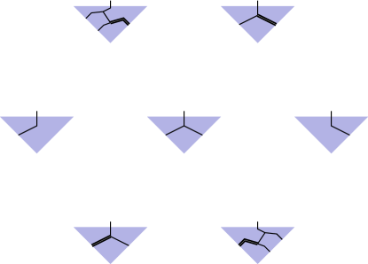
Figure 12: Triangular diagrams

.

Example 7.3.

We take the word aoA whose planar trivalent graph has a single trivalent vertex and so is invariant under rotation. We remove the initial a to get oA. Then we apply the lowering operators to get the following sequence of words

$$oA\rightarrow cA\rightarrow bA\rightarrow bB\rightarrow aB\rightarrow aC\rightarrow ao$$

Then we add the A at the end to get aoA. Alternatively, the word aoA is represented by

Then the sequence of words is represented by the sequence

$$\begin{array}[]{ccccc}&\includegraphics[width=36.135pt]{csp.29}&&\includegraphics[width=36.135pt]{csp.32}&\\ \includegraphics[width=36.135pt]{csp.27}&&\includegraphics[width=36.135pt]{csp.30}&&\includegraphics[width=36.135pt]{csp.33}\\ &\includegraphics[width=36.135pt]{csp.28}&&\includegraphics[width=36.135pt]{csp.31}&\end{array}$$

Example 7.4.

We start with the word abcAoA. We remove the initial a to get bcAoA. Then we apply the lowering operators to get the following vertices of a crystal

bcAoA
acAoA
abAoA
abAcA
abBcA
abBbA
abBbB

Then we add the A at the end to get abBbBA. This gives $abcAoA\mapsto abBbBA$.

Example 7.5.

We start with the word abBbBA. We remove the initial a to get bBbBA. Then we apply the lowering operators to get the following vertices of a crystal

bBbBA
aBbBA
aCbBA
aCaBA
aoaBA
aoaCA
aoaCB

Then we add the A at the end to get aoaCBA. This gives $abBbBA\mapsto aoaCBA$.

These examples support the following conjecture:

Conjecture 7.6.

The bijection in [56] between non-positive trivalent graphs with $r$ boundary points and isolated words in $\otimes^{r}B$ interwines rotation and promotion.

8 Energy statistic

A triple $(X,c,P)$ which exhibits the cyclic sieving phenomenon is more interesting from a combinatorial perspective if $P$ is the generating function of a statistic on $X$. That is, there is a function $\mathrm{st}\colon X\rightarrow\mathbb{N}$ such that $P=\sum_{x\in X}q^{\mathrm{st}(x)}$.

In this section we show that for some representations $P$ is a classically restricted one dimensional configuration sum. These polynomials are given by the fermionic formula and are the generating function for a statistic known as energy. The representations for which this holds are listed in section 8.2. This construction of examples of the cyclic sieving phenomenon still uses Proposition 6.4 but avoids Theorem 2.5.

The energy function is purely combinatorial but the representation theory background is the study of Kirillov-Reshetikhin modules. This is a large and difficult subject with its origins in the study of exactly solvable models in statistical mechanics.

8.1 Kirillov-Reshetikhin modules

Let $\mathfrak{g}$ be a semisimple Lie algebra. Then let $\widetilde{\mathfrak{g}}$ be the affine algebra of $\mathfrak{g}$ and $\widetilde{\mathfrak{g}}^{\prime}$ be its derived subalgebra. The affine algebra is infinite dimensional and the derived algebra has codimension one. The affine algebra is a Kac-Moody algebra and the derived algebra is defined by omitting the grading operator. The affine algebra has no non-trivial finite dimensional representations, whereas the derived algebra has an interesting category of finite dimensional representations. These both have quantised enveloping algebras. Our interest is in $U_{q}(\widetilde{\mathfrak{g}}^{\prime})$ and its category of finite dimensional representations.

The Yangian, $Y(\mathfrak{g})$, is a deformation of $U(\mathfrak{g}[t])$ associated with a Lie bialgebra structure on $\mathfrak{g}[t]$. The category of finite dimensional dimensional representations of $U_{q}(\widetilde{\mathfrak{g}}^{\prime})$ should be understood as a $q$-analogue of the category of finite dimensional dimensional representations of $Y(\mathfrak{g})$ even though it is not obvious that it is given by a deformation quantisation. One way this is made manifest is that a representation of $Y(\mathfrak{g})$ gives a rational solution to the Yang-Baxter equation (with spectral parameter) and a representation of $U_{q}(\widetilde{\mathfrak{g}}^{\prime})$ gives a trigonometric solution.

The most important, and best understood, representations of these quantum groups are the Kirillov-Reshetikhin modules (aka KR-modules) and their tensor products. There is a KR-module for each simple root $\alpha$ and each $s>0$. The associated module for the Yangian is denoted $W^{(\alpha,s)}$ and for the quantum affine algebra by $W_{q}^{(\alpha,s)}$. We refer the reader to the excellent survey, [4], for more information.

The property of the Kirillov-Reshetikhin modules we are interested in is that they have a crystal. In fact, these modules and their tensor products are the only known examples of finite dimensional representations of the quantum affine algebra which admit a crystal. The crystal of $W_{q}^{(\alpha,s)}$ is denoted $B^{(\alpha,s)}$. Two uniform constructions of these crystals are the alcove path model [30] and the level zero projection of Littelmann paths [32].

8.2 Classically irreducible modules

The pair $(\alpha,s)$ is classically irreducible if the classical restriction of $B^{(\alpha,s)}$ is connected. Equivalently, the restriction of $W_{q}^{(\alpha,s)}$ to $U_{q}(\mathfrak{g})$ is irreducible. In this case the restriction is the highest weight representation $V(s\omega_{\alpha})$.

First we list the fundamental representations $V(\omega_{\alpha})$ such that $W_{q}^{(\alpha,s)}$ is classically irreducible for all $s\geqslant 1$. For type $A$ these are all of the fundamental representations. For the remaining types the list is

Type $B$

the defining representation

Type $C$

the extreme fundamental representation whose dimension is a Catalan number

Type $D$

the defining representation and both half-spin representations

Type $E_{6}$

the dual pair of twenty seven dimensional representations

Type $E_{7}$

the fifty six dimensional representation

These are all perfect. These are also the nodes of the Dynkin diagram such that the corresponding coordinate of the null root, $\delta$, is $1$.

Next we list the fundamental representations $V(\omega_{\alpha})$ such that $W_{q}^{(\alpha,1)}$ is classically irreducible but $W_{q}^{(\alpha,2)}$ is classically reducible.

Type $B$

the spin representation

Type $C$

the defining representation

Type $G_{2}$

the seven dimensional representation

Type $F_{4}$

the twenty six dimensional representation

None of these are perfect.

Note that $E_{8}^{(1)}$ has no classically irreducible representation.

8.3 Current algebras

Let $\mathfrak{g}$ be a simple Lie algebra. The current algebra is the Lie algebra $\mathfrak{g}[t]=\mathfrak{g}\otimes\mathbb{C}[t]$. The Lie bracket is

$$[x\otimes f(t),y\otimes g(t)]=[x,y]\otimes f(t)g(t)$$

This has a grading where $t$ has degree 1 and this gives a grading on the universal enveloping algebra $U(\mathfrak{g}[t])$. Let $V$ be a finite dimensional representation of $U(\mathfrak{g}[t])$ together with a cyclic vector $v\in V$. This gives a filtration on $V$ by

$$V^{(i)}=\sum_{j\leqslant i}U(\mathfrak{g}[t])^{j}.v$$

The Yangian and the current algebra both have a family of automorphisms parametrised by $\mathbb{C}$. For the current algebra, the automorphisms $\tau_{c}$, for $c\in\mathbb{C}$, are given by

$$\tau_{c}\colon x\otimes f(t)\mapsto x\otimes f(t-c)$$

Then each representation, $V$, gives a family of representations by $V(c)=\tau_{c}^{*}V$.

Now let $V_{k}$ for $1\leqslant k\leqslant r$ be a sequence of representations each with a vector $v_{k}$ which generates the module. Then the tensor product $V_{1}(u_{1})\otimes\dotsb\otimes V_{r}(u_{r})$ has the cyclic vector $v_{1}\otimes\dotsb\otimes v_{r}$ provided the parameters are distinct. The fusion product, $V_{1}(u_{1})\ast\dotsb\ast V_{r}(u_{r})$, is the graded representation associated to the filtration on the tensor product representation with this choice of cyclic vector.

For any representation, $V$, of $\mathfrak{g}$ we have a family of representations of $\mathfrak{g}[t]$, $V(c)$ for $c\in\mathbb{C}$, where

$$(x\times f(t)).v=f(c)x.v$$

For any sequence ${[\bm{\alpha},\bm{s}]}$ and any distinct values of the parameters consider $W^{(\alpha_{1},s_{1})}(u_{1})\ast\dotsb\ast W^{(\alpha_{r},s_{r})}(u_{r})$ as a graded $\mathfrak{g}$-module. Then each isotypical component is a graded vector space. For a graded vector space $V=\oplus_{k}V^{[k]}$ the graded dimension is the polynomial

$$\sum_{k}\dim(V^{[k]})q^{k}$$

Then for all $\lambda\in P_{+}$ and all sequences ${[\bm{\alpha},\bm{s}]}$ define $C(\lambda,{[\bm{\alpha},\bm{s}]})$ to be the graded dimension of the isotypical component

$$\mathrm{Hom}_{\mathfrak{g}}(V(\mu),W^{(\alpha_{1},s_{1})}(u_{1})\ast\dotsb\ast W^{(\alpha_{r},s_{r})}(u_{r})$$

It is shown in [10] that for all $\lambda\in P_{+}$ and all sequences ${[\bm{\alpha},\bm{s}]}$ the polynomial $C(\lambda,{[\bm{\alpha},\bm{s}]})$ is independent of the choice of $u_{1},u_{2},\dots,u_{r}$.

Let $\zeta$ be a primitive $r$-th root of unity.

Proposition 8.1.

The long cycle acts by $\zeta^{k}$ on the component of degree $k$ of the fusion product $V(1)\ast V(\zeta)\ast\dotsb\ast V({\zeta^{r-1}})$.

The proof is from [11, §4.2].

Proof.

Let $\rho$ be the action of the long cycle given by

$$\rho(v_{1}\otimes\dotsb\otimes v_{r})=v_{2}\otimes\dotsb\otimes v_{r}\otimes v_{1}$$

Then $\rho$ commutes with the action of $\mathfrak{g}$ but not with the action of $\mathfrak{g}[t]$. Instead we have

$$x\otimes t^{k}\circ\rho=\zeta^{k}\rho\circ x\otimes t^{k}$$

∎

Then combining Proposition 6.4 and Proposition 8.1 gives the following example of the cyclic sieving phenomenon.

Theorem 8.2.

Let $W(\alpha,s)$ be classically irreducible. Put $X=(\otimes^{r}B(\omega_{\alpha}))_{\ast}$ with $c$ acting by promotion. Then $(X,c,P)$ exhibits the cyclic sieving phenomenon with $P=C(0,{[\bm{\alpha},\bm{s}]})$ where ${[\bm{\alpha},\bm{s}]}$ is the sequence with $(\alpha_{i},s_{i})=(\alpha,s)$ for $1\leqslant i\leqslant r$.

8.4 Energy function

Theorem 8.2 is unsatisfactory as it does not give any method for computing the polynomial. The polynomials $C(\lambda,{[\bm{\alpha},\bm{s}]})$ have several other interpretations. One of the interpretations is as the generating function for the energy function. As a polynomial this is given by the fermionic formula and this is an efficient formula for computing these polynomials.

There are two ways of constructing the energy function on highest weight words. Each involves some intricate combinatorics. One way is to define the energy function as a statistic on rigged configurations. It is a simple observation that the generating function is given by the fermionic formula. Indeed, this was the motivation for introducing rigged configurations. Then, in order to view the energy function as a statistic on highest weight words, a bijection between rigged configurations and highest weight words is required. The alternative is to define the energy function as a statistic on highest weight words directly. This approach uses the combinatorial $R$-matrices.

Example 8.3.

The polynomials in section 7 can be computed in sage using

sage: RC = RiggedConfigurations([’G’, 2, 1], [[1,1]]*4 )
sage: mg = RC.module_generators
sage: [ a.cc() for a in mg if a.weight() == 0 ]
[8, 6, 6, 4]

The result that the polynomials $C(\lambda,{[\bm{\alpha},\bm{s}]})$ are given by the fermionic formula has been proved not as an isolated result but in conjunction with several other conjectures. These include the conjectures set out in the remarkable paper [14]. We refer the interested reader to [24] which gives an overview.

References

- [1] François Bergeron, Gilbert Labelle and Pierre Leroux “Combinatorial species and tree-like structures” Translated from the 1994 French original by Margaret Readdy, With a foreword by Gian-Carlo Rota 67, Encyclopedia of Mathematics and its Applications Cambridge: Cambridge University Press, 1998, pp. xx+457
- [2] Wieb Bosma, John Cannon and Catherine Playoust “The Magma algebra system. I. The user language” Computational algebra and number theory (London, 1993) In J. Symbolic Comput. 24.3-4, 1997, pp. 235–265 DOI: 10.1006/jsco.1996.0125
- [3] Richard Brauer “On algebras which are connected with the semisimple continuous groups” In Ann. of Math. (2) 38.4, 1937, pp. 857–872 DOI: 10.2307/1968843
- [4] Vyjayanthi Chari and David Hernandez “Beyond Kirillov-Reshetikhin modules” In Quantum affine algebras, extended affine Lie algebras, and their applications 506, Contemp. Math. Amer. Math. Soc., Providence, RI, 2010, pp. 49–81 DOI: 10.1090/conm/506/09935
- [5] Predrag Cvitanović “Group theory” Birdtracks, Lie’s, and exceptional groups Princeton University Press, Princeton, NJ, 2008, pp. xiv+273 DOI: 10.1515/9781400837670
- [6] Jacques Désarménien “Fonctions symétriques associées à des suites classiques de nombres” In Ann. Sci. École Norm. Sup. (4) 16.2, 1983, pp. 271–304 URL: http://www.numdam.org/item?id=ASENS_1983_4_16_2_271_0
- [7] Satyan L. Devadoss “Tessellations of moduli spaces and the mosaic operad” In Homotopy invariant algebraic structures (Baltimore, MD, 1998) 239, Contemp. Math. Amer. Math. Soc., Providence, RI, 1999, pp. 91–114 DOI: 10.1090/conm/239/03599
- [8] V. G. Drinfel$^$d “Hopf algebras and the quantum Yang-Baxter equation” In Dokl. Akad. Nauk SSSR 283.5, 1985, pp. 1060–1064
- [9] V. G. Drinfel$^$d “Quantum groups” In Proceedings of the International Congress of Mathematicians, Vol. 1, 2 (Berkeley, Calif., 1986) Amer. Math. Soc., Providence, RI, 1987, pp. 798–820
- [10] B. Feigin and S. Loktev “On generalized Kostka polynomials and the quantum Verlinde rule” In Differential topology, infinite-dimensional Lie algebras, and applications 194, Amer. Math. Soc. Transl. Ser. 2 Amer. Math. Soc., Providence, RI, 1999, pp. 61–79 URL: http://arxiv.org/abs/math/9812093
- [11] Bruce Fontaine and Joel Kamnitzer “Cyclic sieving, rotation, and geometric representation theory” In Selecta Math. (N.S.) 20.2, 2014, pp. 609–625 DOI: 10.1007/s00029-013-0144-4
- [12] Igor B. Frenkel and Mikhail G. Khovanov “Canonical bases in tensor products and graphical calculus for ” In Duke Math. J. 87.3, 1997, pp. 409–480 DOI: 10.1215/S0012-7094-97-08715-9
- [13] Adriano M. Garsia “Combinatorics of the free Lie algebra and the symmetric group” In Analysis, et cetera Academic Press, Boston, MA, 1990, pp. 309–382
- [14] Goro Hatayama et al. “Paths, crystals and fermionic formulae” In MathPhys odyssey, 2001 23, Prog. Math. Phys. Birkhäuser Boston, Boston, MA, 2002, pp. 205–272 URL: https://arxiv.org/abs/math/0102113
- [15] André Henriques and Joel Kamnitzer “Crystals and coboundary categories” In Duke Math. J. 132.2, 2006, pp. 191–216 DOI: 10.1215/S0012-7094-06-13221-0
- [16] Jin Hong and Seok-Jin Kang “Introduction to quantum groups and crystal bases” 42, Graduate Studies in Mathematics Providence, RI: American Mathematical Society, 2002, pp. xviii+307
- [17] Jens Carsten Jantzen “Lectures on quantum groups” 6, Graduate Studies in Mathematics Providence, RI: American Mathematical Society, 1996, pp. viii+266
- [18] André Joyal and Ross Street “The geometry of tensor calculus. I” In Adv. Math. 88.1, 1991, pp. 55–112 DOI: 10.1016/0001-8708(91)90003-P
- [19] A. Jucys, J. Levinsonas and V. Vanagas “Matematicheskii apparat teorii momenta kolichestva dvizheniya” Akad. Nauk Litovsk. SSR, Inst. Fiz. i Mat. Publ. No. 3. Gosudarstv. Izdat. Politič. i Nauč. Lit. Litovsk. SSR, Vilna, 1960, pp. 243
- [20] Joel Kamnitzer “Mirković-Vilonen cycles and polytopes” In Ann. of Math. (2) 171.1, 2010, pp. 245–294 DOI: 10.4007/annals.2010.171.245
- [21] Joel Kamnitzer and Peter Tingley “The crystal commutor and Drinfeld’s unitarized -matrix” In J. Algebraic Combin. 29.3, 2009, pp. 315–335 DOI: 10.1007/s10801-008-0137-0
- [22] Masaharu Kaneda “Based modules and good filtrations in algebraic groups” In Hiroshima Math. J. 28.2, 1998, pp. 337–344 URL: https://projecteuclid.org/euclid.hmj/1206126765
- [23] Masaki Kashiwara “Crystalizing the -analogue of universal enveloping algebras” In Comm. Math. Phys. 133.2, 1990, pp. 249–260 URL: https://projecteuclid.org/euclid.cmp/1104201397
- [24] Rinat Kedem “A pentagon of identities, graded tensor products, and the Kirillov-Reshetikhin conjecture” In New trends in quantum integrable systems World Sci. Publ., Hackensack, NJ, 2011, pp. 173–193 DOI: 10.1142/9789814324373˙0010
- [25] G. M. Kelly and M. L. Laplaza “Coherence for compact closed categories” In J. Pure Appl. Algebra 19, 1980, pp. 193–213 DOI: 10.1016/0022-4049(80)90101-2
- [26] Daan Krammer “Generalisations of the Tits representation” In Electron. J. Combin. 15.1, 2008, pp. Research Paper 134, 28 URL: http://arxiv.org/abs/0708.1273
- [27] Witold Kraśkiewicz and Jerzy Weyman “Algebra of coinvariants and the action of a Coxeter element” In Bayreuth. Math. Schr., 2001, pp. 265–284
- [28] Greg Kuperberg “Spiders for rank Lie algebras” In Comm. Math. Phys. 180.1, 1996, pp. 109–151 URL: arXiv.org:q-alg/9712003
- [29] M.A.A. Leeuwen, A.M. Cohen and B. Lisser “LiE, A package for Lie Group Computations”, 1992 URL: http://wwwmathlabo.univ-poitiers.fr/~maavl/LiE/
- [30] Cristian Lenart et al. “A uniform model for Kirillov-Reshetikhin crystals” In 25th International Conference on Formal Power Series and Algebraic Combinatorics (FPSAC 2013), Discrete Math. Theor. Comput. Sci. Proc., AS Assoc. Discrete Math. Theor. Comput. Sci., Nancy, 2013, pp. 25–36
- [31] Peter Littelmann “Crystal graphs and Young tableaux” In J. Algebra 175.1, 1995, pp. 65–87 DOI: 10.1006/jabr.1995.1175
- [32] Peter Littelmann “Paths and root operators in representation theory” In Ann. of Math. (2) 142.3, 1995, pp. 499–525 DOI: 10.2307/2118553
- [33] G. Lusztig “Canonical bases arising from quantized enveloping algebras” In J. Amer. Math. Soc. 3.2, 1990, pp. 447–498 DOI: 10.2307/1990961
- [34] G. Lusztig “Canonical bases arising from quantized enveloping algebras. II” Common trends in mathematics and quantum field theories (Kyoto, 1990) In Progr. Theoret. Phys. Suppl., 1990, pp. 175–201 (1991) DOI: 10.1143/PTPS.102.175
- [35] G. Lusztig “Quantum deformations of certain simple modules over enveloping algebras” In Adv. in Math. 70.2, 1988, pp. 237–249 DOI: 10.1016/0001-8708(88)90056-4
- [36] George Lusztig “Introduction to quantum groups” 110, Progress in Mathematics Boston, MA: Birkhäuser Boston Inc., 1993, pp. xii+341
- [37] George Lusztig “The canonical basis of the quantum adjoint representation”, 2016 URL: http://arxiv.org/abs/1602.07276
- [38] Saunders Mac Lane “Natural associativity and commutativity” In Rice Univ. Studies 49.4, 1963, pp. 28–46 URL: https://scholarship.rice.edu/handle/1911/62865
- [39] I. G. Macdonald “Symmetric functions and Hall polynomials” With contributions by A. Zelevinsky, Oxford Science Publications, Oxford Mathematical Monographs The Clarendon Press, Oxford University Press, New York, 1995, pp. x+475
- [40] I. Mirković and K. Vilonen “Geometric Langlands duality and representations of algebraic groups over commutative rings” In Ann. of Math. (2) 166.1, 2007, pp. 95–143 DOI: 10.4007/annals.2007.166.95
- [41] Roger Penrose and Wolfgang Rindler “Spinors and space-time. Vol. 1” Two-spinor calculus and relativistic fields, Cambridge Monographs on Mathematical Physics Cambridge: Cambridge University Press, 1984, pp. x+458
- [42] T. Kyle Petersen, Pavlo Pylyavskyy and Brendon Rhoades “Promotion and cyclic sieving via webs” In J. Algebraic Combin. 30.1, 2009, pp. 19–41 DOI: 10.1007/s10801-008-0150-3
- [43] J. Howard Redfield “The Theory of Group-Reduced Distributions” In Amer. J. Math. 49.3, 1927, pp. 433–455 DOI: 10.2307/2370675
- [44] V. Reiner, D. Stanton and D. White “The cyclic sieving phenomenon” In J. Combin. Theory Ser. A 108.1, 2004, pp. 17–50 URL: www.math.umn.edu/~reiner/Papers/cycsieve.ps
- [45] Victor Reiner, Dennis Stanton and Dennis White “What is …cyclic sieving?” In Notices Amer. Math. Soc. 61.2, 2014, pp. 169–171 DOI: 10.1090/noti1084
- [46] Christophe Reutenauer “Free Lie algebras” Oxford Science Publications 7, London Mathematical Society Monographs. New Series The Clarendon Press, Oxford University Press, New York, 1993, pp. xviii+269
- [47] Brendon Rhoades “Cyclic sieving, promotion, and representation theory” In J. Combin. Theory Ser. A 117.1, 2010, pp. 38–76 DOI: 10.1016/j.jcta.2009.03.017
- [48] Claus Michael Ringel “Hall algebras and quantum groups” In Invent. Math. 101.3, 1990, pp. 583–591 DOI: 10.1007/BF01231516
- [49] Martin Rubey and Bruce W. Westbury “A combinatorial approach to classical representation theory”, 2014 URL: http://arxiv.org/abs/1408.3592
- [50] Bruce E. Sagan “The cyclic sieving phenomenon: a survey” In Surveys in combinatorics 2011 392, London Math. Soc. Lecture Note Ser. Cambridge Univ. Press, Cambridge, 2011, pp. 183–233 URL: http://arxiv.org/abs/1008.0790
- [51] Alistair Savage “Braided and coboundary monoidal categories” In Algebras, representations and applications 483, Contemp. Math. Amer. Math. Soc., Providence, RI, 2009, pp. 229–251 DOI: 10.1090/conm/483/09448
- [52] Mei Chee Shum “Tortile tensor categories” In J. Pure Appl. Algebra 93.1, 1994, pp. 57–110 DOI: 10.1016/0022-4049(92)00039-T
- [53] N. J. A. Sloane “The On-Line Encyclopedia of Integer Sequences”, 2008 URL: www.research.att.com/~njas/sequences/.
- [54] Richard P. Stanley “Enumerative combinatorics. Vol. 2” With a foreword by Gian-Carlo Rota and appendix 1 by Sergey Fomin 62, Cambridge Studies in Advanced Mathematics Cambridge: Cambridge University Press, 1999, pp. xii+581
- [55] W.. Stein “Sage Mathematics Software (Version 7.1)”, 2016 The Sage Development Team URL: http://www.sagemath.org
- [56] Bruce W. Westbury “Enumeration of non-positive planar trivalent graphs” In J. Algebraic Combin. 25.4, 2007, pp. 357–373 DOI: 10.1007/s10801-006-0041-4