Dr. Jose Wagner Furtado Valle, Professor d’Investigació del Consejo Superior de Investigaciones Científicas, adscrit a l’Institut de Física Corpuscular - Departament de Física Teòrica, Universitat de València, i

Dr. Ricard Tomàs Bayo, investigador postdoctoral al II. Institut für Theoretische Physik, Universität Hamburg,

CERTIFIQUEM:

Que la present memòria “Supernoves com a laboratoris de propietats de neutrins” ha sigut realitzada sota la nostra direcció al Departament de Física Teòrica de la Universitat de València, per N’Andreu Esteban Pretel i constitueix la seua Tesi per tal d’optar al grau de Doctor en Física.

I perquè així conste, en compliment de la legislació vigent, presentem davant del Departamet de Física Teòrica de la Universitat de València la referida Tesi.

Prefaci

La física de neutrins ha experimentat un avanç espectacular en els darrers deu anys. En juny de 1998, la col$\cdot$laboració Super-Kamiokande [1] donà el primer pas important en aquest sentit en observar una forta evidència de conversió de sabor en els neutrins atmosfèrics, produïts en la col$\cdot$lisió de raigs còsmics amb l’atmosfera. No obstant, aquest resultat no fou una sorpresa completament, ja que durant les dues dècades anteriors s’havia obtingut indicacions en favor d’aquesta hipòtesi. En experiments amb neutrins solars i dades prèvies de neutrins atmosfèrics s’observava respectivament un dèficit de neutrins electrònics i neutrins muònics en relació als predits pels models teòrics. Discrepàncies conegudes com el problema dels neutrins solars i l’anomalia dels neutrins atmosfèrics. En 2002 es va confirmar l’oscil$\cdot$lació de neutrins, amb un esquema de massa i mescla, com el mecanisme correcte per a explicar el problema del dèficit de neutrins solars. Per demostrar-ho, van ser prou les primeres dades obtingudes per la col$\cdot$laboració KamLand [2], experiment terrestre amb neutrins generats en reactors nuclears. En eixe mateix sentit, i també en 2002, va ser resolta l’anomalia dels neutrins atmosfèrics fent ús de les dades de neutrins d’accelerador obtingudes en l’experiment K2K [3]. Més tard MINOS [4] no només confirmaria aquest resultat, sinó que augmentaria, i continua fent-ho, la precisió en la determinació dels corresponents paràmetres d’oscil$\cdot$lació.

La prova experimental de l’oscil$\cdot$lació de neutrins demostrava doncs que aquests tenen massa i, essent partícules sense massa dins del Model Estàndard (SM) de les interaccions electrofebles, això suposava alhora la primera evidència robusta de física més enllà del SM. Amb els experiments de neutrins a les portes de l’era de la precisió [5], la determinació de les propietats dels neutrins i el seu impacte teòric és un dels principals objectius per als físics d’astropartícules i d’altes energies [6]. Així doncs els principals esforços se centren actualment, per una banda en la identificació de la seua naturalesa, Dirac o Majorana, i per una altra banda en la determinació precisa dels paràmetres d’oscil$\cdot$lació i, de forma complementària, en la verificació de possibles efectes subdominants no oscil$\cdot$latoris, tals com la conversió d’espín i sabor [7, 8] o possibles interaccions no estàndard (NSI d’ací endavant) dels neutrins [9]. La determinació d’aquests obriria una finestra única per a explorar física més enllà del SM.

La tesi que ací es presenta pretén ser una anàlisi de diversos aspectes de fenomenologia de neutrins en dos escenaris diferents. D’un costat, es tracta l’estudi de les NSI en experiments terrestres d’accelerador i reactor. D’altre costat es discuteix la propagació de neutrins de supernova (SN), tenint en compte els nous descobriments que mostren la importància que el propi fons de neutrins té en l’evolució d’aquests. Aquest efecte, menyspreat durant molt de temps, pot ser de vital importància a l’hora d’entendre el senyal que una possible explosió de SN a la nostra galàxia donaria als detectors de neutrins. L’anàlisi dels neutrins de SN es presenta tant en absència com en presència de NSI.

La presència de NSI pot afectar dràsticament a la propagació dels neutrins en matèria, així doncs és important discutir les implicacions d’incloure aquestes interaccions en les anàlisis dels experiments terrestres previstos de neutrins d’accelerador i reactor. D’aquesta manera s’ha considerat l’efecte que les NSI poden tindre en els experiments MINOS, OPERA i Double Chooz [10], i per tant els límits que d’aquests es pot obtenir. La motivació del treball és doble, d’un costat tots tres experiments estaran funcionant durant els propers anys, per tant és una informació de la que disposarem en un futur pròxim. D’altre costat, OPERA mesurarà per primera vegada l’oscil$\cdot$lació $\nu_{\mu}\to\nu_{\tau}$ detectant directament els $\nu_{\tau}$ i té, a més a més, una relació distancia-energia ($L/E$) molt diferent a la de MINOS, dues característiques que és sabut que ajuden en l’estudi de les NSI. Els límits que d’aquest estudi i d’altres previs s’extrauen seran utilitzats en l’anàlisi de l’efecte de les NSI en la propagació de neutrins de SN.

L’estudi de neutrins de SN ve motivat principalment per dues raons. En primer lloc, si una explosió de SN es donés a la nostra galàxia, el nombre d’esdeveniments que s’observarien en els experiments presents i futurs seria enorme, de l’ordre de $\mathcal{O}(10^{4}$–$10^{5})$. En segon lloc, les condicions extremes que els neutrins travessarien des que són creats al nucli de la SN fins ser detectats a la terra, tindria un efecte dràstic en la seua propagació. En aquest estudi farem especial èmfasi en l’efecte que els propis neutrins tenen en la seua evolució. Al dens flux de neutrins que emergeix del nucli d’una SN la refracció neutrí-neutrí causa un fenomen de conversió de sabor no lineal que és completament diferent a qualsevol efecte induït per la matèria ordinària [11, 12, 13, 14, 15, 16, 17, 18, 19, 20]. El principal efecte és un mode col$\cdot$lectiu de transformació de parells de la forma $\nu_{e}\bar{\nu}_{e}\to\nu_{x}\bar{\nu}_{x}$, on $\nu_{x}$ correspon a una superposició de $\nu_{\mu}$ i $\nu_{\tau}$. Per tindre aquest procés es necessari una gran densitat de neutrins i un excés de parells d’algun sabor. Ambdues condicions estan presents als models típics de SN.

D’un altre costat, com ja s’ha comentat, es presentarà l’efecte que pot tindre l’existència de NSI en l’evolució de neutrins de SN, estudi que es presentarà tant en absència [21], com en presència [22] d’autointeracció dels neutrins. Una explosió de SN és un bon escenari per a fer aquesta anàlisi, ja que els efectes de NSI xicotetes poden veure’s amplificats degut a les condicions extremes de densitat de matèria que troben els neutrins en la seua propagació.

Així doncs, la present tesi està organitzada de la següent forma. Al Capítol 1 resumim els coneixements actuals sobre la física de les SNe que esclaten per col$\cdot$lapse gravitatori del nucli. Al Capítol 2 discutim el fenomen d’oscil$\cdot$lació de neutrins tant per a dos com per a tres sabors, en buit i en matèria, i sempre en absència d’un fons de neutrins. Al final d’aquest capítol apliquem el formalisme descrit anteriorment per a estudiar l’evolució de neutrins en l’embolcall d’una SN. Al Capítol 3 analitzem com la inclusió de les NSI afecta a l’evolució dels neutrins i recordem els límits actuals sobre els paràmetres que les caracteritzen. A més a més, estudiem el que es pot aprendre d’aquestes amb els resultats dels experiments MINOS, OPERA i Double Chooz. Els Capítols 4 i 5 els dediquem a l’estudi dels efectes de l’autointeracció dels propis neutrins en una SN. Al primer d’aquests capítols, després de resumir el coneixement que del fenomen de transformació col$\cdot$lectiva de neutrins es té actualment, centrem la discussió en un escenari de dos sabors i tractem la qüestió dels efectes multiangulars en aquest fenomen. El Capítol 5 el dediquem a l’anàlisi de possibles efectes característics de tres neutrins. Al Capítol 6 estudiem les conseqüències de les NSI dels neutrins en la seua evolució en una SN. Per tal de distingir els efectes derivats de les NSI d’aquells que vénen de l’autointeracció dels neutrins, comencem menyspreants aquests últims. A la segona part del capítol incloem ja tots els ingredients i discutim el seu efecte conjunt. Per últim, al Capítol 7 fem un breu resum de tot allò analitzat en aquesta tesi doctoral remarcant el punts que considerem més importants del treball.

Tots els resultats originals discutits en aquesta tesi doctoral han sigut publicats en les Refs. [10, 17, 18, 20, 21, 22]:

• A. Esteban-Pretel, R. Tomàs and J. W. F. Valle, “Probing non-standard neutrino interactions with supernova neutrinos,” Phys. Rev. D 76 (2007) 053001 [arXiv:0704.0032 [hep-ph]].

• A. Esteban-Pretel, S. Pastor, R. Tomàs, G. G. Raffelt and G. Sigl, “Decoherence in supernova neutrino transformations suppressed by deleptonization,” Phys. Rev. D 76 (2007) 125018 [arXiv:0706.2498 [astro-ph]].

• A. Esteban-Pretel, S. Pastor, R. Tomàs, G. G. Raffelt and G. Sigl, “Mu-tau neutrino refraction and collective three-flavor transformations in supernovae,” Phys. Rev. D 77 (2008) 065024 [arXiv:0712.1137 [astro-ph]].

• A. Esteban-Pretel, J. W. F. Valle and P. Huber, “Can OPERA help in constraining neutrino non-standard interactions?,” Phys. Lett. B 668 (2008) 197 [arXiv:0803.1790 [hep-ph]].

• A. Esteban-Pretel, A. Mirizzi, S. Pastor, R. Tomàs, G. G. Raffelt, P. D. Serpico and G. Sigl, “Role of dense matter in collective supernova neutrino transformations,” Phys. Rev. D 78 (2008) 085012 [arXiv:0807.0659 [astro-ph]].

• A. Esteban-Pretel, R. Tomàs and J. W. F. Valle, “Interplay between collective effects and non-standard neutrino interactions of supernova neutrinos,” arXiv:0909.2196 [hep-ph].

Preface

Neutrino physics has experienced a spectacular breakthrough in the last ten years. In June 1998, the Super-Kamiokande Collaboration [1] gave the first important step in this direction when they observed a strong evidence of flavor conversion for atmospheric neutrinos, those produced from the collision of cosmic rays with the atmosphere. However, this result was not a complete surprise. For two decades indications favoring this hypothesis had been obtained. A deficit of electron and muon neutrinos, compared to the prediction of theoretical models, was observed in solar neutrino experiments and previous atmospheric neutrino data, respectively. These discrepancies are known as the solar neutrino problem and the atmospheric neutrino anomaly. In 2002, flavor neutrino oscillation, within a scheme of mass and mixing, was confirmed as the correct mechanism to explain the solar neutrino deficit problem. The first data obtained by the KamLAND [2] collaboration, a terrestrial experiment detecting reactor neutrinos, were enough to demonstrate this oscillation scenario. In the same direction, and also in 2002, the atmospheric neutrino anomaly was explained using the accelerator neutrino data obtained in the K2K [3] experiment. Later on, MINOS [4] would not only confirm this result but would also increase, and continues to do so, the precision in the determination of the corresponding oscillation parameters.

The experimental evidence of neutrino oscillations proved that they have mass. Therefore, neutrinos being massless within the electro-weak Standard Model (SM), it also represented the first robust evidence of physics beyond the SM. With neutrino experiments at the threshold of the precision era [5], the determination of neutrino properties and their theoretical impact is one of the main goals for astroparticle and high energy physicists [6]. Most of the effort is nowadays focused on the precise determination of the oscillation parameters and, in a complementary way, on the verification of possible sub-leading non-oscillation effects, such as spin and flavor conversions [7, 8] or possible non-standard neutrino interactions (NSI from now on) [9]. Their determination would open a unique window to explore physics beyond the SM.

The present thesis aims to be an analysis of various aspects of neutrino phenomenology in two different scenarios. On the one hand, we address the study of neutrino NSI in accelerator and reactor terrestrial experiments. On the other hand, we discuss the propagation of supernova (SN) neutrinos, taking into account the recent developments showing the importance that neutrino background may have in their evolution. This effect, neglected for a long time, may be of capital importance when trying to understand the neutrino signal from a future galactic SN. Our SN neutrino analysis is presented both in absence and presence of NSI.

The presence of NSI may drastically affect the propagation of neutrinos through matter. Thus, it is important to discuss the implications of including these new interactions in the future planned neutrino terrestrial experiments. In this sense, we have considered the effects that NSI may induce in MINOS, OPERA and Double Chooz experiments [10], and the bounds that can be obtained from them. The motivation of the work is twofold, on the one hand all three experiments will be taking data during the next years, providing valuable information in the near future. On the other hand, OPERA will measure for the first time the oscillation channel $\nu_{\mu}\to\nu_{\tau}$, detecting directly the $\nu_{\tau}$. Moreover, it has a very different distance-energy ratio ($L/E$) than MINOS. Both factors are expected to help in disentangling NSI from pure oscillations. The bounds obtained in this study and the previous ones will be used in the analysis of NSI effects in the propagation of SN neutrinos.

The study of SN neutrinos is motivated mainly by two reasons. First, if a future SN explosion takes place in our galaxy, an enormous number of neutrino events are expected in the present and future planned detectors, $\mathcal{O}(10^{4}$–$10^{5})$. Second, the extreme conditions under which neutrinos travel since they are created in the SN core until they are detected at the Earth, would have a dramatic effect in their propagation. In our study we pay special attention to the effect of the neutrino background itself. In the dense neutrino flux emerging from a SN core, neutrino-neutrino refraction causes non-linear flavor conversion phenomena that are unlike anything produced by ordinary matter [11, 12, 13, 14, 15, 16, 17, 18, 19, 20]. The crucial phenomenon is a collective mode of pair transformations of the form $\nu_{e}\bar{\nu}_{e}\to\nu_{x}\bar{\nu}_{x}$ where $x$ represents a suitable superposition of $\nu_{\mu}$ and $\nu_{\tau}$. Collective pair transformations require a large neutrino density and a pair excess of a given flavor. Both conditions are present in typical SN models.

On the other hand, as it has already been commented, we will discuss the effect that the existence of NSI would have in the evolution of SN neutrinos. This study will be done both in absence [21], and presence [22] of neutrino-neutrino interactions. A SN explosion is an attractive scenario to study NSI, since the effect of small NSI can be amplified due to the extreme conditions found in the SNe.

The present thesis is therefore organized as follows. In Chapter 1 we review the current knowledge on core collapse SN physics. In Chapter 2 we discuss the neutrino oscillation phenomenon for two and three flavors, in vacuum and matter, but always in the absence of a neutrino background. At the end of this chapter we apply the formalism previously described to study the evolution of neutrinos through the SN envelope. In Chapter 3 we analyze how the inclusion of NSI affects the evolution of neutrinos and review the current bounds on the parameters that characterize them. Furthermore, we study what we can learn about NSI from the results of MINOS, OPERA and Double Chooz experiments. Chapters 4 and 5 are devoted to the study of neutrino-neutrino interactions in the SN context. In the first one, after reviewing the current knowledge on the collective neutrino transformation phenomenon, we center the discussion in the two flavor scenario and address the question of multi-angle effects in this phenomenon. In Chapter 5 we analyze the possible three flavor characteristic effects. In Chapter 6 we study the consequences that NSI would have in neutrino evolution through the SN envelope. In order to separate the effects of NSI from those of neutrino-neutrino interaction, we start by neglecting the latter. In the second part of the chapter we include all the ingredients, and discuss the interplay among them. Finally, in chapter 7 we briefly summarize the topics discussed in the present Ph.D. thesis emphasizing the points that we consider of most interest.

All the original results presented in this Ph.D. thesis have been published in Refs. [10, 17, 18, 20, 21, 22]:

• A. Esteban-Pretel, R. Tomàs and J. W. F. Valle, “Probing non-standard neutrino interactions with supernova neutrinos,” Phys. Rev. D 76 (2007) 053001 [arXiv:0704.0032 [hep-ph]].

• A. Esteban-Pretel, S. Pastor, R. Tomàs, G. G. Raffelt and G. Sigl, “Decoherence in supernova neutrino transformations suppressed by deleptonization,” Phys. Rev. D 76 (2007) 125018 [arXiv:0706.2498 [astro-ph]].

• A. Esteban-Pretel, S. Pastor, R. Tomàs, G. G. Raffelt and G. Sigl, “Mu-tau neutrino refraction and collective three-flavor transformations in supernovae,” Phys. Rev. D 77 (2008) 065024 [arXiv:0712.1137 [astro-ph]].

• A. Esteban-Pretel, J. W. F. Valle and P. Huber, “Can OPERA help in constraining neutrino non-standard interactions?,” Phys. Lett. B 668 (2008) 197 [arXiv:0803.1790 [hep-ph]].

• A. Esteban-Pretel, A. Mirizzi, S. Pastor, R. Tomàs, G. G. Raffelt, P. D. Serpico and G. Sigl, “Role of dense matter in collective supernova neutrino transformations,” Phys. Rev. D 78 (2008) 085012 [arXiv:0807.0659 [astro-ph]].

• A. Esteban-Pretel, R. Tomàs and J. W. F. Valle, “Interplay between collective effects and non-standard neutrino interactions of supernova neutrinos,” arXiv:0909.2196 [hep-ph].

Chapter 1 Core Collapse Supernovae

One of the most spectacular cosmic events is a core collapse supernova (SN) explosion. It means the death of a massive star and gives birth to the most exotic states of matter known, neutron stars and black holes. SN explosions determine also the evolution of galaxies, since most of the heavy elements in nature, with mass number $A>70$, are thought to be created through the s- and r- (slow and rapid) processes. It has long been thought that the latter take place in this kind of events. Elements that will afterwards serve as raw material in the creation of new stars and planets.

Such an event involves as much instantaneous power as all the rest of the luminous visible Universe combined, it releases about $10^{52}$ erg s^-1 ($\sim 10^{45}$ J s^-1) during some tens of seconds. Around 99% of this energy is emitted as neutrinos. They are, therefore, expected to play a crucial role in the SN evolution.

There exist, though, different types of SNe, and not all of them are the consequence of the collapse of a massive star core.

1.1 Supernova types

The work of SN classification started with Minkowski [23] (1941) who divided them in two types, whether they did (type II) or did not (type I) show hydrogen lines in their spectra. Nevertheless, a detailed classification of SNe according to observational criteria needs, besides the identification of the characteristics in the spectrum, an analysis of the line profile, luminosities and spectral evolution. In Fig. 1.1 we show this classification schematically.

Another criterion used in the classification of SNe is according to the explosion mechanism, under which we can distinguish two big groups: thermonuclear and core collapse explosions.

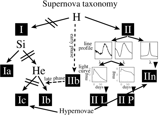
Figure 1.1: SN classification according to observational criteria [24].

1.1.1 SNIa: Thermonuclear explosion

SNIa are quite homogeneous events with similar luminosity and spectral evolutions. Indeed until the 1990s it was commonly accepted that all SNIa explosions were identical, and that the observed differences came from observational errors. Thanks to this homogeneity this kind of SNe are used as standard candles in determining distances to far galaxies. Type Ia SNe also provide a strong evidence for an accelerating Universe, and are the best single tool for directly measuring the density of dark energy.

From an observational point of view, their spectrum is characterized by the absence of hydrogen lines and the presence of silicon lines, see Fig. 1.1. The emission of elements like oxygen is not very important, which means that the progenitor star was not very massive. They have been observed in elliptical and spiral galaxies formed by old stars.

According to these observational features, the standard scenario for the SNIa explosion consists of a binary system where one of the stars is a white dwarf which accretes matter from the secondary star. The increment in mass leads to an increment in temperature for the central region of the star, until the threshold temperature of the carbon burning is reached. The high degeneracy of the stellar material turns the combustion regime unstable and triggers the thermonuclear explosion. After the explosion the progenitor star is completely destroyed, resulting in an expanding nebula without a central compact object.

The total energy released in type Ia SNe is approximately $3\times 10^{51}$ erg. Neutrinos carry just the 1% of this energy, and thus do not seem to play an important role in thermonuclear SNe. Since neutrinos are the main subject of this thesis, we will not further discuss this type of SN.

1.1.2 SNIb, SNIc, SNII: Core collapse explosion

The second group of SNe is much more heterogeneous. On the one hand, SNIb and SNIc, just as SNIa, do not have hydrogen lines in their spectra, but contrary to these, SNIb and SNIc also show an absence of silicon lines. Finally, SNIb present helium lines, while SNIc do not.

On the other hand we have type II SNe which contain hydrogen in the spectrum. These are also subclassified: SNII-P, in which after a maximum the luminosity curve remains fairly constant for 2–3 months, forming a plateau (e.g. SN 1987A), see Fig. 1.1; SNII-L, in which the luminosity falls rather linearly with time. Nevertheless, there is no clear separation between these two SN types and lots of intermediate cases exist. A third subtype of SNII is known as IIn, where the “n” stands for narrow-line, since their spectra show narrow components on top of the broader emissions. They are very bright and show a slow evolution. Some SNe seem to change along their evolution from a SNII, in the early phases, to a SNIb in the nebular phase, and are therefore classified as SNIIb. Finally, one very interesting development in the field of SNe has been the discovery of a very energetic type of them in the late 1990s, known as Hypernovae. The kinetic energy of such an event exceeds $10^{52}$ erg, which is 10 times larger than that of a usual SN explosion. These high energetic SNe have been observed as type Ic and IIn, and some hints exist that they might be related to $\gamma$-ray bursts [25].

This kind of explosions have been observed mainly in regions populated by young stars and presenting high stellar formation activity, like the arms of spiral galaxies. This is due to the fact that the evolution of this type of SN is much faster than the SNIa type. They are also less luminous than these and present a heterogeneous behavior on every aspect. More specifically the luminosity curves are different for each case, depending on the structure of the progenitor star. They are therefore not useful as standard candles.

The differences in the SN spectra are due to the loss of different envelope layers at some point of the evolution: SNIb ejects the hydrogen layer while SNIc also loses the helium layer. In spite of these spectral differences, SNIb, SNIc and SNII are all the result of the same explosion mechanism, related to the death of massive stars ($M\gtrsim 8M_{\odot}$). At the end of their life, massive stars accumulate iron in their center after several nuclear burning stages. When the iron core reaches a certain mass it becomes unstable and the collapse starts. According to the so called delayed explosion mechanism, the collapse is inverted into an explosion and a shock wave traverses the star, expelling the material found in its way. This explosion is accompanied with the formation of a neutron star or a black hole.

The total energy released in this kind of explosion is of the order of $10^{53}$ erg, from which only the $1$% is released as kinetic energy of the expelled material and approximately $0.01$% as light. The rest of the energy is emitted in the form of neutrinos, which will, therefore, be very important in the core collapse SN explosions, and may play a determinant role in the effective realization of the process.

The detection of neutrinos coming from such an event would be crucial for different reasons:

• Neutrinos, contrary to photons, emerge from the deepest regions of the star, since they are much more weakly interacting particles than photons. Neutrino detection would therefore be the only way, apart from gravitational waves, to obtain information of the inner layers of the star, highly important for the understanding of the explosion mechanism.

• While neutrinos escape the star seconds after the collapse, photons remain trapped and are only emitted from the envelope with a delay of several hours with respect to them. Therefore, neutrinos are the first signal expected from the explosion and could serve as an early warning system for galactic SNe.

• It can occur that the SN is optically obscured, or that the stellar collapse does not produce an explosion and creates a black hole. In such cases, the detection of neutrinos would be very important if not the only observable effect of the SN.

1.2 Core collapse supernova dynamics

The main topic of the present thesis is SNe as neutrino sources, thus we will study the type of SN where neutrinos play an important role, namely core collapse SNe (SNIb, SNIc and SNII). In order to understand the physical processes involved in the SN, it is useful to distinguish four stages in the phenomenon:

• The life of the progenitor star

• Stellar core collapse

• Deleptonization and cooling

• Supernova explosion

1.2.1 The life of the progenitor star

During its life a star must keep an equilibrium between two possible fatal effects working in opposite directions. On the one hand the gravitational force tends to collapse the star, on the other hand the thermal pressure tends to expand it. In order to maintain this equilibrium the star will undergo a series of nuclear burning stages.

Initially the hydrogen in the star will be transformed into helium through nuclear fusion reactions. When there is no more hydrogen in the center of the star this process can no longer compensate the gravitational force. As the star contracts, the density and temperature increase, and eventually the conditions for the helium burning are reached, stabilizing the system once more. This situation repeats itself, leading to carbon, neon, oxygen and silicon burning stages, where each time the new fuel is the product of the previous reactions. The energy released at each new step of the chain is smaller every time, while the energy losses are larger, leading to shorter and shorter periods of burning. In this way, while the hydrogen combustion can last for hundreds of millions of years the silicon sustains the star typically for no longer than days, see Table 1.1.

Table 1.1: Evolution of a 15 $M_{\odot}$ star [26]. Here “s.u.” stands for solar units, and the luminosity and neutrino losses are given normalized to the ones of the Sun: $L_{\odot}~{}=~{}3.839~{}\times~{}10^{33}$ erg/s and the Sun emits $2\times 10^{38}$ neutrinos per second.

Stage	Time	Fuel	Ash or	Central $T$	Central $\rho$	$L$ (s.u.)	Neutrino
	scale		Product	($10^{9}$ K)	(g/cm3)		losses (s.u.)
H	11 My	H	He	0.035	5.8	$28000$	1800
He	2 My	He	C,O	0.18	1390	$44000$	1900
C	2000 y	Ne	Ne,Mg	0.81	$2.8\times 10^{7}$	$72000$	$3.7\times 10^{5}$
Ne	0.7 y	Ne	O,Mg	1.6	$1.2\times 10^{7}$	$75000$	$1.4\times 10^{8}$
O	2.6 y	O,Mg	Si,S,	1.9	$8.8\times 10^{6}$	$75000$	$9.1\times 10^{8}$
			Ar,Ca
Si	18 d	Si,S,	Fe,Ni,	3.3	$4.8\times 10^{7}$	$75000$	$1.3\times 10^{11}$
		Ar,Ca	Cr,Ti,…
Fe	$\sim 1$ s	Fe,Ni,	Neutron	$>7.1$	$>7.3\times 10^{9}$	$75000$	$>3.6\times 10^{15}$
		Cr,Ti,…	Star

After several burning stages the initial composition of hydrogen and helium turns into the onion-shell structure, as schematically shown in Fig. 1.2. Stars with masses above $11M_{\odot}$ will have a core mainly composed of Fe and Ni, while stars under that limit will have an O-Ne-Mg core. The ignition of the iron core will never occur, since it is the nucleus with the largest binding energy. At this point the fate of the star will depend on whether the iron core reaches or not the Chandrasekhar mass ($M_{\rm Ch}=5.8Y^{2}_{L}M_{\odot}\simeq 1.2$–$1.5M_{\odot}$, where $Y_{L}$ is the lepton fraction, i.e. number of leptons per baryon).

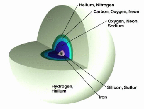
Figure 1.2: Schematic picture of the onion structure developed in a typical progenitor.

The Chandrasekhar limit is a stability criterion for compact objects like white dwarfs or the iron core of a massive star. Such objects are stabilized by electron degeneracy pressure. Depending on its mass, whether being above or below the Chandrasekhar limit, the star will follow different paths: $M<M_{\rm Ch}$, electrons become non-relativistic, stabilizing the star again; $M>M_{\rm Ch}$ (SN case), the degeneration of electrons cannot compensate the gravitational pressure and the star collapses.

1.2.2 Stellar core collapse

As soon as the last stage of nuclear burning begins at the center of the star, it starts developing a degenerate core formed by iron group elements, covered by a silicon crust. The iron core will continuously grow as the nuclear reactions at the border with the silicon layer add new material to it. Since the iron ignition will never occur this situation will not be stable for a long time. We have an inert sphere under a huge pressure, which is a configuration similar to that of a white dwarf. The stationary equilibrium is obtained thanks to the electron degeneration pressure, which is subjected to the Chandrasekhar limit, and is in this case around $1.2$–$1.5M_{\odot}$.
A) Start of the collapse
We end up then with an iron white dwarf of around $1.5M_{\odot}$, a central density of about $3.7\times 10^{9}$ g cm^-3, a central temperature of around $0.69$ MeV and an electron fraction (number of electrons per baryon) of $Y_{e}\simeq 0.42$. This last stage developes very fast and the iron core reaches the Chandrasekhar limit in days. At this point the electron degeneration pressure can no longer sustain the star and the collapse starts, lasting less than a second.

The rise in density and temperature originated by the collapse leads to new processes that accelerate the infall. There will be different processes involved, depending on the progenitor mass. The main ones are:

• Electron capture ($15$–$20M_{\odot}$). Due to the high densities attained during the collapse we will obtain electron capture by heavy elements,

  $$e^{-}(Z,A)\to\nu_{e}(Z-1,A)~{},$$ (1.1)

  such as,

  $${}^{24}{\rm Mg}+e^{-}\to~{}^{24}{\rm Na}+\nu_{e}~{},$$ (1.2)

  $${}^{56}{\rm Fe}+e^{-}\to~{}^{56}{\rm Mn}+\nu_{e}~{}.$$ (1.3)

  These processes have not only the effect of reducing the electron degeneration pressure by removing free electrons from the medium, but are also responsible for a huge energy loss in form of neutrinos. This is the first of the four neutrino emission phases.

• Nuclei photodissociation ($\gtrsim 20M_{\odot}$). In such massive stars the high temperatures reached make the iron nuclei photodissociation to be an important source of energy loss. The iron atoms are disintegrated in $\alpha$ particles due to the absorption of high energy photons,

  $${}^{56}{\rm Fe}+\gamma\to 13~{}^{4}{\rm He}+4n-124.4~{}{\rm MeV}~{}.$$ (1.4)

  The fast contraction of the star releases a big amount of gravitational energy, most of which is absorbed in the photodissociation of the iron atoms. Part of the energy required in these processes is obtained from the electrons, leading to a reduction of their pressure.

The net result in both cases is the acceleration of the collapse.
B) Neutrino trapping
We could say that the first stage of the collapse comes to an end when the density of the stellar core reaches a value of about $10^{12}$ g cm^-3. This is by no means the maximum density the core will register, since it continues to contract. Nevertheless, it marks an important point in the SN evolution: at this density matter becomes opaque to neutrinos, contrary to the initial moments of the collapse, where neutrinos can freely escape the star. The dominant opacity source for neutrinos in the collapse is neutral current interactions with heavy elements. The coherent scattering cross section for these processes is proportional to $A^{2}$.

The confinement is not permanent and after several interactions the neutrino would eventually escape the core. The diffusion time, though, is longer than the dynamic time of the collapse, leading to an effective confinement. One can define the neutrino sphere ($R_{\nu}$) as the surface where the optical depth of neutrinos, $\int_{r}^{\infty}\lambda_{\nu}^{-1}{\rm d}r^{\prime}$, becomes unity. This radius is shown in Fig. 1.4 as a function of time with a dotted line. One can approximately consider the region inside the neutrino sphere opaque to neutrinos and the exterior transparent.

The main consequences of the neutrino trapping are:

• Lepton fraction conservation, $Y_{L}=Y_{e}+Y_{\nu}\simeq 0.35$, during the collapse. Once neutrinos are trapped, they become degenerate, as the electrons, and reach $\beta$ equilibrium,

  $$e^{-}+p\longleftrightarrow n+\nu_{e}~{}.$$ (1.5)

• Change in the nuclear state. The degeneration of neutrinos leads to a suppression of the neutronization process (protons convert to neutrons through electron capture), since the neutrino emission derived from it is forbidden by the Pauli exclusion principle. Therefore heavy nuclei do not melt into free nucleons until the density approaches the nuclear density.

C) Core bounce and shock wave formation
The electron captures produced at the first stages of the collapse will not only reduce the electron degeneration pressure but also the electron fraction, and therefore $M_{\rm Ch}$. On the other hand, there is a change in the role played by this parameter in the SN dynamics. While initially it represented the largest amount of mass that could be supported by the electron pressure, it now becomes the largest amount of mass that can collapse homologously. As a consequence the collapsing core is considered to be composed of two parts (stage 1 of Fig. 1.3):

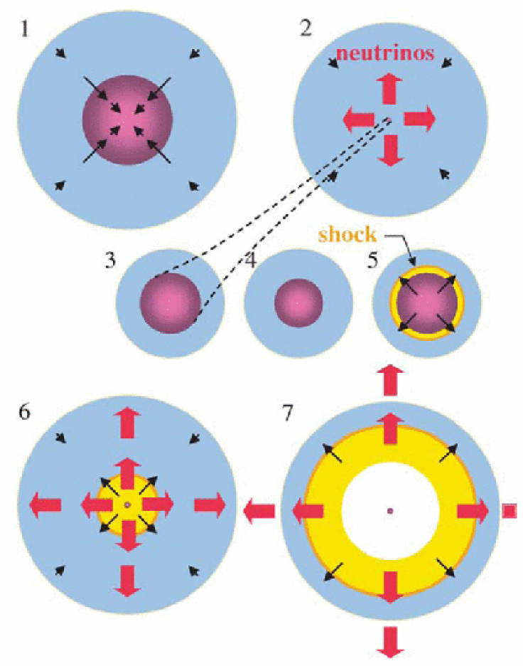
Figure 1.3: Different stages of the SN evolution. The core separates into an inner, subsonically collapsing core and an outer, supersonically collapsing core. When the core is no longer compressible it bounces, generating a shock wave which propagates outwards and ultimately will produce the SN explosion [27].

• inner core ($R_{\rm ic}$ in Fig. 1.4), collapsing homologously and subsonically.

• outer core ($R_{\rm Fe}$ in Fig. 1.4), collapsing supersonically in a free fall.

Figure 1.4: Schematic picture of stellar core collapse, formation of the neutron star remnant and the start of the SN explosion. The figure shows particular radial positions in the star’s central region as they evolve in time. The evolution can be divided in four stages: 1. collapse phase, 2. neutronization burst, 3. matter accretion phase, 4. protoneutron star cooling phase. $R_{\rm Fe}$ is the radius of the stellar iron core, $R_{\rm ic}$ is the inner core, $R_{\nu}$ is the neutrino sphere and $R_{\rm shock}$ indicates the shock wave position [28].

The collapse continues and the central density keeps growing until nuclear matter densities are reached ($\sim 1$–$3\times 10^{14}$ g cm^-3). At this point the nucleons and nuclei in the inner core merge to form a macroscopic state of nuclear matter. Due to Fermi effects and the repulsive nature of the nucleon-nucleon interactions at short distances, there is a dramatic rise in pressure. Consequently the inner core becomes incompressible and rebounds (stages 3–5 of Fig. 1.3). The core bounce generates sound waves that start propagating radially out of the inner core. They will not get very far though, since the material in the outer core is falling supersonically, forcing them to accumulate at the sonic point (border between the subsonically infalling inner core and the supersonically infalling outer core). The net effect is the formation of a density, pressure, and velocity discontinuity in the flow, i.e., a shock wave, which acquires more and more energy and almost immediately propagates to the outer part of the iron core.

1.2.3 Deleptonization and cooling

A) Neutronization burst
Once the core bounces and the shock wave is created, it starts propagating outwards, dissociating nuclei into free nucleons (stages 5–7 of Fig. 1.3). Since the electron capture cross section on free protons is larger than the one on nuclei, an enormous amount of electron neutrinos are created through the neutronization reaction $e^{-}+p\to n+\nu_{e}$, in those regions affected by the shock wave. As already explained, neutrinos are initially trapped due to the large density of the medium. The situation changes when the shock wave gets to the neutrino sphere dissociating the iron nuclei, some of the pressure is relieved and neutrinos can freely escape. This sudden neutrino emission leads to a momentary rise in the luminosity up to $10^{54}$ erg s^-1, known as neutronization burst or prompt neutrino burst, and constitutes the second stage of the neutrino emission. The duration of this peak is $\lesssim 10$ ms, and is shown in Fig. 1.6.

The two processes here described, namely nuclei dissociation and neutrino emission, are responsible for an energy loss in the shock wave which gets stalled in the iron core at a few hundred km. Its revival is one of the most important issues currently discussed in the theory of gravitational core collapse SNe.
B) Matter accretion and mantle cooling

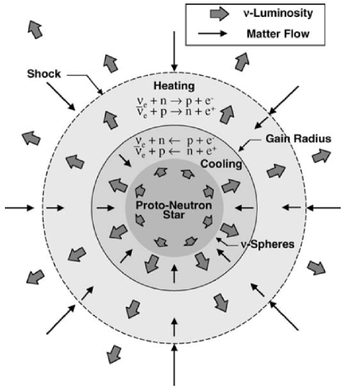
Figure 1.5: Schematic representation of the exploding star after the shock wave passage in the reheating phase. Below the neutrino sphere we have the central radiating proto-neutron star while above it, but below the stalled shock wave, there is a net cooling region and a net heating region, mediated by electron neutrino and antineutrino absorption and emission [27].

At this point the situation is as represented in Fig. 1.5. Under the shock wave remains a central radiating object, the proto-neutron star (PNS), which will go on to form a neutron star or a black hole. The PNS has a relatively cold inner part, below the point where the shock wave was formed, composed of neutrons, protons, electrons and neutrinos ($Y_{L}\simeq 0.35$). Surrounding this region there is a hot mantle formed by “shocked” nuclear material with low lepton number.

Since this mantle is hot ($T\gtrsim\mathcal{O}(10)$ MeV) and has a relatively low density, the electrons are not quite degenerate and relativistic thermal positrons can be created. Their presence will give rise to the appearance of neutrinos through $e^{+}+n\to\bar{\nu}_{e}+p$ and $e^{+}+e^{-}\to\nu+\bar{\nu}$ reactions. This point marks the third phase in the neutrino emission. In contrast to the neutronization burst, where only electron neutrinos are emitted, here all three flavors of neutrinos and antineutrinos are created and emitted as the mantle cools and contracts in the Kelvin-Helmholtz cooling phase.

On top of that, the external core accretes material over the PNS. The gravitational energy released in this process is transformed into thermal energy and emitted as thermal neutrinos. This stage lasts between 10 ms and 1 s, and the neutrino luminosities remain in an average value of $\sim 10^{52}$ erg s^-1 thanks to the accreted material. We therefore obtain that the cooling and the neutronization/deleptonization take place for the shocked outer regions earlier than for the inner regions.
C) Proto-neutron star
In this stage (also known as Kelvin-Helmholtz cooling phase), the part of the star that has not been ejected during the explosion evolves from a hot and lepton rich configuration (PNS) to a cold and deleptonized neutron star.

This stage represents the fourth and last of the neutrino emission phases. Once the explosion starts, after the accretion phase, there is a dramatic decrease in luminosity. As shown in Fig. 1.6, we observe an exponential fall in the neutrino luminosity characteristic of the neutron star formation and its cooling.

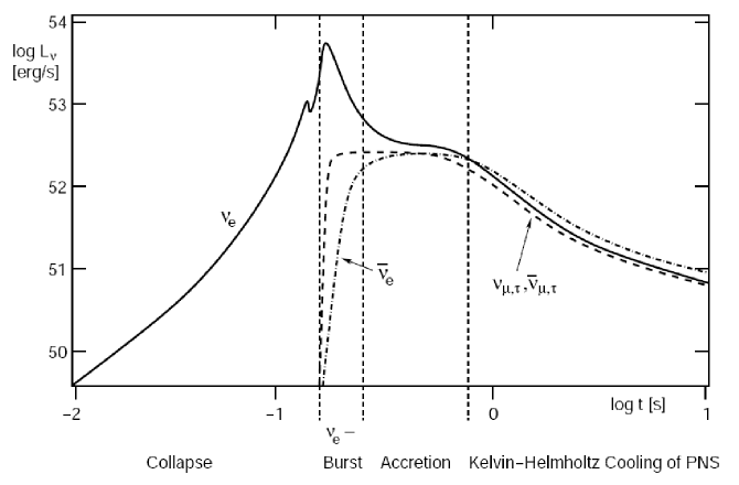
Figure 1.6: Schematic neutrino luminosity curves for the different emission phases, corresponding to $\nu_{e}$ (solid line), $\bar{\nu}_{e}$ (dot-dash line) and each of the non-electron neutrinos (dashed line) [29].

1.2.4 Supernova Explosion

The simplest scenario for a SN to take place would be that where the shock wave has enough energy to go beyond all the infalling material and blow up the star. In less than a second it would leave the iron core and a moment later would eject the remaining outer layers, producing a purely hydrodynamical explosion in a time scale of about 10 ms. This is the so called prompt explosion scenario [30] and in order to be successful one needs a sufficiently small and cold core and a soft equation of state. Nevertheless, in general, numerical simulations do not seem to confirm such a simple scenario as the one chosen by nature to carry out the final SN explosion.

The shock wave undergoes a series of processes, resulting in energy losses which progressively weakens it and ultimately stops its progression. On the other hand SNe are not a theoretical hypothesis, but take place in the Universe. This is why a lot of effort has been focused in determining the way the shock wave is revived and the explosion is obtained in the delayed mechanism.

Different ingredients are being considered as possible contributions to the phenomenon, and a combination of them may actually be involved in the SN explosion mechanism: heating of the postshock region by neutrinos, multi-dimensional hydrodynamic instabilities of the accretion shock, in the postshock region, and in the PNS, rotation, PNS pulsations, magnetic fields, and nuclear burning.

Three SN explosion mechanisms are centering nowadays the discussion [31]:

• The neutrino mechanism, where the shock wave is reactivated by the electron neutrinos and antineutrinos coming out the PNS. Part of these are absorbed by protons and neutrons behind the shock wave, providing the energy required. This mechanism was proposed by Wilson and Bethe [32], and although the energy released in form of neutrinos is by far larger than the energy needed to drive the explosion, it is very difficult to clarify the role played by the neutrino heating in the SN explosion mechanism.

• The magneto-rotational or magneto-hydrodynamic (MHD) [33, 34] mechanism, where the needed energy would be obtained from the rapid rotation of the collapsing stellar core and the amplification of magnetic fields through compression and wrapping. Such scenarios seem plausible in the cases of hypernovae, leading to jet-like explosions, but are disfavored for ordinary SNe because of the slow rotation of their progenitors predicted by stellar evolution calculations.

• The acoustic mechanism, recently proposed by Burrows et al. [35, 36], relies on the acoustic power generated in the core of the PNS. According to this mechanism, the energy produced in the large-amplitude core motions would be transported via strong sound waves to the postshock region and deposited there, eventually triggering the late explosions at $\gtrsim$ 1 s after bounce. This mechanism appears to be sufficiently robust to blow up even the most massive and extended progenitors, but has so far not been confirmed by other groups. Although the acoustic modes are also found in other numerical simulations, like the ones performed by the Garching group [31], their amplitude seem to be much smaller, leading to no practical effects.

1.3 Expected neutrino signal

Independently of the concrete SN explosion mechanism, presumably there are several characteristics regarding neutrinos that must result from such an event. Let us here review the most important ones.

1.3.1 General properties

The energy released in such an event comes from the gravitational binding energy of the compact star born after the collapse

$$E_{\rm b}=\Delta E_{\rm G} = -\frac{3}{5}\left(\frac{G_{\rm N}M_{\rm core}^{2}}{R_{\rm Fe~{}core}}-\frac{G_{\rm N}M_{\rm core}^{2}}{R_{\rm Neutron~{}star}}\right)$$ (1.6)

$$\approx 1.60\times 10^{53}{\rm erg}\left(\frac{M_{\rm core}}{M_{\odot}}\right)^{2}\left(\frac{10~{}{\rm km}}{R_{\rm NS}}\right)~{}.$$

It seems reasonable to assume approximate equipartition of this energy among the different neutrino flavors, receiving $E_{\rm b}/6$ each of the 6 degrees of freedom that conform the standard (anti)neutrinos.

These neutrinos are trapped inside the PNS due to its huge density, being released only after several collisions from a surface of $r\approx 10$–$20$ km. The gravitational pressure of this compact object is sustained by the thermal pressure, as long as matter near its surface is not degenerate. We can make use of the virial theorem in order to obtain the mean kinetic energy of a typical nucleon near the PNS surface,

$$\langle E_{\rm kin}\rangle=-\frac{1}{2}\langle E_{\rm G}\rangle\approx\frac{1}{2}G_{\rm N}\frac{Mm_{\rm N}}{R}~{},$$ (1.7)

leading to a typical value for the temperature of order 10 MeV, which will therefore characterize the thermal neutrinos released.

As for the duration of the emission, it should be a multiple of the typical diffusion time,

$$t_{\rm diff}\approx R_{\rm NS}^{2}/\lambda~{},$$ (1.8)

where $\lambda$ stands for the mean free path. In order to give an estimate of $t_{\rm diff}$ we use the scattering cross section off non-relativistic nucleons, $\sigma\approx G_{F}^{2}E_{\nu}^{2}/\pi=1.7\times 10^{-42}$ cm${}^{2}(E_{\nu}/10~{}{\rm MeV})^{2}$ and an approximate density of $\rho_{0}\approx 3\times 10^{14}$ g cm^-3. Using characteristic values of the involved quantities we obtain a $\lambda\approx 300$ cm for neutrinos of 30 MeV, which leads to a diffusion time of order $t_{\rm diff}=\mathcal{O}(1~{}{\rm s})$.

1.3.2 Energies and spectra

We have then some generic features of neutrinos coming out of the SN core, confirmed by numerical simulations of neutrino transport. Furthermore it is obvious that the nature of the scenario we are dealing with will give rise to substantial differences among neutrino flavors. Let us try to analyze some of them.

On top of the average neutrino energy of 10 MeV previously motivated, all numerical simulations seem to obtain the same hierarchy for the specific flavor average energies. According to the simulations, electron neutrinos would start their free streaming above the neutrino sphere with a lower average energy than electron antineutrinos, which in turn have a lower average energy than muon and tau (anti)neutrinos, $\langle E_{\nu_{e}}\rangle\lesssim\langle E_{\bar{\nu}_{e}}\rangle\lesssim\langle E_{\nu_{x}}\rangle$ ($\nu_{x}\equiv\nu_{\mu},\nu_{\tau},\bar{\nu}_{\mu},\bar{\nu}_{\tau}$). This can be understood by using some simple arguments.

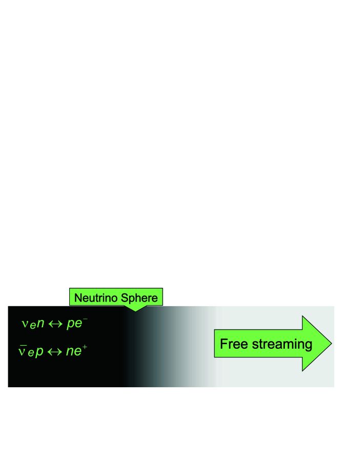
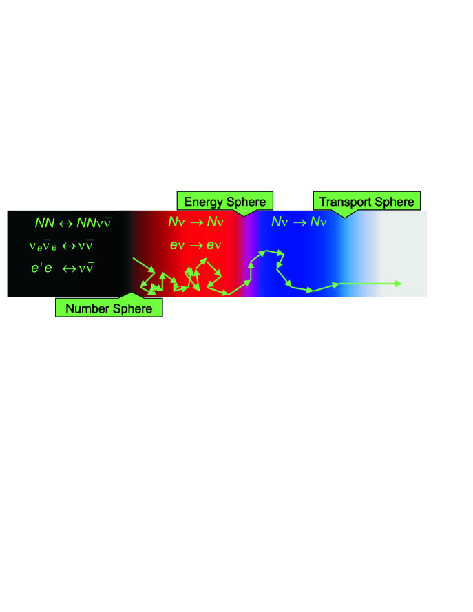
Figure 1.7: Schematic representation of the neutrino evolution through the star, showing the different neutrino spheres. The top panel correspond to $\nu_{e}$ and $\bar{\nu}_{e}$ and the bottom one to non-electron neutrinos [37].

The top panel of Fig. 1.7 shows schematically the propagation of $\nu_{e}$ and $\bar{\nu}_{e}$ throughout the SN. The main reactions responsible for keeping them trapped inside the core in thermal equilibrium are $\beta$ processes: neutron capture and proton capture, respectively. The energy dependence of these reactions is exactly the same, leading in principle to equal energy spectra for both types of neutrinos. Nevertheless, this is not the whole story, since the core of the star, in its way of becoming a neutron star, contains more neutrons than protons, and this difference will only grow with time. As a consequence $\nu_{e}$’s have a higher absorption rate than $\bar{\nu}_{e}$’s, which is translated into a deeper $\nu_{e}$ neutrino sphere. The radius where neutrinos decouple from the PNS will determine their energy, higher radius means lower densities and temperatures. Since this argument applies for all neutrino energies, the mean energy of the emitted $\bar{\nu}_{e}$ will always be larger than the mean energy of the $\nu_{e}$.

Concerning the remaining part of the energy hierarchy relation, the bottom panel of Fig. 1.7 shows schematically the non-electron neutrino transport. Since there are no $\mu$ nor $\tau$ leptons in the medium and therefore $\nu_{x}$ neutrinos do not experience charged currents, we would naively expect them to decouple deeper inside the PNS, compared to electron flavor neutrinos. The situation is a bit more complicated though. It is true that there are no charged current interactions for $\nu_{x}$, but they suffer from a variety of neutral currents that must be taken into account. According to the dominant interactions taking place we can distinguish four regimes of evolution separated by different spheres: number sphere, energy sphere and transport sphere.

In the innermost region the non-electron neutrinos are kept in thermal equilibrium by energy exchanging scattering processes and the following pair processes: Bremsstrahlung $NN\leftrightarrow NN\nu\bar{\nu}$, neutrino-pair annihilation $\nu_{e}\bar{\nu}_{e}\leftrightarrow\nu\bar{\nu}$ and electron-positron-pair annihilation $e^{+}e^{-}\leftrightarrow\nu\bar{\nu}$. The radius where these interactions become inefficient defines the number sphere.

Beyond this point $\nu_{x}$’s are no longer in thermal equilibrium, although they still exchange energy with the medium via scattering reactions: $N\nu\to N\nu$ and $e^{\pm}\nu\to e^{\pm}\nu$. However, the two processes are qualitatively very different. Scattering on e^± is less frequent since the interaction cross section is smaller and there are fewer e^± than nucleons. On the other hand the amount of energy exchanged in each interaction with e^± is very large compared to the small recoil of nucleons. At the radius, where scattering on e^± freezes out lies the energy sphere. A diffusive regime starts, where neutrinos only scatter on nucleons and therefore exchange little energy in each reaction. This regime is terminated by the transport sphere, defined by the radius at which also scattering on nucleons becomes ineffective and the $\nu_{x}$ start streaming freely.

Due to its dependence on the square of neutrino energy the nucleon scattering cross section has a filter effect, because it tends to scatter high energy neutrinos more frequently [38]. The position of the number sphere determines the flux, because neutrino creation is not effective beyond that radius. The $\nu_{x}$ flux that passes the number sphere is conserved. On the other hand, the mean energy of $\nu_{x}$ in this area is still significantly lowered due to scattering processes before the $\nu_{x}$ leave the star. The mean energy of $\nu_{x}$ emerging the star is usually found to be larger than that of $\bar{\nu}_{e}$.

Typical values for the mean energies obtained in numerical simulations are:

$$\langle E_{\nu}\rangle=\left\{\begin{array}[]{cl}10\mbox{--}12~{}{\rm MeV}&\nu_{e}\\ 14\mbox{--}18~{}{\rm MeV}&\bar{\nu}_{e}\\ 18\mbox{--}24~{}{\rm MeV}&\nu_{\mu,\tau},\bar{\nu}_{\mu,\tau}\\ \end{array}\right.$$ (1.9)

As for the number fluxes, there is again a hierarchy relation among them. The non-electron flavor ones are smaller than those of $\bar{\nu}_{e}$ because the energy is found to be approximately equipartitioned between the flavors. Similarly, since the lepton number is carried away in $\nu_{e}$’s, their number flux is larger than that of $\bar{\nu}_{e}$, so that again the energy is approximately equipartitioned between $\nu_{e}$ and $\bar{\nu}_{e}$. In summary, we obtain the hierarchy in the number fluxes: $F_{\nu_{e}}>F_{\bar{\nu}_{e}}>F_{\nu_{x}}=F_{\bar{\nu}_{x}}$.

Throughout the literature one can find different forms of parameterizing the non-thermal spectra of the neutrino fluxes. Two of them are the most used. The first one is the quasi Fermi-Dirac distribution:

$$F^{0}_{\nu}(E)=\frac{\Phi_{\nu}}{T_{\nu}^{3}f_{2}(\eta_{\nu})}\frac{E^{2}}{e^{E/T_{\nu}-\eta_{\nu}}+1},$$ (1.10)

where $E$ is the neutrino energy, and $T_{\nu}$ and $\eta_{\nu}$ denote an effective temperature and degeneracy parameter (chemical potential), respectively. The distribution is normalized so that $\Phi_{\nu}$ stands for the total number of $\nu$ emitted. The function $f_{n}(\eta_{\nu})$ is defined as

$$f_{n}(\eta_{\nu})\equiv\int_{0}^{\infty}\frac{x^{n}}{{\rm e}^{x-\eta_{\nu}}+1}{\rm d}x\,.$$ (1.11)

The mean energy is consequently $\langle E_{\nu}\rangle=\left[f_{3}(\eta_{\nu})/f_{2}(\eta_{\nu})\right]T_{\nu}$, and the total energy released is $E_{\nu}^{\rm tot}=\Phi_{\nu}\langle E_{\nu}\rangle$.

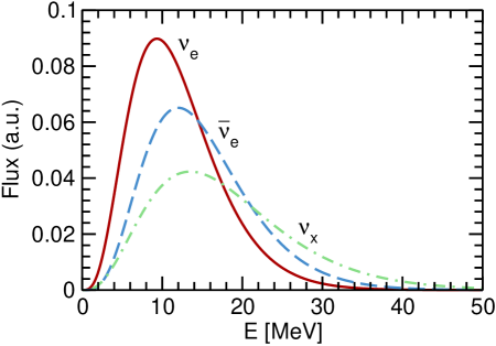
Figure 1.8: Neutrino fluxes given by Eq. (1.12), with $\langle E_{\nu_{e}}\rangle=12$, $\langle E_{\bar{\nu}_{e}}\rangle=15$, $\langle E_{\nu_{x}}\rangle=18$, $\alpha_{\nu_{e}}=3.5$, $\alpha_{\bar{\nu}_{e}}=4$ and $\alpha_{\nu_{e}}=3$. The flux is given in arbitrary units (a.u.) so that $\Phi_{\nu_{e}}=1.15$, $\Phi_{\bar{\nu}_{e}}=1$ and $\Phi_{\nu_{x}}=0.85$.

The second parametrization, shown in Fig. 1.8, has been recently introduced by the Garching group and fits better their numerical results [37]:

$$F^{0}_{\nu}(E)=\frac{\Phi_{\nu}}{\langle E_{\nu}\rangle}\,\frac{(1+\alpha)^{1+\alpha}}{\Gamma(1+\alpha)}\left(\frac{E}{\langle E_{\nu}\rangle}\right)^{\alpha}\exp\left[-(\alpha+1)\frac{E}{\langle E_{\nu}\rangle}\right]\,,$$ (1.12)

where $\alpha$ describes a possible deformation with respect to a Fermi-Dirac distribution.

Fig. 1.9 shows a numerical simulation where we can see the mean energies (denoted by $\epsilon$) and the luminosities. In this simulation we can identify all the features we have been discussing in this section.

Figure 1.9: Numerical result of the first two seconds after the core rebound. Top left: Only the mean energy of the $\nu_{e}$’s is affected by the neutronization burst. Top right: The evolution of the mean energies shows the hierarchy discussed in the text. Bottom left: The neutronization explosion lasts for a few ms. Bottom right: Temporal evolution of luminosities [39].

Chapter 2 Standard Neutrino Oscillations

In the last years, it has been widely demonstrated that neutrinos oscillate from one flavor to another. This phenomenon occurs when the interaction and mass bases do not coincide, meaning that the particles which propagate are not the same as the ones that are created or detected. This has been proven to be the case for neutrinos, created via charged current weak interactions as one of the weak eigenstates $\nu_{e}$, $\nu_{\mu}$ and $\nu_{\tau}$, different in general from the propagating mass eigenstates $\nu_{1}$, $\nu_{2}$ and $\nu_{3}$, since the mass matrix in the flavor basis is not diagonal. This, as we will later show, leads inevitably to neutrino oscillations.

The first one to address the question of oscillation in the neutrino system was Pontecorvo [40] in 1957. Inspired in the well known $K^{0}\leftrightarrow\bar{K}^{0}$ oscillations, Pontecorvo initially proposed neutrino-antineutrino oscillations. The precise realization of the idea in terms of mass and mixing was introduced by Maki, Nakagawa and Sakata [41] in 1962 and later developed by Pontecorvo [42] in 1967.

This phenomenon will affect neutrino propagation through the SN envelope and therefore has to be taken into account when studying SN neutrinos. This problem can be attacked in two different ways. Either we assume we have under control the part involving neutrino properties (masses, mixing and CP-violating phases) and try to learn about SN physics (explosion dynamics, SN neutrino fluxes and spectra, etc), or we assume we have a good enough understanding of the SN physics and try to improve our knowledge on the neutrino parameters. Throughout this thesis we will mainly follow this second approach, trying to gain some insight in the neutrino properties, by making some assumptions in the SN models.

In this chapter we will introduce the basics of neutrino oscillations in different steps. We will first treat vacuum oscillations in two and three neutrino scenarios. After that we will discuss the effect of neutrino interactions with matter, starting with a constant density medium and later consider the varying density case. Finally we will apply the formalism discussed in these sections to analyze the evolution of neutrinos through SN envelopes.

2.1 Vacuum oscillations

The problem we want to discuss is the probability of observing a neutrino flavor eigenstate different than the one created after a certain time. While the natural basis to study neutrino interactions is the flavor one, their evolution in vacuum is much simpler in the mass eigenstate basis. We can always define a unitary transformation, linking both neutrino basis and express the flavor eigenstates $\nu_{\alpha}$ ($\alpha=e,\mu,\tau$) as a linear combination of the mass eigenstates $\nu_{i}$ ($i=1,2,3$),

$$|\nu_{\alpha}\rangle=U^{*}_{\alpha i}\,|\nu_{i}\rangle\,,$$ (2.1)

where we are summing over repeated indexes up to the number of neutrino species. The relation for antineutrinos is exactly the same but complex conjugating the elements in the mixing matrix $U$, i.e. $|\bar{\nu}_{\alpha}\rangle=U_{\alpha i}\,|\bar{\nu}_{i}\rangle\,$. Therefore, only for a complex $U$ (including a CP violating phase) we would observe a difference in the evolution of neutrinos and antineutrinos in vacuum.

Using Eq. (2.1), the initial neutrino state at $t=0$ can be written as $|\nu(0)\rangle=|\nu_{\alpha}\rangle=U^{*}_{\alpha i}|\nu_{i}\rangle$. After a time $t$ the mass eigenstates just acquire a phase, leading to

$$|\nu(t)\rangle=U^{*}_{\alpha i}\,e^{-iE_{i}t}|\nu_{i}\rangle\,.$$ (2.2)

If we now project this state onto a flavor eigenstate we find the probability amplitude of finding the initial neutrino in that particular state,

$$A(\nu_{\alpha}\to\nu_{\beta})=\langle\nu_{\beta}|\nu(t)\rangle=U^{*}_{\alpha i}\,e^{-iE_{i}t}\,\langle\nu_{\beta}|\nu_{i}\rangle=U_{\beta j}U^{*}_{\alpha i}\,e^{-iE_{i}t}\,\langle\nu_{j}|\nu_{i}\rangle=U_{\beta i}\,e^{-iE_{i}t}\,U^{*}_{\alpha i}\,.$$ (2.3)

And finally, squaring this amplitude we obtain what we were looking for, the probability of finding $|\nu_{\beta}\rangle$ at $t$ when creating $|\nu_{\alpha}\rangle$ at $t=0$,

$$P(\nu_{\alpha}\to\nu_{\beta})=|A(\nu_{\alpha}\to\nu_{\beta})|^{2}=|U_{\beta i}\,e^{-iE_{i}t}\,U^{*}_{\alpha i}|^{2}\,.$$ (2.4)

Expanding this last expression we obtain

$$P(\nu_{\alpha}\to\nu_{\beta})=\sum_{i}|U_{\beta i}|^{2}|U^{*}_{\alpha i}|^{2}+2{\rm Re}\left[\sum_{i\neq j}U_{\beta i}U^{*}_{\alpha i}U^{*}_{\beta j}U_{\alpha j}\,e^{-i(E_{i}-E_{j})t}\right]\,,$$ (2.5)

where we have explicitly written the summation. In all cases of interest to us, the neutrinos are relativistic, so that we can approximate,

$$E_{i}=\sqrt{p^{2}+m_{i}^{2}}\simeq p+\frac{m_{i}^{2}}{2p}\simeq p+\frac{m_{i}^{2}}{2E}\,,$$ (2.6)

and rewrite Eq. (2.5) as

$$P(\nu_{\alpha}\to\nu_{\beta})=\sum_{i}|U_{\beta i}|^{2}|U^{*}_{\alpha i}|^{2}+2{\rm Re}\left[\sum_{i\neq j}U_{\beta i}U^{*}_{\alpha i}U^{*}_{\beta j}U_{\alpha j}\,e^{-i\frac{\Delta m^{2}_{ij}}{2E}t}\right]\,,$$ (2.7)

in terms of the neutrino squared mass differences, $\Delta m^{2}_{ij}=m^{2}_{i}-m^{2}_{j}$.

2.1.1 Two flavor case

Let us take a closer look at Eq. (2.7) in the two flavor scenario, i.e. we will only consider for the moment $\nu_{e}$ and $\nu_{\mu}$. The mixing matrix connecting the flavor and interaction basis takes the simple form

$$U=\left(\begin{array}[]{cc}\cos\theta_{0}&\sin\theta_{0}\\ -\sin\theta_{0}&\cos\theta_{0}\end{array}\right)\,,$$ (2.8)

where $\theta_{0}$ is the mixing angle. Making use of Eqs. (2.7) and (2.8) we obtain the oscillation probabilities in two flavors

$$P(\nu_{e}\to\nu_{\mu})=P(\nu_{\mu}\to\nu_{e})=\sin^{2}2\theta_{0}\,\sin^{2}\left(\frac{\Delta m^{2}}{4E}L\right)\,,$$ (2.9)

where $\Delta m^{2}=m_{2}^{2}-m_{1}^{2}$ and $L\simeq t$ (for relativistic neutrinos) is the distance between the source and the detector. Unitarity assures that the survival probabilities are $P(\nu_{e}\to\nu_{e})=P(\nu_{\mu}\to\nu_{\mu})=1-P(\nu_{e}\to\nu_{\mu})$. Since $U$ is real in the two flavor scenario, the same expressions are obtained for antineutrino survival and oscillation probabilities. Another convenient way of expressing the transition probability is given by

$$P(\nu_{e}\to\nu_{\mu})=\sin^{2}2\theta_{0}\,\sin^{2}\left(1.27\Delta m^{2}\frac{L}{E}\right)\,,$$ (2.10)

where $L$ is in m and $E$ in MeV or $L$ is in km and $E$ in GeV.

There are several remarkable features in these expressions. The first one is the oscillatory behavior in $L/E$, explaining why we call them neutrino oscillations. In Eq. (2.9) we can distinguish two factors: a constant amplitude, $\sin^{2}2\theta_{0}$, and an oscillatory term, $\sin^{2}(\frac{\Delta m^{2}}{4E}L)$. If we first focus in the amplitude we note that a non-zero mixing angle is required to obtain oscillations. On the other extreme, the maximum in the amplitude corresponds to a mixing angle of $\theta_{0}=45^{\circ}$, maximal mixing. Paying now attention to the oscillatory term we observe that no flavor transitions would occur for massless neutrinos. Summarizing, neutrino oscillations require both mass and mixing to take place.

Furthermore, $(\Delta m^{2}/4E)L$ must be of order unity if we want to observe the oscillatory pattern. We can explicitly define the oscillation length,

$$L_{osc}=\frac{4\pi E}{\Delta m^{2}}\,\simeq\,2.48\;{\rm m}\,\frac{E\,\mbox{(MeV)}}{\Delta m^{2}\,(\mbox{eV}^{2})}=\,2.48\;{\rm km}\,\frac{E\,\mbox{(GeV)}}{\Delta m^{2}\,(\mbox{eV}^{2})}\,,$$ (2.11)

which will help us in this argument. For $L\ll L_{osc}$ no oscillations have developed yet, the phase in Eq. (2.9) is very small, leading to no visible effect. On the other hand, for a very large phase, $L\gg L_{osc}$, the transition probability experiences very fast oscillations, translated at the detector in the averaged probability over distance

$$\overline{P(\nu_{e}\to\nu_{\mu})}=\overline{P(\nu_{\mu}\to\nu_{e})}=\frac{1}{2}\,\sin^{2}2\theta_{0}\,.$$ (2.12)

It is also remarkable how the oscillation probability depends on the neutrino mass, through the squared mass splittings $\Delta m^{2}$. The unfortunate consequence is that it will not be possible to access the information about the absolute individual neutrino masses through oscillation experiments, but only the squared mass differences.

2.1.2 Three flavor case

The number of active neutrino species can be indirectly determined through the invisible width of the $Z^{0}$ decay [43]. LEP measured experimentally this quantity, obtaining $N_{\nu}=2.984\pm 0.008$, and proving the existence of only three active neutrino flavors, $\nu_{e}$, $\nu_{\mu}$ and $\nu_{\tau}$. In the three-neutrino scenario the flavor eigenstates are related to the mass eigenstates through

$$\left(\begin{array}[]{c}\nu_{e}\\ \nu_{\mu}\\ \nu_{\tau}\end{array}\right)=\left(\begin{array}[]{ccc}U_{e1}&U_{e2}&U_{e3}\\ U_{\mu 1}&U_{\mu 2}&U_{\mu 3}\\ U_{\tau 1}&U_{\tau 2}&U_{\tau 3}\end{array}\right)\left(\begin{array}[]{c}\nu_{1}\\ \nu_{2}\\ \nu_{3}\end{array}\right)\,.$$ (2.13)

The simplest unitary form of the lepton mixing matrix, for the case of Dirac neutrinos, is given in terms of three mixing angles $\theta_{12}$, $\theta_{13}$ and $\theta_{23}$ and one CP-violating phase, $\delta$. The case of Majorana neutrinos is slightly more complicated, adding two more phases, $\varphi_{1}$ and $\varphi_{2}$, although they will not affect neutrino oscillations. The resulting leptonic mixing matrix $U$, also known as PMNS matrix, can be factorized following e.g. the Particle Data Group [43], into four different matrices,

$${U=V_{23}W_{13}V_{12}D\equiv VD\,,}$$ (2.14)

with

$${V_{12}=\left(\begin{array}[]{ccc}c_{12}&s_{12}&0\\ -s_{12}&c_{12}&0\\ 0&0&1\end{array}\right),~{}W_{13}=\left(\begin{array}[]{ccc}c_{13}&0&s_{13}\,e^{-i\delta}\\ 0&1&0\\ -s_{13}\,e^{i\delta}&0&c_{13}\end{array}\right),~{}V_{23}=\left(\begin{array}[]{ccc}1&0&0\\ 0&c_{23}&s_{23}\\ 0&-s_{23}&c_{23}\end{array}\right),}$$ (2.15)

where $c_{ij}=\cos\theta_{ij}$, $s_{ij}=\sin\theta_{ij}$, and $D={\rm diag}(e^{-i\varphi_{1}},\,1,\,e^{-i\varphi_{2}})$. Since the Majorana phases do not have any effect on neutrino oscillations, we can omit the $D$ factor, resulting in the following expression for Eq. (2.14)

$$U=\left(\begin{array}[]{ccc}c_{12}\,c_{13}&s_{12}\,c_{13}&s_{13}\,e^{-i\delta}\\ -s_{12}\,c_{23}-c_{12}\,s_{23}\,s_{13}\,e^{i\delta}&c_{12}\,c_{23}-s_{12}\,s_{23}\,s_{13}\,e^{i\delta}&s_{23}\,c_{13}\\ s_{12}\,s_{23}-c_{12}\,c_{23}\,s_{13}\,e^{i\delta}&-c_{12}\,s_{23}-s_{12}\,c_{23}\,s_{13}\,e^{i\delta}&c_{23}\,c_{13}\end{array}\right)\,.$$ (2.16)

Replacing this matrix into Eq. (2.7), we obtain the corresponding neutrino oscillation formulas in three flavors. Contrary to the two-flavor case, the neutrino and antineutrino formulas do not coincide, unless $\delta=0$ or $\pi$. Even though there are no simple expressions in this case, there are several approximations in terms of the two flavor ones, that apply for practical purposes, see for instance [44].

In the three-neutrino scenario there exist two independent squared mass differences, $\Delta m^{2}_{21}$ and $\Delta m^{2}_{31}$, that will determine the evolution of neutrinos, while $\Delta m^{2}_{32}$ can be easily reexpressed in terms of the other two.

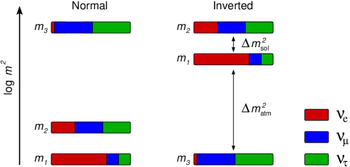
Figure 2.1: Possible neutrino mass hierarchy patterns. The left one shows the normal case, while the right one corresponds to inverted hierarchy. The colors show the amount of a given flavor eigenstate in each mass eigenstate, according to current best fits for the mixing angles.

2.1.3 Present status of three-flavor neutrino oscillations

Four of the six neutrino oscillation parameters are rather well determined by the oscillation data, the so called atmospheric ($|\Delta m^{2}_{31}|$, $\theta_{23}$) and solar ($\Delta m^{2}_{21}$, $\theta_{12}$) neutrino parameters, while $\theta_{13}$, $\delta$ and the sign of $\Delta m^{2}_{31}$ remain unknown [45, 6, 46, 47, 48].

The status of the atmospheric neutrino parameters is determined by the combination of different analyses. On the one hand, of course, we have the atmospheric neutrino measurements from Super-Kamiokande [49], which give the most stringent bound on the 23-mixing angle. On the other hand, the determination of $|\Delta m^{2}_{31}|$ is dominated by accelerator experiments, mainly MINOS data [50], while K2K [51] basically has no impact any more. The complementarity of these experiments leads to the following best fit point and $1\sigma$ errors [6]:

$$\sin^{2}\theta_{23}=0.50^{+0.07}_{-0.06}\,,\qquad|\Delta m^{2}_{31}|=2.40^{+0.12}_{-0.11}\times 10^{-3}\,{\rm eV^{2}}\,.$$ (2.17)

Although we have quite a good measurement of $|\Delta m^{2}_{31}|$, it is not possible to determine the hierarchy of neutrino masses, i.e. the sign of $\Delta m^{2}_{31}$, with the current data.

The determination of the solar neutrino parameters comes from the combination of KamLAND reactor experiment [52] and SNO [53], Super-Kamiokande [54], Borexino [55] and Gallex/GNO [56] solar neutrino experiments. Just as before, the determination of each parameter is dominated by one type of experiment. Thus, $\theta_{12}$ is mostly constrained by solar experiments (mainly SNO), while $\Delta m^{2}_{21}$ is basically determined by KamLAND. Nevertheless, KamLAND is also starting to help on the lower limit of $\theta_{12}$. The resulting parameters from this analysis are (at $1\sigma$) [6]:

$$\sin^{2}\theta_{12}=0.304^{+0.022}_{-0.016}\,,\qquad\Delta m^{2}_{21}=7.65^{+0.23}_{-0.20}\times 10^{-5}\,{\rm eV^{2}}\,.$$ (2.18)

Concerning the 13-mixing angle, at this moment we only have upper bounds coming from null results of the short-baseline CHOOZ reactor experiment [57] with some effect also from solar and KamLAND data, especially at low $\Delta m^{2}_{31}$ values. At 90% CL ($3\sigma$) the following limits are obtained [6]:

$$\sin^{2}\theta_{13}\leq\left\{\begin{array}[]{l@{\qquad}l}0.060~{}(0.089)&\text{(solar+KamLAND)}\\ 0.027~{}(0.058)&\text{(CHOOZ+atm+K2K+MINOS)}\\ 0.035~{}(0.056)&\text{(global data)}\end{array}\right.$$ (2.19)

Finally, no limit at all has been yet obtained for the CP violating phase in neutrino oscillation experiments.

From solar experiments we know that $\Delta m^{2}_{21}$, also known as solar squared mass difference ($\Delta m^{2}_{\rm sol}$), is positive, while the sign of $\Delta m^{2}_{31}$ or $\Delta m^{2}_{\rm atm}$, is yet unknown. This sign determines what is called the neutrino mass hierarchy, $\Delta m^{2}_{31}=|\Delta m^{2}_{31}|$ corresponds to normal hierarchy, and $\Delta m^{2}_{31}=-|\Delta m^{2}_{31}|$ to inverted hierarchy. As we will later see it will be crucial in the evolution of neutrinos inside the SN. Fig. 2.1 shows the two possible configurations for the hierarchy of neutrino masses.

A summary of the current knowledge of the neutrino parameters is given in Table 2.1. For a more detailed description of these fits see Refs. [6, 45].

parameter	best fit $\pm 1\sigma$	2$\sigma$	3$\sigma$
$\Delta m^{2}_{21}\>[10^{-5}{\rm eV^{2}}]$	$7.65^{+0.23}_{-0.20}$	7.25–8.11	7.05–8.34
$|\Delta m^{2}_{31}|\>[10^{-3}{\rm eV^{2}}]$	$2.40^{+0.12}_{-0.11}$	2.18–2.64	2.07–2.75
$\sin^{2}\theta_{12}$	$0.304^{+0.022}_{-0.016}$	0.27–0.35	0.25–0.37
$\sin^{2}\theta_{23}$	$0.50^{+0.07}_{-0.06}$	0.39–0.63	0.36–0.67
$\sin^{2}\theta_{13}$	$0.01^{+0.016}_{-0.011}$	$\leq$ 0.040	$\leq$ 0.056

Table 2.1: Best-fit values with 1$\sigma$ errors, and 2$\sigma$ and 3$\sigma$ intervals (1 d.o.f.) for the three-flavor neutrino oscillation parameters from global data, including solar, atmospheric, reactor (KamLAND and CHOOZ) and accelerator (K2K and MINOS) experiments [6].

2.2 Neutrino oscillations in matter

In most experiments, neutrinos travel through matter before being detected. Solar neutrinos are emitted from deep inside the Sun and have to travel not only through it before hitting the detector but also through part of the Earth at night. Geometry tells us that accelerator neutrinos must cross the Earth before being detected, as well as most of the atmospheric neutrinos, depending on the original interaction point. And of course the ones of most interest to us, SN neutrinos, which traverse the whole envelope of the star before finding vacuum. It is therefore of the utmost importance to determine the effect of matter in neutrino oscillations.

2.2.1 Neutrino interactions with matter

The Standard Model is built over the gauge group $SU(3)_{C}\otimes SU(2)_{L}\otimes U(1)_{Y}$, and describes the strong, weak and electromagnetic interactions of matter. According to this model, neutrinos are $SU(3)_{C}\otimes U(1)_{em}$ singlets, and therefore interact only via charged (CC) and neutral (NC) weak currents, described by the following Lagrangians:

$${\mathcal{L}}^{\rm CC} = \frac{g}{\sqrt{2}}\sum_{\alpha}\bar{e}_{\alpha L}\gamma^{\mu}\nu_{\alpha L}W_{\mu}^{-}+{\rm h.c.}~{},$$ (2.20)

$${\mathcal{L}}^{\rm NC} = \frac{g}{2\cos\theta_{W}}\sum_{\alpha}\bar{\nu}_{\alpha L}\gamma^{\mu}\nu_{\alpha L}Z_{\mu}^{0}~{},$$ (2.21)

where $g=e/\sin\theta_{W}$, with $e$ the electron charge and $\theta_{W}$ the weak angle, $f_{\alpha L}=\frac{1}{2}(1-\gamma_{5})f_{\alpha}$ correspond to the left-handed fermion fields, with $\alpha=e,\mu,\tau$, $\gamma^{\mu}$ are the Dirac matrices, and $W_{\mu}^{-}$ and $Z_{\mu}^{0}$ are the gauge boson fields.

The dominant source of neutrino interactions in a medium is coherent forward elastic scattering, under which the medium remains unchanged. As first discussed by Wolfenstein [9] in 1978, the effect of this coherent process on neutrinos can be parameterized as an effective potential affecting their evolution. Ordinary matter is composed of electrons, protons and neutrons, but not $\mu$ or $\tau$ leptons (in Chapter 4 we will study the effect of considering neutrinos as a background medium). As a consequence only $\nu_{e}$’s participate in CC mediated by the $W^{\pm}$ exchange, while all neutrino species have equal NC interactions on $n$, $p$ and $e^{-}$ mediated by $Z^{0}$ bosons, see Fig. 2.2.

Figure 2.2: Neutrino scattering diagrams.

Let us start by considering the effective potential induced by CC interactions. Its only contribution comes from elastic scattering of $\nu_{e}$’s on electrons, which in the effective low energy limit gives the following term to the interaction Hamiltonian,

$${\mathcal{H}}^{\rm CC}_{\rm eff} = \frac{G_{\rm F}}{\sqrt{2}}\{\bar{e}\gamma^{\mu}(1-\gamma_{5})\nu_{e}\}\{\bar{\nu}_{e}\gamma_{\mu}(1-\gamma_{5})e\}$$ (2.22)

$$= \frac{G_{\rm F}}{\sqrt{2}}\{\bar{\nu}_{e}\gamma^{\mu}(1-\gamma_{5})\nu_{e}\}\{\bar{e}\gamma_{\mu}(1-\gamma_{5})e\}~{},$$ (2.23)

where $G_{\rm F}/\sqrt{2}=g^{2}/8M_{W}^{2}$, and we have applied the Fierz rearrangement in the second line. The effective potential $V_{\rm CC}$ can be calculated as the matrix element of this interaction Hamiltonian:

$$V_{\rm CC}=\langle\Psi|{\mathcal{H}}^{\rm CC}_{\rm eff}|\Psi\rangle~{},$$ (2.24)

where $\Psi$ is the wave function of the system of neutrino and medium. We define the vector of polarization of electrons as

$$\vec{\lambda}_{e}\equiv\omega_{e}^{\dagger}\vec{\sigma}\omega_{e}~{},$$ (2.25)

where $\omega_{e}$ is the two component spinor. Suppose electrons have some density distribution over the momentum, $\vec{p}_{e}$ and polarization $\vec{\lambda}_{e}$:

$$\frac{f(\vec{\lambda}_{e},\vec{p}_{e})}{(2\pi)^{3}}~{}.$$ (2.26)

Then the total number density of electrons, $N_{e}$, equals

$$N_{e}=\sum_{\vec{\lambda}}\int\frac{d^{3}p_{e}}{(2\pi)^{3}}~{}f(\vec{\lambda_{e}},\vec{p}_{e})~{}.$$ (2.27)

The average polarization of electrons is defined as

$$\langle\vec{\lambda}_{e}\rangle=\frac{1}{N_{e}}\ \sum_{\vec{\lambda}}\int\frac{d^{3}p_{e}}{(2\pi)^{3}}\vec{\lambda}~{}f(\vec{\lambda}_{e},\vec{p}_{e})~{}.$$ (2.28)

The matrix element of Eq. (2.24) can be calculated as

$$\sum_{\vec{\lambda}}\int\frac{d^{3}p_{e}}{(2\pi)^{3}}~{}f(\vec{\lambda}_{e},\vec{p}_{e})\langle e_{p,\lambda}|\bar{e}\gamma_{\mu}(1-\gamma_{5})e|e_{p,\lambda}\rangle~{}.$$ (2.29)

In the case of an unpolarized medium, $\vec{\lambda}_{e}=0$, only the vector current contributes to the potential:

$$V_{\rm CC}=V^{V}_{\rm CC}(\vec{p}_{e})=\sqrt{2}G_{\rm F}\,\frac{f_{e}(\vec{p}_{e})}{(2\pi)^{3}}\left(1-\frac{\vec{p}_{e}\cdot\widehat{k}_{\nu}}{E_{e}}\right),$$ (2.30)

where $\widehat{k}_{\nu}\equiv\vec{p}_{\nu}/|\vec{p}_{\nu}|$ with $\vec{p}_{\nu}$ being the neutrino momentum, $E_{e}$ is the energy of electrons. In the case of a moving medium both $\gamma_{0}$ and the space components of the vector current, $\vec{\gamma}$, give non-zero contribution. The former gives the electron density, $N_{e}$, while the latter is also proportional to the velocity of electrons in the medium: $\langle\psi_{e}|\vec{\gamma}|\psi_{e}\rangle\propto\vec{v}$ and [58, 59]

$$V_{\rm CC}(v_{e})=\sqrt{2}G_{\rm F}N_{e}(1-v\cdot\cos\beta)~{},$$ (2.31)

where $\beta$ is the angle between the momenta of the electrons and neutrinos.

If such unpolarized medium is composed of non-relativistic electrons or ultra-relativistic electrons from an isotropic distribution, the only non-zero contribution to the potential comes from the $\gamma_{0}$ term. Therefore the second term in Eq. (2.31) disappears and we obtain [9]

$$V_{\rm CC}=\sqrt{2}G_{\rm F}N_{e}~{}.$$ (2.32)

We can determine in an analogous way the effective potential due to NC interactions that affect all neutrino flavors. The result is the following:

$$V_{\rm NC}=-\sqrt{2}G_{\rm F}N_{n}/2\,.$$ (2.33)

It is important to notice here that, besides these tree level contributions to the matter potential, another one arises from radiative corrections to neutral-current of $\nu_{\mu}$ and $\nu_{\tau}$ scattering. Although there are no $\mu$ nor $\tau$ leptons in normal matter, they can appear as virtual states, causing a shift between $\nu_{\mu}$ and $\nu_{\tau}$ due to the difference in the $\mu$ and $\tau$ lepton masses. As a consequence, the following effective potential must be added to $\nu_{\tau}$ [61]:

$$V_{\mu\tau}\approx\frac{3\sqrt{2}G_{\rm F}m_{\tau}^{2}}{(2\pi)^{2}Y_{e}}\left[\ln\left(\frac{m_{W}^{2}}{m_{\tau}^{2}}\right)-1+\frac{Y_{n}}{3}\right]V_{\rm CC}\equiv\frac{Y_{\tau}^{\rm eff}}{Y_{e}}~{}V_{\rm CC}~{},$$ (2.34)

where $m_{\tau}$ is the $\tau$ mass and $m_{W}$ is the $W$-boson mass, and $Y_{e}$ and $Y_{n}$ are the electron and neutron fraction numbers respectively, i.e. $Y_{e}=\frac{N_{e}}{N_{p}+N_{n}}$ and $Y_{n}=\frac{N_{n}}{N_{p}+N_{n}}$. We have defined an effective $\tau$ fraction of the medium, $Y_{\tau}^{\rm eff}$. If we assume $Y_{e}=Y_{n}=0.5$ (typical in SN), we obtain $Y_{\tau}^{\rm eff}\approx 2.7\times 10^{-5}$ and $V_{\mu\tau}\approx 5.4\times 10^{-5}~{}V_{\rm CC}$.

Summarizing, the effects of the SM neutrino interactions in matter can be parameterized for a neutrino of flavor $\alpha$, $\nu_{\alpha}$, using the effective potentials $V_{\alpha}$:

$$V_{e}=V_{\rm CC}+V_{\rm NC}=\sqrt{2}G_{\rm F}\left(N_{e}-\frac{N_{n}}{2}\right)~{},$$ (2.35)

$$V_{\mu}=V_{\rm NC}=\sqrt{2}G_{\rm F}\left(-\frac{N_{n}}{2}\right)~{},$$ (2.36)

$$V_{\tau}=V_{\rm NC}+V_{\mu\tau}=\sqrt{2}G_{\rm F}\left(-\frac{N_{n}}{2}+5\times 10^{-5}N_{e}\right)~{}.$$ (2.37)

In the case of antineutrinos propagating in matter, the effective potentials are identical but with opposite sign. These potentials can be reexpressed in terms of the medium density $\rho$:

$$V_{\rm CC} = \sqrt{2}G_{\rm F}N_{e}\simeq 7.6\times 10^{-14}Y_{e}\rho({\rm g/cm^{3}})~{}{\rm eV}=V_{0}Y_{e}\rho({\rm g/cm^{3}})~{},$$ (2.38)

$$V_{\rm NC} = \frac{\sqrt{2}}{2}G_{\rm F}N_{n}\simeq-3.8\times 10^{-14}Y_{n}\rho({\rm g/cm^{3}})~{}{\rm eV}$$ (2.39)

$$= -\frac{V_{0}}{2}(1-Y_{e})\rho({\rm g/cm^{3}})~{},$$

where we have defined $V_{0}\equiv 7.6\times 10^{-14}$ eV. Three important examples are:

• At the Earth core: $\rho\sim 10$ g/cm³ and $V_{\rm CC}\sim 10^{-13}$ eV.

• At the Sun core $\rho\sim 100$ g/cm³ and $V_{\rm CC}\sim 10^{-12}$ eV.

• At a SN core $\rho\sim 10^{14}$ g/cm³ and $V_{\rm CC}\sim$ eV.

2.2.2 Evolution equation

It is convenient to derive the evolution equations in matter using the weak eigenstate basis, since these are the neutrinos that interact and feel the potential, and thus enter diagonally in the Hamiltonian.

Let us start again by considering the two flavor case. The evolution equation in vacuum in the mass eigenstate basis is given by the equation of Schrödinger:

$$i\frac{d}{dt}|\nu_{i}\rangle=H_{m}|\nu_{i}\rangle~{},$$ (2.40)

where $H_{m}={\rm diag}(E_{1},\,E_{2})$. In the flavor basis the resulting equation of Schrödinger is:

$$i\frac{d}{dt}|\nu_{\alpha}\rangle=H_{W}|\nu_{\alpha}\rangle=UH_{m}U^{\dagger}|\nu_{\alpha}\rangle~{}.$$ (2.41)

For relativistic neutrinos we can use $E_{i}\simeq p+m_{i}^{2}/2E$, and therefore obtain,

$${i\frac{d}{dt}\left(\begin{array}[]{c}\nu_{e}\\ \nu_{\mu}\end{array}\right)=\left(\begin{array}[]{cc}\left(p+\frac{m_{1}^{2}+m_{2}^{2}}{4E}\right)-\frac{\Delta m^{2}}{4E}\cos 2\theta_{0}&\frac{\Delta m^{2}}{4E}\sin 2\theta_{0}\\ \frac{\Delta m^{2}}{4E}\sin 2\theta_{0}&\left(p+\frac{m_{1}^{2}+m_{2}^{2}}{4E}\right)+\frac{\Delta m^{2}}{4E}\cos 2\theta_{0}\end{array}\right)\left(\begin{array}[]{c}\nu_{e}\\ \nu_{\mu}\end{array}\right)\,.}$$ (2.42)

Common terms in the diagonal elements of the effective Hamiltonian can only add a common phase to all neutrino states, and therefore do not have any effect in neutrino oscillations, where only relative phases matter. We can then subtract any multiple of the identity matrix without affecting neutrino oscillations. If we remove the terms in brackets in the Hamiltonian we end up with the following evolution equation in vacuum:

$$i\frac{d}{dt}\left(\begin{array}[]{c}\nu_{e}\\ \nu_{\mu}\end{array}\right)=\left(\begin{array}[]{cc}-\frac{\Delta m^{2}}{4E}\cos 2\theta_{0}&\frac{\Delta m^{2}}{4E}\sin 2\theta_{0}\\ \frac{\Delta m^{2}}{4E}\sin 2\theta_{0}&\frac{\Delta m^{2}}{4E}\cos 2\theta_{0}\end{array}\right)\left(\begin{array}[]{c}\nu_{e}\\ \nu_{\mu}\end{array}\right)\equiv H_{W}^{\rm kin}\left(\begin{array}[]{c}\nu_{e}\\ \nu_{\mu}\end{array}\right)\,.$$ (2.43)

If we want to study the effect of matter in the propagation of neutrinos, we have to add a new term, $H^{\rm int}_{W}$, to the Hamiltonian,

$$H_{W}=H_{W}^{\rm kin}+H_{W}^{\rm int}~{},$$ (2.44)

with the corresponding effective potentials, given in Eqs. (2.35) and (2.36), in the diagonal elements. Omitting again the common terms due to NC interactions, we find the evolution equation in matter,

$$i\frac{d}{dt}\left(\begin{array}[]{c}\nu_{e}\\ \nu_{\mu}\end{array}\right)=\left(\begin{array}[]{lc}-\frac{\Delta m^{2}}{4E}\cos 2\theta_{0}+V_{\rm CC}{}{}&\frac{\Delta m^{2}}{4E}\sin 2\theta_{0}\\ ~{}~{}~{}\frac{\Delta m^{2}}{4E}\sin 2\theta_{0}&\frac{\Delta m^{2}}{4E}\cos 2\theta_{0}\end{array}\right)\left(\begin{array}[]{c}\nu_{e}\\ \nu_{\mu}\end{array}\right)\,.$$ (2.45)

This general expression applies both for constant and varying density. The physics, though, will be different and we will treat these cases separately.

2.2.3 Constant density case

Let us start assuming a scenario with constant density. This case, although unrealistic, is of particular interest, since it is a very good approximation used for accelerator neutrinos. In this kind of experiments neutrinos travel through part of the Earth, but rarely leave the mantle, which at first order of approximation can be considered to have constant density.

We define the matter eigenstates, $\nu^{m}_{i}$, as the eigenstates of the effective Hamiltonian given in Eq. (2.45), which for a varying density medium depend on time/position, but are constant for the case now under study. The relation with the interaction basis is given by the unitary transformation:

$$\left(\begin{array}[]{c}\nu_{e}\\ \nu_{\mu}\end{array}\right)=U(\theta_{m})\left(\begin{array}[]{c}\nu^{m}_{1}\\ \nu^{m}_{2}\end{array}\right)=\left(\begin{array}[]{cc}\cos\theta_{m}&\sin\theta_{m}\\ -\sin\theta_{m}&\cos\theta_{m}\end{array}\right)\left(\begin{array}[]{c}\nu^{m}_{1}\\ \nu^{m}_{2}\end{array}\right)\,,$$ (2.46)

where the effective mixing angle, $\theta_{m}$, is of course different from the vacuum mixing angle, $\theta_{0}$. It is obtained from the diagonalization of the Hamiltonian in Eq. (2.45), and is given by

$$\tan 2\theta_{m}=\frac{\frac{\Delta m^{2}}{2E}\sin 2\theta_{0}}{\frac{\Delta m^{2}}{2E}\cos 2\theta_{0}-V_{\rm CC}}\,.$$ (2.47)

The difference of neutrino eigenenergies in matter is

$$E^{m}_{1}-E^{m}_{2}=\sqrt{\left(\frac{\Delta m^{2}}{2E}\cos 2\theta_{0}-V_{\rm CC}\right)^{2}+\left(\frac{\Delta m^{2}}{2E}\right)^{2}\sin^{2}2\theta_{0}}\;.$$ (2.48)

With these redefined ingredients it is easy to understand that the evolution of neutrinos in a medium of constant density is just as in vacuum with some effective mixing angle and masses. The oscillation probability of $\nu_{e}\leftrightarrow\nu_{\mu}$ is therefore given, analogously to Eq. (2.10), by:

$$P(\nu_{e}\to\nu_{\mu})=\sin^{2}2\theta_{m}\,\sin^{2}\left(\pi\frac{L}{L_{m}}\right)\,,$$ (2.49)

where the oscillation length in matter is defined as,

$$L_{m}=\frac{2\pi}{E^{m}_{1}-E^{m}_{2}}=\frac{2\pi}{\sqrt{\left(\frac{\Delta m^{2}}{2E}\cos 2\theta_{0}-V_{\rm CC}\right)^{2}+\left(\frac{\Delta m^{2}}{2E}\right)^{2}\sin^{2}2\theta_{0}}}\,,$$ (2.50)

and the oscillation amplitude is,

$$\sin^{2}2\theta_{m}=\frac{\left(\frac{\Delta m^{2}}{2E}\right)^{2}\sin^{2}2\theta_{0}}{\left(\frac{\Delta m^{2}}{2E}\cos 2\theta_{0}-V_{\rm CC}\right)^{2}+\left(\frac{\Delta m^{2}}{2E}\right)^{2}\sin^{2}2\theta_{0}}\,.$$ (2.51)

The most important point here is that this oscillation amplitude is no longer limited by the vacuum mixing angle, and even for a very small $\theta_{0}$ we can obtain substantial oscillatory transitions. Furthermore, it presents a typical resonant behavior, acquiring its maximal value, $\sin^{2}2\theta_{m}=1$, when the so called MSW (Mikheyev-Smirnov-Wolfenstein) [62] resonance condition is satisfied:

$$V_{\rm CC}=\frac{\Delta m^{2}}{2E}\cos 2\theta_{0}\,.$$ (2.52)

This condition, which leads to maximal mixing in matter ($\theta_{m}=\pi/4$), will be fulfilled by either neutrinos or antineutrinos, depending on the sign of $\Delta m^{2}$, i.e. the true mass hierarchy scheme, but never by both of them simultaneously. Assuming the usual convention for the mixing angle, where $\cos 2\theta_{0}>0$, a positive $\Delta m^{2}$ would take the resonance to the neutrino channel (positive $V_{\rm CC}$), while a negative $\Delta m^{2}$ would take it to the antineutrino channel (negative $V_{\rm CC}$). Therefore, the neutrino-antineutrino symmetry present in vacuum when $\delta=0$ or $\pi$, is broken by the matter potentials.

2.2.4 Varying density case

The situation is more complicated when neutrinos propagate through a non-constant density medium. The matter basis is no longer constant, and $\nu^{m}_{i}$ and therefore the unitary transformation $U(\theta_{m})$ depend on time/position. If we derive Eq. (2.46) with respect to time we find

$$\frac{\partial}{\partial t}\left(\begin{array}[]{c}{\nu_{e}}\\ {\nu_{\mu}}\end{array}\right)={\dot{U}(\theta_{m})}\left(\begin{array}[]{c}{\nu^{m}_{1}}\\ {\nu_{2}^{m}}\end{array}\right)+{{U}(\theta_{m})}\left(\begin{array}[]{c}{\dot{\nu}^{m}_{1}}\\ {\dot{\nu}_{2}^{m}}\end{array}\right)\;,$$ (2.53)

where the dot stands for time derivative. Taking this expression to the evolution equation in the flavor basis Eq. (2.41), we obtain

$$i\left(\begin{array}[]{c}{\dot{\nu}^{m}_{1}}\\ {\dot{\nu}_{2}^{m}}\end{array}\right)={{U^{\dagger}(\theta_{m})}}{H_{W}}{{U}(\theta_{m})}\left(\begin{array}[]{c}{\nu^{m}_{1}}\\ {\nu_{2}^{m}}\end{array}\right)-i\;{{U^{\dagger}}}{\dot{U}(\theta_{m})}\left(\begin{array}[]{c}{\nu^{m}_{1}}\\ {\nu_{2}^{m}}\end{array}\right)\;.$$ (2.54)

For a constant density medium the effective mixing angle $\theta_{m}$ is constant and the second term on the right-hand side of this expression vanishes. Therefore, we obtain a diagonal relation, where the evolution of $\nu_{1}^{m}$ is only determined by $\nu_{1}^{m}$ and the same for $\nu_{2}^{m}$, with no interference between them. But that is not the case if the density is not constant, where we have

$$i\left(\begin{array}[]{c}{\dot{\nu}^{m}_{1}}\\ {\dot{\nu}_{2}^{m}}\end{array}\right)=\left(\begin{array}[]{cc}E^{m}_{1}(t)&-i{\dot{\theta}_{m}(t)}\\ i{\dot{\theta}_{m}(t)}&E^{m}_{2}(t)\end{array}\right)\left(\begin{array}[]{c}{{\nu}^{m}_{1}}\\ {{\nu}_{2}^{m}}\end{array}\right)~{},$$ (2.55)

with $\dot{\theta}_{m}\equiv{\rm d}\theta_{m}/{\rm dt}$. The effective Hamiltonian in the matter eigenstate basis is not diagonal in general, meaning that $\nu^{m}_{i}$ mix in the evolution and are not energy eigenstates. The importance of this effect will depend on the size of the off-diagonal terms with respect to the diagonal ones, determining two types of evolution.
A) Adiabatic case
The adiabatic approximation correspond to the case where the off-diagonal terms are small, in the sense explained before, i.e. $|\dot{\theta}_{m}|\ll|E^{m}_{1}-E^{m}_{2}|$. In this case the transitions between matter eigenstates are suppressed. This suppression can be quantified with the adiabaticity condition,

$$\gamma^{-1}(r)\ll 1\,,$$ (2.56)

being $\gamma$ the adiabaticity parameter, defined as the relation between the off-diagonal terms in Eq. (2.55) and the diagonal ones,

$$\gamma^{-1}(r)\equiv\frac{2|\dot{\theta}_{m}|}{|E^{m}_{1}-E^{m}_{2}|}=\frac{\sin 2\theta_{0}\frac{\Delta m^{2}}{2E}}{|E^{m}_{1}-E^{m}_{2}|^{3}}\,|\dot{V}_{\rm CC}|\,.$$ (2.57)

In this expression $E^{m}_{1}-E^{m}_{2}$ and $V_{\rm CC}$ are given by the Eqs. (2.48) and (2.32) respectively. The parameter $\gamma$ can also be expressed in terms of the elements of the Hamiltonian matrix as

$$\gamma^{-1}(r)=2\frac{\dot{H}_{12}(H_{22}-H_{11})-(\dot{H}_{22}-\dot{H}_{11})H_{12}}{\left[(H_{22}-H_{11})^{2}+4H_{12}^{2}\right]^{3/2}}\,.$$ (2.58)

When the condition in Eq. (2.56) applies, the Hamiltonian in Eq. (2.55) is basically diagonal, leading to a very simple time evolution of the matter eigenstates, they just acquire phase factors.

The adiabaticity condition has a simple physical meaning. Let us define the resonance width at half height $\delta r$ as the spatial width of the region where the amplitude of neutrino oscillations in matter is $\sin^{2}2\theta_{m}\geq 1/2$. According to Eq. (2.51), the limiting condition $\sin^{2}2\theta_{m}(r+\delta r/2)=1/2$ will be satisfied at the point where $(\Delta m^{2}/2E~{}\cos 2\theta_{0}-V_{\rm CC}-\delta V_{\rm CC}/2)^{2}=(\Delta m^{2}/2E~{}\sin^{2}2\theta_{0})^{2}$. Making use of Eq. (2.52), we find:

$$\delta V_{\rm CC}=2\frac{\Delta m^{2}}{2E}\sin^{2}2\theta_{0}\,,$$ (2.59)

which can be converted into a distance using

$$\delta V_{\rm CC}=\left|\frac{{\rm d}V_{\rm CC}}{{\rm d}r}\right|_{\rm res}{\rm d}r~{},$$ (2.60)

or,

$$\delta r=\frac{\delta V_{\rm CC}}{\left|\frac{{\rm d}V_{\rm CC}}{{\rm d}r}\right|_{\rm res}}~{}.$$ (2.61)

Here, “res” denotes here the point where the resonance condition is satisfied. We can define the density scale height at the resonance as

$$L_{\rho}\equiv\left|\frac{1}{V_{\rm CC}}\frac{{\rm d}V_{\rm CC}}{{\rm d}r}\right|_{\rm res}=\left|\frac{1}{N_{e}}\frac{{\rm d}N_{e}}{{\rm d}r}\right|_{\rm res}\,,$$ (2.62)

and reexpress the resonance width as

$$\delta r=\frac{2\tan 2\theta_{0}}{L_{\rho}}\,.$$ (2.63)

Using Eq. (2.50) we find that the oscillation length at the resonance is given by $(L_{m})_{\rm res}=2\pi/|E^{m}_{1}-E^{m}_{2}|_{\rm res}=(4\pi E/\Delta m^{2})/\sin 2\theta_{0}$. Therefore the adiabaticity parameter at the resonance can be rewritten as

$$\gamma_{\rm res}=\pi\frac{\delta r}{(L_{m})_{\rm res}}\,,$$ (2.64)

i.e. the adiabaticity condition $\gamma_{\rm res}>\pi$ is just the condition that at least one oscillation length fits into the resonance region.

Let us explicitly discuss under these adiabatic circumstances the evolution of an electron neutrino created at time $t=t_{i}$, as a superposition of matter eigenstates:

$$\nu(t_{i})=\nu_{e}=\cos\theta^{i}_{m}\,\nu^{m}_{1}+\sin\theta^{i}_{m}\,\nu^{m}_{2}\,.$$ (2.65)

At a later time $t_{f}$, the evolution in the adiabatic approximation, where no transition $\nu_{1}^{m}\to\nu_{2}^{m}$ can occur, takes the neutrino state to

$$\nu(t_{f})=\cos\theta^{i}_{m}\,e^{-i\int_{t_{i}}^{t_{f}}E^{m}_{1}(t^{\prime})dt^{\prime}}\,\nu^{m}_{1}+\sin\theta^{i}_{m}\,e^{-i\int_{t_{i}}^{t_{f}}E^{m}_{2}(t^{\prime})dt^{\prime}}\,\nu^{m}_{2}\,.$$ (2.66)

Taking into account that the mixing angle $\theta(t_{f})\equiv\theta^{f}_{m}$ changes with time and therefore is different from $\theta^{i}_{m}$, we find the transition probability to be

$$P(\nu_{e}\to\nu_{\mu})=\frac{1}{2}-\frac{1}{2}\cos 2\theta^{i}_{m}\cos 2\theta^{f}_{m}-\frac{1}{2}\sin 2\theta^{i}_{m}\sin 2\theta^{f}_{m}\cos\Phi\,,$$ (2.67)

where

$$\Phi=\int_{t_{i}}^{t_{f}}(E^{m}_{1}-E^{m}_{2})dt^{\prime}\,.$$ (2.68)

The second term in Eq. (2.67) is a smooth function of $t_{f}$, while the third term oscillates with time. If the matter density at the neutrino production point is far above the MSW resonance one, $N^{i}_{e}\gg N^{res}_{e}$, the initial mixing angle is $\theta^{i}_{m}\approx\pi/2$ and the third term is strongly suppressed due to the $\sin 2\theta^{i}_{m}$ factor. As the neutrinos travel toward lower density regions, the effective mixing angle decreases as well down to $\theta^{f}_{m}=\theta_{0}$ for vanishing matter. On the way it passes through maximal mixing, $\theta_{m}=\pi/4$, at the resonance. In this case, the neutrino probability is $P(\nu_{e}\to\nu_{\mu})=\cos^{2}\theta^{f}_{m}$, which for a low final density becomes $P(\nu_{e}\to\nu_{\mu})=\cos^{2}\theta_{0}$. In particular, if $\theta_{0}$ is small the conversion between $\nu_{e}$ and $\nu_{\mu}$ is almost complete, contrary to the vacuum case. This amplification of the conversion probability in matter is known as the MSW effect [9, 62].

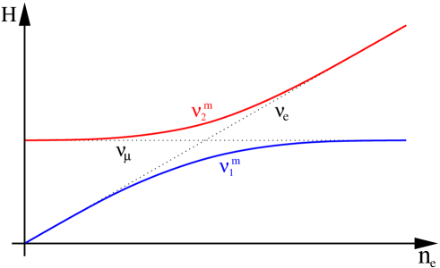
Figure 2.3: Level crossing scheme in two flavors. Shown are the neutrino energy levels in matter as a function of the electron number density $N_{e}$. Dashed line in absence of mixing, solid line with mixing.

In Fig. 2.3 we represent the diagram known as level crossing scheme. It shows the energy levels of $\nu^{m}_{1}$ and $\nu^{m}_{2}$ along with those in absence of mixing (i.e. $\nu_{e}$ and $\nu_{\mu}$) as the function of the electron number density, $N_{e}$. In absence of mixing the energy levels cross at the resonance point, but with non-vanishing mixing the levels repel each other and the avoided level crossing results.
B) Non-adiabatic case
The situation is different when the off-diagonal terms of Eq. (2.55) are comparable or larger than the diagonal ones, $|\dot{\theta}_{m}|\gtrsim|E^{m}_{1}-E^{m}_{2}|$. The adiabatic approximation does not apply anymore, and one has to take into account possible transition between matter eigenstates driven by the violation of the adiabaticity. We can generalize Eq. (2.67) to include this effect in the following way (omitting the oscillatory terms which average to zero),

$$\overline{P(\nu_{e}\to\nu_{\mu})}\simeq\frac{1}{2}-\frac{1}{2}\cos 2\theta^{i}_{m}\cos 2\theta^{f}_{m}(1-2P^{\prime})\,,$$ (2.69)

where $P^{\prime}$ stands for the hopping probability and for small values of the mixing angle is given by the Landau-Zener formula

$$P^{\prime}\simeq e^{-\frac{\pi}{2}\gamma_{\rm res}}\,,$$ (2.70)

where $\gamma_{\rm res}$ is the adiabaticity parameter computed at the resonance point. As discussed in Ref. [63], this expression is valid as long as the density profile can be approximated as linear around the resonance point and the mixing angle is small. For an arbitrary density distribution and mixing angle the general expression is

$$P_{f}=\frac{{\rm exp}(-\frac{\pi}{2}\gamma F)-{\rm exp}(-\frac{\pi}{2}\gamma F/\sin^{2}\theta)}{1-{\rm exp}(-\frac{\pi}{2}\gamma F/\sin^{2}\theta)}~{}~{},$$ (2.71)

where $F$ depends on the density profile and the mixing angle. This expression has to be computed at the resonance point. There are other more general formalisms where the analysis is independent of the resonance and the adiabaticity parameter can be calculated at an arbitrary point [64]. Another useful expression for the jumping probability, which applies for an arbitrary mixing angle, is

$$P^{\prime}\simeq\frac{{\rm exp}(-2\pi L^{-1}_{\rho}\frac{\Delta m^{2}}{2E}\cos^{2}\theta)-1}{{\rm exp}(-2\pi L^{-1}_{\rho}\frac{\Delta m^{2}}{2E})-1}\,,$$ (2.72)

where $L_{\rho}$ is defined in Eq. (2.62). The whole expression can be easily reinterpreted in terms of $\gamma_{\rm res}$.

In the adiabatic limit $\gamma_{\rm res}\gg 1$ and $P^{\prime}\simeq 0$, reproducing Eq. (2.67). In the non-adiabatic limit $\gamma_{\rm res}\ll 1$, and as discussed in Ref. [65] the jumping probability is given by $P^{\prime}\simeq\sin^{2}(\theta_{m}-\theta_{m}^{i})$, where $\theta_{m}^{i}$ is the effective mixing angle at the neutrino production point. If we assume the matter density at that point to be far above the resonance density, we obtain in the limit of $\theta_{m}\to\theta_{0}$ a crossing probability for neutrinos of $P^{\prime}\simeq\cos^{2}\theta_{0}$, which in the case of a small mixing angle reduces to $P^{\prime}\simeq 1$. This situation leads to an interchange between the survival and transition probabilities. If we consider then the case of a very small vacuum mixing angle and $N_{e}^{f}\ll N_{e}^{\rm res}\ll N_{e}^{i}$ (or $N_{e}^{i}\ll N_{e}^{\rm res}\ll N_{e}^{f}$), Eq. (2.69) becomes the simple expression

$$\overline{P(\nu_{e}\to\nu_{\mu})}\simeq 1-P^{\prime}\,,$$ (2.73)

with $P^{\prime}$ given by Eq. (2.72).

2.3 Neutrino oscillations in the SN envelope

After having discussed the generalities of neutrino oscillation physics, we are going to study the actual three flavor situation in the particular case of SN neutrinos. The evolution of neutrinos inside the SN can be divided in two zones: inside the core, dominated by neutrino collisions with matter, and through the envelope, where neutrinos participate only in elastic forward scattering, the border being defined as the neutrino sphere. In this thesis we do not consider what happens inside the core, and parameterize its effect as distribution functions for the neutrinos. We take this distribution functions as input and study their evolution outside the neutrino sphere, as discussed in Chapter 1.

2.3.1 Supernova matter profiles

The main conclusion of the previous sections is that in order to determine the evolution of neutrinos in a medium with varying density we need to know both the neutrino parameters and the properties of the medium, especially the matter and chemical profiles. In a SN scenario, these exhibit an important time dependence during the explosion. Figure 2.4 shows the density $\rho(t,r)$ and the electron fraction $Y_{e}(t,r)$ profiles for a typical SN progenitor as well as at different times post-bounce.

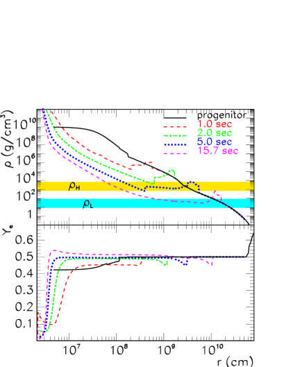
Figure 2.4: Density (upper panel) and electron fraction (bottom panel) profiles for the SN progenitor and at different instants after the core bounce, from Ref. [66]. The regions where the $H$- (yellow) and the $L$- (cyan) resonance take place are also indicated.

The density in the envelope of a SN depends on the characteristics of the progenitor star (mass, metallicity, $\dots$). However, it can be reasonably well approximated by a power law of the type:

$$\rho(r)=\rho_{0}\left(\frac{r_{0}}{r}\right)^{n}~{},$$ (2.74)

where $\rho_{0}\sim 10^{4}$ g/cm³, $r_{0}\sim 10^{9}$ cm, and $n\sim 3$. In Fig. 2.5 we can see how well several profiles adjust to this expression of the density. The electron fraction profile varies depending on the matter composition of the different layers. For instance, typical values of $Y_{e}$ between 0.42 and 0.45 in the inner regions are found in stellar evolution simulations [67]. In the intermediate regions, where the MSW $H$- and $L$-resonances take place $Y_{e}\approx 0.5$. This value can further increase in the most outer layers of the SN envelope due to the presence of hydrogen.

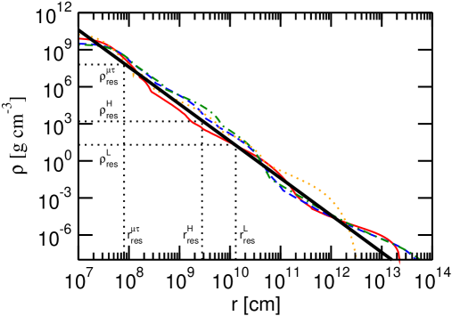
Figure 2.5: Matter density profiles for three different SN progenitor masses: 11 (red solid), 20 (blue dashed) and 30 (green dot-dashed) $M_{\odot}$ from Woosley [68], one from Nomoto [69] for the progenitor of SN1987A (orange dotted) and the expression $\rho=4\times 10^{4}{\rm gcm^{-3}}(10^{9}{\rm cm}/r)^{3}$ (black thick solid line). The regions around the points where the $\mu\tau$, $H$ and $L$-resonances take place are also shown with dotted lines, $r_{\rm res}^{\mu\tau}$, $r_{\rm res}^{H}$ and $r_{\rm res}^{L}$.

After the SN core bounce the matter profile is affected in several ways. First note that a front shock wave starts to propagate outwards and eventually ejects the SN envelope. The evolution of the shock wave will strongly modify the density profile and therefore the neutrino propagation [70, 71]. Following Ref. [66] we have represented in Fig. 2.4 a more complicated structure of the shock wave, where an additional “reverse wave” appears due to the collision of the neutrino-driven wind and the slowly moving material behind the forward shock.

On the other hand, the electron fraction is also affected by the time evolution as the SN explosion proceeds. Let us discuss how it changes during the different stages of the explosion. Once the collapse starts the core density grows so that the neutrinos become eventually effectively trapped within the neutrino sphere. At this point the trapped electron fraction has decreased until values of the order of 0.33 [72]. When the inner core reaches nuclear density it can not contract any further and bounces. As a consequence a shock wave forms in the inner core and starts propagating outwards. When the newly formed SN shock reaches densities low enough for the initially trapped neutrinos to begin streaming faster than the shock propagates [73], a breakout pulse of $\nu_{e}$ is launched. In the shock-heated matter, which is still rich of electrons and completely disintegrated into free neutrons and protons, a large number of $\nu_{e}$ are rapidly produced by electron captures on protons. They follow the shock on its way out until they are released in a very luminous flash, the breakout burst, at about the moment when the shock penetrates the neutrino sphere and the neutrinos can escape essentially unhindered. As a consequence, the lepton number in the layer around the neutrino sphere decreases strongly and the matter neutronizes. The value of $Y_{e}$ steadily decreases in these layers until values of the order of $\mathcal{O}(10^{-2})$. Outside the neutrino sphere there is a steep rise until $Y_{e}\approx 0.5$. This is a robust feature of the neutrino-driven baryonic wind. Neutrino heating drives the wind mass loss and causes $Y_{e}$ to rise within a few $10$ km from low to high values, between 0.45 and 0.55 [74], see bottom panel of Fig. 2.4. Inspired in the numerical results of Ref. [66] we can parameterized the behavior of the electron fraction near the neutrino sphere phenomenologically as,

$$Y_{e}=a+b\arctan[(r-r_{0})/r_{s}]~{},$$ (2.75)

where $a\approx 0.23$–$0.26$ and $b\approx 0.16$–$0.20$. The parameters $r_{0}$ and $r_{s}$ describe where the rise takes place and how steep it is, respectively. As can be seen in Fig. 2.4 both decrease with time.

2.3.2 Factorization of the evolution

In the SN there exists such extreme conditions that neutrinos travel from regions with densities of the order $10^{12}$ g/cm³, right behind the neutrino sphere, to basically zero density at the atmosphere of the star. As a consequence, contrary to the case of the Sun, neutrinos will undergo three kinematic resonant conversions. Two of them come from $V_{\rm CC}$, the $H$-resonance taking place at high densities and defined by $V_{\rm CC}(r^{H}_{\rm res})=\Delta m^{2}_{\rm 31}/(2E)\cos 2\theta_{13}$, and the $L$-resonance occurring at low densities where $V_{\rm CC}(r^{L}_{\rm res})=\Delta m^{2}_{21}/(2E)\cos 2\theta_{12}$. The third one is due to $V_{\mu\tau}$, and is determined by $V_{\mu\tau}(r^{\mu\tau}_{\rm res})=\Delta m^{2}_{31}/(2E)\cos 2\theta_{23}$. These three conditions are represented in the density profiles of Fig. 2.5 and the level crossing diagrams for the three flavor scenario shown in Fig. 2.6. Since the sign of $\Delta m^{2}_{31}$ is undetermined both hierarchies are still possible. The left panel of this figure corresponds to normal hierarchy ($\Delta m^{2}_{31}>0$), which after Eq. (2.52) translates in the $H$-resonance occurring for neutrinos, while the right panel is done for the inverted hierarchy case ($\Delta m^{2}_{31}<0$) and the resonance takes place in the antineutrino channel. The $\mu\tau$-resonance depends not only on the hierarchy, but also on the octant of $\theta_{23}$ as shown in Fig. 2.6.

The interesting point here is that the large difference between the two mass splittings ($\Delta m_{21}^{2}/\Delta m_{31}^{2}\sim 10^{-2}$), and therefore the densities at the resonance layers, allows us to factorize the evolution of neutrinos. We can then treat the three possible transitions as an approximate two neutrino problem. In the $H$-resonance region the mixing $U^{m}_{e2}$ associated to $\Delta m^{2}_{21}$ is suppressed by matter by more than two orders of magnitude,

$$\frac{U_{e2}^{m}}{U_{e2}}\sim\frac{\rho_{L}}{\rho_{H}}\lesssim 10^{-2}~{}.$$ (2.76)

The situation is similar at the $L$-resonance region, where the effects of $\Delta m^{2}_{31}$ basically go as the mixing at vacuum,

$$U_{e3}^{m}=U_{e3}[1+{\cal O}(\xi)]~{},~{}~{}~{}~{}~{}~{}~{}\xi\approx\frac{\rho_{L}}{\rho_{H}}\lesssim 10^{-2}~{}.$$ (2.77)

Finally, the same argument stands for the $\mu\tau$-resonance, where the mixing between $\nu_{\mu}$ or $\nu_{\tau}$ with the third state is suppressed at the resonance by the huge hierarchy between $V_{\mu\tau}$ and $V_{\rm CC}$, ${\cal O}(10^{-4})$.

This means that by an appropriate redefinition of the states we can always disentangle one of the neutrinos, reducing the three neutrino problem to an effective two neutrino one.

2.3.3 Level crossing schemes

As discussed in Sec. 2.2.2, the evolution of neutrinos can be described using the equation of Schrödinger, Eq. (2.41). Far enough from the neutrino sphere, so that no effect is to be expected from neutrino-neutrino interactions, the Hamiltonian involved in the flavor basis is given by

$$H=H_{\rm kin}+H_{\rm int}=\frac{1}{2E}\left(\begin{array}[]{lcc}m_{ee}^{2}+2EV_{\rm CC}&m_{e\mu}^{2}&m_{e\tau}^{2}\\ m_{e\mu}^{2}&m_{\mu\mu}^{2}&m_{\mu\tau}^{2}\\ m_{e\tau}^{2}&m_{\mu\tau}^{2}&m_{\tau\tau}^{2}+2EV_{\mu\tau}\end{array}\right)~{},$$ (2.78)

where the $m^{2}_{\alpha\beta}$ come from the kinetic term,

$$H_{\rm kin}=U\frac{1}{2E}\left(\begin{array}[]{ccc}m_{1}^{2}&0&0\\ 0&m_{2}^{2}&0\\ 0&0&m_{3}^{2}\end{array}\right)U^{\dagger}~{},$$ (2.79)

with $U$ given in Eq. (2.16), and $H_{\rm int}={\rm diag}(V_{\rm CC},0,V_{\mu\tau})$ is the resulting interaction Hamiltonian after removing the NC common terms. By using Eq. (2.78) it is easy to reproduce the level crossing schemes of Fig. 2.6. Its diagonal terms basically determine the energies of the flavor states, represented by dotted lines, while its eigenvalues, represented by the colored solid lines, give the actual neutrino path.

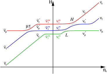
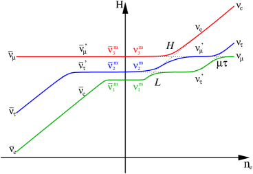
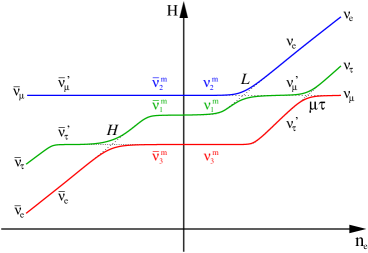
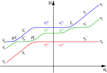
Figure 2.6: Level crossing diagrams for normal (top panels) and inverted mass hierarchy (bottom panels). The left panels correspond to $\theta_{23}<\pi/4$ (first octant) and the right ones to $\theta_{23}>\pi/4$ (second octant). Solid lines show the eigenvalues of the effective Hamiltonian as a function of the electron number density. Dashed lines correspond to energies of the flavor levels $\nu_{e}$, $\nu^{\prime}_{\mu}$ and $\nu^{\prime}_{\tau}$. The part of the plot with $n_{e}<0$ corresponds to the antineutrino channel.

For very high densities, where $V_{\mu\tau}$ and obviously $V_{\rm CC}$ are larger than the kinetic terms, the whole Hamiltonian leading the evolution of neutrinos can be effectively reduced to the interaction one,

$$H\approx\left(\begin{array}[]{lcc}V_{\rm CC}&0&0\\ 0&m_{\mu\mu}^{2}&0\\ 0&0&V_{\mu\tau}\end{array}\right)~{}.$$ (2.80)

As a consequence, the matter and flavor eigenstate coincide, and the eigenvalues will go as shown in the high density region of Fig. 2.6: $\nu_{e}\sim V_{\rm CC}$, $\nu_{\tau}\sim V_{\mu\tau}$ and $\nu_{\mu}\sim m_{\mu\mu}^{2}$, and the same with opposite sign in the potentials for antineutrinos. The $V_{\mu\tau}$ potential will be important if

$$V_{\mu\tau}\gtrsim\Delta m^{2}_{31}/2E\approx 2m_{\mu\tau}^{2}/2E\rightarrow\rho_{\mu\tau}\gtrsim 10^{7}-10^{8}~{}\mbox{g/cm}^{3}.$$ (2.81)

In the interval of densities where $V_{\mu\tau}\ll\Delta m^{2}_{31}/2E\ll V_{\rm CC}$, the $V_{\mu\tau}$ potential can be neglected so that we obtain the Hamiltonian

$$H=\frac{1}{2E}\left(\begin{array}[]{lcc}m_{ee}^{2}+2EV_{\rm CC}&m_{e\mu}^{2}&m_{e\tau}^{2}\\ m_{e\mu}^{2}&m_{\mu\mu}^{2}&m_{\mu\tau}^{2}\\ m_{e\tau}^{2}&m_{\mu\tau}^{2}&m_{\tau\tau}^{2}\end{array}\right)~{}.$$ (2.82)

Now, by diagonalizing the 23-sector,

$$H=\frac{1}{2E}\left(\begin{array}[]{lcc}m_{ee}^{2}+2EV_{\rm CC}&m_{e\mu^{\prime}}^{2}&m_{e\tau^{\prime}}^{2}\\ m_{e\mu^{\prime}}^{2}&m_{\mu^{\prime}\mu^{\prime}}^{2}&0\\ m_{e\tau^{\prime}}^{2}&0&m_{\tau^{\prime}\tau^{\prime}}^{2}\end{array}\right)~{},$$ (2.83)

we will be basically diagonalizing the whole Hamiltonian, since $V_{\rm CC}\gg\Delta m^{2}_{31}/2E$. For this density range $H\approx{\rm diag}(V_{\rm CC},m_{\mu^{\prime}\mu^{\prime}}^{2},m_{\tau^{\prime}\tau^{\prime}}^{2})$, and the resulting matter basis is ($\nu_{e},\nu_{\mu^{\prime}},\nu_{\tau^{\prime}}$). Therefore, in the region $V_{\mu\tau}\sim\Delta m^{2}_{31}/2E$ the level crossing occurs, taking place for neutrinos or antineutrinos depending on the hierarchy and the octant of $\theta_{23}$, as shown in Fig. 2.6. For instance, for normal hierarchy and first octant (top left panel of Fig. 2.6) neutrinos have undergone the transitions $\bar{\nu}_{\mu}\rightarrow\bar{\nu}_{\tau}^{\prime}$, $\bar{\nu}_{\tau}\rightarrow\bar{\nu}_{\mu}^{\prime}$, $\nu_{\mu}\rightarrow\nu_{\mu}^{\prime}$ and $\nu_{\tau}\rightarrow\nu_{\tau}^{\prime}$.

As the density decreases, the potential reaches the different mass scales, producing the level crossings at the resonances. The sign of $\Delta m^{2}_{21}$ is known to be positive, and therefore the $L$-resonance will always take place for neutrinos, but depending on the hierarchy in the neutrino mass scheme, the $H$-resonance will occur for neutrinos (normal hierarchy, $\Delta m^{2}_{31}>0$) or antineutrinos (inverted hierarchy, $\Delta m^{2}_{31}<0$), as shown in Fig. 2.6. The positive values of the density (x-axis) in the level crossings represent the evolution of neutrinos, while that of antineutrinos is shown in the negative $N_{e}$ values. This is a simple trick, that allows us to represent the level crossing schemes in a more compact form, and is motivated by the fact that the effective potential for antineutrinos has the opposite sign than the one for neutrinos. Thus, antineutrinos can be visualized as neutrinos travelling through matter with effectively negative $N_{e}$. Neutrinos will start their evolution from the far right side of the figure, while antineutrinos will be born at the far left side. Both will thereafter evolve towards vacuum, represented as $N_{e}=0$ at the center.

The evolution of neutrinos in the SN envelope will be determined at the resonances, the points where the flavor transitions can occur. Let us then analyze what happens at the different resonances.

2.3.4 Mu-tau-resonance

The crossing of $\nu_{\mu}$ and $\nu_{\tau}$ levels, the $\mu\tau$-resonance, is a consequence of the potential that arises at one loop level due to the difference in the masses of the $\mu$ and $\tau$ leptons [61]. Although $V_{\mu\tau}$ is almost five orders of magnitude smaller than $V_{\rm CC}$, the huge densities in the inner layers of the SN may make it important.

In principle, one could think that this possible crossing does not really matter, since the initial $\nu_{\mu}$ and $\nu_{\tau}$ fluxes are expected to be identical, and therefore no potential effect between them would lead to any observable features. However, the situation changes when we include neutrino-neutrino interactions into the picture. As we will discuss in Chapter 5, these could lead to a transition right before the $\mu\tau$-resonance moving the flux difference to the $\nu_{\mu}$ and $\nu_{\tau}$ branches. It will be then important to understand what happens at the resonance.

The conversion due to the $V_{\mu\tau}$ potential will take place in the dense inner regions, where $\nu_{e}$ is completely decoupled, since $V_{\rm CC}$ is much larger than the elements $H_{1i}$ (i=2,3) in the Hamiltonian of Eq. (2.78). Consequently, we obtain an effective two neutrino problem. The $\mu\tau$-resonance is governed by the atmospheric mixing angle and mass splitting, and the resonance condition is given by

$$V_{\mu\tau}\simeq\frac{\Delta m^{2}_{31}}{2E}\cos 2\theta_{23}\,.$$ (2.84)

Thus, it will take place in the neutrino or antineutrino channel depending on both the hierarchy scheme and the octant of $\theta_{23}$, due to the combination of signs of $\Delta m^{2}_{31}$, $\cos 2\theta_{23}$ and $V_{\mu\tau}$. Numerically, one gets $\rho_{\mu\tau}\gtrsim 10^{7}-10^{8}~{}\mbox{g/cm}^{3}$. Applying Eq. (2.72) at the resonance point, it can be obtained [75]

$$P^{\prime}_{\mu\tau}=\frac{e^{\chi\cos^{2}\theta_{23}}-1}{e^{\chi}-1}\,,$$ (2.85)

$$\chi\equiv-2\pi\frac{\Delta m^{2}_{31}}{2E}\left|\frac{1}{V_{\mu\tau}}\frac{{\rm d}V_{\mu\tau}}{{\rm d}r}\right|^{-1}_{res}\,.$$ (2.86)

Substituting into this expression the potential profile and parameters, we find $\chi\approx 500$–$900$, which corresponds to a very good adiabaticity: $P^{\prime}_{\mu\tau}=0$.

2.3.5 H-resonance

Let us move now to the resonances due to the $V_{\rm CC}$, and let us start with the high density one, $H$-resonance. In order to reduce the three-neutrino problem to a two-neutrino one we should diagonalize the submatrix ($\nu_{\mu},\nu_{\tau}$). However, this transformation leads to very complicated expressions for the Hamiltonian and no easy analytical formulae can be derived. As an approach to the problem, though, we can undo the rotation $V_{23}$ of Eq. (2.16) which to a good approximation diagonalizes the desired submatrix [76]. After performing such rotation the Hamiltonian takes the following form:

$$H^{H} = V^{\dagger}_{23}(UH_{\rm kin}U^{\dagger}+H_{\rm int})V_{23}=$$ (2.90)

$$= \left(\begin{array}[]{ccc}\Delta_{\rm atm}s^{2}_{13}-\Delta_{\odot}c^{2}_{13}c^{2}_{12}+V_{\rm CC}&\frac{1}{2}\Delta_{\odot}c_{13}s2_{12}&\frac{1}{2}\left(\Delta_{\rm atm}s2_{13}+\Delta_{\odot}c^{2}_{12}s2_{13}\right)\\ \frac{1}{2}\Delta_{\odot}c_{13}s2_{12}&-\Delta_{\odot}s^{2}_{12}&-\frac{1}{2}\Delta_{\odot}s2_{12}s_{13}\\ \frac{1}{2}\left(\Delta_{\rm atm}s2_{13}+\Delta_{\odot}c^{2}_{12}s2_{13}\right)&-\frac{1}{2}\Delta_{\odot}s2_{12}s_{13}&\Delta_{\rm atm}c^{2}_{13}-\Delta_{\odot}c^{2}_{12}s^{2}_{13}\end{array}\right)~{},$$

where $\Delta_{\rm atm}\equiv(m^{2}_{3}-m^{2}_{1})/2E$, $\Delta_{\odot}\equiv(m^{2}_{2}-m^{2}_{1})/2E$, $s2_{ij}\equiv\sin{2\theta_{ij}}$, $c2_{ij}\equiv\cos{2\theta_{ij}}$, $s^{2}_{ij}\equiv\sin^{2}{\theta_{ij}}$ and $c^{2}_{ij}\equiv\cos^{2}{\theta_{ij}}$. In the approximation where $\Delta_{\odot}\ll\Delta_{\rm atm}$ this Hamiltonian reduces to the one given in Eq. (2.83) and the evolution of neutrinos breaks to a decoupled one ($\nu^{\prime}_{\mu}$) and a two-neutrino mass matrix of the type of Eq. (2.45).

The resonance point will be now obtained using the condition $H^{H}_{33}-H^{H}_{11}=0$, which gives $V_{\rm CC}=(\Delta_{\rm atm}+\Delta_{\odot}c^{2}_{12})c2_{13}$. Applying Eq. (2.38) we find that the density at the resonance point is given by

$$\rho_{H}=\frac{(\Delta_{\rm atm}+\Delta_{\odot}c^{2}_{12})c2_{13}}{V_{0}Y_{e}}~{}.$$ (2.92)

Assuming that $Y_{e}\simeq 0.5$ around these layers of the SN, we find the density range for the resonance region $5\times 10^{4}$ g/cm${}^{3}\gtrsim\rho_{H}\gtrsim 10^{3}$ g/cm³ for the typical energy range of the SN neutrinos, 1 MeV $\lesssim E\lesssim$ 50 MeV.

We can now calculate the adiabaticity parameter at the resonance using Eq. (2.58). Taking into account that $H^{H}_{33}-H^{H}_{11}=0$, we obtain:

$$\gamma^{-1}_{H}=\left|\frac{\dot{V}_{\rm CC}}{(\Delta_{\rm atm}s2_{13}+\Delta_{\odot}c^{2}_{12}s2_{13})^{2}}\right|_{\rm res}~{}.$$ (2.93)

Making use of Eqs. (2.38), (2.74) and (2.92) we can reexpress the adiabaticity parameter at the $H$-resonance as

$$\gamma^{-1}_{H}=\left|\frac{-5.9\times 10^{-5}(c2_{13})^{4/3}}{\left((\Delta_{\rm atm}+\Delta_{\odot}c^{2}_{12})^{2}V_{0}Y_{e}\rho_{0}\right)^{1/3}(s2_{13})^{2}r_{0}}\right|~{},$$ (2.94)

where $\Delta_{\rm atm}$ and $\Delta_{\odot}$ are given in eV, $\rho_{0}$ in g/cm³ and $r_{0}$ in cm.

In Fig. 2.7 we show the corresponding jumping probability contours for the whole $\Delta m^{2}-\sin^{2}2\theta$ space of parameters. To the right of the dashed blue line we obtain an adiabatic evolution, while to the left of the solid red line the evolution is highly non-adiabatic. The gray band shows the allowed region for the parameters involved in the $H$-resonance at 3$\sigma$, as given in Table 2.1. The dotted vertical lines in the figure mark the adiabaticity borders for this case. In the figure we see, and can be calculated from Eq. (2.94), that for $\sin^{2}\theta_{13}\gtrsim 10^{-3}$ the evolution is adiabatic, while $\sin^{2}\theta_{13}\lesssim 10^{-5}$ leads to a non-adiabatic evolution.

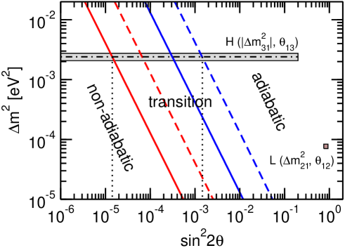
Figure 2.7: Contours of constant hopping probability $P^{\prime}$. The solid lines correspond to a neutrino energy of $E=5$ MeV, the left one (red) stands for $P^{\prime}=0.9$ (highly non-adiabatic transition) and the right one (blue) to $P^{\prime}=0.1$ (adiabatic transition). The dashed lines are done for neutrinos with $E=50$ MeV. The gray band shows the current allowed region at 3$\sigma$ for the parameters involved in the $H$-resonance, for which the vertical lines mark the borders for adiabatic and non-adiabatic conversions. The small brown band shows the current allowed region for the $L$-parameters, lying in the adiabatic region.

2.3.6 L-resonance

In order to properly study the adiabaticity at the $L$-resonance, we undo the rotations $V_{23}$ and $W_{13}$ in the flavor basis around the resonance point [76]. The corresponding Hamiltonian is given by

$$H^{L} = W^{\dagger}_{13}V^{\dagger}_{23}(UH_{\rm kin}U^{\dagger}+H_{\rm std})V_{23}W_{13}=$$ (2.98)

$$= \left(\begin{array}[]{ccc}-\Delta_{\odot}c^{2}_{12}+V_{\rm CC}c^{2}_{13}&\frac{1}{2}\Delta_{\odot}s2_{12}&V_{\rm CC}s2_{13}\\ \frac{1}{2}\Delta_{\odot}s2_{12}&-\Delta_{\odot}s^{2}_{12}&0\\ V_{\rm CC}s2_{13}&0&\Delta_{\rm atm}+V_{\rm CC}s^{2}_{13}\end{array}\right)~{}.$$

From this equation it is easy to see that the third neutrino decouples ($\Delta_{\rm atm}\gg V_{\rm CC}s2_{13}$, for the lower resonance), leaving us with the effective two-neutrino evolution governed by the 1-2 submatrix in $H^{L}$.

The resonance point will be given by $H^{L}_{22}-H^{L}_{11}=0$, thus $V_{\rm CC}c^{2}_{13}=\Delta_{\odot}c2_{12}$. Just as before, we can obtain the density at the resonance point

$$\rho_{L}=\frac{\Delta_{\odot}c2_{12}}{V_{0}Y_{e}c^{2}_{13}}~{},$$ (2.99)

and what we were looking for, the adiabaticity parameter,

$$\gamma^{-1}_{L}=\left|\frac{\dot{V}_{\rm CC}c^{2}_{13}}{(\Delta_{\odot}s2_{12})^{2}}\right|_{\rm res}~{}.$$ (2.100)

Again, making use of Eqs. (2.38), (2.74) and (2.99) we can reexpress the adiabaticity parameter at the $L$-resonance as

$$\gamma^{-1}_{L}=\left|\frac{-5.9\times 10^{-5}(c2_{12})^{4/3}}{\left((\Delta_{\odot}^{2}V_{0}Y_{e}\rho_{0}\right)^{1/3}(s2_{12})^{2}r_{0}}\right|~{}.$$ (2.101)

We can see how the adiabaticity parameter at the $L$-resonance has essentially the same expression as the one at the $H$-resonance, Eq. (2.94), but changing $\Delta_{\rm atm}\to\Delta_{\odot}$ and $\theta_{13}\to\theta_{12}$, provided that $\Delta_{\odot}/\Delta_{\rm atm}\ll 1$ and $\sin^{2}\theta_{13}\ll 1$. This allows us to use the same contours of constant jumping probability of Fig. 2.7, if we reinterpret the oscillation parameters as $\Delta m^{2}_{21}$ and $\sin^{2}2\theta_{12}$. The small brown band in the figure shows the current allowed region at 3$\sigma$ for these parameters given in Table 2.1. Since both neutrino properties are rather well constrained, we can conclude that the $L$-resonance is always adiabatic, and takes place in the neutrino channel.

Chapter 3 Non-Standard Neutrino Interactions

3.1 Introduction

The confirmation of the neutrino oscillation interpretation of solar and atmospheric neutrino data by reactor [77] and accelerator [78, 4] neutrino experiments provides a unique picture of neutrino physics in terms of three-neutrino oscillations [6], leaving little room for other non-standard neutrino properties [79]. Nevertheless, it has long been recognized that any gauge theory of neutrino mass generation inevitably introduces dimension-6 non-standard neutrino interaction (NSI) terms. Such sub-weak strength operators arise in the broad class of seesaw-type models, due to the non-trivial structure of charged and neutral current weak interactions [80], and may be sizeable [81, 82, 83, 84, 85]. Alternatively, neutrino NSI may arise in models where neutrino masses are radiatively “calculable” [86, 87]. Finally, in some supersymmetric unified models, the strength of neutrino NSI may arise from renormalization and/or threshold effects [88].

We stress that NSI strengths are highly model dependent. In some models NSI strengths are too small to be relevant for neutrino propagation, because they are either suppressed by some large mass scale or restricted by limits on neutrino masses, or both. However, this need not be the case, and there are many theoretically attractive scenarios where moderately large NSI strengths are possible and consistent with the smallness of neutrino masses. In fact one can show that NSI may exist even in the limit of massless neutrinos [81, 82, 83, 84, 85]. This may also occur in the context of fully unified models like $SO(10)$ [89].

We argue that, in addition to the precision determination of the oscillation parameters, it is necessary to test for sub-leading non-oscillation effects that could arise from neutrino NSI. These are natural outcome of many neutrino mass models and can be of two types: flavor-changing (FC) and non-universal (NU). These are constrained by existing experiments (see Sec. 3.3) and, with neutrino experiments now entering a precision phase [5], an improved determination of neutrino parameters and their theoretical impact constitute an important goal in astroparticle and high energy physics [6].

One of the objectives of this thesis is the study of neutrino NSI, since they would open a new window to physics beyond the Standard Model. We have performed several analysis in the subject using neutrinos from different scenarios. In this chapter, after introducing the NSI parameterization and summarizing the current limits on the parameters, we will discuss what we can learn about the possible NSI using the combination of MINOS and OPERA, two experiments currently taking data. In Chapter 6 we will present the possibility of probing these NSI using SN neutrinos.

3.2 Parameterization

A large class of NSI may be parameterized with the effective low-energy four-fermion operator:

$$\mathcal{L}_{\rm nsi}=-\varepsilon^{fP}_{\alpha\beta}2\sqrt{2}G_{F}(\bar{\nu}_{\alpha}\gamma_{\mu}L\nu_{\beta})(\bar{f}\gamma^{\mu}Pf)~{}.$$ (3.1)

where $P=L$ or $R$ and $f$ is a first generation fermion: $e,~{}u,~{}d$. The coefficients $\varepsilon^{fP}_{\alpha\beta}$ denote the strength of the NSI between the neutrinos of flavors $\alpha$ and $\beta$ and the $P$-handed component of the fermion $f$. This Lagrangian describes the elastic scattering processes

$$\nu_{\alpha}~{}f\to\nu_{\beta}~{}f~{}~{}~{}~{}\alpha,\beta=e,\mu,\tau~{},$$ (3.2)

schematically represented in Fig. 3.1.

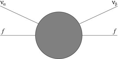
Figure 3.1: Schematic diagram of the neutrino NSI described by the effective low-energy four-fermion operator given in Eq. (3.1).

Just as in the SM case, we can calculate the potential induced in the evolution of neutrinos due to this new interactions. We can rewrite Eq. (3.1) as

$$\mathcal{L}_{\rm nsi} = \frac{1}{\sqrt{2}}G_{F}\{\bar{\nu}_{\alpha}\gamma^{\mu}(1-\gamma_{5})\nu_{\beta}\}\left(\varepsilon^{fL}_{\alpha\beta}\{\bar{f}\gamma_{\mu}(1-\gamma_{5})f\}+\varepsilon^{fR}_{\alpha\beta}\{\bar{f}\gamma_{\mu}(1+\gamma_{5})f\}\right)=$$ (3.3)

$$= \frac{1}{\sqrt{2}}G_{F}\{\bar{\nu}_{\alpha}\gamma^{\mu}(1-\gamma_{5})\nu_{\beta}\}\left\{\bar{f}\gamma_{\mu}\left[(\varepsilon^{fL}_{\alpha\beta}+\varepsilon^{fR}_{\alpha\beta})-(\varepsilon^{fL}_{\alpha\beta}-\varepsilon^{fR}_{\alpha\beta})\gamma_{5}\right]f\right\}~{}.$$

The effective axial vector coupling, $(\varepsilon^{fL}_{\alpha\beta}-\varepsilon^{fR}_{\alpha\beta})$, does not contribute to the coherent elastic scattering of neutrinos with the particles in an unpolarized medium, as we discussed in the calculation of $V_{\rm CC}$ and $V_{\rm NC}$. The vector coupling, $\varepsilon^{fV}_{\alpha\beta}\equiv(\varepsilon^{fL}_{\alpha\beta}+\varepsilon^{fR}_{\alpha\beta})$, on the other hand does affect neutrino propagation in matter, and although no positive signs of them have yet been obtained there are limits on their magnitude as we will later discuss.

Finally, the presence of NSI like the ones described in the Lagrangian of Eq. (3.1) induces the following potentials on neutrinos:

$$V^{\rm FC}_{\alpha\beta}=\sum_{f}\sqrt{2}G_{F}N_{f}\varepsilon^{fV}_{\alpha\beta}~{}, \alpha\neq\beta~{},$$ (3.4)

$$V^{\rm NU}_{\alpha\alpha}=\sum_{f}\sqrt{2}G_{F}N_{f}\varepsilon^{fV}_{\alpha\alpha}~{},$$ (3.5)

where $V^{\rm FC}_{\alpha\beta}$ correspond to the scattering amplitudes in the flavor changing processes $\nu_{\alpha}~{}f\to\nu_{\beta}~{}f$, while $V^{\rm NU}_{\alpha\alpha}$ represents the difference between the non-standard and the standard components in the elastic scattering amplitudes of $\nu_{\alpha}~{}f\to\nu_{\alpha}~{}f$. In general, we can write:

$$V^{\rm nsi}_{\alpha\beta}=\sum_{f}\sqrt{2}G_{F}N_{f}\varepsilon^{fV}_{\alpha\beta}~{},$$ (3.6)

where in principle we sum over all three fundamental fermions found in ordinary matter. However, due to the complexity of a global analysis, usually the studies are done for each one of them separately. The number density for the different fermions will be given by:

$$N_{f}=\left\{\begin{array}[]{ll}N_{e},&f=e\\ N_{p}+2N_{n},&f=d\\ 2N_{p}+N_{n},&f=u\end{array}\right.$$ (3.7)

If we add this new part to the Hamiltonian discussed in Chapter 2, with its kinetic and standard matter interaction terms, we obtain,

$${H=\frac{1}{2E}U\left(\begin{array}[]{ccc}0&0&0\\ 0&\Delta m^{2}_{21}&0\\ 0&0&\Delta m^{2}_{31}\end{array}\right)U^{\dagger}+\left(\begin{array}[]{ccc}V_{\rm CC}&0&0\\ 0&0&0\\ 0&0&0\end{array}\right)+\left(\begin{array}[]{ccc}V^{\rm nsi}_{ee}&V^{\rm nsi}_{e\mu}&V^{\rm nsi}_{e\tau}\\ V^{\rm nsi*}_{e\mu}&V^{\rm nsi}_{\mu\mu}&V^{\rm nsi}_{\mu\tau}\\ V^{\rm nsi*}_{e\tau}&V^{\rm nsi*}_{\mu\tau}&V^{\rm nsi}_{\tau\tau}\end{array}\right)\,,}$$ (3.8)

where $V^{\rm nsi}_{\alpha\beta}$ are given in Eq. (3.6), and $V^{\rm nsi*}_{\alpha\beta}=V^{\rm nsi*}_{\beta\alpha}$ for Hermiticity of the Hamiltonian.

3.3 Current limits

Current bounds on the NSI parameters can be obtained from different sources: laboratory experiments, solar, reactor, atmospheric and accelerator neutrino experiments, cosmology and SN neutrinos. The latter case will be discussed in detail in Chapter 6, while we will here review the present limits coming from the rest of the experiments. Note that these limits have been obtained by varying each $\varepsilon_{\alpha\beta}$ one at a time. In general, when correlations among different $\varepsilon_{\alpha\beta}$ are included the bounds become weaker.

3.3.1 Laboratory

The measurement of $\nu e$ and $\nu q$ elastic cross sections in neutrino scattering experiments [90, 91, 92, 93, 94] provide the following bounds on the NSI parameters, $|\varepsilon^{fP}_{\mu\mu}|\lesssim 10^{-3}$–$10^{-2},~{}|\varepsilon^{fP}_{ee}|\lesssim 10^{-1}$–$1,~{}|\varepsilon^{fP}_{\mu\tau}|\lesssim 0.1,~{}|\varepsilon^{fP}_{e\tau}|\lesssim 0.5$ at 90 % C.L [95, 96, 97]. On the other hand the analysis of the $e^{+}e^{-}\to\nu\bar{\nu}\gamma$ cross section measured at LEP II leads to a bound on $|\varepsilon^{eP}_{\tau\tau}|\lesssim 0.5$ [98]. Future prospects to improve the current limits imply the measurement of $\sin^{2}\theta_{W}$ leptonically in the scattering off electrons in the target, as well as in neutrino deep inelastic scattering in a future neutrino factory. The main improvement would be in the case of $|\varepsilon^{fP}_{ee}|$ and $|\varepsilon^{fP}_{e\tau}|$, where values as small as $10^{-3}$ and $0.02$, respectively, could be reached [96].

The search for flavor violating processes involving charged leptons is expected to restrict the corresponding neutrino interactions, to the extent that the $SU(2)$ gauge symmetry is assumed. However, this can at most give indicative order-of-magnitude restrictions, since we know $SU(2)$ is not a good symmetry of nature. Using radiative corrections it has been argued that, for example, $\mu$-$e$ conversion on nuclei like in the case of Ti$\mu$ also constrains $|\varepsilon^{qP}_{e\mu}|\lesssim 7.7\times 10^{-4}$ [96]. The rather good bound $|\varepsilon^{eP}_{e\mu}|\lesssim 5\times 10^{-4}$ is also obtained because of the strong experimental limit on $\mu\to 3e$ transitions. Finally, only an $\mathcal{O}(1-10)$ limit can be imposed on $|\varepsilon^{eP}_{\tau\tau}|$ from $\tau$ decays.

A detailed relation of the commented limits is given in Table 3.1 [99].

Table 3.1: Present bounds at 90% CL on the NC-like NSI couplings $\varepsilon_{\alpha\beta}^{fP}$ from non-oscillation experiments. Limits have been obtained by varying each $\varepsilon_{\alpha\beta}$ one at a time, with all the others set to zero. Table taken from [99].

Left-handed	Right-handed	Process	Experiment	Reference
$-0.03<\varepsilon_{ee}^{eL}<0.08$	$0.004<\varepsilon_{ee}^{eR}<0.15$	$\begin{aligned} \nu_{e}e&\to\nu e\\[-5.69054pt] \bar{\nu}_{e}e&\to\bar{\nu}e\end{aligned}$	$\begin{aligned} &\text{LSND}\\[-5.69054pt] &\text{Reactors}\end{aligned}$	[97, 100]
$-1<\varepsilon_{ee}^{uL}<0.3$	$-0.4<\varepsilon_{ee}^{uR}<0.7$	$\nu_{e}q\to\nu q$	CHARM	[96]
$-0.3<\varepsilon_{ee}^{dL}<0.3$	$-0.6<\varepsilon_{ee}^{dR}<0.5$	$\nu_{e}q\to\nu q$	CHARM	[96]
$|\varepsilon_{\mu\mu}^{eL}|<0.03$	$|\varepsilon_{\mu\mu}^{eR}|<0.03$	$\nu_{\mu}e\to\nu e$	CHARM II	[96, 100]
$|\varepsilon_{\mu\mu}^{uL}|<0.003$	$-0.008<\varepsilon_{\mu\mu}^{uR}<0.003$	$\nu_{\mu}q\to\nu q$	NuTeV	[96]
$|\varepsilon_{\mu\mu}^{dL}|<0.003$	$-0.008<\varepsilon_{\mu\mu}^{dR}<0.015$	$\nu_{\mu}q\to\nu q$	NuTeV	[96]
$-0.5<\varepsilon_{\tau\tau}^{eL}<0.2$	$-0.3<\varepsilon_{\tau\tau}^{eR}<0.4$	$e^{+}e^{-}\to\nu\bar{\nu}\gamma$	LEP	[98, 100]
$|\varepsilon_{\tau\tau}^{uL}|<1.4$	$|\varepsilon_{\tau\tau}^{uR}|<3$	rad. corrections	$\tau$ decay	[96]
$|\varepsilon_{\tau\tau}^{dL}|<1.1$	$|\varepsilon_{\tau\tau}^{dR}|<6$	rad. corrections	$\tau$ decay	[96]
$|\varepsilon_{e\mu}^{eL}|<0.0005$	$|\varepsilon_{e\mu}^{eR}|<0.0005$	rad. corrections	$\mu\to 3e$	[96]
$|\varepsilon_{e\mu}^{uL}|<0.0008$	$|\varepsilon_{e\mu}^{uR}|<0.0008$	rad. corrections	$\text{Ti}\,\mu\to\text{Ti}\,e$	[96]
$|\varepsilon_{e\mu}^{dL}|<0.0008$	$|\varepsilon_{e\mu}^{dR}|<0.0008$	rad. corrections	$\text{Ti}\,\mu\to\text{Ti}\,e$	[96]
$|\varepsilon_{e\tau}^{eL}|<0.33$	$|\varepsilon_{e\tau}^{eR}|<0.28$	$\nu_{e}e\to\nu e$	LEP+LSND+Rea	[98, 100]
$|\varepsilon_{e\tau}^{uL}|<0.5$	$|\varepsilon_{e\tau}^{uR}|<0.5$	$\nu_{e}q\to\nu q$	CHARM	[96]
$|\varepsilon_{e\tau}^{dL}|<0.5$	$|\varepsilon_{e\tau}^{dR}|<0.5$	$\nu_{e}q\to\nu q$	CHARM	[96]
$|\varepsilon_{\mu\tau}^{eL}|<0.1$	$|\varepsilon_{\mu\tau}^{eR}|<0.1$	$\nu_{\mu}e\to\nu e$	CHARM II	[96, 100]
$|\varepsilon_{\mu\tau}^{uL}|<0.05$	$|\varepsilon_{\mu\tau}^{uR}|<0.05$	$\nu_{\mu}q\to\nu q$	NuTeV	[96]
$|\varepsilon_{\mu\tau}^{dL}|<0.05$	$|\varepsilon_{\mu\tau}^{dR}|<0.05$	$\nu_{\mu}q\to\nu q$	NuTeV	[96]

3.3.2 Solar and reactor

NSI can also affect neutrino propagation through matter, probed in current neutrino oscillation experiments. The bounds so obtained apply to the vector coupling constant of the NSI, $\varepsilon^{fV}_{\alpha\beta}=\varepsilon^{fL}_{\alpha\beta}+\varepsilon^{fR}_{\alpha\beta}$, since only this combination appears in neutrino propagation in matter, as previously discussed.

The role of neutrino NSIs as subleading effects on the solar neutrino oscillations and KamLAND has been considered in Refs. [101, 102, 103] with the following bounds at 90 % CL for $\varepsilon\equiv-\sin\theta_{23}\varepsilon^{dV}_{e\tau}$ with the allowed range $-0.93\lesssim\varepsilon\lesssim 0.30$, while for the diagonal term $\varepsilon^{\prime}\equiv\sin^{2}\theta_{23}\varepsilon^{dV}_{\tau\tau}-\varepsilon^{dV}_{ee}$, the only forbidden region is $[0.20,0.78]$ [103]. Only in the ideal case of infinitely precise determination of the solar neutrino oscillation parameters, the allowed range would “close from the left” for negative NSI parameter values, at $-0.6$ for $\varepsilon$ and $-0.7$ for $\varepsilon^{\prime}$.

3.3.3 Atmospheric and accelerator neutrinos

NSI involving muon neutrinos can be constrained by atmospheric neutrino experiments as well as accelerator neutrino oscillation searches at K2K and MINOS. In Ref. [104] Super-Kamiokande and MACRO observations of atmospheric neutrinos were considered in the framework of two neutrinos. The limits obtained were $-0.05\lesssim\varepsilon^{dV}_{\mu\tau}<0.04$ and $|\varepsilon^{dV}_{\tau\tau}-\varepsilon^{dV}_{\mu\mu}|\lesssim 0.17$ at 99 % CL. The same data set together with K2K were recently considered in Refs. [105, 106] to study the nonstandard neutrino interactions in a three generation scheme under the assumption $\varepsilon_{e\mu}=\varepsilon_{\mu\mu}=\varepsilon_{\mu\tau}=0$. The most recent analysis including also accelerator experiments [48] gives at 3$\sigma$, $|\varepsilon_{\mu\tau}^{eV}|\leq 0.058\,,|\varepsilon_{\tau\tau}^{eV}-\varepsilon_{\mu\mu}^{eV}|\leq 0.19\,,|\varepsilon_{\mu\tau}^{uV}|\leq 0.019\,,|\varepsilon_{\tau\tau}^{uV}-\varepsilon_{\mu\mu}^{uV}|\leq 0.061\,,|\varepsilon_{\mu\tau}^{dV}|\leq 0.019\,,|\varepsilon_{\tau\tau}^{dV}-\varepsilon_{\mu\mu}^{dV}|\leq 0.060$.

3.3.4 Cosmology

If NSI with electrons were large they might also lead to important cosmological and astrophysical implications. For instance, relic neutrinos could have been kept in thermal contact with electrons and positrons for a longer time than in the standard case, hence they would share a larger fraction of the entropy release from $e^{\pm}$ annihilations. This would affect the predicted features of the cosmic background of neutrinos, in particular, it could enhance the radiation content of the Universe. As pointed out in Ref. [107], the required NSI couplings to observe this kind of effects with cosmological mesurements are larger than the current laboratory bounds.

3.4 Can OPERA help in constraining neutrino non-standard interactions?

The interplay of oscillation and neutrino NSI was studied in [108] and subsequently it was shown [109, 110] that in the presence of NSI it is very difficult to disentangle genuine oscillation effects from those coming from NSI. The latter may affect production, propagation and detection of neutrinos and in general these three effects need not be correlated. It has been shown that in this case cancellations can occur which make it impossible to separate oscillation from NSI effects. Subsequently it was discovered that the ability to detect $\nu_{\tau}$ may be crucial in order to overcome that problem [111], though this method requires sufficiently large beam energies to be applicable. Barring the occurrence of fine-tuned cancellations, NSI and oscillations have very different $L/E$ dependence. Therefore, combining different $L/E$ can be very effective in probing the presence of NSI. The issue of NSI and oscillation in neutrino experiments with terrestrial sources has been studied in a large number of publications [112, 113, 114, 115, 116, 117, 118, 119, 120, 121, 110, 111, 122, 123, 124, 125, 126]. In Ref. [118] it was shown that MINOS [4] on its own is not able to put new constraints on NSI parameters. On the other hand, in Ref. [117] the combination of atmospheric data with MINOS was proven to be effective in probing at least some of the NSI parameters. Since matter effects are relatively small in MINOS, its main role in that combination is to constrain the vacuum mixing parameters.

The question we would like to address here is whether the combination of MINOS and OPERA [127] can provide useful information on NSI. OPERA has recently seen the first events in the emulsion cloud chamber [128] and hence it appears timely to ask this question. The idea is that OPERA will be able to detect $\nu_{\tau}$ and has a very different $L/E$ than MINOS. Both factors are known to help distinguish NSI from oscillation effects. Clearly, much larger improvements on existing sensitivities are expected from superbeam experiments like T2K [129] and NO$\nu$A [130] especially in combination with reactor neutrino experiments like Double Chooz [131, 132] or Daya Bay [133], see Ref. [126]. We will here focus on the simple case where NSI only affects neutrino propagation.

3.4.1 Basic setup

A) Evolution Hamiltonian
The evolution of neutrinos will be governed by the Hamiltonian given in Eq. (6.31)

$${H=\frac{1}{2E}U\left(\begin{array}[]{ccc}0&0&0\\ 0&\Delta m^{2}_{21}&0\\ 0&0&\Delta m^{2}_{31}\end{array}\right)U^{\dagger}+V_{\rm CC}\left(\begin{array}[]{ccc}1&0&0\\ 0&0&0\\ 0&0&0\end{array}\right)+V_{\rm CC}\left(\begin{array}[]{ccc}0&0&\varepsilon_{e\tau}\\ 0&0&0\\ \varepsilon_{e\tau}&0&\varepsilon_{\tau\tau}\end{array}\right)\,,}$$ (3.9)

where we have assumed the $\varepsilon$’s to be real for simplicity. We have also made use of the fact that all $\varepsilon_{x\mu}$ are fairly well constrained and hence are expected not to play a significant role at leading order. The effect of $\varepsilon_{ee}$ is a re-scaling of the matter density and all experiments considered here are not expected to be sensitive to standard matter effects. Hence we will set $\varepsilon_{ee}=0$. Note, that the $\varepsilon$ as defined here, are effective parameters. At the level of the underlying Lagrangian describing the NSI, the NSI coupling of the neutrino can be either to electrons, up or down quarks. From a phenomenological point of view, however, only the (incoherent) sum of all these contributions is relevant. For simplicity, we chose to normalize our NSI to the electron abundance. This introduces a relative factor of 3 compared to the case where one normalizes either to the up or down quark abundance (assuming an isoscalar composition of the Earth), i.e. the NSI coupling to only up or down quark would need to be 3 times as strong to produce the same effect in oscillations. Since both conventions can be found in the literature, care is required in making quantitative comparisons.

There are two potential benefits beyond adding statistics from combining the data from MINOS and OPERA: First, OPERA can detect $\nu_{\tau}$ which, in principle, allows to directly access any effect from $\varepsilon_{x\tau}$. Moreover, although the baseline is the same, the beam energies are very different $\langle E\rangle\simeq 3\,\mathrm{GeV}$ for MINOS, whereas $\langle E\rangle\simeq 17\,\mathrm{GeV}$ for OPERA.
B) Experiments
All numerical simulations have been done using the GLoBES (General Long Baseline Experiment Simulator) software [135, 136], a package especially designed for the simulation of long baseline neutrino oscillation experiments. In order to include the effects of the NSI we have customized the package by adding a new piece to the Hamiltonian as shown in Eq. (3.9). We have considered three different experiments: MINOS, OPERA and Double Chooz, the main characteristics of which are summarized in table 3.2.

Label	$L$	$\langle E_{\nu}\rangle$	Power	$t_{\rm run}$	Channel
MINOS2 (M2)	735 km	3 GeV	$5\times 10^{20}$ pot/yr	5 yr	$\nu_{\mu}\to\nu_{e,\mu}$
OPERA (O)	732 km	17 GeV	$4.5\times 10^{19}$ pot/yr	5 yr	$\nu_{\mu}\to\nu_{e,\mu,\tau}$
Double Chooz (DC)	0.2 km (near)	4 MeV	$8.4$ GW	5 yr	$\bar{\nu}_{e}\to\bar{\nu}_{e}$
	1.05 km (far)

Table 3.2: Main parameters of the experiments under study.

MINOS is a long baseline neutrino oscillation experiment using the NuMI neutrino beam, at FNAL. It uses two magnetized iron calorimeters. One serves as near detector and is located at about $1\,\mathrm{km}$ from the target, whereas the second, larger one is located at the Soudan Underground Laboratory at a distance of $735\,\mathrm{km}$ from the source. The near detector is used to measure the neutrino beam spectrum and composition. The near/far comparison also mitigates the effect of cross section uncertainties and various systematical errors. In our simulations, based on [137, 138, 139], we have used a running time of 5 years with a statistics corresponding to a primary proton beam of $5\times 10^{20}$ per year, giving a total of $2.5\times 10^{21}$, the maximum reachable value reported by the MINOS collaboration. The mean energy of the neutrino beam is $\langle E\rangle\simeq 3\,\mathrm{GeV}$.

The OPERA detector is located at Gran Sasso and gets its beam from CERN (CNGS). OPERA consists of two parts: a muon tracker and an emulsion cloud chamber. The latter one is the part which is able to discern a $\nu_{\tau}$ charged current interaction by identifying the subsequent $\tau$-decay. The baseline is $732\,\mathrm{km}$. Following [137, 127, 140] we assume a 5 year run with a nominal beam intensity of $4.5\times 10^{19}\,\mathrm{pot}$ per year. The CNGS neutrino beam has an average energy of $\langle E\rangle\simeq 17\,\mathrm{GeV}$. Since both MINOS and OPERA have the same baseline we use the same matter density which we take constant and equal to its value at the Earth’s crust, that is $\rho=2.7$ g/cm³.

Finally, Double Chooz is a reactor experiment, to be located in the old site of CHOOZ, in France. The experiment consists of a pair of nearly identical near and far detectors, each with a fiducial mass of $10.16\,\mathrm{t}$ of liquid scintillator. The detectors are located at a distance of $0.2\,\mathrm{km}$ and $1.05\,\mathrm{km}$ respectively. As considered in [141] we assume the thermal power of both reactor cores to be 4.2 GW and a running time of 5 years. The neutrinos mean energy is $\langle E\rangle\simeq 4\,\mathrm{MeV}$.

Concerning the neutrino oscillation parameters used to calculate the simulated event rates, we have taken the best fit values as given in Ref. [45], unless stated otherwise:

$$\begin{array}[]{rclrcl}\sin^{2}\theta^{\rm true}_{12}&=&0.32,&(\Delta m^{2}_{21})^{\rm true}&=&+7.6\times 10^{-5}~{}\mathrm{eV^{2}},\\ \sin^{2}\theta^{\rm true}_{23}&=&0.5,&(\Delta m^{2}_{31})^{\rm true}&=&+2.4\times 10^{-3}~{}\mathrm{eV^{2}},\\ \sin^{2}\theta^{\rm true}_{13}&=&0,&\delta^{\rm true}_{CP}&=&0.\end{array}$$ (3.10)

Note the positive sign assumed for $(\Delta m^{2}_{31})^{\rm true}$ which corresponds to the case of normal hierarchy. Since, none of the experiments considered here is very sensitive to ordinary matter effects, our results would be very similar when choosing as true hierarchy, the inverted one.

3.4.2 Results

A) Disappearance: probing NU NSI ($\bm{\varepsilon_{\tau\tau}}$)
As it has been previously shown in [117, 118] the presence of NSI, notably ${\sf\varepsilon_{\tau\tau}}$, substantially degrades the goodness of the determination of the “atmospheric” neutrino oscillation parameters from experiment. Indeed as shown in Fig. 3.2 our calculation confirms the same effect, showing how the allowed region in the $\sin^{2}\theta_{23}$-$\Delta m^{2}_{31}$-plane increases in the presence of NSI.

This figure is the result of a combined fit to simulated OPERA and MINOS data in terms of the “atmospheric” neutrino oscillation parameters, leaving the mixing angle $\theta_{13}$ to vary freely. The inner black dot-dashed curve corresponds to the result obtained in the pure oscillation case (no NSI). As displayed in the figure, allowing for a free nonzero strength for NSI parameters $\varepsilon_{\tau\tau}$ and $\varepsilon_{e\tau}$ the allowed region grows substantially, as seen in the solid, red curve. Intermediate results assuming different upper bounds on $|\varepsilon_{\tau\tau}|$ strengths are also indicated in the figure, and given in the legend. One sees that the NSI effect is dramatic for large NSI magnitudes. A similar result has been obtained in Fig. 2 of Ref. [118]. However, such large values are in conflict with atmospheric neutrino data [104, 117]. In contrast, for lower NSI strengths allowed by the atmospheric + MINOS data combination [117], say $|\varepsilon_{\tau\tau}|=1.5$, the NSI effect becomes much smaller. Clearly beam experiments currently can not compete with atmospheric neutrino data in constraining $\varepsilon_{\tau\tau}$. The reason for the good sensitivity of atmospheric data to the presence of NSI is the very large range in $L/E$, especially the very high energy events are crucial in constraining NSI [104].

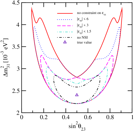
Figure 3.2: Allowed region in the $\sin^{2}\theta_{23}$-$\Delta m^{2}_{31}$-plane at 95% CL (2 d.o.f.). In this fit $\theta_{13}$, $\varepsilon_{e\tau}$ and $\varepsilon_{\tau\tau}$ are left free. The different lines correspond to different priors for the $\varepsilon_{\tau\tau}$ values as explained in the legend [10].

In summary, the inclusion of OPERA data helps only for very large values of $\varepsilon_{\tau\tau}$ as can be seen also from the first line of table 3.3. These large values, however are already excluded by the combination of MINOS and atmospheric results [117]. We checked that doubling the OPERA exposure does not change this conclusion. The slight improvement by OPERA is exclusively due to the $\nu_{\mu}$ sample in the muon tracker and the results do not change if we exclude the $\nu_{\tau}$ sample from the analysis. The usefulness of the $\nu_{\mu}$ sample stems from the very different value of $L/E$ compared to MINOS. These results are not too surprising, since even a very high energy neutrino factory will not be able to improve the bound on $\varepsilon_{\tau\tau}$ in comparison to atmospheric neutrino data [120].
B) Appearance: probing FC NSI ($\bm{\varepsilon_{e\tau}}$)
It is well known that, in the presence of NSI, the determination of $\theta_{13}$ exhibits a continuous degeneracy [109] between $\theta_{13}$ and $\varepsilon_{e\tau}$, which leads to a drastic loss in sensitivity in $\theta_{13}$. A measurement of only $P_{e\mu}$ and $P_{\bar{\mu}\bar{e}}$ at one $L/E$ cannot disentangle the two and will only yield a constraint on a combination of $\theta_{13}$ and $\varepsilon_{e\tau}$. In this context, it was shown in Ref. [111], that even a very rudimentary ability to measure $P_{\mu\tau}$ may be sufficient to break this degeneracy. Therefore, it seems natural to ask whether OPERA can improve upon the sensitivity for $\varepsilon_{e\tau}$ that can be reached only with MINOS. The latter has been studied in Ref. [117] in combination with atmospheric neutrinos and on its own in Ref. [118]. The result, basically, was that MINOS will not be able to break this degeneracy, and hence a possible $\theta_{13}$ bound from MINOS will, in reality, be a bound on a combination of $\varepsilon_{e\tau}$ and $\theta_{13}$.

In Tables 3.3 and 3.4 we display our results for a true value of $\theta_{13}=0$ and no NSI. The allowed range for $\varepsilon_{e\tau}$ shrinks only very little by the inclusion of OPERA data. As in the case of $\varepsilon_{\tau\tau}$ we checked that this result is not due to the $\nu_{\tau}$ sample in OPERA but is entirely due to the different $L/E$ compared to MINOS. Also a two-fold increase of the OPERA exposure does not substantially alter the result.

In order to improve the sensitivity to NSI and to break the degeneracy between $\theta_{13}$ and $\varepsilon_{e\tau}$ it will be necessary to get independent information on either $\varepsilon_{e\tau}$ or $\theta_{13}$. An improvement of direct bounds on $\varepsilon_{e\tau}$ is in principle possible by using a very high energy $\nu_{e}$ beam and a close detector, but this would require either a neutrino factory or a high $\gamma$ beta beam. Both these possibilities are far in the future and will therefore not be here considered any further. Thus, we focus on independent information on $\theta_{13}$. Reactor experiments are very sensitive to $\theta_{13}$ but do not feel any influence from $\varepsilon_{e\tau}$ since the baseline is very short and the energy very low which leads to negligible matter effects. This is true for standard MSW-like matter effects as well as non-standard matter effects due to NSI [142]. We consider here as new reactor experiment Double Chooz [132], but for our discussion Daya Bay [133] or RENO [143] would work equally well. In Fig. 3.3 we show the allowed regions in the $\sin 2\theta_{13}$-$\varepsilon_{e\tau}$ plane for the combinations of MINOS and Double Chooz (red solid curves) and of MINOS, Double Chooz and OPERA (blue dashed curves) for four different input values of $\sin^{2}2\theta_{13}$ indicated in the plot. As expected, the effect of Double Chooz in all four cases is to constrain the allowed $\sin 2\theta_{13}$ range. The impact of OPERA, given by the difference between the solid and dashed lines, is absent for very small true values of $\sin 2\theta_{13}$ and increases with increasing true values. For the largest currently permissible values of $\theta_{13}\simeq 0.16$, OPERA can considerably reduce the size of the allowed region and help to resolve the degeneracy. In that parameter region a moderate increase in the OPERA exposure would make it possible to constrain large negative values of $\varepsilon_{e\tau}$. Again, this effect has nothing to do with $\nu_{\tau}$ detection and, in this case, is based on the different $L/E$ in $\nu_{e}$-appearance channel.

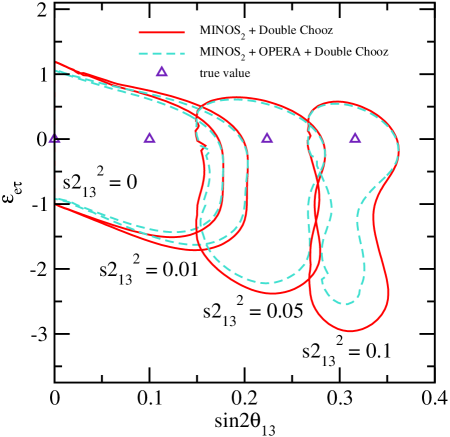
Figure 3.3: Allowed regions in the $\sin 2\theta_{13}$-$\varepsilon_{e\tau}$-plane at 95% CL (2 d.o.f.). $\Delta m^{2}_{31}$, $\theta_{23}$ and $\varepsilon_{\tau\tau}$ are left free in this fit. The solid lines correspond to the combination of MINOS₂ and Double Chooz while the dashed lines also include OPERA in the analysis. Each set of lines correspond to different true values for $\sin^{2}2\theta_{13}$, from left to right: 0, 0.01, 0.05 and 0.1 [10].

3.4.3 Conclusion

We have here studied how OPERA can help in improving the sensitivities on neutrino non-standard contact interactions of the third family of neutrinos. In our analysis we considered a combined OPERA fit together with high statistics MINOS data, in order to obtain restrictions on neutrino oscillation parameters in the presence of NSI. Due to its unique ability of detecting $\nu_{\tau}$ one would expect that the inclusion of OPERA data would provide new improved limits on the universality violating NSI parameter $\varepsilon_{\tau\tau}$. We found, however, that the $\nu_{\tau}$ data sample is too small to be of statistical significance. This holds even if we double the nominal exposure of OPERA to $9\times 10^{19}\,\mathrm{pot}$. OPERA also has a $\nu_{\mu}$ sample, which can help constraining NSI. Here the effect is due to the very different $L/E$ of OPERA compared to MINOS. This makes the OPERA $\nu_{\mu}$ sample more sensitive to NSI. However, the improvement is small and happens in a part of the NSI parameter space which is essentially excluded by atmospheric neutrino data.

We have also studied the possibility of constraining the FC NSI parameter $\varepsilon_{e\tau}$. For this purpose it is crucial to have a good knowledge of $\theta_{13}$. Therefore, we included future Double Chooz data, since reactor neutrino experiments are insensitive to the presence of NSI of the type considered here. Therefore, reactor experiments can provide a clean measurement of $\theta_{13}$, which in turn can be used in the analysis of long baseline data to probe the NSI. Double Chooz is only the first new reactor experiment and more precise ones like Daya Bay or Reno will follow. Our result would be qualitatively the same if we would have considered those, more precise, experiments, but clearly the numerical values of the obtained bounds would improve. The conclusion for $\varepsilon_{e\tau}$ with respect to the $\nu_{\tau}$ sample is the same as before: the sample is very much too small to be of any statistical significance. OPERA’s different $L/E$ again proves to be its most important feature and allows to shrink the allowed region on the $\sin^{2}\theta_{13}$-$\varepsilon_{e\tau}$ plane for large $\theta_{13}$ values. Here a modest increase in OPERA exposure would allow to completely lift the $\theta_{13}$-$\varepsilon_{e\tau}$ degeneracy and thus to obtain a unique solution.

	M2		O		M2+O
	90% C.L.	95% C.L.	90% C.L.	95% C.L.	90% C.L.	95% C.L.
$\varepsilon_{\tau\tau}$	[-10.8,10.8]	[-11.8,11.8]	[-10.4,10.4]	[-11.0,11.0]	[-8.5,8.5]	[-9.2,9.2]
$\varepsilon_{e\tau}$	[-1.9,0.9]	[-2.3,1.0]	[-2.1,1.4]	[-2.5,1.6]	[-1.6,0.9]	[-2.0,1.0]
$\Delta m^{2}_{31}$ [10-3 eV2]	[2.3,4.5]	[2.2,4.9]	[2.0,5.0]	[2.0,5.3]	[2.3,3.8]	[2.2,4.0]
$\sin^{2}\theta_{23}$	[0.08,0.92]	[0.07,0.93]	[0.08,0.92]	[0.07,0.93]	[0.12,0.88]	[0.11,0.89]

Table 3.3: 90% and 95% C.L. allowed regions for $\varepsilon_{\tau\tau}$, $\varepsilon_{e\tau}$, $\Delta m^{2}_{31}$ and $\sin^{2}\theta_{23}$ for different sets of experiments. Each row is obtained marginalizing over the remaining parameters in the table, plus $\theta_{13}$. The true value for $\sin^{2}2\theta_{13}$ is $0$ [10].

	M2		O		M2+O		M2+O+DC
	90% C.L.	95% C.L.	90% C.L.	95% C.L.	90% C.L.	95% C.L.	90% C.L.	95% C.L.
$\varepsilon_{\tau\tau}$	[-10.1,11.0]	[-11.2,12.0]	[-10.1,10.3]	[-10.8,11.0]	[-7.9,9.0]	[-8.7,9.6]	[-5.1,5.3]	[-5.6,5.8]
$\varepsilon_{e\tau}$	[-4.2,1.3]	[-4.5,1.5]	[-4.3,1.5]	[-5.0,1.8]	[-3.7,1.2]	[-4.1,1.4]	[-0.5,0.4]	[-0.7,0.5]
$\Delta m^{2}_{31}$ [10-3 eV2]	[2.3,4.6]	[2.2,5.0]	[2.0,4.8]	[2.0,5.2]	[2.3,4.0]	[2.2,4.2]	[2.3,2.8]	[2.3,2.9]
$\sin^{2}\theta_{23}$	[0.09,0.92]	[0.08,0.93]	[0.09,0.93]	[0.08,0.94]	[0.13,0.90]	[0.12,0.91]	[0.24,0.78]	[0.22,0.80]

Table 3.4: Same as table 3.3 with true value $\sin^{2}2\theta_{13}$ of $0.1$ [10].

Chapter 4 Collective Supernova Neutrino Transformations in Two Flavors

It is well known that neutrino interactions with the medium have a strong impact in their evolution, through the induced effective matter potentials $V_{\rm CC},~{}V_{\rm NC}$ and $V_{\mu\tau}$, as discussed in Chapter 2. What is not really well understood is the effect of neutrinos themselves, as a background medium. It was first pointed by Pantaleone [144] that the inclusion of neutrino-neutrino interaction into the problem would introduce an off-diagonal refractive index. The oscillation equations become then non-linear, leading sometimes to surprising collective phenomena in very dense environments such as the early Universe or core-collapse SNe.

Initially most of the attention was centered on the context of the early Universe, first in a series of papers by Samuel, Kostelecký and Pantaleone [145, 146, 147, 148, 149, 150, 151, 152, 153], and later by other authors [154, 155, 156, 157, 158]. But it was not until very recently that the community has realized the importance this ingredient might have in the frame of SN neutrinos [11, 12, 13, 159, 160, 161, 14, 162, 163, 164, 17, 15, 165, 166, 16, 167, 168, 19, 18, 169, 170, 171, 172, 173, 174, 175].

In the dense neutrino flux emerging from a SN core, neutrino-neutrino refraction causes non-linear flavor oscillation phenomena that are unlike anything produced by ordinary matter. There are several aspects that have to be taken into account when studying neutrino-neutrino interactions in the context of SN. The main two are multi-angle and multi-energy effects. On the one hand, neutrinos are not emitted from a single point but a spherical surface, the neutrino sphere. As a consequence, and due to the current-current nature of the weak interaction, neutrinos moving in different directions will experience a different refractive effect caused by the other neutrinos. On the other hand, the effect is energy dependent, and since SN neutrinos are emitted with a broad spectrum, this dependency could be an issue.

In this chapter we will address the question of multi-angle effects in SN neutrino transformations in a two flavor scenario, for both single and multi-energy configurations. But before we will review the main characteristics of the collective phenomena caused by the dense neutrino background.

4.1 Introduction

In order to study this complicated non-linear problem it is convenient to use the density matrix formalism. Mixed neutrinos are described by matrices of density $\varrho_{\bf p}$ and $\bar{\varrho}_{\bf p}$ for each (anti)neutrino mode, where overbarred quantities refer to antineutrinos here and now on. The diagonal entries are the usual occupation numbers whereas the off-diagonal terms encode phase information. The equations of motion (EOMs) are

$${\rm i}\partial_{t}\varrho_{\bf p}=[{\sf H}_{\bf p},\varrho_{\bf p}]\,,$$ (4.1)

where the Hamiltonian is [176]

$${\sf H}_{\bf p}=\Omega_{\bf p}+{\sf V}+\sqrt{2}\,G_{\rm F}\!\int\!\frac{{\rm d}^{3}{\bf q}}{(2\pi)^{3}}\left(\varrho_{\bf q}-\bar{\varrho}_{\bf q}\right)(1-{\bf v}_{\bf q}\cdot{\bf v}_{\bf p})\,,$$ (4.2)

${\bf v}_{\bf p}$ being the velocity of a neutrino mode with momentum ${\bf p}$. The matrix of vacuum oscillation frequencies is $\Omega_{\bf p}={\rm diag}(m_{1}^{2},m_{2}^{2},m_{3}^{2})/2|{\bf p}|$ in the mass basis. The matter effect is represented, in the weak interaction basis, by ${\sf V}=\sqrt{2}\,G_{\rm F}n_{B}\,{\rm diag}(Y_{e},0,Y_{\tau}^{\rm eff})$, as defined in Chapter 2. The factor $(1-{\bf v}_{\bf q}\cdot{\bf v}_{\bf p})=(1-\cos\theta_{\bf pq})$ represents the current-current nature of the weak interaction. For antineutrinos the only difference is $\Omega_{\bf p}\to-\Omega_{\bf p}$, i.e., in vacuum antineutrinos oscillate “the other way around”.

In the $\nu_{e}$-$\nu_{x}$ two-flavor system, the density matrices can be reduced to polarization vectors by using the Pauli matrices and the unit matrix. Therefore the EOMs can be reexpressed in terms of the polarization vectors using:

$$\varrho=\frac{1}{2}\left[P_{0}+{\bf P}\cdot{\bm{\sigma}}\right]~{},$$ (4.3)

where ${\bm{\sigma}}$ is the vector of Pauli matrices. In this formalism the survival probability of $\nu_{e}$ is given at time $t$ by $\frac{1}{2}[1+P_{z}(t)]$, and Eqs. (4.1) and (4.2) become

$$\dot{\bf P}_{\bf p}={\bf H}_{\bf p}\times{\bf P}_{\bf p}\,,$$ (4.4)

$${\bf H}_{\bf p}=\omega_{\bf p}{\bf B}+\lambda{\bf L}+\mu_{0}\int\frac{{\rm d}^{3}{\bf q}}{(2\pi)^{3}}\,\left({\bf P}_{\bf q}-\bar{\bf P}_{\bf q}\right)\left(1-{\bf v}_{\bf q}\cdot{\bf v}_{\bf p}\right)\,,$$ (4.5)

where $\omega_{\bf p}=|\Delta m^{2}/2E|$ is the vacuum oscillation frequency with $E=|{\bf p}|$ for relativistic neutrinos, ${\bf B}=(\sin 2\theta,0,\pm\cos 2\theta)$ is a unit vector in the mass direction in flavor space where the “$-$” sign corresponds to normal hierarchy and the “$+$” sign to inverted hierarchy, ${\bf L}$ is a unit vector in the weak-interaction direction with ${\bf B}\cdot{\bf L}=\cos 2\theta$ and $\theta$ the vacuum mixing angle. The effect of a homogeneous and isotropic medium is parameterized by

$$\lambda=\sqrt{2}\,G_{\rm F}(n_{e^{-}}-n_{e^{+}})\,,$$ (4.6)

where $n_{e^{\pm}}$ is the electron/positron number density. Finally the neutrino-neutrino term is given by

$$\mu_{0}=\sqrt{2}G_{\rm F}\left(F_{\bar{\nu}_{e}}^{R_{\nu}}-F_{\bar{\nu}_{x}}^{R_{\nu}}\right)\,,$$ (4.7)

where $F_{\bar{\nu}_{e}}^{R_{\nu}}$ and $F_{\bar{\nu}_{x}}^{R_{\nu}}$ are the $\bar{\nu}_{e}$ and $\bar{\nu}_{x}$ fluxes, taken at the neutrino sphere with radius $R_{\nu}$.

4.1.1 Single-angle and single-energy

Let us begin with the simplest case, single-angle and single-energy. We consider a two flavor system initially composed of equal densities of pure $\nu_{e}$ and $\bar{\nu}_{e}$, all of them emitted in the same direction with equal energies. The flavor content of these ensembles will be given by the polarization vectors in flavor space ${\bf P}$ and $\bar{\bf P}$. By definition, we take these vectors to be unitary.

In vacuum the general EOMs given by Eq. (4.4) are reduced for this system to

$$\partial_{t}{\bf P} = \left[+\omega{\bf B}+\mu\left({\bf P}-\bar{\bf P}\right)\right]\times{\bf P}\,,$$

$$\partial_{t}\bar{\bf P} = \left[-\omega{\bf B}+\mu\left({\bf P}-\bar{\bf P}\right)\right]\times\bar{\bf P}\,.$$ (4.8)

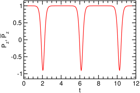
Figure 4.1: Evolution of $P_{z}$ and $\bar{P}_{z}$ for the system of equations Eq. (4.1.1) for inverted hierarchy, with $\theta=0.01$, $\omega=1$ km^-1, and a constant neutrino-neutrino interaction $\mu=10$ km^-1.

In Fig. 4.1 we show the evolution of $P_{z}$ and $\bar{P}_{z}$, given by Eq. (4.1.1), for a small vacuum mixing angle, inverted mass hierarchy and a constant $\mu$. Initially, both ${\bf P}$ and ${\bf\bar{P}}$ stay put. After some time, though, they flip completely, but immediately return to their original state, leading to periodic motion. This behavior, translated to flavor language, means that we obtain complete and simultaneous conversion of $\nu_{e}$ and $\bar{\nu}_{e}$ to $\nu_{\mu}$ and $\bar{\nu}_{\mu}$ and back. For the normal hierarchy on the other hand, nothing visible happens.

This evolution was proved in Ref. [14] to be equivalent to a pendulum in flavor space, by reducing the EOMs to those of a spherical pendulum. Making use of this analogy it is possible to explain why we only obtain bipolar conversion in the inverted hierarchy case. For normal hierarchy the system initially sets near the minimum of the pendulum potential and is therefore trapped leading to no visible effects. In the inverted hierarchy, conversely, the evolution starts with the system close to the maximum of the potential in an unstable equilibrium. Therefore it will always move to the minimum, leading to this periodic bipolar conversion. The bipolar period, i.e. the separation between dips, is obtained to scale logarithmically with the small vacuum mixing angle.

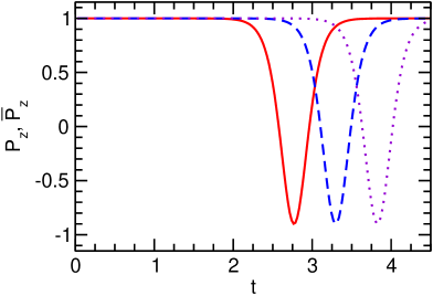
Figure 4.2: Evolution of $P_{z}$ and $\bar{P}_{z}$ in several systems with background matter described by Eq. (4.1.1). We are using inverted hierarchy, $\sin 2\theta=0.001$, $\omega=1$ km^-1, and $\mu=10$ km^-1 for all three systems. The red/solid line has $\lambda=10^{2}$, the blue/dashed line $\lambda=10^{3}$, and the violet/dotted line $\lambda=10^{4}$.

In the presence of a background medium of charged leptons the EOMs, Eq. (4.4), become:

$$\partial_{t}{\bf P} = \left[+\omega{\bf B}+\lambda{\bf L}+\mu\left({\bf P}-\bar{\bf P}\right)\right]\times{\bf P}\,,$$

$$\partial_{t}\bar{\bf P} = \left[-\omega{\bf B}+\lambda{\bf L}+\mu\left({\bf P}-\bar{\bf P}\right)\right]\times\bar{\bf P}\,.$$ (4.9)

As it was first pointed out by Duan et al. [159], by going to the frame co-rotating around the ${\bf L}$-direction we can reduce this equations to the ones in vacuum, Eq. (4.1.1), with a time dependent ${\bf B}$,

$${\bf B}=\left(\begin{array}[]{c}\sin(2\theta_{0})\cos(-\lambda t)\\ \sin(2\theta_{0})\sin(-\lambda t)\\ -\cos(2\theta_{0})\end{array}\right).$$ (4.10)

In this picture ${\bf B}$ rotates around the $z$-direction with frequency $-\lambda$. If this rotation is faster than all other frequencies one would naïvely expect that the transverse components of ${\bf B}$ average to zero, leaving us with $\langle{\bf B}\rangle$ along the $z$-axis, i.e., an effectively vanishing mixing angle and no flavor conversion. However, this fast rotating transverse components are still enough to trigger the conversion effect, with a matter suppressed effective mixing angle, though. Thus, the presence of matter in this simple picture is just to extend logarithmically the bipolar period. This is illustrated in Fig. 4.2. A more detailed description of the consequences of adding an ordinary matter background will be given in Sec. 4.4 for the multi-angle case.

In a realistic SN scenario the neutrino self-interaction strength is not constant. There is a radial dependence for the $\mu$ parameter. From the neutrino flux dilution we obtain a $r^{-2}$ scaling, but there will also be another $r^{-2}$ factor due to the collinearity suppression, coming from the $(1-{\bf v}_{\bf q}\cdot{\bf v}_{\bf p})$ factor in Eq. (4.2). These two effects leave us essentially with an $r^{-4}$ decline for the self-interaction term, see Appendix A for a more detailed description. We add now this neutrino density dependence, normalized at the neutrino sphere to $\mu_{0}\equiv\mu(R_{\nu})=7\times 10^{5}$ km^-1, to the previous picture: initial equal numbers of $\nu_{e}$ and $\bar{\nu}_{e}$ alone, inverted mass hierarchy and small mixing angle $\sin 2\theta=0.001$. We then find numerically the survival probability shown in Fig. 4.3. We obtain a decline of the oscillation amplitude as a function of radius leading to a complete flavor conversion caused by the bipolar effect. This result is to be compared with the periodic bipolar oscillations obtained in Fig. 4.1, with a constant $\mu$. This behavior can be understood using the pendulum analogy, Ref. [14]. The basic idea is that by reducing $\mu$ the energy of the system is also being reduced, so that, after the oscillation, the pendulum will not come back to its initial position (the maximum of the potential) but to a lower one, which will be closer and closer to the rest point as $\mu$ decreases.

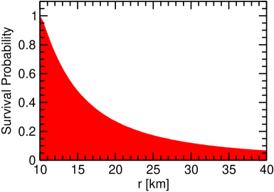
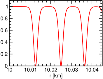
Figure 4.3: Survival probabilities for $\nu_{e}$ or $\bar{\nu}_{e}$ for a system with $\mu_{0}=7\times 10^{5}$ km^-1, $\sin 2\theta=0.001$ and symmetric initial conditions.

Another important feature to be taken into account in our way to simulate a realistic SN scenario, is the initial flux asymmetry obtained in typical SN numerical simulations. As described in Chapter 1, one expects the hierarchy of neutrino number fluxes $F^{R_{\nu}}_{\nu_{e}}>F^{R_{\nu}}_{\bar{\nu}_{e}}>F^{R_{\nu}}_{\nu_{x}}=F^{R_{\nu}}_{\bar{\nu}_{x}}$. We take this into account by imposing the initial conditions $\bar{P}_{z}=1$ and $P_{z}=1+\epsilon$, where the asymmetry parameter, $\epsilon$, represents the neutrino excess coming from the deleptonization of the collapsed core, and is defined as

$$\epsilon\equiv\frac{F^{R_{\nu}}_{\nu_{e}}-F^{R_{\nu}}_{\nu_{x}}}{F^{R_{\nu}}_{\bar{\nu}_{e}}-F^{R_{\nu}}_{\bar{\nu}_{x}}}-1=\frac{F^{R_{\nu}}_{\nu_{e}}-F^{R_{\nu}}_{\bar{\nu}_{e}}}{F^{R_{\nu}}_{\bar{\nu}_{e}}-F^{R_{\nu}}_{\bar{\nu}_{x}}}\,,$$ (4.11)

where we have used $F^{R_{\nu}}_{\nu_{x}}=F^{R_{\nu}}_{\bar{\nu}_{x}}$. We can assume $F^{R_{\nu}}_{\nu_{x}}=F^{R_{\nu}}_{\bar{\nu}_{x}}=0$ at the neutrino sphere without loss of generality, since flavor oscillations do not change those parts of the flavor fluxes that are already equal. Only the transformation of the excess $\bar{\nu}_{e}$ flux over the $\bar{\nu}_{x}$ flux is observable, and likewise for neutrinos.

Choosing $\epsilon=0.25$ and solving numerically the EOMs for this system, given in Eq. (4.1.1), we obtain the results shown in Fig. 4.4. We can distinguish different regimes of evolution, corresponding to different relative strengths of $\mu$ with respect to $\omega$. For large values of $\mu/\omega$, right behind the neutrino sphere and up to about 100 km, we observe a first stage of synchronized evolution where both neutrinos and antineutrinos stay in their original flavor. For intermediate values of $\mu/\omega$, after what we call $r_{\rm syn}$, we get a second stage of bipolar conversion, where complete pair transformations $\nu_{e}\bar{\nu}_{e}\to\nu_{x}\bar{\nu}_{x}$ are developed, keeping always the initial flavor lepton asymmetry conserved. The nutations we observe during this bipolar phase depend on the mixing angle, the smaller $\theta$ is, the larger the depth of the nutations. Beyond this point, small $\mu/\omega$, the neutrino-neutrino interactions die out and we obtain ordinary oscillations, where of course, normal matter will play an important role.

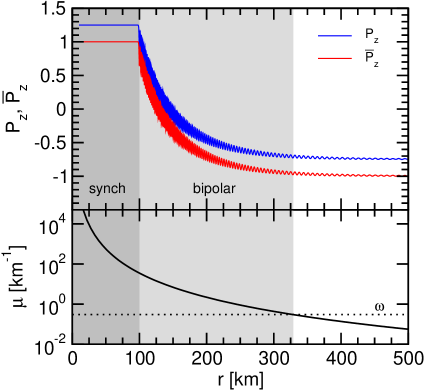
Figure 4.4: $P_{z}$ (blue) and $\bar{P}_{z}$ (red) evolution in our toy SN model with 25% more neutrinos than antineutrinos and $\sin 2\theta=0.001$. The grey shaded bands show the synchronization (dark) and bipolar regions (light).

The limiting condition between synchronized oscillations and bipolar conversions is found to be in Ref. [14]

$$\mu(r_{\rm syn})\simeq\frac{2\omega}{(1-\sqrt{1+\epsilon})^{2}}\,.$$ (4.12)

This means that for values of $\mu$ larger than this quantity synchronized evolution is obtained, while for smaller values is the turn of bipolar transformations. The end of this bipolar regime is determined by the condition,

$$\mu(r_{\rm bip})\simeq\omega,$$ (4.13)

thus for smaller values of $\mu$ no bipolar conversions are to be expected. In the single-angle case we find from Eq. (A.20) that the effective neutrino-neutrino interaction strength varies at large distances as

$$\mu_{\rm eff}(r)=\mu_{0}\,\frac{R_{\nu}^{4}}{2r^{4}}\,.$$ (4.14)

Therefore, the synchronization radius is

$$\frac{r_{\rm syn}}{R_{\nu}}=\left(\frac{\sqrt{1+\epsilon}-1}{2}\right)^{1/2}\left(\frac{\mu_{0}}{\omega}\right)^{1/4}\approx\frac{\sqrt{\epsilon}}{2}\,\left(\frac{\mu_{0}}{\omega}\right)^{1/4}\,.$$ (4.15)

The second line assumes $\epsilon\ll 1$. The bipolar radius on the other hand is given by

$$\frac{r_{\rm bip}}{R_{\nu}}=\left(\frac{\mu_{0}}{2\omega}\right)^{1/4}\,.$$ (4.16)

If we assume the values of the parameters used in Fig. 4.4: $\omega=0.3~{}{\rm km}^{-1}$, $\mu_{0}=7\times 10^{5}~{}{\rm km}^{-1}$, $R_{\nu}=10$ km and $\epsilon=0.25$, we find $r_{\rm syn}=95$ km and $r_{\rm bip}=330$ km corresponding well to the figure. For a typical Fe core SN the $H$- and $L$-resonances take place far outside this region, and therefore both effects are decoupled. Lower mass progenitors, though, may collapse with a O-Ne-Mg core. In this kind of SN the density profile may be such that both effects occur in the same region [168]. Throughout this thesis we will concentrate on the former case.

Changing the vacuum mixing angle and adding normal matter causes only the minor logarithmic changes discussed earlier. We illustrate this point in Fig. 4.5 with the evolution of $\bar{P}_{z}$ for the same case as in Fig. 4.4, but assuming now a large vacuum mixing angle $\sin 2\theta=0.1$. In the synchronization region one can now see oscillations. On the left panel of the top row, we overlay this curve with $\bar{P}_{z}$, using a typical matter profile, while on the right panel we superimpose the vacuum case with a reduced mixing angle. This reduced mixing angle is chosen to be the effective one at $r_{\rm syn}$ due to the matter profile used for the left panel. As expected, matter has the effect of slightly delaying the onset of pair transformations.

4.1.2 Single-angle and multi-energy

In addition to the radial dependence of $\mu$ and the initial neutrino-antineutrino asymmetry, another feature of SN neutrinos that plays an important role in this analysis is their energy spectra. As described in Chapter 1, far from being monochromatic, neutrinos are emitted from the star in a rather wide energy range, typically from 1 to 50 MeV. We need then to study the consequences of a multi-energy analysis.

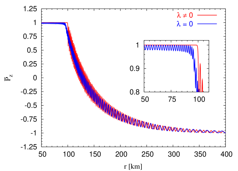
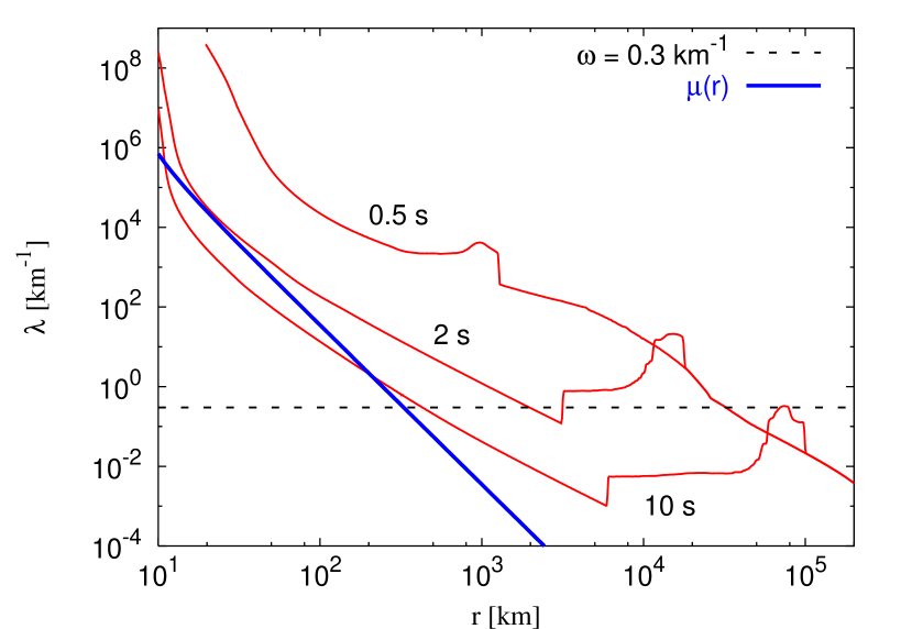
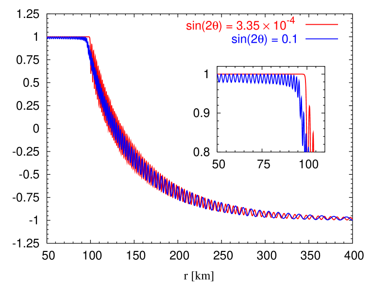
Figure 4.5: Top: Same case as in Fig. 4.4 but for large vacuum mixing angle of $\sin 2\theta=0.1$ (blue in both panels), compared with different ways of suppressing the mixing angle (red). Left: ordinary matter according to the profile at $t=2\,$s in bottom panel, where typical profiles of Garching group [177] plus $\mu(r)$ are shown. Right: small vacuum mixing angle of $\sin 2\theta=3.35\times 10^{-4}$ [17].

Let us start considering the evolution of an ensemble consisting of only neutrinos with many momenta, $p_{j}$. In this case the general EOMs, Eq. (4.4), can be written for each mode as

$$\partial_{t}{\bf P}_{j}=\left(\omega_{j}{\bf B}+\mu{\bf J}\right)\times{\bf P}_{j}\,,$$ (4.17)

analogously to Eq. (4.1.1), where $\omega_{j}\equiv\Delta m^{2}/2p_{j}$. We have defined the polarization vector for the entire ensemble as

$${\bf J}\equiv\sum_{j=1}^{N_{\nu}}{\bf P}_{j}\,,$$ (4.18)

$N_{\nu}$ being the number of neutrino modes. In the well known case where we do not consider neutrino-neutrino interactions, or these are too weak, each energy mode oscillates around ${\bf B}$ with its particular frequency $\omega_{j}$. This behavior leads inevitably to a quick decoherence. The effect is illustrated in Fig. 4.6 for an ensemble of neutrinos with a thermal momentum distribution at temperature $T$. The vacuum mixing angle was taken to be $\sin 2\theta=0.8$ and all neutrinos were originally in a pure $\nu_{e}$ state.

Figure 4.6: Total $\nu_{e}$ survival probability as a function of time, where $\tau\equiv(\Delta m^{2}/2p_{0})t$ and $p_{0}=\langle p^{-1}\rangle^{-1}\simeq 2.2\,T$. The curves are for different values $\kappa\equiv\mu/(\Delta m^{2}/2p_{0})$ of the neutrino self-coupling as indicated where $\kappa=0$ corresponds to vacuum oscillations [154].

The situation changes, though, if we consider a sufficiently dense neutrino ensemble [154]. In such a case all neutrino modes oscillate together with a common $synchronized$ frequency. This leads to a net oscillation effect for the whole neutrino ensemble, as shown in Fig. 4.6. In this case, we can no longer neglect the second term in Eq. (4.17).

This effect can be intuitively understood by looking at the EOMs, Eq. (4.17). We see two different oscillatory components. On the one hand each individual mode precesses around ${\bf B}$ with a particular $\omega_{j}$, on the other hand all of them precess around the global polarization vector ${\bf J}$ with a common frequency. Of course, ${\bf J}$ is not a constant vector, but depends on the behavior of ${\bf P}_{j}$. If we sum Eq. (4.17) over all modes we obtain

$$\dot{\bf J}={\bf B}\times\sum_{j=1}^{N_{\nu}}\omega_{j}{\bf P}_{j}.$$ (4.19)

Therefore, if the precession frequency around ${\bf J}$ is much larger than the one around ${\bf B}$, i.e. if $\mu$ is sufficiently large and changes sufficiently slowly (adiabatic limit [165]), the evolution of a given mode remains dominated by ${\bf J}$. The fast precession around ${\bf J}$ implies that the projection of ${\bf P}_{j}$ on ${\bf J}$ is conserved while the transverse component averages to zero on a fast time scale relative to the slow precession around ${\bf B}$. If ${\bf J}$ moves slowly, then the individual modes will follow ${\bf J}$. Of course, if the external field is much larger than the internal ones (dilute neutrino gas), then the modes will decouple and precess individually around the external field with their separate vacuum oscillation frequencies.

We can now derive the synchronization frequency that leads the evolution of the compound system,

$$\dot{\bf J}=\omega_{\rm syn}\,{\bf B}\times{\bf J}.$$ (4.20)

Of the individual modes, the external field “sees” only the projection along ${\bf J}$ because the transverse components average to zero. One can define here an effective magnetic moment, ${\bf M}$, of the system, obtaining that the contribution of mode $j$ to this total magnetic moment is $\omega_{j}\,{\bf\hat{J}}\cdot{\bf P}_{j}$ so that

$${\bf M}={\bf\hat{J}}\,\sum_{j=1}^{N_{\nu}}\omega_{j}\,{\bf\hat{J}}\cdot{\bf P}_{j},$$ (4.21)

where ${\bf\hat{J}}$ is a unit vector in the direction of ${\bf J}$. And we therefore obtain

$$\omega_{\rm syn}=\frac{|{\bf M}|}{|{\bf J}|}=\frac{1}{|{\bf J}|}\sum_{j=1}^{N_{\nu}}\omega_{j}\,{\bf\hat{J}}\cdot{\bf P}_{j}.$$ (4.22)

In particular, if all modes started aligned (coherent flavor state) then $|{\bf J}|=N_{\nu}$ and ${\bf\hat{J}}\cdot{\bf P}_{j}=1$ so that

$$\omega_{\rm syn}=\left\langle\omega\right\rangle=\frac{1}{N_{\nu}}\sum_{j=1}^{N_{\nu}}\frac{\Delta m^{2}}{2p_{j}}=\frac{\Delta m^{2}}{2}\langle\frac{1}{p}\rangle.$$ (4.23)

Let us study now the case where neutrinos and antineutrinos are simultaneously present, with a continuum of energy modes. Therefore, all the summations in the quantities defined previously will become integrals. We can then define ${\bf J}=\int_{0}^{\infty}d\omega\,{\bf P}_{\omega}$ and $\bar{\bf J}=\int_{0}^{\infty}d\omega\,\bar{\bf P}_{\omega}$ and introduce ${\bf D}\equiv{\bf J}-\bar{\bf J}$, representing the net lepton number. The equivalent EOMs to those of Eq. (4.1.1) are now

$$\partial_{t}{\bf P}_{\omega} = \left(+\omega{\bf B}+\mu{\bf D}\right)\times{\bf P}_{\omega}\,,$$

$$\partial_{t}\bar{\bf P}_{\omega} = \left(-\omega{\bf B}+\mu{\bf D}\right)\times\bar{\bf P}_{\omega}\,.$$ (4.24)

As discussed earlier, the only difference between the equations for neutrinos and antineutrinos is the sign in the vacuum term. This suggests the use of a more compact notation, where we use only ${\bf P}_{\omega}$ by extending it to negative frequencies such that $\bar{\bf P}_{\omega}={\bf P}_{-\omega}$ ($\omega>0$). The EOMs take then the very same form as Eq. (4.17)

$$\dot{\bf P}_{\omega}=\left(\omega{\bf B}+\mu{\bf D}\right)\times{\bf P}_{\omega}\,.$$ (4.25)

The difference vector is then redefined as

$${\bf D}=\int_{-\infty}^{+\infty}d\omega\,s_{\omega}\,{\bf P}_{\omega},$$ (4.26)

where $s_{\omega}\equiv{\rm sign}(\omega)=\omega/|\omega|$. Integrating both sides of Eq. (4.25) over $s_{\omega}d\omega$ provides

$$\dot{\bf D}={\bf B}\times{\bf M}\,,$$ (4.27)

where

$${\bf M}\equiv\int_{-\infty}^{+\infty}d\omega\,s_{\omega}\omega\,{\bf P}_{\omega}$$ (4.28)

is again the effective magnetic moment of the system.

We have obtained a completely analogous situation to the neutrino-only case. Here both neutrinos and antineutrinos behave in the same way if $\mu$ is sufficiently large, and therefore ${\bf M}\propto{\bf D}$. As a consequence, and making use of Eq. (4.27), we see how ${\bf D}$ precesses around ${\bf B}$ with the synchronization frequency

$$\omega_{\rm syn}=\frac{|{\bf M}|}{|{\bf J}|}=\frac{\int_{-\infty}^{+\infty}d\omega\,s_{\omega}\omega\,P_{\omega}}{\int_{-\infty}^{+\infty}d\omega\,P_{\omega}}\,,$$ (4.29)

which is just the generalization of Eq. (4.22).

So, just as in the neutrino-only case, we obtain that a multi-energy ensemble behaves as if all neutrinos had a common vacuum oscillation frequency given by Eq. (4.29). Therefore the evolution of a neutrino and antineutrino ensemble with an energy spectrum will be basically the same discussed in Sec. 4.1.1, with a vacuum oscillation frequency $\omega_{\rm syn}$.

After this generic discussion on the multi-energy case, let us concentrate again on the specific scenario of interest, a SN with varying $\mu$ and flavor asymmetry $\epsilon$. Although the evolution of the system is basically the same discussed for the single-energy situation, as we have just deduced, there is one special feature characteristic of such a system, namely the spectral split. This effect was first numerically observed by Duan et al. [160, 161] and later on discussed in the context of two flavors by Raffelt and Smirnov [15, 165], Fogli et al. [16], and in three flavors by Duan et al. [170] and Dasgupta et al. [19]. The main result is shown in Fig. 4.7, taken from Ref. [165]. Represented with thin lines are the thermal $\nu_{e}$ and $\bar{\nu}_{e}$ flux spectra with an average energy of 15 MeV produced in the neutrino sphere of a SN core. The mean energies are chosen to be equal while the $\nu_{e}$ flux is 25$\%$ larger than the $\bar{\nu}_{e}$ flux and the other fluxes are completely ignored. With thick lines are shown the emerging spectra, once neutrino-neutrino interactions can be neglected. On the one hand we observe how the antineutrino spectra (dashed line) has completely flipped, converting to the x-flavor. On the other hand a twofold behavior is observed for neutrinos (solid), all of them above a characteristic energy ($E_{\rm split}$) convert also to the x-flavor, while the ones below $E_{\rm split}$ stay in their original state.

Figure 4.7: Neutrino spectra at the neutrino sphere (thin lines) and beyond the dense-neutrino region (thick lines) for the schematic SN model described in the text. Solid: neutrinos. Dashed: antineutrinos. Positive spectrum: electron (anti)neutrinos. Negative spectrum: $x$ (anti)neutrinos.

To understand this result we will follow the description given in Ref. [165]. We rewrite the EOMs for this system in terms of an effective Hamiltonian

$$\partial_{t}{\bf P}_{\omega}={\bf H}_{\omega}\times{\bf P}_{\omega}\,,$$ (4.30)

where

$${\bf H}_{\omega}=\omega{\bf B}+\mu{\bf D}.$$ (4.31)

As described previously, in the adiabatic limit ${\bf P}_{\omega}$ will precess around ${\bf H}_{\omega}$ following at the same time its movement. We assume the usual situation in which all neutrinos are initially in the same state, all of ${\bf P}_{\omega}$ pointing in the direction of ${\bf H}_{\omega}$ due to the large initial $\mu$. Therefore, in the adiabatic limit they stay aligned with ${\bf H}_{\omega}$ for the entire evolution:

$${\bf P}_{\omega}(\mu)=\hat{\bf H}_{\omega}(\mu)\,P_{\omega}\,,$$ (4.32)

which solves the EOMs. Here $P_{\omega}\equiv|{\bf P}_{\omega}|$ and $\hat{\bf H}_{\omega}\equiv{\bf H}_{\omega}/|{\bf H}_{\omega}|$ is a unit vector. As usual we assume an excess flux of neutrinos over antineutrinos, implying that initially ${\bf P}_{\omega}$ and ${\bf D}$ are collinear and $D_{z}>0$.

In the adiabatic limit then, all ${\bf P}_{\omega}$ will have the same direction as ${\bf H}_{\omega}$, which in turn will be confined to the ${\bf B}-{\bf D}$ plane, as given in Eq. (4.31). As a consequence ${\bf M}$ will also stay in that plane, allowing us to redefine it as

$${\bf M}=b\,{\bf B}+\omega_{\rm c}{\bf D}$$ (4.33)

and rewrite the EOM of Eq. (4.27) as

$$\partial_{t}{\bf D}=\omega_{\rm c}\,{\bf B}\times{\bf D}.$$ (4.34)

The system is therefore evolving simultaneously in two ways: a fast precession around ${\bf B}$ determined by $\omega_{\rm c}=\omega_{\rm c}(\mu)$ and a drift in the co-rotating plane caused by the explicit $\mu(t)$ variation. If we go to the co-rotating frame, the individual Hamiltonians become

$${\bf H}_{\omega}=(\omega-\omega_{\rm c})\,{\bf B}+\mu{\bf D}\,.$$ (4.35)

We can now see how the system evolves with the decrease of $\mu$. Initially ($\mu\to\infty$) the oscillations are synchronized, $\omega_{\rm c}^{\infty}=\omega_{\rm syn}$, and all ${\bf P}_{\omega}$ form a collective ${\bf P}$. As $\mu$ decreases, the ${\bf P}_{\omega}$ zenith angles spread out while remaining in a single co-rotating plane. In the end ($\mu\to 0$) the co-rotation frequency is $\omega_{\rm c}^{0}$ and Eqs. (4.32) and (4.35) imply that all final ${\bf H}_{\omega}$ and therefore all ${\bf P}_{\omega}$ with $\omega>\omega_{\rm c}^{0}$ are aligned with ${\bf B}$, the others anti-aligned: a spectral split is inevitable with $\omega_{\rm split}\equiv\omega_{\rm c}^{0}$ being the split frequency. The lengths $P_{\omega}=|{\bf P}_{\omega}|$ are conserved and eventually all ${\bf P}_{\omega}$ point in the $\pm{\bf B}$ directions. Therefore the conservation of flavor-lepton number gives us $\omega_{\rm split}$, for $D_{z}>0$, by virtue of

$$D_{z}=\int_{-\infty}^{0}P_{\omega}\,d\omega-\int_{0}^{\omega_{\rm split}}P_{\omega}\,d\omega+\int_{\omega_{\rm split}}^{+\infty}P_{\omega}\,d\omega\,.$$ (4.36)

In general, $\omega_{\rm split}=\omega_{\rm c}^{0}\neq\omega_{\rm c}^{\infty}=\omega_{\rm syn}$.

It appears naturally from this explanation that the spectral split will take place only for neutrinos or antineutrinos, depending on which of them has the largest flux. As a particular case, there would be no spectral split for equal neutrino and antineutrino fluxes.

4.2 Multi-angle analysis. Equations of motion

As described in the introduction, the question we want to address in this chapter is the consequences of the multi-angle analysis in the evolution of SN neutrinos, for both single and multi-energy cases. This kind of neutrinos are not emitted from a single point, but from the neutrino sphere, which can be approximated as a spherical surface. The EOMs will therefore be affected by the geometry of the problem, including an angular dependence.

Our fundamental quantities are the flux matrices in flavor space ${\sf J}_{r}$ that depend on the radial coordinate $r$ (Appendix A). The diagonal entries represent the total neutrino number fluxes through a sphere of radius $r$. In the absence of oscillations, ${\sf J}_{r}$ would not depend on the radius at all. The flux matrices are represented by polarization vectors ${\bf P}_{r}$ in the usual way,

$${\sf J}_{r} = \frac{F^{R_{\nu}}_{\nu_{e}}+F^{R_{\nu}}_{\nu_{x}}}{2}+\frac{F^{R_{\nu}}_{\bar{\nu}_{e}}-F^{R_{\nu}}_{\bar{\nu}_{x}}}{2}\,{\bf P}_{r}\cdot\bm{\sigma}\,,$$

$$\bar{\sf J}_{r} = \frac{F^{R_{\nu}}_{\bar{\nu}_{e}}+F^{R_{\nu}}_{\bar{\nu}_{x}}}{2}+\frac{F^{R_{\nu}}_{\bar{\nu}_{e}}-F^{R_{\nu}}_{\bar{\nu}_{x}}}{2}\,\bar{\bf P}_{r}\cdot\bm{\sigma}\,,$$ (4.37)

where $\bm{\sigma}$ is the vector of Pauli matrices. The number fluxes $F^{R_{\nu}}_{\nu}$ are understood at the neutrino sphere, as always. In both equations the term proportional to the polarization vector is normalized to the antineutrino flux. As a consequence, at the neutrino sphere we have the normalization

$$P=|{\bf P}|=1+\epsilon\hbox{\quad and\quad}\bar{P}=|\bar{\bf P}|=1\,.$$ (4.38)

where $\epsilon$ is the asymmetry parameter defined in Eq. (4.11). In this way, we treat the excess flux from deleptonization as an adjustable parameter without affecting the baseline flux of antineutrinos,.

The diagonal part of the flux matrices is conserved and irrelevant for flavor oscillations. The polarization vector ${\bf P}_{r}$ only captures the difference between the flavor fluxes. For this reason we have defined the asymmetry $\epsilon$ in terms of the flux differences.

We want to study here multi-angle effects. For the geometry we are considering, it is convenient to label the different angular modes with

$$u=\sin^{2}\vartheta_{R}\,,$$ (4.39)

where $\vartheta_{R}$ is the zenith angle at the neutrino sphere $r=R_{\nu}$ of a given mode relative to the radial direction, see Fig. 4.8. The parameter $u$ is fixed for every trajectory whereas the physical zenith angle $\vartheta_{r}$ at distance $r$ varies. Therefore, using the local zenith angle to label the modes would complicate the equations.

Figure 4.8: Schematic neutrino emission in a spherical symmetric system. The solid line represents a neutrino emitted from the neutrino sphere ($R_{\nu}$) at an angle $\theta_{R}$ relative to the normal direction. This neutrino intersects the radial axis at point $P$ at distance $r$ from the center of the star, forming an angle $\theta_{r}$ with the axis. The system therefore satisfies $R_{\nu}\sin\theta_{R}=r\sin\theta_{r}$. Point $P$ sees only neutrinos traveling within the cone delimited by the dotted lines. Figure adapted from [160].

We will consider two generic angular distributions for the modes. In the multi-angle case we assume that the neutrino radiation field is “half isotropic” directly above the neutrino sphere, i.e., all outward moving modes are equally occupied as expected for blackbody emission. This implies (Appendix A)

$${\bf P}_{u,r}={\rm d}{\bf P}_{r}/{\rm d}u={\rm const.}$$ (4.40)

at $r=R_{\nu}$ for $0\leq u\leq 1$. Note that $u=0$ represents radial modes, $u=1$ tangential ones. The other generic distribution is the single-angle case where all neutrinos are taken to be launched at $45^{\circ}$ at the neutrino sphere so that $u=1/2$ for all neutrinos. This is a very interesting case, because as we will later see it seems to catch the whole physics of the problem. Moreover, from a more practical point of view, this approximation saves a lot of numerical effort.

For a monochromatic energy distribution, the EOMs in spherical symmetry are (Appendix A)

$$\partial_{r}{\bf P}_{u,r} = +\frac{\omega{\bf B}\times{\bf P}_{u,r}}{v_{u,r}}+\frac{\lambda_{r}{\bf L}\times{\bf P}_{u,r}}{v_{u,r}}+$$

$$\mu_{0}\,\frac{R_{\nu}^{2}}{r^{2}}\left[\left(\int_{0}^{1}{\rm d}u^{\prime}\,\frac{{\bf P}_{u^{\prime},r}-\bar{\bf P}_{u^{\prime},r}}{v_{u^{\prime},r}}\right)\times\left(\frac{{\bf P}_{u,r}}{v_{u,r}}\right)-({\bf P}_{r}-\bar{\bf P}_{r})\times{\bf P}_{u,r}\right]\,,$$

$$\partial_{r}\bar{\bf P}_{u,r} = -\frac{\omega{\bf B}\times\bar{\bf P}_{u,r}}{v_{u,r}}+\frac{\lambda_{r}{\bf L}\times\bar{\bf P}_{u,r}}{v_{u,r}}+$$

$$\mu_{0}\,\frac{R_{\nu}^{2}}{r^{2}}\left[\left(\int_{0}^{1}{\rm d}u^{\prime}\,\frac{{\bf P}_{u^{\prime},r}-\bar{\bf P}_{u^{\prime},r}}{v_{u^{\prime},r}}\right)\times\left(\frac{\bar{\bf P}_{u,r}}{v_{u,r}}\right)-({\bf P}_{r}-\bar{\bf P}_{r})\times\bar{\bf P}_{u,r}\right]\,,$$

where the radial velocity of mode $u$ at radius $r$ is

$$v_{u,r}=\sqrt{1-u\,R_{\nu}^{2}/r^{2}}\,.$$ (4.42)

The radial velocity in Eq. (4.2) introduces a relative strength factor for the different angular modes. As a consequence, one would expect two sources of kinematical decoherence, the self-interaction term and the matter term. We do not consider the vacuum term as a possible source for decoherence because by the time this term is dominant neutrinos are basically collinear. It seems important then to study the self-induced neutrino decoherence and the role of dense matter in collective SN neutrino transformations.

4.3 Decoherence in supernova neutrino transformations suppressed by deleptonization

The current-current nature of the weak interaction causes the interaction energy to depend on $(1-\cos\theta)$ for two trajectories with relative angle $\theta$. Therefore, neutrinos emitted in different directions from a SN core experience different refractive effects [160, 161]. As a result, one would expect that their flavor content evolves differently, leading to kinematical decoherence between different angular modes [12]. In the SN context, however, it has been numerically observed that the evolution is similar to the single-angle (or the isotropic) case [160, 161]. We analyze here up to which extent this approximation is valid and study the role of the different model parameters on the decoherence coming from multi-angle effects.

In Ref. [164] it was shown that this multi-angle decoherence is indeed unavoidable in a “symmetric gas” of equal densities of neutrinos and antineutrinos. Moreover, this effect is self-accelerating in that an infinitesimal anisotropy is enough to trigger an exponential run-away towards flavor equipartition, both for the normal and inverted hierarchies. Therefore, the observed suppression of multi-angle decoherence must be related to the $\nu_{e}\bar{\nu}_{e}$ asymmetry that is generated by SN core deleptonization.

To illustrate this point we show in Fig. 4.9 a few examples along the lines of Fig. 4.4, but now for multi-angle emission from the neutrino sphere that is again taken at 10 km. We consider different values of the asymmetry parameter. The left panels are for the normal hierarchy, the right panels for the inverted hierarchy. Since $P_{z}(r)-\bar{P}_{z}(r)=\epsilon$ is constant, it is sufficient to show $\bar{P}_{z}(r)$ alone. However, the length $\bar{P}=|\bar{\bf P}|$ is no longer preserved: Complete kinematical decoherence among the angular modes would cause $\bar{P}=0$. On the other hand, if $\bar{P}=1$ remains fixed, this signifies that all modes evolve coherently with each other. We use $\bar{\bf P}$ rather than ${\bf P}$ because the former measures what happens to the $\nu_{e}\bar{\nu}_{e}$ pairs, whereas the latter also includes the conserved $\nu_{e}$ excess.

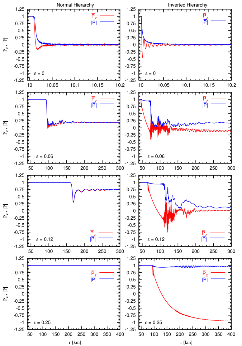
Figure 4.9: Radial evolution of $\bar{P}_{z}$ in a schematic SN model as in Fig. 4.4, but now for multi-angle neutrino emission at the neutrino sphere ($R_{\nu}=10$ km). In addition we show the length $\bar{P}=|\bar{\bf P}|$ as a measure of kinematical coherence. Left: normal hierarchy. Right: inverted hierarchy. From top to bottom: $\epsilon=0$, 0.06, 0.12 and 0.25, where $\epsilon$ is defined in Eq. (4.11) [17].

In the top row we use $\epsilon=0$ (symmetric case). The flavor content decoheres quickly in agreement with Ref. [164]. Both the length and the $z$-components of ${\bf P}$ and $\bar{\bf P}$ shrink to zero within about 20 meters of the nominal neutrino sphere.

On the other extreme, we show in the bottom row the same for $\epsilon=0.25$. In the normal hierarchy, nothing visible happens, in analogy to the single-angle case. In the inverted hierarchy, the transformation is similar, but not identical, to the single-angle case. The nutations wash out quickly. Shortly after exiting from the synchronization phase, the length $\bar{P}$ shrinks a bit, but stays almost constant thereafter. Clearly, some sort of multi-angle effect has happened as we will discuss further in Sec. 4.3.2, but multi-angle decoherence has certainly not occurred.

In the two middle rows we show intermediate cases with $\epsilon=0.06$ and 0.12, respectively. For the inverted hierarchy, these examples are qualitatively equivalent. The evolution is at first similar to the single-angle case and analogous to $\epsilon=0.25$. The nutations are washed out and the length $\bar{P}$ shrinks a little bit after the synchronization radius. At some larger radius, however, something new happens in that $\bar{P}$ suddenly shrinks significantly, although not to zero, and there is a distinct feature in the evolution of the $z$-component. Now we obtain partial decoherence. The final flavor content is very different from the single-angle case.

In the normal hierarchy, and for $\epsilon=0.06$, we obtain large decoherence that begins abruptly at some radius far beyond $r_{\rm syn}$. For the larger asymmetry $\epsilon=0.12$, the length $\bar{P}$ also shrinks, but closely tracks $\bar{P}_{z}$. As we will see, this case is somewhat like the second stage of the inverted-hierarchy case, i.e., a certain amount of shrinking of the length of $\bar{P}$ and thus a clear multi-angle effect, but no real decoherence.

Depending on the deleptonization flux, here represented by the asymmetry parameter $\epsilon$, the system behaves very differently. In particular, for the inverted hierarchy it is striking that there are either two or three distinct phases. We always have the initial synchronized phase at large neutrino densities. Next, there is always the quasi single-angle pair-transformation phase at distances larger than $r_{\rm syn}$. Just beyond this radius, the global polarization vectors quickly shrink by a small amount, but then stabilize immediately. Finally, if $\epsilon$ is below some critical value, there is a sharp transition to a third phase where the different angular modes decohere significantly, but not completely. The practical outcome for the flavor fluxes emerging from the dense-neutrino region is very different depending on $\epsilon$. The transition between these regimes is abrupt, a small change of $\epsilon$ is enough to cause one or the other form of behavior.

4.3.1 Setup of the problem

In the previous section we have presented the different regimes of evolution due to multi-angle effects. Let us now try to understand this behavior.
A) Schematic supernova model
We will here consider a two-flavor oscillation scenario driven by the atmospheric $\Delta m^{2}=1.9$–$3.0\times 10^{-3}~{}{\rm eV}^{2}$. Assuming $\langle E_{\nu}\rangle=15$ MeV, the oscillation frequency is $\omega=\hbox{0.3--0.5}~{}{\rm km}^{-1}$. To be specific, we use

$$\omega=\left\langle\frac{\Delta m^{2}}{2E}\right\rangle=0.3~{}{\rm km}^{-1}$$ (4.43)

as a benchmark value in the monochromatic model.

The total energy output of a SN is around $3\times 10^{53}~{}{\rm erg}$, corresponding to $0.5\times 10^{53}~{}{\rm erg}$ in each of the six neutrino species if we assume approximate equipartition of the emitted energy. If this energy is emitted over 10 s, the average luminosity per flavor would be $0.5\times 10^{52}~{}{\rm erg/s}$. However, at early times during the accretion phase, the luminosity in the $\bar{\nu}_{e}$ flavor can exceed $3\times 10^{53}~{}{\rm erg/s}$ [178]. As our baseline estimate we use

$$\mu_{0}=7\times 10^{5}~{}{\rm km}^{-1}\times\left(\frac{L_{\bar{\nu}_{e}}}{\langle E_{\bar{\nu}_{e}}\rangle}-\frac{L_{\bar{\nu}_{x}}}{\langle E_{\bar{\nu}_{x}}\rangle}\right)\frac{15~{}{\rm MeV}}{10^{52}~{}{\rm erg/s}}\,\left(\frac{10~{}{\rm km}}{R_{\nu}}\right)^{2}\,.$$ (4.44)

Unless otherwise stated, throughout this section we always use the benchmark values for the different parameters summarized in Table 4.1.

Table 4.1: Default values for our model parameters.

Parameter	Standard value	Definition
$\epsilon$	0.25	Eq. (4.11)
$\mu_{0}$	$7\times 10^{5}~{}{\rm km}^{-1}$	Eq. (4.7)
$\omega$	$0.3~{}{\rm km}^{-1}$	Eq. (4.43)
$\sin 2\theta$	$10^{-3}$	—

In our calculations we always take the neutrino sphere at the radius $R_{\nu}=10$ km. Of course, the physical neutrino sphere is not a well-defined concept. Therefore, the radius $R_{\nu}$ simply represents the location where we fix the inner boundary condition. However, essentially nothing happens until the synchronization radius $r_{\rm syn}\gg R_{\nu}$ because the in-medium mixing angle is extremely small and both neutrinos and antineutrinos simply precess around ${\bf B}$. Therefore, as far as the vacuum and matter oscillation terms are concerned, it is almost irrelevant where we fix the inner boundary condition.

Not so for the neutrino-neutrino term because we also fix the angular distribution at $r=R_{\nu}$. While the $r^{-2}$ scaling from flux dilution is unaffected by the radius for the inner boundary condition, the “collinearity suppression” also scales as $(R_{\nu}/r)^{2}$ for $r\gg R_{\nu}$. If we fix a half-isotropic distribution or a single angle of $45^{\circ}$ at a larger radius $R_{\nu}^{\prime}$, the new inner boundary condition essentially amounts to $\mu_{0}\to\mu^{\prime}_{0}=\mu_{0}\,(R_{\nu}^{\prime}/R_{\nu})^{2}$. In the early phase after bounce $R_{\nu}^{\prime}=30$ km could be more realistic, leading to a $\mu_{0}$ value almost an order of magnitude larger. Evidently, $\mu_{0}$ is a rather uncertain model parameter that can differ by orders of magnitude from our benchmark value.

However, collective pair conversions only begin at $r_{\rm syn}$ where $\mu$ is so small that synchronization ends. Therefore, the main impact of a modified $\mu_{0}$ is to change $r_{\rm syn}$ and thus to push the collective pair conversions to larger radii. In any event, according to Eq. (4.15) if $\mu_{0}$ is taken to be uncertain by two orders of magnitude, $r_{\rm syn}$ only changes by a factor of 3.

The total electron lepton number emitted from a collapsed SN core is about $3\times 10^{56}$. On the other hand, assuming that each neutrino species carries away $0.5\times 10^{53}~{}{\rm erg}$ with an average energy of 15 MeV, the SN core emits about $2\times 10^{57}$ neutrinos in each of the six species. In this simplified picture, the SN emits on average about 15% more $\nu_{e}$ than $\bar{\nu}_{e}$. However, in the oscillation context we need the excess of $F^{R_{\nu}}_{\nu_{e}}-F^{R_{\nu}}_{\nu_{x}}$ relative to the same quantity for antineutrinos as defined in Eq. (4.11). The true value of $\epsilon$ thus depends sensitively on the detailed fluxes and spectra of the emitted neutrinos. The asymmetry parameter is large when the first hierarchy in $F^{R_{\nu}}_{\nu_{e}}>F^{R_{\nu}}_{\bar{\nu}_{e}}>F^{R_{\nu}}_{\bar{\nu}_{x}}=F^{R_{\nu}}_{\nu_{x}}$ is large and/or the second hierarchy is small. Even if $F^{R_{\nu}}_{\bar{\nu}_{x}}$ is as small as half of $F^{R_{\nu}}_{\bar{\nu}_{e}}$, the asymmetry $\epsilon$ would be as large as 30%, even when $F^{R_{\nu}}_{\nu_{e}}$ exceeds $F^{R_{\nu}}_{\bar{\nu}_{e}}$ by only 15%.
B) Numerical multi-angle decoherence and the inner boundary condition
One important and somewhat confusing complication of numerically solving the EOMs is the phenomenon of numerical multi-angle decoherence. In order to integrate Eq. (4.2) one needs to work with a finite number of angular modes, equivalent to coarse-graining the phase space of the system. If the number of angular bins is chosen smaller than some critical number $N_{\rm min}$, multi-angle decoherence occurs for $r<r_{\rm syn}$, where physically it is not possible and does not occur for a fine-grained calculation. This phenomenon is shown, for example, in Fig. 3 of Ref. [160]. It is not caused by a lack of numerical precision, but a result of the coarse-graining of phase space. A related phenomenon is recurrence as discussed in the context of multi-angle decoherence in Ref. [164].

In other words, a coarsely grained multi-angle system behaves differently than a finely grained one. A smaller mixing angle reduces $N_{\rm min}$, a larger neutrino-neutrino interaction strength increases it.

Starting the integration at $r=R_{\nu}$ is doubly punishing because the fast oscillations of individual modes caused by a large $\mu$ requires many radial steps for the numerical integration and avoiding numerical decoherence requires a large number of angular modes. On the other hand, in this region nothing but fast synchronized oscillations take place that have no physical effect if the mixing angle is small. Using a larger radius as a starting point for the integration avoids both problems and does not modify the overall flavor evolution at larger distances.

From the physical perspective, the “neutrino sphere” is not a well-defined concept because different energy modes and different species decouple at different radii, and in any case, each individual neutrino scatters last at a different radius. If the exact inner boundary condition would matter, we would need to solve the full kinetic equations, including neutral-current and charged-current collisions. It is the beauty of the neutrino-neutrino flavor transformation problem that the real action begins at $r_{\rm syn}$, significantly outside the neutrino sphere. Our approach of reducing the equations of motion to the refractive terms is only self consistent because the exact location of the inner boundary condition is irrelevant.

In summary, the nominal neutrino sphere at $R_{\nu}=10$ km is nothing but a point of reference where we normalize the fluxes and fix the angular distribution. As a starting point for integration we typically use $r_{0}=0.75\,r_{\rm syn}$. A few hundred angular modes are then usually enough to avoid numerical decoherence.

We note, however, that the normal-hierarchy cases are more sensitive to both the number of angular bins and the starting radius for the integration. It can happen that a case that looks like the $\epsilon=0.12$ example in Fig. 4.9, which shows a mild shrinking of the polarization vector, can become “more coherent” by choosing a smaller starting radius which then may also require a larger number of modes. For the normal hierarchy, the different multi-angle cases are less cleanly separated from each other than in the inverted hierarchy in that the transition is less abrupt as a function of $\epsilon$.

When physical multi-angle decoherence occurs (e.g. the middle rows of Fig. 4.9), a much larger number of modes is needed to provide reproducible results. However, we are here not interested in the exact final outcome, we are mostly interested in the range of parameters that lead to decoherence. Therefore, massive computation power is not needed for our study.

For those cases where we include a non-trivial spectrum of energies we also need energy bins. A distribution of energies does not lead to kinematical decoherence in the context of collective neutrino oscillations [14] so that the number of energy bins is not a crucial parameter. Of course, to resolve the energy-dependent behavior and especially the spectral splits, a sufficiently fine-grained binning is required. It provides better resolution, but not a qualitatively different form of behavior.

4.3.2 Coherent evolution vs. decoherence

A) Different forms of evolution
Before investigating the conditions for decoherence among angular neutrino modes we first take a closer look at what happens in the different cases shown in Fig. 4.9. Considering first the quasi single-angle case with the asymmetry $\epsilon=0.25$, some insight is gained by looking at the final state of the evolution at some large radius where the neutrino-neutrino effects have completely died out and all modes simply perform vacuum oscillations. In the left-hand panels of Fig. 4.10 we show the end state of 500 polarization vectors, representing modes uniformly spaced in the angular coordinate $u$. In the upper panel we show the final state in the $x$-$z$-plane (“side view”), in the lower panel in the $x$-$y$-plane (“top view”).

Initially, all polarization vectors are aligned in the flavor direction. At the beginning of the pair transformation phase at $r_{\rm syn}$, some are peeled off, forming a spiral structure that is easily gleaned from the left panels of Fig. 4.10. This structure continues to evolve almost as in the single-angle case, i.e., once established it moves almost like a rigid body and eventually orients itself in the negative ${\bf B}$-direction. Of course, it continues to rotate around the ${\bf B}$ direction even at large radii because of vacuum oscillations.

The spiral structure is different depending on the mixing angle. We illustrate this in Fig. 4.11 where we show the top view in analogy to the lower-left panel of Fig. 4.10 for different choices of mixing angle. For a large $\sin 2\theta$, the polarization vectors stay close to each other. For a smaller $\sin 2\theta$, the spiral spreads over a larger solid angle and has more windings. We recall that a smaller $\sin 2\theta$ also has the effect of causing a larger nutation depth of the flavor pendulum.

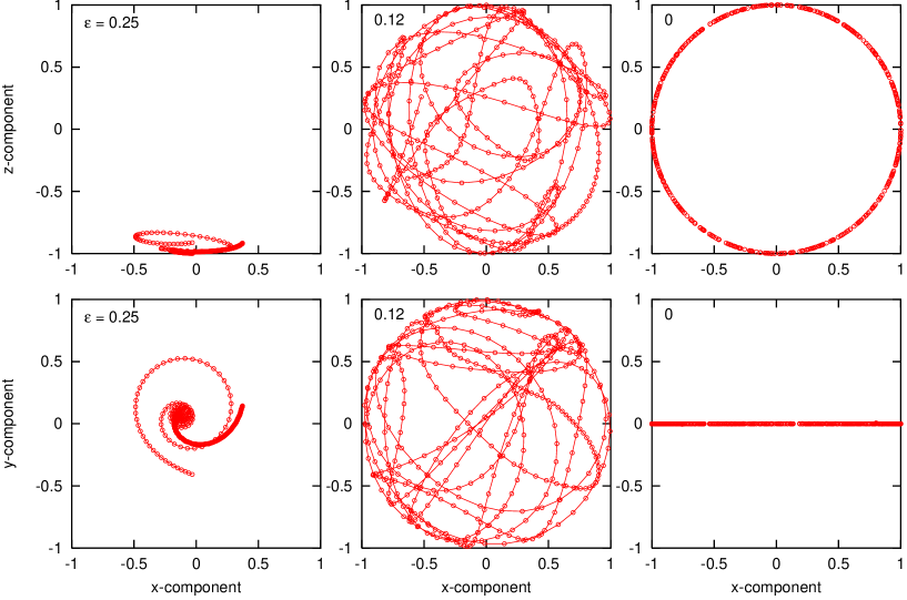
Figure 4.10: Final location on the unit sphere of 500 antineutrino polarization vectors for our standard parameters and the inverted hierarchy. The top row is the “side view” ($x$-$z$-components), the bottom row the “top view” ($x$-$y$-components). Left: quasi single-angle case ($\epsilon=0.25$). Middle: decoherent case ($\epsilon=0.12$). Right: symmetric system ($\epsilon=0$) [17].

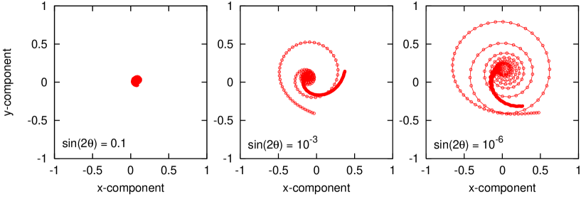
Figure 4.11: Same as Fig. 4.10, now only top views for quasi single-angle cases with the mixing angles $\sin 2\theta=0.1$, $10^{-3}$ and $10^{-6}$ from left to right. The middle panel is identical with the bottom left panel of Fig. 4.10 [17].

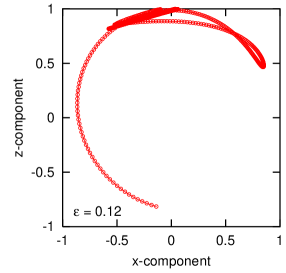
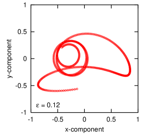
Figure 4.12: Same as Fig. 4.10, here for the normal hierarchy and $\epsilon=0.12$ [17].

Now turn to the quasi decoherent case with $\epsilon=0.12$. Initially the same happens, but at the “decoherence radius” the spiral structure dissolves almost instantaneously. The polarization vectors enter a complicated structure as illustrated by the end state (central panels of Fig. 4.10). Moreover, they are spread out all over the unit sphere, having both positive and negative $z$-components. This structure looks different for different choices of $\sin 2\theta$ and $\epsilon$. However, once a sufficient number of polarization vectors is used, it is reproducible. For $\epsilon=0.06$ the picture would be qualitatively similar.

Finally we show the fully symmetric case ($\epsilon=0$) in the right-hand panels. Here decoherence is fast and complete. For a small mixing angle, all polarization vectors are confined to the $x$-$z$-plane. They distribute themselves on a circle in that plane.

For the normal hierarchy, we show in Fig. 4.12 as an explicit example the $\epsilon=0.12$ case of Fig. 4.9 that showed a clear multi-angle effect without strong decoherence. Once more we find a spiral structure. Most polarization vectors remain oriented roughly in their original direction, but in this case also with a tail of a few polarization vectors reversed. The quasi decoherent case ($\epsilon=0.06$) and the symmetric system produce similar final pictures as the corresponding cases of the inverted hierarchy.
B) Measures of decoherence
Even in the quasi-decoherent cases the unit sphere is not uniformly filled with polarization vectors. Rather, in the mono-energetic case considered here, the occupied phase space is a one-dimensional subspace of the unit sphere. It is parameterized by the angular variable $u$ and shows a clear line-like structure. This picture suggests to use the length of this line on the unit sphere as another global measure besides the length $\bar{P}$ to discriminate between different modes of evolution [164]. In a numerical run with discrete angular bins, this quantity is simply the sum of the angles between neighboring polarization vectors. In Fig. 4.13 we show this quantity for the indicated values of $\epsilon$ as a function of radius for our inverted-hierarchy examples.

At the radius $r_{\rm syn}$ where the spiral forms, the length on the unit sphere quickly increases from 0 to a value that is almost independent of $\epsilon$, but depends on the mixing angle. For smaller $\sin 2\theta$ it is larger, corresponding to the spiral having more windings as indicated earlier. Later, this length stays practically constant, reflecting that the spiral structure, once established, does not change much except tilting toward the negative ${\bf B}$-direction and precessing around it.

When $\epsilon$ is smaller than a critical value, at the “decoherence radius” a sudden second growth shoots up from the plateau of these curves. For smaller $\epsilon$, the final length is longer, representing a more “phase-space filling” line on the unit sphere.

Note, however, that for $\epsilon$ close to zero, the line does not fill the unit sphere, but essentially stays in a narrow band. In the perfectly symmetric case, the motion of all polarization vectors is essentially confined to the $x$-$z$-plane, i.e., the polarization vectors distribute themselves over a great circle on the sphere as shown in the right panels of Fig. 4.10.

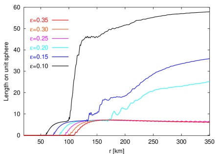
Figure 4.13: Evolution of the length of the one-dimensional subspace occupied by the polarization vectors for our standard inverted hierarchy case, taking a series of different asymmetries $\epsilon$. The length grows to larger values for smaller asymmetries [17].

4.3.3 Role of model parameters

A) Mixing angle
In the single-angle case, we have discussed that the mixing angle affects only to the onset of the bipolar conversions. This discussion suggests that, at least for the inverted hierarchy, the actual vacuum mixing angle does not strongly influence the issue of multi-angle decoherence because this effect happens when the global polarization vector is tilted far away from the ${\bf B}$ direction. On the other hand, we have already noted that the quasi-coherent spiral structure that forms just beyond the synchronization radius has more windings for a smaller mixing angle so that the system is not identical.

To clarify the role of the mixing angle we have used our standard inverted-hierarchy case and have calculated the limiting asymmetry $\epsilon$ for decoherence for a broad range of mixing angles. We show the limiting contours in the plane of $\epsilon$ and $\sin 2\theta$ in Fig. 4.14 for both hierarchies, above which multi-angle decoherence does not appear.

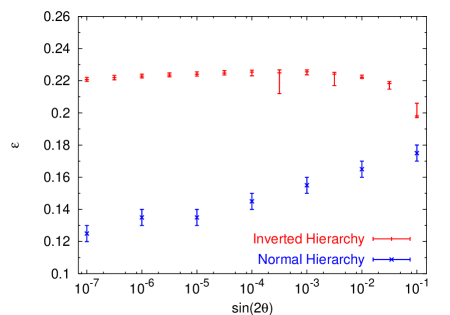
Figure 4.14: Limiting $\epsilon$ for decoherence as a function of mixing angle for our standard example and both hierarchies [17].

We emphasize that the limiting $\epsilon$ shown in Fig. 4.14 has a different meaning for the two hierarchies. As discussed earlier, in the inverted hierarchy, $\bar{P}$ shortens somewhat even in the quasi single-angle regime. Therefore, as a formal criterion for distinguishing the regions of coherence and decoherence we use that the final $\bar{P}$ has shortened to less than 0.85. The exact choice is irrelevant because the transition between the quasi-coherent and decoherent regimes is steep as a function of $\epsilon$.

Conversely, in the normal hierarchy, $\bar{P}$ need not visibly shorten at all as illustrated by the example in the lower left panel of Fig. 4.9. Therefore, we here demand that $\bar{P}$ does not visibly shorten in such a picture. We construct the demarcation line by decreasing $\epsilon$ in steps of 0.01 until the polarization vector for the first time shortens visibly. Finding this point requires a significant amount of manual iterations with a modified inner radius and number of angular bins to make sure the result does not depend on these numerical parameters. The error bars represent our confidence range for the true critical value.

We conclude that for the inverted hierarchy, multi-angle decoherence is virtually independent from the value of $\sin 2\theta$, except that for very large $\theta$ a slightly smaller asymmetry is enough to suppress decoherence. Assuming the presence of ordinary matter, such large mixing angles seem irrelevant, except perhaps at late times. Either way, it is conservative to assume a small mixing angle and we will use $\sin 2\theta=10^{-3}$ as a default value.

For the case of normal hierarchy we find a strong dependence of the critical $\epsilon$ on $\log_{10}(\sin 2\theta)$. For a smaller mixing angle it is easier to suppress decoherence. The normal hierarchy is very different from the inverted one in that for a small mixing angle, all polarization vectors stay closely aligned with the $z$-direction unless multi-angle decoherence takes place. Therefore, it is plausible that for a smaller mixing angle, decoherence effects are delayed.
B) Energy distribution
The neutrinos emitted from a SN core naturally have a broad energy distribution. In Ref. [164] it was noted that the energy distribution of neutrinos and antineutrinos is largely irrelevant for the question of decoherence as long as the oscillations exhibit self-maintained coherence [149]. The multi-angle transition to decoherence typically occurs within the dense-neutrino region where the synchronization of energy modes remains strong. Therefore, we expect that multi-angle decoherence is not significantly affected by the neutrino spectrum.

In order to compare a monochromatic system with one that has a broad energy distribution, the crucial quantity to keep fixed is not the average energy, but the average oscillation frequency $\langle\omega\rangle=\langle\Delta m^{2}/2E\rangle$, as discussed in Sec. 4.1.2. If we assume that neutrinos and antineutrinos have equal distributions, it is straightforward to adjust, for example, the temperature of a thermal distribution such that $\langle\omega\rangle$ is identical to our monochromatic standard case $\omega_{0}=0.3~{}{\rm km}^{-1}$. If we assume different distributions for neutrinos and antineutrinos, the equivalent $\omega_{0}$ is somewhat more subtle, and we will have to use Eq. (4.29).

We have studied several numerical examples of quasi single-angle behavior and of multi-angle decoherence, taking different neutrino and antineutrino energy spectra, such as flat or thermal and with equal or different temperatures. We always found that the evolution of the global polarization vectors is almost identical to the equivalent monochromatic cases. We never observed that a broad energy spectrum caused a significant deviation from the monochromatic behavior at those radii that are relevant for decoherence.

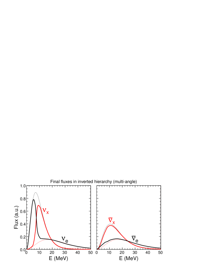
Figure 4.15: Multi-angle simulation in inverted hierarchy: Final fluxes after the bipolar conversions for different neutrino species as a function of energy. Initial fluxes are shown as dotted lines to guide the eye [16].

Of course, a multi-energy system is qualitatively different from a monochromatic one in that the final energy distribution shows a spectral split. Nevertheless, for sufficiently large asymmetries $\epsilon$ where the multi-angle system evolves in the quasi single-angle mode, there is no significant modification of the spectral split. In Ref. [16] it is performed this analysis for a fixed value of the $\epsilon$. They indeed obtain the same kind of spectral split as in the single-angle case. Their result is shown in Fig. 4.15. In the decoherent case, on the other hand, the final spectra naturally are very different, but we have not explored such cases systematically because multi-angle decoherence does not seem to be generic for realistic SN scenarios.

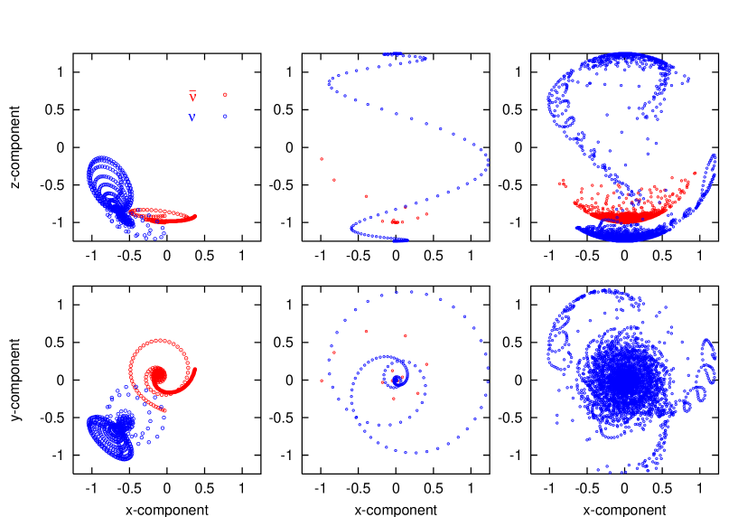
Figure 4.16: Final state at a large radius of the polarization vectors for our standard parameters in analogy to Fig. 4.10. The antineutrinos (red/light gray) are on the unit sphere, whereas the neutrinos (blue/dark gray) live on a sphere of radius $1+\epsilon=1.25$. Left: monochromatic multi-angle, the antineutrinos being identical with the left column of Fig. 4.10. Middle: Box-like energy spectrum and single angle. Right: Box-like energy spectrum and multi angle. In the lower right panel we do not show the antineutrinos [17].

To illustrate the modifications caused by an energy spectrum in a different way from the previous literature, we show in Fig. 4.16 the side and top views of the location of neutrino and antineutrino polarization vectors on the unit sphere in analogy to Fig. 4.10 for our standard parameter values. In the left column we show the same monochromatic multi-angle case that we already showed in the left column of Fig. 4.10, with 500 modes. In addition we include the neutrinos (blue/dark gray) that here live on a sphere of radius $1+\epsilon=1.25$. The neutrinos form a spiral structure similar to the one of the antineutrinos, but in the final state this structure cannot move to the negative ${\bf B}$ directions because of lepton number conservation.

In the middle column we show a single-angle example with the same parameters, now using a box-like spectrum of oscillation frequencies where initially $\bar{P}_{\omega}^{z}=(2\omega_{0})^{-1}$ and $P_{\omega}^{z}=(1+\epsilon)(2\omega_{0})^{-1}$ for $0\leq\omega\leq 2\omega_{0}$ so that $\langle\omega_{\nu}\rangle=\langle\omega_{\bar{\nu}}\rangle=\omega_{0}$ and it is equivalent to the original monochromatic case. We now see that most of the antineutrinos have moved to the negative ${\bf B}$ direction as before, whereas the neutrinos populate both the positive and negative ${\bf B}$ direction, representing the spectral split. The lack of full adiabaticity prevents the split from being complete, leaving some polarization vectors not fully aligned or anti-aligned with ${\bf B}$. At large radii when the neutrino-neutrino interactions have died out, these modes precess with their different vacuum oscillation frequencies so that they are found on a spiral locus extending from the “south pole” to the “north pole” that gets wound up further at larger radii. Note that here we have used 1000 energy modes in order to obtain a visible population occupying these non-adiabatic final states. Still, only very few red dots (antineutrinos) are visible, the vast majority being at the south pole. Likewise for the neutrinos (blue dots), the spiral is populated only by a small fraction of the 1000 modes. In other words, the evolution is nearly adiabatic.

Finally we combine a box-like energy spectrum and a multi-angle distribution (right panels). The antineutrinos all cluster around the negative ${\bf B}$ direction and fill the “southern polar cap” more or less uniformly because at late times modes with different energies precess with different frequencies. The neutrinos populate both the northern and southern polar caps, representing the spectral split. At intermediate latitudes we find coherent spiral structures. They correspond to modes with different angles but equal $\omega$ so that even at late times they do not dissolve by differential precession.
C) Effective interaction strength
Besides the asymmetry $\epsilon$ itself, the most uncertain model parameter is the effective neutrino-neutrino interaction strength $\mu_{0}$ as defined in Eq. (4.7). In Fig. 4.17 we show the demarcation lines between coherence and decoherence for both hierarchies in the $\mu_{0}$-$\epsilon$-plane, keeping all other parameters at their standard values. The contours are constructed as described in the discussion for the mixing angle at the beginning of this section. The numerical contours are visually very well approximated by linear regressions of the form

$$\epsilon_{\rm IH} \approx 0.225+0.027\,\log_{10}\left(\frac{\mu_{0}}{10^{6}~{}{\rm km}^{-1}}\right)\,,$$

$$\epsilon_{\rm NH} \approx 0.172+0.087\,\log_{10}\left(\frac{\mu_{0}}{10^{6}~{}{\rm km}^{-1}}\right)\,.$$ (4.45)

For the normal hierarchy, the linear regression would intersect $\epsilon=0$ within the range of investigated $\mu_{0}$-values, but in reality turns over and saturates around $\epsilon=0.06$.
D) Vacuum oscillation frequency
The average vacuum oscillation frequency $\omega$ depends on the atmospheric $\Delta m^{2}$ that is quite well constrained, and a certain average of the neutrino energies. Our standard value is $\omega=0.3~{}{\rm km}^{-1}$. If we increase this to $1~{}{\rm km}^{-1}$, the $\epsilon$-$\mu_{0}$-contour in Fig. 4.17 is essentially parallel-shifted to larger $\epsilon$ by about 0.035 (inverted hierarchy). This range of $\omega$ probably brackets the plausible possibilities so that the uncertainty of $\omega$ does not strongly influence the practical demarcation between the regimes.

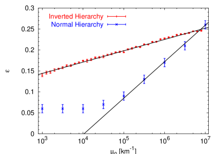
Figure 4.17: Limiting $\epsilon$ for decoherence as a function of the effective neutrino-neutrino interaction strength $\mu_{0}$ for our standard parameters. The linear regressions are “visual fits” represented by Eq. (4.3.3) [17].

The normal hierarchy is more sensitive to $\omega$. In Fig. 4.18 we show a contour for the coherence regime in the $\epsilon$-$\omega$ plane, assuming otherwise our standard parameter values. Changing $\omega$ from $0.3$ to $1~{}{\rm km}^{-1}$ increases the critical $\epsilon$ by almost 0.15.

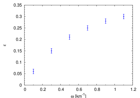
Figure 4.18: Limiting $\epsilon$ for decoherence as a function of the vacuum oscillation frequency $\omega$ for our standard parameters and the normal hierarchy [17].

4.3.4 Concluding remarks

We have here not attempted to develop further analytical insights, but have taken a practical approach and explored numerically the range of parameters where different forms of behavior dominate in a realistic SN scenario.

To this end we have first clarified that “multi-angle effects” means one of two clearly separated forms of behavior. The flavor content of the system can evolve in a quasi single-angle form. On the level of the polarization vectors this means that they fill only a restricted volume of the available phase space and maintain a coherent structure. On the other hand, nearly complete flavor equilibrium can arise where the available phase space is more or less uniformly filled.

For realistic assumptions about SN and neutrino parameters, the switch between these modes of evolution is set by the degree of asymmetry between the neutrino and antineutrino fluxes. While this asymmetry is caused by the deleptonization flux, the crucial parameter $\epsilon$ is the asymmetry between $F^{R_{\nu}}_{\nu_{e}}-F^{R_{\nu}}_{\nu_{x}}$ and the corresponding antineutrino quantity as defined in Eq. (4.11) because for flavor oscillations the part of the density matrix that is proportional to $F^{R_{\nu}}_{\nu_{e}}+F^{R_{\nu}}_{\nu_{x}}$ drops out. While in a realistic SN on average $F^{R_{\nu}}_{\nu_{e}}$ is about 15% larger than $F^{R_{\nu}}_{\bar{\nu}_{e}}$, the asymmetry parameter as defined in Eq. (4.11) is typically much larger.

The critical value of $\epsilon$ that is enough to suppress decoherence depends on the type of neutrino mass hierarchy, the average energies, luminosities, and on the mixing angle. We have found that for $\epsilon>0.3$, decoherence is suppressed for the entire range of plausible parameters, but a value smaller than 0.1 may be enough, depending on the combination of other parameters.

We conclude that the quasi single-angle behavior may well be typical for realistic SN conditions, i.e., that the deleptonization flux is enough to suppress multi-angle decoherence. To substantiate this conclusion one should analyze the output of numerical simulations in terms of our model parameters. Besides the flavor-dependent luminosities and average energies, one needs the angular distribution of the neutrino radiation field at some radius where collisions are no longer important.

If our conclusion holds up in the light of realistic SN simulations, a practical understanding of the effect of self-induced neutrino flavor transformations quickly comes into reach. In the normal mass hierarchy, nothing new would happen on a macroscopic scale. In the inverted hierarchy, the final effect would be a conversion of $\nu_{e}\bar{\nu}_{e}$ pairs and a split in the $\nu_{e}$ spectrum. These phenomena are only mildly affected by multi-angle effects as long as we are in the quasi single-angle regime.

If at late times the matter density profile contracts enough that an MSW effect occurs in the dense-neutrino region, the situation becomes more complicated as the neutrino-neutrino and ordinary matter effects interfere and produce a richer structure of spectral modifications [160, 161]. Even then, numerical simulations are much simpler if multi-angle decoherence is suppressed.

It is not obvious how $\epsilon$ evolves at late times. The deleptonization of the core is probably faster than the cooling so that one may think that $\epsilon$ becomes smaller. On the other hand, the $\bar{\nu}_{e}$ can essentially only interact via neutral current reactions and their flux and energy distribution should, therefore, become very similar to the ones of $\nu_{x}$ and $\bar{\nu}_{x}$. Therefore, it is not obvious if at late times the initial flux difference $F^{R_{\nu}}_{\nu_{e}}-F^{R_{\nu}}_{\bar{\nu}_{e}}$ or $F^{R_{\nu}}_{\bar{\nu}_{e}}-F^{R_{\nu}}_{\bar{\nu}_{x}}$ decreases more quickly. We also note that there can be a cross-over in the sense that at late times the flux hierarchy can become $F^{R_{\nu}}_{\nu_{x}}=F^{R_{\nu}}_{\bar{\nu}_{x}}>F^{R_{\nu}}_{\nu_{e}}>F^{R_{\nu}}_{\bar{\nu}_{e}}$ as in Ref. [178], meaning that we would have a pair excess flux of $\nu_{x}\bar{\nu}_{x}$ instead of a $\nu_{e}\bar{\nu}_{e}$ excess.

Our results suggest that signatures of collective flavor transformations are not erased by multi-angle decoherence and will survive to the surface, modulated by the usual MSW flavor conversions [179]. The survival of observable signatures then also depends on the density fluctuations of the ordinary medium that can be a source of kinematical flavor decoherence [180, 181].

All authors in this field have relied on the simplifying assumption of either homogeneity or exact spherical symmetry to make the equations numerically tractable. The neutrino emission from a real SN is influenced by density and temperature fluctuations of the medium in the region where neutrinos decouple. Likewise, the neutrino fluxes emitted from the accretion tori of coalescing neutron stars, the likely engines of short gamma ray bursts, have fewer symmetries than assumed here. It remains to be investigated if systems with more general geometries behave qualitatively similar to the spherically symmetric case or if deviations from spherical symmetry can provide a new source of kinematical decoherence.

4.4 Role of dense matter in collective supernova neutrino transformations

Let us now analyze the other potential source of multi-angle decoherence in the collective neutrino transformations, namely the dense matter background. One of the many surprises of self-induced flavor transformations has been that, in the single-angle approximation, dense matter barely affects them. They are driven by an instability in flavor space that is insensitive to matter because it affects all neutrino and antineutrino modes in the same way. Therefore, it can be transformed away by going to a rotating frame in flavor space, see Eq. (4.10).

We here clarify, however, that the matter density can not be arbitrarily large before it affects collective flavor conversions after all. The matter term is “achromatic” only if we consider the time–evolution of a homogeneous (but not necessarily isotropic) neutrino ensemble on a homogeneous and isotropic matter background. If the matter background is not isotropic, the current-current nature of the neutrino-electron interaction already implies that different neutrino modes experience a different matter effect.

It is more subtle that even without a current, matter still affects different neutrino modes differently if we study neutrinos streaming from a source. The relevant evolution is now the flavor variation of a stationary neutrino flux as a function of distance. For a spherically symmetric situation, “distance from the source” is uniquely given by the radial coordinate $r$. Neutrinos reaching a certain $r$ have travelled different distances on their trajectories if they were emitted with different angles relative to the radial direction. Therefore, at $r$ they have accrued different oscillation phases even if they have the same vacuum oscillation frequency and even if they have experienced the same matter background. In other words, if we project the flavor evolution of different angular modes on the radial direction, they have different effective vacuum oscillation frequencies even if they have the same energy. The same argument applies to matter that modifies the oscillation frequency in the same way along each trajectory, but therefore acts differently when expressed as an effective oscillation frequency along the radial direction.

The neutrino-neutrino interaction, when it is sufficiently strong, forces different modes to reach a certain $r$ with the same oscillation phase. To achieve this “self-maintained coherence” the neutrino-neutrino term must overcome the phase dispersion that would otherwise occur. Such a dispersion is caused not only by a spectrum of energies, but also by a matter background.

4.4.1 Homogeneous Ensemble

A) Isotropic background
Let us reanalyze the role of matter in collective neutrino transformations. We begin with the EOMs in their simplest form, relevant for a homogeneous (but not necessarily isotropic) gas of neutrinos. We only consider two-flavor oscillations where the most economical way to write the EOMs is in terms of the usual flavor polarization vectors ${\bf P}_{\bf p}$ for each mode ${\bf p}$ and analogous vectors $\bar{\bf P}_{\bf p}$ for the antineutrinos, as shown in Eq. (4.5). For simplicity we here assume that initially only $\nu_{e}$ and $\bar{\nu}_{e}$ are present with an excess neutrino density of $n_{\nu_{e}}=(1+\epsilon)\,n_{\bar{\nu}_{e}}$. The polarization vectors are initially normalized such that $|\int{\rm d}{\bf p}\,\bar{\bf P}_{\bf p}|=1$ and $|\int{\rm d}{\bf p}\,{\bf P}_{\bf p}|=1+\epsilon$.

The matter term is “achromatic” in that it affects all modes of neutrinos and antineutrinos in the same way. As already discussed, one may study the EOMs in a coordinate system that rotates around ${\bf L}$ with frequency $\lambda$ so that the matter term disappears. In the new frame the vector ${\bf B}$ rotates fast around ${\bf L}$ so that its transverse component averages to zero. Therefore, in the new frame the rotation-averaged Hamiltonian is

$$\langle{\bf H}\rangle=\omega\cos(2\theta)\,{\bf L}+\mu({\bf P}-\bar{\bf P})\,,$$ (4.46)

where for the moment we consider the even simpler case of an isotropic and monochromatic neutrino ensemble where the entire system is described by one polarization vector ${\bf P}$ for neutrinos and one $\bar{\bf P}$ for antineutrinos.

A dense matter background effectively projects the EOMs on the weak-interaction direction. In particular, the relevant vacuum oscillation frequency is now $\omega\cos 2\theta$. For a small mixing angle, the case usually considered in this context, this projection effect is not important. However, a large mixing angle would strongly modify the projected $\omega$. Maximal mixing where $\cos 2\theta=0$ would prevent any collective flavor transformations, an effect that is easily verified in numerical examples.

One usually assumes that the (anti)neutrinos are prepared in interaction eigenstates so that initially ${\bf P}$ and $\bar{\bf P}$ are oriented along ${\bf L}$. Therefore, the rotation-averaged EOMs alone do not lead to an evolution. However, in the unstable case of the inverted mass hierarchy, an infinitesimal disturbance is enough to excite the transformation. The fast-rotating transverse ${\bf B}$ component that was left out from the EOM is enough to trigger the evolution, but otherwise plays no crucial role [159, 14].

If we consider a homogeneous system where $\mu$ is a slowly decreasing function of time, one can find the adiabatic solution of the EOM for the simple system consisting only of ${\bf P}$ and $\bar{\bf P}$ [163, 165]. In vacuum, this is a complicated function of $\epsilon$ and $\cos 2\theta$. In dense matter, however, we are effectively in the limit of a vanishing mixing angle because the initial orientation of the polarization vectors now coincides with the direction relevant for the rotation-averaged evolution. The original vacuum mixing angle only appears in the expression for the projected oscillation frequency $\omega\cos 2\theta$.

With $z=\bar{P}_{z}$ the adiabatic connection between $\bar{P}_{z}$ and $\mu$ is now given by the inverse function of

$$\frac{\omega\cos 2\theta}{\mu}=\frac{\epsilon+2z}{2}-\frac{\epsilon+2z+(3\epsilon+2z)z}{2\sqrt{(1+z)(1+z+2\epsilon)}}\,,$$ (4.47)

where $-1\leq z\leq+1$. The synchronization radius $r_{\rm syn}$ where the adiabatic curve begins its decrease is implied by $\bar{P}_{z}=z=1$. One finds the familiar result of Eq. (4.12)

$$\frac{\omega\cos 2\theta}{\mu}\Big{|}_{\rm syn}=\frac{(\sqrt{1+\epsilon}-1)^{2}}{2}\,.$$ (4.48)

For $\mu$ values larger than this limit, the polarization vectors are stuck to the ${\bf L}$ direction.

Without matter one finds that $({\bf P}-\bar{\bf P})\cdot{\bf B}$ is conserved. Here, the analogous conservation law applies to $({\bf P}-\bar{\bf P})\cdot{\bf L}$. Therefore, the adiabatic solution for $P_{z}$ is such that $P_{z}-\bar{P}_{z}$ is conserved, i.e., $P_{z}=\bar{P}_{z}+\epsilon$.

In summary, the presence of dense matter simplifies the EOMs and in that the adiabatic solution is the one for a vanishing vacuum mixing angle, provided one uses the projected vacuum oscillation frequency.
B) Background flux
As a next example we still consider a homogeneous system, but now allow for a net flux of the background matter, assuming axial symmetry around the direction defined by the flux. For simplicity we consider a monochromatic ensemble with a single vacuum oscillation frequency $\omega$. We characterize the angular neutrino modes by their velocity component $v$ along the matter flux direction. The EOMs are in this case

$$\dot{\bf P}_{v}={\bf H}_{v}\times{\bf P}_{v}\,.$$ (4.49)

The Hamiltonian for the mode $v$ is

$${\bf H}_{v}=\omega{\bf B}+(\lambda-\lambda^{\prime}v){\bf L}+\mu({\bf D}-v{\bf F})\,,$$ (4.50)

where $\lambda^{\prime}\equiv\lambda v_{e}$, $v_{e}$ being the net electron velocity. Moreover,

$${\bf D} = \int_{-1}^{+1}{\rm d}v\,\left({\bf P}_{v}-\bar{\bf P}_{v}\right)\,,$$

$${\bf F} = \int_{-1}^{+1}{\rm d}v\,v\left({\bf P}_{v}-\bar{\bf P}_{v}\right)$$ (4.51)

are the net neutrino density and flux polarization vectors. The normalization is $|\int{\rm d}v\,\bar{\bf P}_{v}|=1$ and $|\int{\rm d}v\,{\bf P}_{v}|=1+\epsilon$.

Next, we transform the EOMs to a frame rotating with frequency $\lambda$, allowing us to remove the matter term, but not the matter flux,

$$\langle{\bf H}_{v}\rangle=(\omega-\lambda^{\prime}v){\bf L}+\mu({\bf D}-v{\bf F})\,.$$ (4.52)

We assume $\theta$ to be small and thus use $\omega\approx\omega\cos 2\theta$. We now have a system where the effective vacuum oscillation frequencies for neutrinos are uniformly distributed between $\omega\pm\lambda^{\prime}$ and for antineutrinos between $-\omega\pm\lambda^{\prime}$. Even after removing the average common precession of all modes, their evolution is still dominated by the matter-flux term if $\lambda^{\prime}\gg\mu$. In other words, collective behavior now requires $\mu>\lambda^{\prime}$ and not only $\mu>\omega$.

The simplest example is the flavor pendulum where for $\epsilon=0$ and an isotropic neutrino gas one obtains the well-known pendular motions of the polarization vectors. Matter does not disturb this behavior, except that it takes logarithmically longer for the motion to start. However, a matter flux, if sufficiently strong, suppresses this motion and the polarization vectors remain stuck to the ${\bf L}$ direction for both mass hierarchies. If the neutrino distribution is not isotropic, the ensemble quickly decoheres kinematically [164], an effect that is also suppressed by a sufficiently strong matter flux.

We have verified these predictions in several numerical examples, but have not explored systematically the transition between a “weak” and a “strong” matter flux because a homogeneous ensemble only serves as a conceptual example where matter can have a strong influence on self-induced transformations.

4.4.2 Spherical Stream

The most general case of neutrino flavor evolution consists of an ensemble evolving both in space and time. In practice, however, one usually considers quasi-stationary situations where one asks for the spatial flavor variation of a stationary neutrino flux streaming from a source. The neutrino density decreases with distance so that one can mimic this situation by a homogeneous system evolving in time with a decreasing density, the expanding universe being a realistic example. However, the analogy has important limitations because collective oscillations introduce geometric complications into the spatial-variation case.

The simplest non-trivial example is a perfectly spherical source (“SN core”) that emits neutrinos and antineutrinos like a blackbody surface into space. The matter background is also taken to be perfectly spherically symmetric, but of course varies with radius. As a further simplification we consider monochromatic neutrinos and antineutrinos that are all emitted with the same energy. In such a system, we end up with the EOMs given in Eq. (4.2), which we can rewrite as

$$\partial_{r}{\bf P}_{u}={\bf H}_{u}\times{\bf P}_{u}\,,$$ (4.53)

where the Hamiltonian is

$${\bf H}_{u}=\frac{\omega{\bf B}+\lambda{\bf L}}{v_{u}}+\mu_{r}\left(\frac{{\bf D}}{v_{u}}-{\bf F}\right)\,.$$ (4.54)

For antineutrinos we have, as always, $\omega\to-\omega$. Since the polarization vectors describe the fluxes, the global density and flux polarization vectors are

$${\bf D} = \int_{0}^{1}{\rm d}u\,\frac{{\bf P}_{u}-\bar{\bf P}_{u}}{v_{u}}\,,$$

$${\bf F} = \int_{0}^{1}{\rm d}u\,\left({\bf P}_{u}-\bar{\bf P}_{u}\right)\,,$$ (4.55)

using the normalization $|\int_{0}^{1}{\rm d}u\,\bar{\bf P}_{u}|=1$ and $|\int_{0}^{1}{\rm d}u\,{\bf P}_{u}|=1+\epsilon$. The matter coefficient $\lambda=\sqrt{2}\,G_{\rm F}[n_{e^{-}}(r)-n_{e^{+}}(r)]$ encodes the effective electron density at radius $r$ whereas

$$\mu_{r}=\mu_{0}\,\frac{R_{\nu}^{2}}{r^{2}}\,.$$ (4.56)

Therefore, $\mu_{r}$ always varies as $r^{-2}$ due to the geometric flux dilution, whereas $\lambda$ is given by the detailed matter profile of a SN model [70, 71, 66].

The variation of the polarization vectors with the common radial coordinate $r$ now acquires dynamical significance in that the polarization vectors evolve differently than they would in the absence of neutrino-neutrino interactions. From Eq. (4.54) it is obvious that the matter term is no longer the same for all modes and thus can not be transformed away by going to a rotating frame. This behavior does not depend on the radial variation of $\lambda$, even a homogeneous medium would show this multi-angle matter effect.

For quasi single-angle behavior to occur, $\epsilon$ must not be too small, a condition that is probably satisfied in a realistic SN. Therefore, the synchronization radius implied by Eq. (4.48) is always much larger than the neutrino-sphere radius $R_{\nu}$, allowing us to expand the EOMs in powers of $R_{\nu}/r\ll 1$. Using

$$v_{u}^{-1}=1+\frac{u}{2}\,\frac{R_{\nu}^{2}}{r^{2}}$$ (4.57)

we find

$${\bf H}_{u}=(\omega{\bf B}+\lambda{\bf L})\left(1+\frac{u}{2}\,\frac{R_{\nu}^{2}}{r^{2}}\right)+\mu_{r}\,\frac{R_{\nu}^{2}}{2r^{2}}\left({\bf Q}+u{\bf F}\right)\,,$$ (4.58)

where

$${\bf Q}=\int_{0}^{1}{\rm d}u\,u\left({\bf P}_{u}-\bar{\bf P}_{u}\right)$$ (4.59)

and ${\bf F}$ is the same as before. At large $r$ a small correction to $\omega$ is not crucial and can be ignored. The radial variation of $\lambda$ is slow compared to the precession, so we can go to a frame that rotates with a different frequency $\lambda$ at each radius. Finally the rotation-averaged Hamiltonian is

$$\langle{\bf H}_{u}\rangle=(\omega+u\,\lambda^{*})\,{\bf L}+\mu^{*}\,\left({\bf Q}+u{\bf F}\right)\,,$$ (4.60)

where we have assumed $\omega\cos 2\theta\approx\omega$ and defined

$$\lambda^{*} = \lambda\,\frac{R_{\nu}^{2}}{2r^{2}}\,,$$

$$\mu^{*} = \mu_{r}\,\frac{R_{\nu}^{2}}{2r^{2}}=\mu_{0}\,\frac{R_{\nu}^{4}}{2r^{4}}\,.$$ (4.61)

The multi-angle matter effect can be neglected if in the collective region beyond the synchronization radius we have

$$\lambda^{*}\ll\mu^{*}$$ (4.62)

equivalent to

$$n_{e^{-}}-n_{e^{+}}\ll n_{\bar{\nu}_{e}}\,.$$ (4.63)

In the opposite limit we expect that the large spread of effective oscillation frequencies prevents collective oscillations. In this case all polarization vectors remain pinned to the ${\bf L}$ direction and no flavor conversion occurs.

For intermediate values it is not obvious what will happen. One may expect that the multi-angle matter effect triggers multi-angle decoherence, destroying the quasi single-angle behavior. This indeed occurs for the inverted hierarchy whereas in the normal hierarchy we have not found any conditions where multi-angle decoherence was triggered by the multi-angle matter effect. We recall that for a sufficiently small $\epsilon$ multi-angle decoherence occurs even in the normal hierarchy whereas no collective transformation arise for a sufficiently large $\epsilon$ [17].

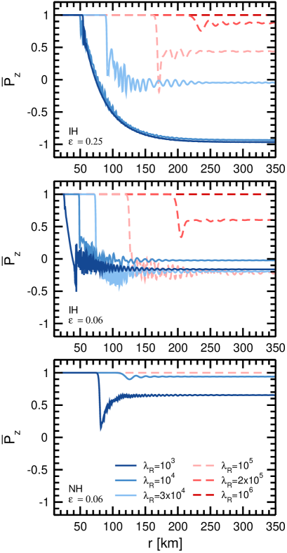
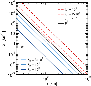
Figure 4.19: On the left plot we show the radial variation of $\mu^{*}$ and $\lambda^{*}$ for our numerical examples with the indicated value of $\lambda_{R}\equiv\lambda_{R_{\nu}}$. On the right plots we have the radial variation of $\bar{P}_{z}$ for three different scenarios: IH and $\epsilon=0.25$ (top panel), IH and $\epsilon=0.06$ (middle panel), and NH and $\epsilon=0.06$ (bottom panel). In each panel different values of $\lambda_{R_{\nu}}$ have been assumed [20].

We illustrate these points with a numerical example where $R_{\nu}=10$ km, $\omega=0.3~{}{\rm km}^{-1}$, $\theta=10^{-2}$, $\mu_{0}=7\times 10^{4}~{}{\rm km}^{-1}$ and

$$\lambda=\lambda_{R_{\nu}}\,\left(\frac{R_{\nu}}{r}\right)^{n}$$ (4.64)

with $n=2$. This particular value of the power-law index leads to the same radial dependence of $\mu^{*}$ and $\lambda^{*}$, see Eq. (4.4.2). In the left plot of Fig. 4.19 we show the radial variation $\mu^{*}$ and $\lambda^{*}$ for different choices of $\lambda_{R_{\nu}}$, between $10^{3}$ km^-1 and $10^{6}$ km^-1. Even for the smallest matter effect, the ordinary MSW resonance, defined by the condition $\lambda=\omega$, stays safely beyond the collective region.

In the right plots of Fig. 4.19 we show the corresponding variation of $\bar{P}_{z}$ for three different cases: inverted mass hierarchy and $\epsilon=0.25$ (top panel), inverted mass hierarchy and $\epsilon=0.06$ (middle panel), and normal mass hierarchy and $\epsilon=0.06$ (bottom panel). In the top panel we observe the usual transformation for a small matter effect, a complete suppression of transformations for a large matter effect, and multi-angle decoherence for intermediate cases. Repeating the same exercise for the normal mass hierarchy and the same $\epsilon$ reveals no macroscopic influence of the matter term.

For a sufficiently small $\epsilon$ one finds self-induced multi-angle decoherence for both hierarchies. In the middle and bottom panels of Fig. 4.19 we show how with a sufficiently strong matter effect the decoherence can be suppressed for both hierarchies.

4.4.3 Discussion

We have identified a new multi-angle effect in collective neutrino transformations that is caused by a matter background. Previous numerical studies of multi-angle effects had used a matter profile that satisfies the condition Eq. (4.63) in the critical region [160, 16]. In other multi-angle studies matter was entirely ignored [17] and otherwise, single-angle studies were performed. Therefore, the multi-angle matter effect discussed here had escaped numerical detection.

In many practical cases relevant for SN physics or in coalescing neutron stars, the density of matter is probably small enough so that this effect can be ignored. On the other hand, for iron-core SNe, during the accretion phase the matter can be large enough to be important.

If at early times the matter density profile is such that our multi-angle effect is important, this will not be the case at later times when the explosion has occurred and the matter profile contracts toward the neutron star. In principle, therefore, interesting time-dependent features in the oscillation probability can occur.

A large matter effect can be “rotated away” from the EOMs when it is identical for all modes. Here we have seen that even a perfectly uniform medium provides a multi-angle variation of the matter effect. We note that the matter fluxes would not be important, in contrast to our first example of a homogeneous ensemble, because the relevant quantity is the spread of the matter effect between different modes. Therefore, whenever a flux term would be important, the matter density term already provides a strong multi-angle effect.

In addition, the medium can have density variations caused by convection and turbulence [182] that is known to affect the MSW resonance under certain circumstances [183, 180, 181, 184, 185]. Density variations in the transverse direction to the neutrino stream lines may well cause important variations of the matter effect between different modes. It remains to be investigated in which way collective flavor transformations are affected.

Chapter 5 Collective Supernova Neutrino Transformations in Three Flavors

We here extend our previous numerical analysis to the case of three neutrino flavors. Our main results can be summarized as follows: (i) A two-flavor treatment indeed captures the full effect if one ignores the mu-tau potential, $V_{\mu\tau}$, and if the ordinary MSW resonances occur outside of the collective neutrino region. (ii) Including $V_{\mu\tau}$ can strongly modify the $\nu_{e}$ or $\bar{\nu}_{e}$ survival probabilities, influencing the neutrino signal from the next galactic SN. (iii) The effect depends sensitively on a possible deviation from maximal $\theta_{23}$. (iv) The inclusion of $V_{\mu\tau}$ also affects the onset of the bipolar conversions. (v) Multi-angle matter decoherence possibly supresses these effects.

5.1 Introduction

As it was discussed in Chapter 2, neutrinos of different flavor suffer different refraction in matter. The energy shift between $\nu_{e}$ and $\nu_{\mu}$ or $\nu_{\tau}$ is $V_{\rm CC}=\sqrt{2}\,G_{\rm F}Y_{e}n_{B}$ with $G_{\rm F}$ the Fermi constant, $n_{B}$ the baryon density, and $Y_{e}=n_{e}/n_{B}$ the electron fraction. The potential $V_{\rm CC}$ is caused by the charged-current $\nu_{e}$-electron interaction that is absent for $\nu_{\mu}$ and $\nu_{\tau}$. For a matter density $\rho=1$ g cm^-3 we have $\sqrt{2}\,G_{\rm F}n_{B}=7.6\times 10^{-14}$ eV, yet this small energy shift is large enough to be of almost universal importance for neutrino oscillation physics.

In normal matter, $\mu$ and $\tau$ leptons appear only as virtual states in radiative corrections to neutral-current $\nu_{\mu}$ and $\nu_{\tau}$ scattering, causing a shift $V_{\mu\tau}=\sqrt{2}\,G_{\rm F}Y_{\tau}^{\rm eff}n_{B}$ between $\nu_{\mu}$ and $\nu_{\tau}$. It has the same effect on neutrino dispersion as real $\tau$ leptons with an abundance [61]

$$Y_{\tau}^{\rm eff}=\frac{3\sqrt{2}\,G_{\rm F}m_{\tau}^{2}}{(2\pi)^{2}}\left[\ln\left(\frac{m_{W}^{2}}{m_{\tau}^{2}}\right)-1+\frac{Y_{n}}{3}\right]=2.7\times 10^{-5}\,,$$ (5.1)

as defined in Eq. (2.34), where $n_{e}=n_{p}$ was assumed. For the neutron abundance we have used $Y_{n}=n_{n}/n_{B}=0.5$, but it provides only a 2.5% correction so that its exact value is irrelevant. As discussed in Chapter 3, a large non-standard contribution to $Y_{\tau}^{\rm eff}$ can arise from radiative corrections in supersymmetric models [186], but we will focus in this chapter on the standard-model effect alone.

This “mu–tau matter effect” modifies oscillations if $V_{\mu\tau}>\Delta m^{2}/2E$. For propagation through the Earth and for $\Delta m^{2}_{\rm atm}=2$–$3\times 10^{-3}~{}{\rm eV}^{2}$, this occurs for neutrino energies $E>100$ TeV. The oscillation length then far exceeds $r_{\rm Earth}$ so that $V_{\mu\tau}$ is irrelevant for the high-energy neutrinos that are searched for by neutrino telescopes.

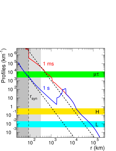
Figure 5.1: Density profiles in terms of the weak potential $V_{\rm CC}=\sqrt{2}\,G_{\rm F}n_{e}$ at 1 ms and 1 s post bounce of the numerical SN models described in Ref. [177] (solid lines). The dashed lines represent the simplified matter profile of Eq. (5.4) for $\lambda_{0}=4\times 10^{6}$ km^-1 and $\lambda_{0}=5\times 10^{9}$ km^-1, used in our numerical calculations in Figure 5.2. As horizontal bands we indicate the conditions $V_{\mu\tau}=\Delta m^{2}_{\rm atm}/2E$, $V_{\rm CC}=\Delta m^{2}_{\rm atm}/2E$, and $V_{\rm CC}=\Delta m^{2}_{\rm sol}/2E$ for a typical range of SN neutrino energies. The gray shaded range of radii corresponds to the region of collective neutrino transformations. Within the radius $r_{\rm syn}$ the collective oscillations are of the synchronized type [18].

Alternatively, the mu–tau matter effect can be important at the large densities encountered by neutrinos streaming off a SN core [75]. For $E=20~{}{\rm MeV}$ the condition $V_{\mu\tau}=\Delta m^{2}_{\rm atm}/2E$ implies $\rho\approx 3\times 10^{7}~{}{\rm g}~{}{\rm cm}^{-3}$. Numerical SN density profiles [177] reveal that this occurs far beyond the shock-wave radius during the accretion phase, but retracts close to the neutrino sphere after the explosion has begun. To illustrate this point we show in Fig. 5.1 the same matter density profiles as in Ref. [177] at 1 ms post bounce (red line) and at 1 s post bounce (blue line). As a green horizontal band we indicate the condition $V_{\mu\tau}=\Delta m^{2}_{\rm atm}/2E$ for a typical range of SN neutrino energies, whereas the yellow and light-blue bands indicate the densities corresponding to the $H$-resonance (driven by $\Delta m_{\rm atm}^{2}$) and the $L$-resonance (driven by $\Delta m_{\rm sol}^{2}$). The $\nu_{\mu}$, $\nu_{\tau}$, $\bar{\nu}_{\mu}$ and $\bar{\nu}_{\tau}$ fluxes from a SN are virtually identical, leaving the $\mu\tau$-resonance moot, whereas the $H$- and $L$-resonances cause well-understood consequences that are completely described by the energy-dependent swapping probabilities for $\nu_{e}$ and $\bar{\nu}_{e}$ with some combination $\nu_{x}$ of the $\mu$ and $\tau$ flavor [179], as discussed in Chapter 2. Therefore, the traditional view has been that genuine three-flavor effects play no role for SN neutrino oscillations unless mu and tau neutrinos are produced with different fluxes [75].

It is now well known, however, that the traditional picture was not complete. As discussed in Chapter 4, neutrino-neutrino interactions cause large collective flavor transformations in the SN region out to a few 100 km (gray shaded region in Fig. 5.1).

5.2 Equations of motion

Just as discussed in Chapter 4, mixed neutrinos can be described by matrices of density $\rho_{\bf p}$ and $\bar{\rho}_{\bf p}$ for each (anti)neutrino mode. The EOMs are the ones given in Eqs. (4.1)

$${\rm i}\partial_{t}\varrho_{\bf p}=[{\sf H}_{\bf p},\varrho_{\bf p}]\,,$$ (5.2)

where the Hamiltonian is [176]

$${\sf H}_{\bf p}=\Omega_{\bf p}+{\sf V}+\sqrt{2}\,G_{\rm F}\!\int\!\frac{{\rm d}^{3}{\bf q}}{(2\pi)^{3}}\left(\varrho_{\bf q}-\bar{\varrho}_{\bf q}\right)(1-{\bf v}_{\bf q}\cdot{\bf v}_{\bf p})\,,$$ (5.3)

and ${\bf v}_{\bf p}$ is the velocity, $\Omega_{\bf p}={\rm diag}(m_{1}^{2},m_{2}^{2},m_{3}^{2})/2|{\bf p}|$ is the matrix of vacuum oscillation frequencies and ${\sf V}=\sqrt{2}\,G_{\rm F}n_{B}\,{\rm diag}(Y_{e},0,Y_{\tau}^{\rm eff})$ accounts for the matter effect.

In spherical symmetry the EOMs can be expressed as a closed set of differential equations along the radial direction. We solve them numerically as previously described, now using $3\times 3$ matrices instead of polarization vectors. The factor $(1-{\bf v}_{\bf q}\cdot{\bf v}_{\bf p})$ in the Hamiltonian implies multi-angle effects for neutrinos moving on different trajectories [187, 12, 160]. However, for realistic SN conditions the modifications are small, allowing for a single-angle approximation. We implement this approximation by launching all neutrinos with $45^{\circ}$ relative to the radial direction, see Chapter 4.

As a further simplification we use a monochromatic spectrum ($E=20~{}{\rm MeV}$), ignoring the spectral splits caused by collective oscillation effects [160, 15, 165, 166, 16]. Oscillation effects require flavor-dependent flux differences. One expects $F^{R_{\nu}}_{\nu_{e}}>F^{R_{\nu}}_{\bar{\nu}_{e}}>F^{R_{\nu}}_{\nu_{\mu}}=F^{R_{\nu}}_{\bar{\nu}_{\mu}}=F^{R_{\nu}}_{\nu_{\tau}}=F^{R_{\nu}}_{\bar{\nu}_{\tau}}$. The equal parts of the fluxes drop out of the EOMs, so as initial condition we use $F^{R_{\nu}}_{\nu_{\mu},\bar{\nu}_{\mu},\nu_{\tau},\bar{\nu}_{\tau}}=0$ and $F^{R_{\nu}}_{\nu_{e}}=(1+\epsilon)F^{R_{\nu}}_{\bar{\nu}_{e}}$ with $\epsilon=0.25$.

For the neutrino parameters we use $\Delta m^{2}_{21}=\Delta m^{2}_{\rm sol}=7.6\times 10^{-5}~{}{\rm eV}^{2}$, $\Delta m^{2}_{31}=\Delta m^{2}_{\rm atm}=2.4\times 10^{-3}~{}{\rm eV}^{2}$, $\sin^{2}\theta_{12}=0.32$, $\sin^{2}\theta_{13}=0.01$, and a vanishing Dirac phase $\delta=0$, all consistent with measurements [45, 188, 48]. We consider the entire allowed range $0.35\leq\sin^{2}\theta_{23}\leq 0.65$ because our results depend sensitively on $\theta_{23}$.

We use a fixed matter profile of the form $\rho\propto r^{-3}$, implying a radial variation of the weak potential of

$$V_{\rm CC}=Y_{e}\lambda_{0}\,\left(\frac{R_{\nu}}{r}\right)^{3}\,,$$ (5.4)

where $R_{\nu}=10$ km is our nominal neutrino sphere radius and $Y_{e}=0.5$. In Fig. 5.1 we show this profile (dashed lines) for two different values of $\lambda_{0}=4\times 10^{6}$ km^-1 and $\lambda_{0}=5\times 10^{9}$ km^-1. For the former case, the $H$-resonance is at $r^{H}_{\rm res}=1.9\times 10^{3}$ km, the $L$-resonance at $r^{L}_{\rm res}=8.3\times 10^{3}$ km, and the $\mu\tau$-resonance at $r^{\mu\tau}_{\rm res}=71$ km. For the latter they are at $r^{H}_{\rm res}=2.0\times 10^{4}$ km, $r^{L}_{\rm res}=9.0\times 10^{4}$ km, and $r^{\mu\tau}_{\rm res}=760$ km.

We remind the reader that the strength of the neutrino-neutrino interaction can be parameterized by

$$\mu_{0}=\sqrt{2}G_{\rm F}(F^{R_{\nu}}_{\bar{\nu}_{e}}-F^{R_{\nu}}_{\bar{\nu}_{x}})\,,$$ (5.5)

where the fluxes are taken at the neutrino sphere radius $R_{\nu}$. We will again assume $\mu_{0}=7\times 10^{5}$ km^-1. In the single-angle approximation where all neutrinos are launched with $45^{\circ}$ relative to the radial direction [17], the radial dependence of the neutrino-neutrino interaction strength can be explicitly written as

$$\mu(r)=\mu_{0}\frac{R_{\nu}^{4}}{r^{4}}\frac{1}{2-R_{\nu}^{2}/r^{2}}\,.$$ (5.6)

While the $r^{-4}$ scaling of $\mu(r)$ for $r\gg R_{\nu}$ is generic, the overall strength $\mu_{0}$ depends on the neutrino fluxes and on their angular divergence, i.e., on the true radius of the neutrino sphere. Our $R_{\nu}=10$ km is not meant to represent the physical neutrino sphere, it is only a nominal radius where we fix the inner boundary condition for our calculation.

The collective neutrino oscillations are of the synchronized type within the synchronization radius. For our chosen $\mu_{0}$ and for the assumed excess $\nu_{e}$ flux of 25% we find $r_{\rm syn}\simeq 100$ km as indicated in Fig. 5.1. Collective flavor transformations occur at $r>r_{\rm syn}$. Therefore, the $\mu\tau$ matter effect can be important only if it is sufficiently large for $r>r_{\rm syn}$.

Figure 5.1 illustrates that the region where the $\mu\tau$-resonance takes place depends on the time after bounce. For realistic values of the matter density profile and neutrino-neutrino interaction, one expects $r^{\mu\tau}_{\rm res}$ to lie far beyond the collective region at early times. This can be inferred from the relative position of $r_{\rm syn}$ and the intersection of the 1 ms profile and the green band. At later times though the proto neutron star contracts and $r^{\mu\tau}_{\rm res}$ moves to smaller radii. Eventually $r^{\mu\tau}_{\rm res}$ becomes smaller than $r_{\rm syn}$, at which point $V_{\mu\tau}$ becomes irrelevant.

In order to mimic these different situations we will use a simple power-law matter profile of the form in Eq. (5.4). In other words, we will use a mu-tau matter potential of the form

$$V_{\mu\tau}=Y_{\tau}^{\rm eff}\lambda_{0}\,\left(\frac{R}{r}\right)^{3}\,,$$ (5.7)

with a fixed $Y_{\tau}^{\rm eff}$ given by Eq. (5.1) and a variable coefficient $\lambda_{0}$. Therefore early and late times can be reproduced by considering large and small values of $\lambda_{0}$, respectively, as can be seen in Fig. 5.1. In other words, we will always assume that the ordinary MSW resonances are far outside of the collective neutrino region, whereas the $\mu\tau$ resonance can lie at smaller (vanishing $\mu\tau$ matter effect) or larger (large $\mu\tau$ matter effect) radii than $r_{\rm syn}$.

5.3 Vanishing mu-tau matter effect

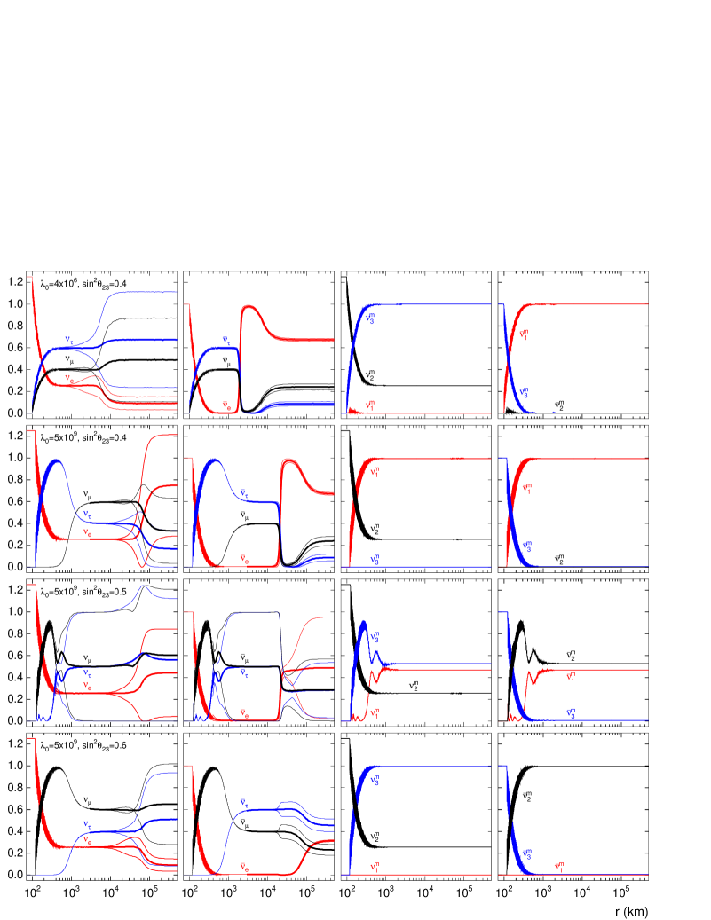
Figure 5.2: Radial evolution of the neutrino fluxes, normalized to the initial $\bar{\nu}_{e}$ flux, for a fixed neutrino energy ($E_{\nu}=20$ MeV) and an inverted $\Delta m^{2}_{\rm atm}$. From left to right: neutrino weak eigenstates, antineutrino weak eigenstates, neutrino propagation eigenstates and antineutrino propagation eigenstates. In the first two columns, after bipolar conversions we show the average as thick lines and the envelopes of the fast-oscillating curves as thin lines. The top row shows the case of a vanishing $\mu\tau$ matter effect, while the three bottom rows use a large $\mu\tau$ effect with different values for the 23 mixing angle as indicated [18].

As a first case we consider the traditional assumption of a vanishing $\mu\tau$ matter effect, which we account for using a value of $\lambda_{0}=4\times 10^{6}$. We assume an inverted $\Delta m^{2}_{\rm atm}$ and use a non-maximal value $\sin^{2}\theta_{23}=0.4$. Our numerical calculations for this case are shown in the top row of Fig. 5.2. The first two panels correspond to the radial evolution of the fluxes of the weak interaction eigenstates of neutrinos and antineutrinos, respectively, whereas in the last two panels we show the evolution of the propagation eigenstates. These are the eigenstates of $\Omega_{\bf p}+{\sf V}$, i.e., of that part of the Hamiltonian Eq. (6.31) that does not include the neutrino-neutrino interactions. In the collective neutrino region, we observe the usual pair conversion of the $\nu_{e}$ and $\bar{\nu}_{e}$ fluxes into the $\mu$ and $\tau$ flavors. Had we chosen a maximal $23$ mixing angle, the appearance curves for these flavors would be identical.

For larger distances the evolution consists of ordinary MSW transformations that are best pictured in the basis of instantaneous propagation eigenstates in matter (last two panels). Beyond the collective transformation region, all neutrinos and antineutrinos stay fixed in their propagation eigenstates. In the weak-interaction basis, on the other hand, this implies fast oscillations because we have a fixed energy, preventing kinematical decoherence between different energy modes. In the panels for neutrino and antineutrino interaction states, for radii beyond the dense-neutrino region we show as thick lines the average evolution as well as the envelopes of the fast-oscillating flavor fluxes.

Another way of describing this evolution is by the level crossing schemes of Fig. 5.3. The upper left panel represents the case of vanishing $V_{\mu\tau}$. The right panels represent the case with large $V_{\mu\tau}$ and a 23-mixing angle in the first octant (upper right panel) or second octant (bottom panel). These level crossing schemes are the same ones shown in Fig. 2.6 of Chapter 2, but adding the effect of collective transformations (vertical arrows). The upper (blue) line corresponds to propagation eigenstate 2, the middle (green) line to 1, and the bottom (red) line to 3, a scheme representing the inverted hierarchy case.

While in vacuum the propagation eigenstates coincide with the mass eigenstates, at large densities they correspond to weak interaction eigenstates. For vanishing $V_{\mu\tau}$ and at the low energies relevant to our problem, the $\mu$ and $\tau$ flavor are not distinguishable so that any convenient linear combination can be chosen as interaction eigenstates. It is convenient to introduce the states $\nu_{\mu}^{\prime}$ and $\nu_{\tau}^{\prime}$ that correspond to a vanishing 23-mixing angle, i.e., they diagonalize the 23-subsystem. If the small 13-mixing angle were to vanish, the 3-mass eigenstate would coincide with $\nu_{\tau}^{\prime}$. In the upper left panel of Fig. 5.3 and using the $(\nu_{e},\nu_{\mu}^{\prime},\nu_{\tau}^{\prime})$ basis, the 2-state connects adiabatically to $\nu_{e}$ and $\bar{\nu}_{\mu}^{\prime}$, whereas the 3-state connects adiabatically to $\bar{\nu}_{e}$ and $\nu_{\tau}^{\prime}$.

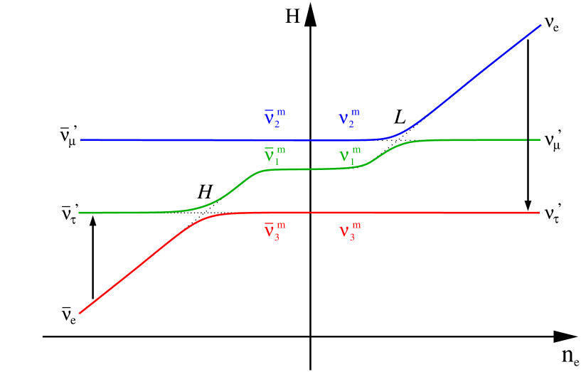
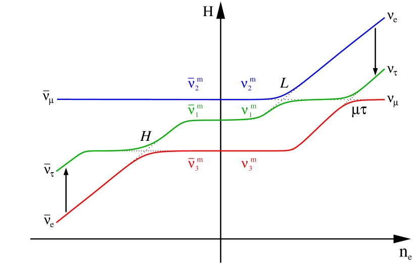
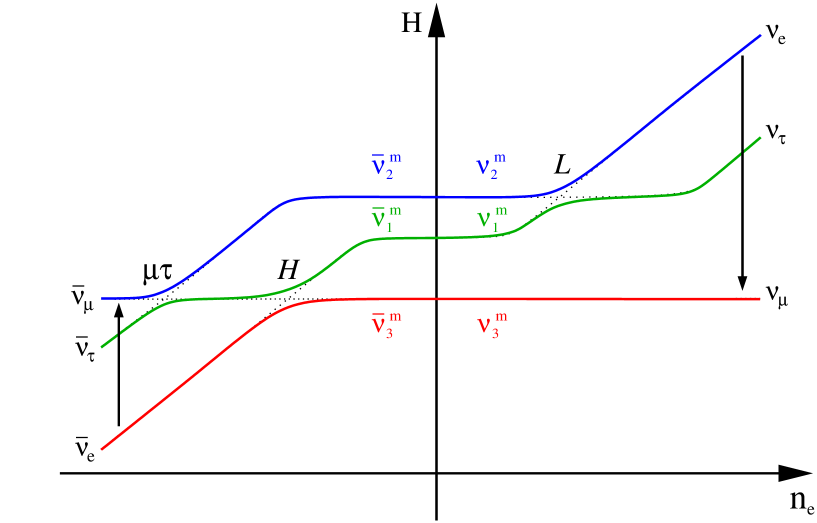
Figure 5.3: Level crossing scheme of neutrino conversion for the inverted hierarchy in a medium with a vanishing $V_{\mu\tau}$ (upper-left panel) and a large $V_{\mu\tau}$ with 23-mixing in the first octant (upper-right panel) or the second octant (bottom panel). The arrows indicate the transitions caused by collective flavor transformations [18].

At the neutrino sphere, the fluxes are prepared in $\nu_{e}$ and $\bar{\nu}_{e}$ eigenstates, which in the case of inverted mass hierarchy coincide with the propagation (or matter) eigenstates $\nu^{m}_{2}$ and $\bar{\nu}^{m}_{3}$, respectively. In the absence of neutrino-neutrino interactions, since the $L$-resonance is always adiabatic, the $\nu_{e}$’s leave the star as $\nu_{2}$. In the case of $\bar{\nu}_{e}$ the evolution depends on $\sin^{2}\theta_{13}$, see Fig. 2.7. For values larger than $10^{-3}$ they propagate also adiabatically (MSW transformation) and escape as $\bar{\nu}_{3}$, whereas for values smaller than $10^{-5}$ the transition at the $H$-resonance is strongly non-adiabatic: there is a jump of matter eigenstates from $\bar{\nu}^{m}_{3}$ to $\bar{\nu}^{m}_{1}$ and the $\bar{\nu}_{e}$’s leave the star as $\bar{\nu}_{1}$. As a consequence, the survival probability is $P(\nu_{e}\rightarrow\nu_{e})\approx\sin^{2}\theta_{12}$ and $P(\bar{\nu}_{e}\rightarrow\bar{\nu}_{e})\approx\sin^{2}\theta_{13}$ or $\cos^{2}\theta_{12}$ for large and small $\theta_{13}$, respectively.

In the presence of neutrino-neutrino interactions, important collective effects take place in the inner SN layers, where the neutrino density is high. We observe in the first two panels of Fig. 5.2 that collective pair transformations convert the $\nu_{e}$ and $\bar{\nu}_{e}$ fluxes to $\nu_{\tau}^{\prime}$ and $\bar{\nu}_{\tau}^{\prime}$ as indicated by the arrows in the upper left panel of Fig. 5.3. The consequences for the subsequent evolution are dramatic. In the case of $\nu_{e}$ a fraction equal to $\epsilon F_{\bar{\nu}_{e}}$ stays in $\nu_{2}^{m}$ and evolves as in the absence of neutrino-neutrino interactions, while the rest of $\nu_{e}$ are transformed to $\nu_{3}^{m}$. As a consequence, the final $\nu_{e}$ flux, normalized to the initial $\bar{\nu}_{e}$ one, is expected to be approximately $\epsilon\sin^{2}\theta_{12}\simeq 0.08$, see thick line in the upper left panel in Fig. 5.2. In the case of antineutrinos the effect of the collective pair conversion is to interchange the eigenstates in which $\bar{\nu}_{e}$ and $\bar{\nu}_{\tau}^{\prime}$ arrive at the $H$-resonance. Now $\bar{\nu}_{e}$ enters the resonance as $\bar{\nu}_{1}^{m}$ instead of $\bar{\nu}_{3}^{\rm m}$. Therefore, for $\sin^{2}\theta_{13}\gtrsim 10^{-3}$ the resonance is adiabatic and the $\bar{\nu}_{e}$’s leave the star as $\bar{\nu}_{1}$, leading to a final normalized flux of approximately $\cos^{2}\theta_{12}\simeq 0.68$, see the thick line in the second panel in Fig. 5.2. Instead, if $\sin^{2}\theta_{13}\lesssim 10^{-5}$ again there is a jump of matter eigenstates from $\bar{\nu}^{m}_{1}$ to $\bar{\nu}^{m}_{3}$ at the $H$-resonance. In this case $\bar{\nu}_{e}$ leaves the star as $\bar{\nu}_{3}$, leading to a normalized $\bar{\nu}_{e}$ flux equal to $\sin^{2}\theta_{13}$.

The impact of collective effects is easier to understand if we do as in the two-flavor system, where we have discussed that the impact of ordinary matter can be transformed away by going into a rotating reference frame for the polarization vectors. Collective conversions proceed in the same way as they would in vacuum, except that the effective mixing angle is reduced. Therefore, assuming an inverted hierarchy (IH) for the atmospheric mass splitting and a normal hierarchy (NH) for the solar splitting, we should consider the level scheme as in the upper left panel of Fig. 5.4. The mass eigenstates now approximately coincide with the interaction eigenstates because the 23-mixing angle was removed by going to the primed states, and the mixing angles involving $\nu_{e}$ are effectively made small by the presence of matter. Of course, this level scheme does not adiabatically connect to the true vacuum situation.

The initial state consists of $\nu_{e}$ and $\bar{\nu}_{e}$ and thus essentially of $\nu_{1}$ and $\bar{\nu}_{1}$. Collective conversions driven by $\Delta m^{2}_{\rm atm}$ then transform $\nu_{1}\bar{\nu}_{1}$ pairs to $\nu_{3}\bar{\nu}_{3}$ pairs in the familiar two-flavor way. If both hierarchies are normal, we begin in the lowest-lying state and nothing happens.

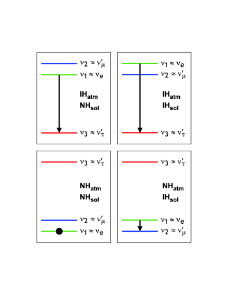
Figure 5.4: Vacuum level diagram for all hypothetical combinations of atmospheric and solar mass hierarchies (normal or inverted). The 12 and 13 mixing angles are assumed to be very small, mimicking the effect of ordinary matter. The effect of collective conversions is indicated by an arrow [18].

In the hypothetical case where both hierarchies are inverted (upper right panel in Fig. 5.4), we begin in the highest state and $\Delta m^{2}_{\rm atm}$ drives us directly to the lowest state. Finally, if the atmospheric hierarchy is normal and the solar one is inverted (lower right panel in Fig. 5.4), collective transformations driven by $\Delta m^{2}_{\rm sol}$ take us to the lowest state.

We have numerically solved the evolution of the three-flavor system with a realistic SN matter profile and found that the results confirm this simple picture. In a two-flavor treatment, the much smaller $\Delta m^{2}_{\rm sol}$ leads to collective transformations at a much larger radius than $\Delta m^{2}_{\rm atm}$. In a three-flavor treatment, $\Delta m^{2}_{\rm atm}$ therefore acts first and takes us directly to the lowest-lying state if the atmospheric hierarchy is inverted. Otherwise only the hypothetical case of the lower-right panel in Fig. 5.4 is an example where $\Delta m^{2}_{\rm sol}$ plays any role. We have numerically verified that normal $\Delta m_{\rm atm}^{2}$ combined with inverted $\Delta m_{\rm sol}^{2}$ is the only case where $\Delta m_{\rm sol}^{2}$ drives collective transformations. Since $\Delta m_{\rm sol}^{2}$ is measured to be normal, the previous two-flavor treatments based on $\Delta m_{\rm atm}^{2}$ and $\theta_{13}$ fortuitously capture the full effect.

We conclude that in the limit of a vanishing $\mu\tau$ effect the collective flavor transformations and the subsequent MSW evolution factorize and that the collective effects are correctly treated in a two-flavor picture. Of course, this situation may change if the matter profile is so low that the ordinary MSW effects occur in the same region as the collective phenomena [168].

5.4 Large mu-tau matter effect

Next we calculate the flavor evolution for the same model, now including a significant $V_{\mu\tau}$, i.e. we assume a large $\lambda_{0}$. In this case the flavor content of the neutrino and antineutrino fluxes emerging from the SN surface depend on the strength of $V_{\mu\tau}$ as well as the choice of $\theta_{23}$, as can be seen in the corresponding panels of Fig. 5.2. In this figure, one can also notice that the inclusion of $V_{\mu\tau}$ delays the onset of the bipolar conversions. We will discuss the latter effect in the next section, while here we will concentrate on the former one. This dependence is best illustrated with the help of the contour plot Fig. 5.5 where we show the $\nu_{e}$ and $\bar{\nu}_{e}$ fluxes emerging from the SN, averaged over fast vacuum oscillations.

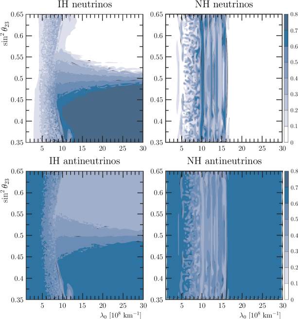
Figure 5.5: Contours in the space of $\sin^{2}\theta_{23}$ and $\lambda_{0}$ for the $\nu_{e}$ (top) and $\bar{\nu}_{e}$ (bottom) fluxes emerging from the SN surface for both normal (right) and inverted (left) mass hierarchy. All fluxes are normalized to the initial $\bar{\nu}_{e}$ flux. We show values averaged over fast vacuum oscillations [18].

If $V_{\mu\tau}$ is so large that the mu-tau effect is strong in the region of collective neutrino oscillations, there are two stable limiting cases, depending on the 23 mixing angle. If the mixing angle is sufficiently non-maximal and in the first octant, the collective oscillations transform the initially prepared $\nu_{e}$ and $\bar{\nu}_{e}$ fluxes to the propagation eigenstates as indicated by the arrows in the upper right panel of Fig. 5.3, i.e., we observe pair transformations to $\nu_{\tau}\bar{\nu}_{\tau}$.

This behavior is understood if we assume that in the $\mu\tau$ system we can once more go to a rotating frame and now simply imagine that the 23 mixing angle is effectively small by the impact of the $\mu\tau$ matter effect. In this case $\nu_{3}\approx\nu_{\tau}$. Since collective quasi-vacuum oscillations take us to the lowest-lying state, the $\nu_{3}$ state in the inverted hierarchy, we are effectively taken to $\nu_{\tau}\bar{\nu}_{\tau}$ pairs. Instead, if the 23 mixing angle is in the second octant, $\nu_{\mu}$ and $\nu_{\tau}$ switch roles, explaining that now $\nu_{3}\approx\nu_{\mu}$ and $\bar{\nu}_{3}\approx\bar{\nu}_{\mu}$.

For intermediate values of $V_{\mu\tau}$ and for 23 mixing angles near maximal, the final fluxes depend sensitively on parameters. For intermediate values of $V_{\mu\tau}$, there are also nontrivial effects for the normal hierarchy. The collective effects do not place the ensemble into propagation eigenstates, preventing a simple interpretation. The sensitive dependence for intermediate $V_{\mu\tau}$ is also illustrated in the top panels of Fig. 5.6 where we show the emerging average $\nu_{e}$ and $\bar{\nu}_{e}$ fluxes as functions of $\lambda_{0}$ for two values of $\theta_{23}$, one in the first and the other in the second octant. In the bottom panels of Fig. 5.6 we show the same $\nu_{e}$ and $\bar{\nu}_{e}$ fluxes as functions of $\sin^{2}\theta_{23}$ for $\lambda_{0}=1.85\times 10^{9}$ km^-1. One can notice how the fall of $\bar{\rho}_{ee}$ is not exactly centered at $\sin^{2}\theta_{23}=0.5$ but slightly shifted to smaller values. This is due to second-order corrections to the $\mu\tau$ resonance condition.

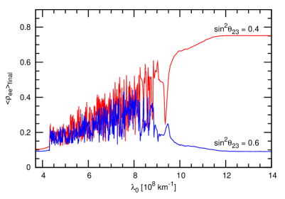
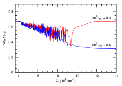
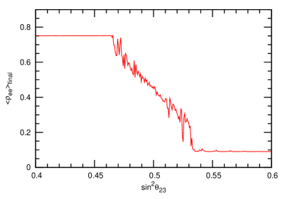
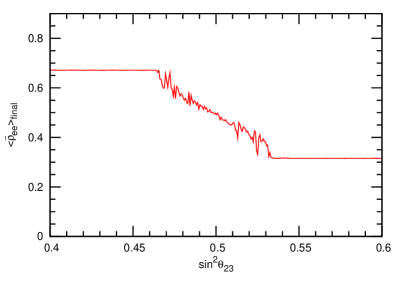
Figure 5.6: Fluxes of $\nu_{e}$ (left column) and $\bar{\nu}_{e}$ (right column), normalized to the initial $\bar{\nu}_{e}$ flux, emerging from the SN. The first row is done as a function of $\lambda_{0}$ for a 23 mixing angle in the first (red line) or second (blue line) octant, while the second row is represented as a function of $\sin^{2}\theta_{23}$ for $\lambda_{0}=1.85\times 10^{9}$ km^-1. These curves represent cuts through the inverted hierarchy contour plots of Fig. 5.5 at the indicated values of $\lambda_{0}$ and $\sin^{2}\theta_{23}$ [18].

This dependence on the $\theta_{23}$ octant leads to a clear imprint on the final survival probability. Let us first consider the first octant. In the case of $\nu_{e}$ a fraction equal to $\epsilon F_{\bar{\nu}_{e}}$ stays in $\nu_{2}^{m}$. However the presence of the $\mu\tau$-resonance in the neutrino channel makes the rest of the $\nu_{e}$ to be transformed to $\nu_{1}^{m}$. Their subsequent evolution would depend on the adiabaticity of the $\mu\tau$-resonance, but it has been shown to be always adiabatic [75]. As a consequence, the final $\nu_{e}$ flux is expected to be approximately $\cos^{2}\theta_{12}+\epsilon\sin^{2}\theta_{12}\simeq 0.76$, see thick line in the left panel of the second row in Fig. 5.2. In the case of antineutrinos the situation is completely analogous to the case of vanishing $V_{\mu\tau}$ so that $P(\bar{\nu}_{e}\rightarrow\bar{\nu}_{e})\approx\cos^{2}\theta_{12}$ or $\sin^{2}\theta_{13}$, depending on the value of $\theta_{13}$.

If $\theta_{23}$ belongs to the second octant, then the $\mu\tau$-resonance lies in the antineutrino channel. The crucial point is that now all $\bar{\nu}_{e}$ are transformed to $\bar{\nu}_{\mu}=\bar{\nu}_{2}^{m}$ before reaching the $\mu\tau$-resonance, see the lower panel in Fig. 5.3. Taking into account that $\bar{\nu}_{2}^{m}$ does not encounter the $H$-resonance, the survival probability will be always $P(\bar{\nu}_{e}\rightarrow\bar{\nu}_{e})\approx\sin^{2}\theta_{12}$, independently of the value of $\theta_{13}$. On the other hand neutrinos do not feel the $\mu\tau$-resonance and therefore their propagation is the same as in the vanishing $V_{\mu\tau}$ case.

We present in Table 5.1 a summary of the cases discussed so far. One can see the importance of the presence of collective neutrino effects, as well as the dependence on the strength of the mu-tau matter effect.

Table 5.1: Summary of the approximate values of the $\bar{\nu}_{e}$ survival probability for an inverted hierarchy, including or not collective effects. Here a small (large) mixing angle $\theta_{13}$ stands for $\sin^{2}\theta_{13}\lesssim 10^{-5}$ ($\sin^{2}\theta_{13}\gtrsim 10^{-3}$), while a small (large) $V_{\mu\tau}$ represents $r^{\mu\tau}_{\rm res}$ being smaller (larger) than $r_{\rm syn}$.

Collective	$V_{\mu\tau}$	$\theta_{23}$	$\theta_{13}$	$\bar{\nu}_{e}$	$P(\bar{\nu}_{e}\rightarrow\bar{\nu}_{e})$
effects				leaves as
no	any	any	small	$\bar{\nu}_{1}$	$\cos^{2}\theta_{12}$
no	any	any	large	$\bar{\nu}_{3}$	$\sin^{2}\theta_{13}$
yes	small	any	small	$\bar{\nu}_{3}$	$\sin^{2}\theta_{13}$
yes	small	any	large	$\bar{\nu}_{1}$	$\cos^{2}\theta_{12}$
yes	large	$<\pi/4$	small	$\bar{\nu}_{3}$	$\sin^{2}\theta_{13}$
yes	large	$<\pi/4$	large	$\bar{\nu}_{1}$	$\cos^{2}\theta_{12}$
yes	large	$>\pi/4$	any	$\bar{\nu}_{2}$	$\sin^{2}\theta_{12}$

5.5 Delay on the onset of bipolar conversions

Another interesting feature concerns the position of $r_{\rm syn}$ in the presence of a large $\mu\tau$ matter effect. As can be seen comparing the first two rows of Fig. 5.2, the radius where collective neutrino transformations begin is slightly larger ($r_{\rm syn}\simeq 115$ km) when we include a significant $V_{\mu\tau}$.

5.5.1 Rotation-averaged mass-squared matrix

As it was discussed in Sec. 4.4, when we include a background medium the oscillation frequency of the system is effectively modified, $\omega\to\omega\cos 2\theta$. In the usual two-flavor treatment of collective SN neutrino oscillations, driven by the small mixing angle $\theta_{13}$, this has little practical relevance because $\cos 2\theta\approx 1$ is a good approximation. In the realistic situation of three flavors, however, two of the mixing angles are large so that the projection effect of the squared masses caused by a large matter effect can become non-negligible. One particularly interesting case is the one we have been discussing in this chapter, when matter is so dense that the second-order difference between the $\nu_{\mu}$ and $\nu_{\tau}$ refractive effect is large. Here the matter effect encoded in the matrix ${\sf V}$ of the Hamiltonian Eq. (6.31) is large compared to the effect of the vacuum oscillation matrix ${\sf\Omega}={\sf M}^{2}/2E$. Going to the rotating three-flavor frame implies that all off-diagonal elements of ${\sf M}^{2}$ average to zero and we should think of all three weak-interaction eigenstates $\nu_{e}$, $\nu_{\mu}$ and $\nu_{\tau}$ as unmixed mass-eigenstate neutrinos with masses implied by the rotation-averaged ${\sf M}^{2}$.

To determine these effective mass-squares of the weak-interaction states we use the parametrization of the leptonic mixing matrix in terms of the usual mixing angles $\theta_{12}$, $\theta_{13}$, $\theta_{23}$, and the Dirac phase $\delta$. We here consider the inverted mass hierarchy that is most relevant for our study. For the vacuum mass-squares we use $m_{3}^{2}=0$, $m_{1}^{2}=\Delta m_{\rm atm}^{2}$ and $m_{2}^{2}=(1+a)\,\Delta m_{\rm atm}^{2}$, where

$$a=\frac{\Delta m^{2}_{\odot}}{\Delta m_{\rm atm}^{2}}=\frac{1}{30}$$ (5.8)

is the neutrino mass hierarchy parameter. We then find for the diagonal elements of ${\sf M}^{2}$ in the weak-interaction basis

$$\frac{m^{2}_{\nu_{e}}}{\Delta m^{2}_{\rm atm}} = \left(1+a\,s_{12}^{2}\right)\,c_{13}^{2}\,,$$

$$\frac{m^{2}_{\nu_{\mu}}}{\Delta m^{2}_{\rm atm}} = \left(1+a\,c_{12}^{2}\right)\,c_{23}^{2}-2a\,c_{12}\,c_{23}\,s_{12}\,s_{23}\,c_{\delta}\,s_{13}+\left(1+a\,s_{12}^{2}\right)\,s_{23}^{2}\,s_{13}^{2}\,,$$ (5.9)

$$\frac{m^{2}_{\nu_{\tau}}}{\Delta m^{2}_{\rm atm}} = \left(1+a\,c_{12}^{2}\right)\,s_{23}^{2}+2a\,c_{12}\,c_{23}\,s_{12}\,s_{23}\,c_{\delta}\,s_{13}+\left(1+a\,s_{12}^{2}\right)\,c_{23}^{2}\,s_{13}^{2}\,.$$

In the absence of any mixing, the r.h.s. would be 1, $1+a$, and 0 from top to bottom.

The 13–mixing angle is known to be small so that we have two small parameters, $s_{13}\ll 1$ and $a\ll 1$. In the second and third line both the second terms are of second order in small quantities and can be neglected. If in addition we use for the solar mixing angle $\theta_{12}=\pi/6$, the mass-squares are

$$\frac{m^{2}_{\nu_{e}}}{\Delta m^{2}_{\rm atm}} = 1+\frac{a}{4}\,,$$

$$\frac{m^{2}_{\nu_{\mu}}}{\Delta m^{2}_{\rm atm}} = \left(1+\frac{3a}{4}\right)\,\cos^{2}\theta_{23}\,,$$ (5.10)

$$\frac{m^{2}_{\nu_{\tau}}}{\Delta m^{2}_{\rm atm}} = \left(1+\frac{3a}{4}\right)\,\sin^{2}\theta_{23}\,.$$

The mass-squared spectrum, projected on the weak-interaction basis, depends most crucially on the mixing angle $\theta_{23}$ that is known to be nearly maximal. In principle, though, this mixing angle can vary in the range $0\leq\theta_{23}\leq\pi/2$. We show the projected mass spectrum as a function of $\theta_{23}$ in Fig. 5.7.

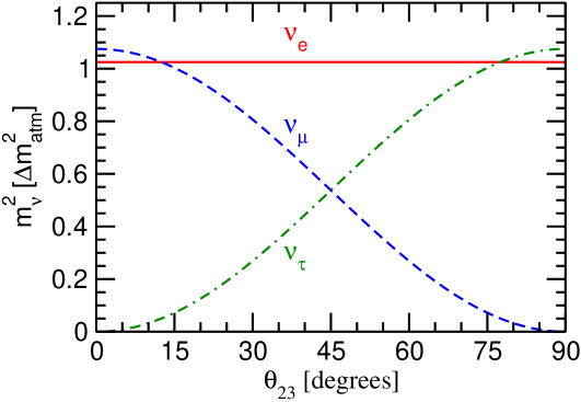
Figure 5.7: The diagonal elements of ${\sf M}^{2}$ in the weak-interaction basis as a function of $\theta_{23}$, assuming $\theta_{13}=0$ and $\theta_{12}=\pi/6$. To construct a legible plot, the mass-hierarchy parameter was chosen as $a=1/10$, although in reality it is $a\approx 1/30$.

5.5.2 Role of mu-tau matter effect

As a first case we return to the absence of a $\mu\tau$ matter effect. In this case mu and tau neutrinos are not distinguishable in the SN context. Therefore, we can re-define these flavors in the usual way as $\nu_{\mu}^{\prime}$ and $\nu_{\tau}^{\prime}$. This amounts to using the mass basis in the 23-system or rather, effectively to a situation of $\theta_{23}=0$. Therefore, the relevant mass spectrum driving collective oscillations is the one in Fig. 5.7 at $\theta_{23}=0$ and corresponds to the usual inverted-hierarchy spectrum, with the only modification that the splitting between the upper two neutrinos is not given by $\Delta m_{\rm sol}^{2}$, but only by half this amount because of the large 12–mixing angle. Corrections of order $a$ aside, collective oscillations are driven by $\Delta m^{2}_{\rm atm}$. This case corresponds essentially to the two-flavor example studied in Chapter 4. In Fig. 5.8 we show an analogous case in terms of the $\bar{\nu}_{e}$ survival probability, assuming $\omega=0.1~{}{\rm km}^{-1}$ and $\mu_{0}=10^{5}~{}{\rm km}^{-1}$, $\sin 2\theta=0.01$, $\epsilon=0.4$ and $\lambda=100~{}{\rm km}^{-1}$.

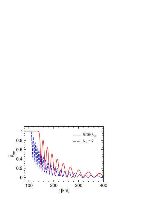
Figure 5.8: Radial variation of the numerical $\bar{\nu}_{e}$ survival probability and the adiabatic limit. Dashed lines: No $\mu\tau$ matter effect. Solid lines: Large $\mu\tau$ matter effect.

Next we consider the case of a large $\mu\tau$ matter effect where now we need to use the physical weak-interaction basis and not the primed states. In terms of Fig. 5.7 we now need to use $\theta_{23}=\pi/4$ or a value nearby within experimental errors. Therefore, we are now close to the cross-over between the $\nu_{\mu}$ and $\nu_{\tau}$ curves in Fig. 5.7. Therefore, the effective mass spectrum relevant for collective effects is now very different from the vacuum mass spectrum. In the absence of the $\mu\tau$ matter effect, the transitions were driven by

$$\omega=\frac{\Delta m^{2}_{\rm atm}}{2E}\,\left(1+\frac{a}{4}\right)\,.$$ (5.11)

Now, using $\theta_{23}=\pi/4$, they should be driven by

$$\omega^{\prime}=\frac{\Delta m^{2}_{\rm atm}}{2E}\,\frac{1}{2}\left(1-\frac{a}{4}\right)\,.$$ (5.12)

Therefore, the new oscillation frequency is predicted to be

$$\frac{\omega^{\prime}}{\omega}=\frac{4-a}{8(1-a)}=\frac{1}{2}+\frac{5}{8}\,a+{\cal O}(a^{2})\,.$$ (5.13)

According to Eq. (4.15) a change in the oscillation frequency automatically means a change in $r_{\rm syn}$. This is exactly what we obtain in Fig. 5.8, where we show the numerical solution for the case with a strong $\mu\tau$ matter effect together with the case of vanishing $\lambda_{\mu\tau}$.

Another test consists of returning to the case without a $\mu\tau$ matter effect and to modify $\omega\to\omega^{\prime}$ by hand. We find almost the same numerical curve as before, i.e., the impact of the $\mu\tau$ matter effect indeed essentially amounts to a modified mass-squared spectrum as predicted.

If we use $\theta_{23}<\pi/4$, the lowest effective mass eigenstate corresponds to $\nu_{\tau}$, for $\theta_{23}>\pi/4$ it corresponds to $\nu_{\mu}$. Collective oscillations always seem to go directly to the lowest mass eigenstate. We can repeat the above exercise for different values for $\theta_{23}$ and the corresponding $\omega^{\prime}$ and find a behavior consistent with expectations.

5.6 Competition between mu-tau and dense matter effects

We seem to have here a competition between two different effects, both result of large matter densities. On the one hand, we have shown in this chapter that the mu-tau matter effect could have important consequences in neutrinos streaming off a SN core if $V_{\mu\tau}$ is large in the collective region. On the other hand, in Sec. 4.4 we have studied the multi-angle matter effects in the collective neutrino transformations, obtaining a suppression of the bipolar conversions if the matter density is sufficiently large. Therefore we want to know if these effects happen at different density scales and will both be present, or on the contrary the multi-angle effects will destroy the interesting mu-tau matter effect.

In order to have an important mu-tau matter effect, we require

$$V_{\mu\tau}(r_{\rm bip})\gtrsim\omega_{\rm H}$$ (5.14)

where $r_{\rm bip}$ denotes the end of the bipolar conversion region, and we recall that $\omega_{\rm H}=\Delta m^{2}_{\rm atm}/2E$. Applying here Eq. (5.7) we obtain a lower limit for $\lambda_{0}$ leading to mu-tau matter effect,

$$\lambda_{0}\gtrsim\frac{\omega_{\rm H}}{Y^{\rm eff}_{\tau}}\left(\frac{r_{\rm bip}}{R_{\nu}}\right)^{3}\,.$$ (5.15)

For the typical values of the parameters we are assuming in our simulations ($\omega_{\rm H}=0.3$ km^-1, $Y^{\rm eff}_{\tau}=2.7\times 10^{-5}$ km^-1, $R_{\nu}=10$ km, and $r_{\rm bip}=330$ km) we obtain this limit to be $\lambda_{0}\gtrsim 4\times 10^{8}$ km^-1.

On the other hand, we have obtained in Eq. (4.62) that the collective transformations will be suppressed until

$$\lambda^{*}(r_{\rm syn})\lesssim\mu^{*}(r_{\rm syn})\,.$$ (5.16)

Noting that $\lambda^{*}=(R_{\nu}^{2}/2r^{2})\lambda$ (where $\lambda\equiv V_{\rm CC}$) and $\mu^{*}\approx\mu_{0}(R_{\nu}^{4}/2r^{4})$, we obtain an upper limit on $\lambda_{0}$ in order for the bipolar conversions to occur,

$$\lambda_{0}\lesssim\frac{\mu_{0}}{Y_{e}}\frac{r_{\rm syn}}{R_{\nu}}\,.$$ (5.17)

Applying our standard values ($\mu_{0}=7\times 10^{-5}$ km^-1, $Y_{e}=0.5$, $R_{\nu}=10$ km, and $r_{\rm syn}=100$ km) we get $\lambda_{0}=1.4\times 10^{7}$ km^-1.

These simple arguments seem to show that both effects take place for the same density scales, leaving no room for a coexistence between them. The suppression of collective transformations due to multi-angle effects in the dense matter region will destroy any possible effect coming from the $\mu\tau$-resonance.

5.7 Conclusions

At the relatively low energies relevant for SN neutrinos, charged mu and tau leptons cannot be produced so that mu- and tau-flavored neutrinos are not distinguishable in the SN or in detectors. (In the inner core of a SN the temperatures may be high enough to produce a significant thermal muon density, but this would not affect the emission from the neutrino sphere.) The impact of the small second-order difference between the $\nu_{\mu}$ and $\nu_{\tau}$ refractive index does not produce observable effects as long as one only considers the traditional MSW flavor conversion [75].

The picture changes if one includes the unavoidable effect of collective neutrino transformations in the region above the neutrino sphere. If the matter density is large enough that $V_{\mu\tau}$ is comparable to or larger than $\Delta m_{\rm atm}^{2}/2E$, the survival probability of $\nu_{e}$ and $\bar{\nu}_{e}$ can be completely modified and depends sensitively on the mixing angle $\theta_{23}$.

When it is important, the mu-tau matter effect adds one more layer of complication to the already vexed problem of collective SN neutrino oscillations. It was previously recognized that “ordinary” collective oscillations are almost completely insensitive to the smallness of $\theta_{13}$ as long as it is not exactly zero. Here we have found the opposite for the large mixing angle $\theta_{23}$ that is often assumed to be maximal. Even small deviations from maximal 23-mixing can imprint themselves in the collective oscillation effect. Both results are counter-intuitive and opposite to ordinary flavor oscillations.

It seems though, that the density requirement for this $\mu\tau$ effect to be important implies that the multi-angle matter effect can not be avoided. In this sense, one complicated effect caused by a large matter density annihilates another one.

Chapter 6 Non-Standard Neutrino Interactions in Supernova

In this chapter we investigate the impact of non-standard neutrino interactions on SN physics. We show how complementary information on the NSI parameters could be inferred from the detection of core-collapse SN neutrinos.

The motivation for the study is twofold. First, if a future SN explosion takes place in our Galaxy the number of neutrino events expected in the current or planned neutrino detectors would be enormous, $\mathcal{O}(10^{4}$–$10^{5})$ [189]. Moreover, the extreme conditions under which neutrinos have to travel since they are created in the SN core, in strongly deleptonized regions at nuclear densities, until they reach the Earth, lead to strong matter effects. In particular the effect of small values of the NSI parameters can be dramatically enhanced, possibly leading to observable consequences.

As we will later see, the inclusion of NSI to the SN scenario can lead to strong effects in the same inner layers where collective transformations take place. Therefore, in order to better understand the physics of the problem, we will not consider the neutrino background in the first part of this chapter, and focus on the NSI side. In the second part, however, we will switch on the neutrino self-interactions and study the interplay between these two effects.

6.1 Previous literature

According to the currently accepted SN paradigm, neutrinos are expected to play a crucial role in SN dynamics. Moreover, many future large neutrino detectors are currently being discussed [190]. The huge number of events, $\mathcal{O}(10^{4}$–$10^{5})$, that would be “seen” in these detectors indicates that a future SN in our Galaxy would provide a very sensitive probe of neutrino NSI effects. The presence of NSI can lead to important consequences for SN neutrino physics both in the highly dense core as well as in the envelope where neutrinos basically freely stream.

The role of non-forward neutrino scattering processes on heavy nuclei and free nucleons giving rise to flavor change within the SN core has been recently analyzed in Ref. [191, 192]. The main effect found was a reduction in the core electron fraction $Y_{e}$ during core collapse. A lower $Y_{e}$ would lead to a lower homologous core mass, a lower shock energy, and a greater nuclear photon-disintegration burden for the shock wave. By allowing a maximum $\Delta Y_{e}=-0.02$ it has been claimed that $\varepsilon_{e\alpha}\lesssim 10^{-3}$, where $\alpha=\mu,~{}\tau$ [192].

On the other hand it has been noted since long ago that the existence of NSI plays an important role in the propagation of SN neutrinos through the envelope leading to the possibility of a new resonant conversion in the innermost layers. In contrast to the well known MSW effect it would take place even for massless neutrinos [142]. Two basic ingredients are necessary: universal and flavor changing NSI. In the original scheme neutrinos were mixed in the leptonic charged current and universality was violated thanks to the effect of mixing with heavy gauge singlet leptons [80, 81]. Such resonance would induce strong neutrino flavor conversion both for neutrinos and antineutrinos simultaneously, possibly affecting the neutrino signal of the SN1987A as well as the possibility of having $r$-process nucleosynthesis. This was first quantitatively considered within a two-flavor $\nu_{e}$-$\nu_{\tau}$ scheme, and bounds on the relevant NSI parameters were obtained using both arguments [193].

One of the main features of such “massless” resonant conversion mechanism is that it requires the violation of universality, its position being determined only by the matter chemical composition, namely the value of the electron fraction $Y_{e}$, and not by the density. In view of the experimental upper bounds on the NSI parameters such a new resonance can only take place in the inner layers of the SN, near the neutrino sphere, where $Y_{e}$ takes its minimum values (few per cent), see Fig. 2.4. In this region the values of $Y_{e}$ are small enough to allow for resonance conversions to take place in agreement with existing bounds on the strengths of non-universal NSI parameters.

The SN physics implications of another type of NSI present in supersymmetric R-parity violating models have also been studied in Ref. [194], again for a system of two neutrinos. For definiteness NSI on $d$-quarks were considered, in two cases: (i) massless neutrinos without mixing in the presence of flavor-changing (FC) and non-universal (NU) NSIs, and (ii) neutrinos with eV masses and FC NSI. Different arguments have been used in order to constrain the parameters describing the NSI, namely, the SN1987A signal, the possibility to get successful $r$-process nucleosynthesis, and the possible enhancement of the energy deposition behind the shock wave to reactivate it.

On the other hand, NSI could also affect the propagation of neutrinos in the outer layers. This was considered in Refs. [195, 196, 197] in a three-neutrino mixing scenario for the case $Y_{e}>0.4$, typical for the outer SN envelope. Together with the assumption that $\varepsilon^{dV}_{\alpha\beta}\lesssim 10^{-2}$ this prevents the appearance of internal resonances in contrast to previous references. Motivated by supersymmetric theories without R-parity, in Ref. [195] the authors considered the effects of small-strength NSI with $d$-quarks. Following the formalism developed in Refs. [198, 199] they studied the corrections that such NSI would have on the expressions for the survival probabilities in the standard resonances MSW-H and MSW-L. A similar analysis was performed in Ref. [196] assuming Z-induced NSI interactions originated by additional heavy neutrinos. A phenomenological generalization of these results was carried out in Ref. [197]. The authors found an analytical compact expression for the survival probabilities in which the main effects of the NSI can be embedded through shifts of the mixing angles $\theta_{12}$ and $\theta_{13}$. In contrast to similar expressions found previously these directly apply to all mixing angles, and in the case with Earth matter effects. The main phenomenological consequence was the identification of a degeneracy between $\theta_{13}$ and $\varepsilon_{e\alpha}$, similar to the analogous “confusion” between $\theta_{13}$ and the corresponding NSI parameter noted to exist in the context of long-baseline neutrino oscillations [109, 110].

6.2 Neglecting neutrino background

We here reconsidered the general three-neutrino mixing scenario with NSI in the absence of a neutrino background, as it has been assumed in all previous literature. This first approach will help us to better understand the genuine effects of the NSI, and will be very useful for the complete analysis when considering neutrino self-interactions. In contrast to previous work [195, 196, 197], we have not restricted ourselves to large values of $Y_{e}$, discussing also small values present in the inner layers. This way our generalized description includes both the possibility of neutrinos having the “massless” NSI-induced resonant conversions in the inner layers of the SN envelope [142, 193, 194], as well as the “outer” oscillation-induced conversions [195, 196, 197]. However we have confined ourselves to values of $\varepsilon_{e\alpha}$ small enough not to lead to drastic consequences during the core collapse.

6.2.1 Neutrino evolution

In this section we describe the main ingredients of our analysis. Our emphasis will be on the use of astrophysically realistic SN density and $Y_{e}$ profiles. Their details, in particular their time dependence, are crucial in determining the way NSI affect the propagation of neutrinos in the SN medium.
A) Evolution equation
As discussed in Chapter 3, in an unpolarized medium the neutrino propagation in matter will be affected by the vector coupling constant of the NSI, $\varepsilon_{\alpha\beta}^{fV}=\varepsilon_{\alpha\beta}^{fL}+\varepsilon_{\alpha\beta}^{fR}$. The way the neutral current NSI modifies the neutrino evolution will be parametrized phenomenologically through the effective low-energy four-fermion operator described in Eq. (3.1). We also assume $\varepsilon^{f}_{\alpha\beta}\in\Re$, neglecting possible $CP$ violation in the new interactions.

Under these assumptions the Hamiltonian describing the SN neutrino evolution in the presence of NSI can be cast in the following form

$${\rm i}\frac{{\rm d}}{{\rm d}r}\nu_{\alpha}=\left(H_{\rm kin}+H_{\rm int}\right)_{\alpha\beta}\nu_{\beta}~{},$$ (6.1)

where we recall that $H_{\rm kin}$ stands for the kinetic term $H_{\rm kin}=U(M^{2}/2E)U^{\dagger}$, with $M^{2}={\rm diag}(m_{1}^{2},m_{2}^{2},m_{3}^{2})$, and $U$ the three-neutrino lepton mixing matrix [80] in the PDG convention [43] and with no $CP$ phases. The second term of the Hamiltonian accounts for the interaction of neutrinos with matter and can be split into two pieces,

$$H_{\rm int}=H^{\rm std}_{\rm int}+H^{\rm nsi}_{\rm int}~{}.$$ (6.2)

Here, $H^{\rm std}_{\rm int}$ describes the standard interaction with matter and can be written as $H^{\rm std}_{\rm int}$ = diag $(V_{\rm CC},0,0)$ up to one loop corrections due to different masses of the muon and tau leptons, unimportant for this analysis. The standard matter potential for neutrinos is given by Eq. (2.38):

$$V_{\rm CC} = \sqrt{2}G_{F}N_{e}=V_{0}\rho Y_{e}~{},$$ (6.3)

where $V_{0}\approx 7.6\times 10^{-14}$ eV, the density is given in ${\rm g/cm}^{3}$, and $Y_{e}$ stands for the relative number of electrons with respect to baryons. For antineutrinos the potential is identical but with the sign changed.

The term in the Hamiltonian describing the non-standard neutrino interactions with a fermion $f$ can be expressed as,

$$(H_{\rm int}^{\rm nsi})_{\alpha\beta}=\sum_{f=e,u,d}(V_{\rm nsi}^{f})_{\alpha\beta}~{},$$ (6.4)

with $(V_{\rm nsi}^{f})_{\alpha\beta}\equiv\sqrt{2}G_{F}N_{f}\varepsilon^{f}_{\alpha\beta}$. For definiteness and motivated by actual models, for example, those with broken R-parity supersymmetry we take for $f$ the down-type quark. However, an analogous treatment would apply to the case of NSI on up-type quarks (see below). The existence of NSI with electrons brings no drastic qualitative differences with respect to the pure oscillation case. Therefore the NSI potential can be expressed as follows,

$$(V_{\rm nsi}^{d})_{\alpha\beta}=\varepsilon^{d}_{\alpha\beta}V_{0}\rho(2-Y_{e})~{}.$$ (6.5)

From now on we will not explicitely write the superindex $d$. In order to further simplify the problem we will redefine the diagonal NSI parameters so that $\varepsilon_{\mu\mu}=0$, as one can easily see that subtracting a matrix proportional to the identity leaves the physics involved in the neutrino oscillation unaffected.
B) Supernova matter profiles
Neutrino propagation depends on the SN matter and chemical profile through the effective potential. As it was discussed in Sec. 2.3.1, this profile exhibits an important time dependence during the explosion, see Fig. 2.4. We will use the parameterization given there for the density $\rho(t,r)$ and the electron fraction $Y_{e}(t,r)$ profiles. Progenitor density profiles can be roughly parameterized by the power-law function given in Eq. (2.74):

$$\rho(r)=\rho_{0}\left(\frac{r_{0}}{r}\right)^{n}~{},$$ (6.6)

where $\rho_{0}\sim 10^{4}$ g/cm³, $r_{0}\sim 10^{9}$ cm, and $n\sim 3$. While the electron fraction profile can be phenomenologically approximated by Eq. (2.75):

$$Y_{e}=a+b\arctan[(r-r_{0})/r_{s}]~{},$$ (6.7)

where $a\approx 0.23$–$0.26$ and $b\approx 0.16$–$0.20$. We recall that the parameters $r_{0}$ and $r_{s}$ describe where the rise takes place and how steep it is, respectively.

6.2.2 The two regimes

In order to study the neutrino propagation through the SN envelope we will split the problem into two different regions: the inner envelope, defined by the condition $V_{\rm CC}\gg\Delta m^{2}_{\rm atm}/(2E)$, and the outer one, where $\Delta m^{2}_{\rm atm}/(2E)\gtrsim V_{\rm CC}$. From the upper panel of Fig. 2.4 one can see how the boundary roughly varies between $r\approx 10^{8}$ cm and $10^{9}$ cm, depending on the time considered. This way one can fully characterize all resonances that can take place in the propagation of SN neutrinos, both the outer resonant conversions related to neutrino masses and indicated as the upper bands in Fig. 2.4, and the inner resonances that follow from the presence of NSI. Here we pay special attention to the use of realistic matter and chemical SN profiles and three-neutrino flavors thus generalising previous studies.
A) Neutrino evolution in the inner regions
Let us first write the Hamiltonian in the inner layers, where $H_{\rm int}\gg H_{\rm kin}$. In this case the Hamiltonian can be written as

$$H\approx H_{\rm int}=V_{0}\rho(2-Y_{e})\left(\begin{array}[]{ccc}\frac{Y_{e}}{2-Y_{e}}+\varepsilon_{ee}&\varepsilon_{e\mu}&\varepsilon_{e\tau}\\ \varepsilon_{e\mu}&0&\varepsilon_{\mu\tau}\\ \varepsilon_{e\tau}&\varepsilon_{\mu\tau}&\varepsilon_{\tau\tau}\end{array}\right)~{}.$$ (6.8)

When the value of the $\varepsilon_{\alpha\beta}$ is of the same order as the electron fraction $Y_{e}$ internal resonances can arise [142]. Taking into account the current constraints on the $\varepsilon$’s discussed in Chapter 3 one sees that small values of $Y_{e}$ are required [193, 194]. As a result, these can only take place in the most deleptonised inner layers, close to the neutrino sphere, where the kinetic terms of the Hamiltonian are negligible.

Given the large number of free parameters $\varepsilon_{\alpha\beta}$ involved we consider one particular case where $|\varepsilon_{e\mu}|$ and $|\varepsilon_{e\tau}|$ are small enough to neglect a possible initial mixing between $\nu_{e}$ and $\nu_{\mu}$ or $\nu_{\tau}$. Barring fine tuning, this basically amounts to $|\varepsilon_{e\mu}|,~{}|\varepsilon_{e\tau}|\ll 10^{-2}$. According to the discussion of Chapter 3, $\varepsilon_{e\mu}$ automatically satisfies the condition, whereas one expects that the window $|\varepsilon_{e\tau}|\gtrsim 10^{-2}$ will eventually be probed in future experiments.

Since the initial fluxes of $\nu_{\mu}$ and $\nu_{\tau}$ are expected to be basically identical, it is convenient to redefine the weak basis by performing a rotation in the $\mu$-$\tau$ sector:

$$\left(\begin{array}[]{c}\nu_{e}\\ \nu_{\mu}\\ \nu_{\tau}\end{array}\right)=U(\theta_{23}^{\prime})\left(\begin{array}[]{c}\nu_{e}\\ \nu_{\mu}^{\prime}\\ \nu_{\tau}^{\prime}\end{array}\right)=\left(\begin{array}[]{ccc}1&0&0\\ 0&c_{23^{\prime}}&s_{23^{\prime}}\\ 0&-s_{23^{\prime}}&c_{23^{\prime}}\end{array}\right)\left(\begin{array}[]{c}\nu_{e}\\ \nu_{\mu}^{\prime}\\ \nu_{\tau}^{\prime}\end{array}\right)~{},$$ (6.9)

where $c_{23^{\prime}}$ and $s_{23^{\prime}}$ stand for $\cos(\theta_{23}^{\prime})$ and $\sin(\theta_{23}^{\prime})$, respectively. The angle $\theta_{23}^{\prime}$ can be written as

$$\tan(2\theta_{23}^{\prime})\approx\frac{2H_{23}}{H_{33}}=\frac{2\varepsilon_{\mu\tau}}{\varepsilon_{\tau\tau}}~{}.$$ (6.10)

The Hamiltonian becomes in the new basis

$$H^{\prime}_{\alpha\beta}=U^{\dagger}(\theta_{23}^{\prime})H_{\alpha\beta}U(\theta_{23}^{\prime})=V_{0}\rho(2-Y_{e})\left(\begin{array}[]{ccc}\frac{Y_{e}}{2-Y_{e}}+\varepsilon_{ee}&\varepsilon_{e\mu}^{\prime}&\varepsilon_{e\tau}^{\prime}\\ \varepsilon_{e\mu}^{\prime}&\varepsilon_{\mu\mu}^{\prime}&0\\ \varepsilon_{e\tau}^{\prime}&0&\varepsilon_{\tau\tau}^{\prime}\end{array}\right)~{},$$ (6.11)

where

$$\varepsilon_{e\mu}^{\prime} = \varepsilon_{e\mu}c_{23^{\prime}}-\varepsilon_{e\tau}s_{23^{\prime}}$$ (6.12)

$$\varepsilon_{e\tau}^{\prime} = \varepsilon_{e\mu}s_{23^{\prime}}+\varepsilon_{e\tau}c_{23^{\prime}}$$ (6.13)

$$\varepsilon_{\mu\mu}^{\prime} = (\varepsilon_{\tau\tau}-\sqrt{\varepsilon^{2}_{\tau\tau}+4\varepsilon^{2}_{\mu\tau}})/2~{}$$ (6.14)

$$\varepsilon_{\tau\tau}^{\prime} = (\varepsilon_{\tau\tau}+\sqrt{\varepsilon^{2}_{\tau\tau}+4\varepsilon^{2}_{\mu\tau}})/2~{}.$$ (6.15)

With our initial assumptions on $\varepsilon_{e\alpha}$ one notices that the new basis $\nu_{\alpha}^{\prime}$ essentially diagonalizes the Hamiltonian, and therefore coincides roughly with the matter eigenstate basis. A novel resonance can arise if the condition $H_{ee}^{\prime}=H_{\tau\tau}^{\prime}$ is satisfied, we call this $I$-resonance, $I$ standing for “internal”. The alternative condition $H_{ee}^{\prime}=H_{\mu\mu}^{\prime}$ would give rise to another internal resonance which can be studied using the same method. The corresponding resonance condition can be written as

$$Y_{e}^{I}=\frac{2\varepsilon^{I}}{1+\varepsilon^{I}}~{},$$ (6.16)

where $\varepsilon^{I}$ is defined as $\varepsilon_{\tau\tau}^{\prime}-\varepsilon_{ee}$.

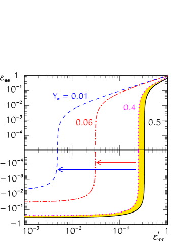
Figure 6.1: Contours of $Y_{e}^{I}$ as function of $\varepsilon_{ee}$ and $\varepsilon_{\tau\tau}^{\prime}$ according to Eq. (6.43) for different values of $Y_{e}$. The region in yellow represents the region of parameters that gives rise to $I$-resonance before the collapse. The arrows indicate how this region widens with time [21].

In Fig. 6.1 we represent the range of $\varepsilon_{ee}$ and $\varepsilon_{\tau\tau}^{\prime}$ leading to the $I$-resonance for an electron fraction profile between different $Y_{e}^{\rm min}$’s and $Y_{e}^{\rm max}=0.5$. It is important to notice that the value of $Y_{e}^{\rm min}$ depends on time, as discussed in Sec. 2.3.1. Right before the collapse the minimum value of the electron fraction is around $0.4$. Hence the window of NSI parameters that would lead to a resonance would be relatively narrow, as indicated by the shaded (yellow) band in Fig. 6.1. As time goes on $Y_{e}^{\rm min}$ decreases to values of the order of a few %, and as a result the region of parameters giving rise to the $I$-resonance significantly widens. For example, in the range $|\varepsilon_{ee}|\leq 10^{-3}$ possibly accessible to future experiments one sees that the $I$-resonance can take place for values of $\varepsilon_{\tau\tau}^{\prime}$ of the order of $\mathcal{O}(10^{-2})$. This indicates that the potential sensitivity on NSI parameters that can be achieved in SN studies is better than that of the current limits. One can see in Fig. 2.4 in order to fulfill the $I$-resonance condition for such small values of the NSI parameters the values of $Y_{e}$ must indeed lie, as already stated, in the inner layers.

Several comments are in order: First, in contrast to the standard $H$- and $L$-resonances, related to the kinetic term, the density itself does not explicitly enter into the resonance condition, provided that the density is high enough to neglect the kinetic terms. Analogously the energy plays no role in the resonance condition, which is determined only by the electron fraction $Y_{e}$. Moreover, in contrast to the standard resonances, the $I$-resonance occurs for both neutrinos and antineutrinos simultaneously [142]. Finally, as indicated in Fig. 6.2

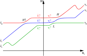
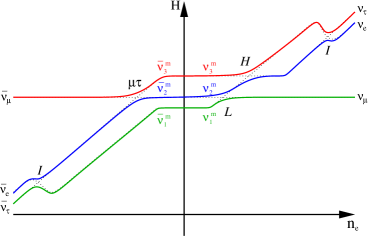
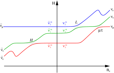
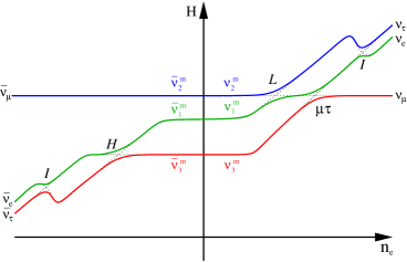
Figure 6.2: Level-crossing schemes, first panel is for the case of normal hierarchy (oscillations only), the second includes the NSI effect. The two lower panels correspond to the inverse hierarchy, oscillations only and oscillations + NSI, respectively.

the $\nu_{e}$’s ($\bar{\nu}_{e}$) are not created as the heaviest (lightest) state but as the intermediate state, therefore the flavor composition of the neutrinos arriving at the $H$-resonance is exactly the opposite of the case without NSI.

In order to calculate the hopping probability between matter eigenstates at the $I$-resonance we use the Landau-Zener approximation for two flavors, see Eq. (2.70),

$$P_{LZ}^{I}\approx e^{-\frac{\pi}{2}\gamma_{I}}~{},$$ (6.17)

where $\gamma_{I}$ stands for the adiabaticity parameter, defined in Eq. (2.57), generally written as

$$\gamma_{I}=\left|\frac{E_{2}^{\rm m}-E_{1}^{\rm m}}{2\dot{\theta}^{\rm m}}\right|_{r_{I}}~{},$$ (6.18)

with $\dot{\theta}^{\rm m}\equiv{\rm d}\theta^{\rm m}/{\rm d}r$. If one applies this formula to the $e-\tau^{\prime}$ box of Eq. (6.11) assuming that $\tan 2\theta^{\rm m}_{I}=2H_{e\tau}^{\prime}/(H_{\tau\tau}^{\prime}-H_{ee})$ and $E_{2}^{\rm m}-E_{1}^{\rm m}=\left[(H_{\tau\tau}^{\prime}-H_{ee})^{2}+4H_{e\tau}^{\prime}\right]^{1/2}$ one gets

$$\gamma_{I}=\left|\frac{4H_{e\tau}^{\prime 2}}{(\dot{H}_{\tau\tau}^{\prime}-\dot{H}_{ee})}\right|_{r_{I}}=\left|\frac{16V_{0}\rho\varepsilon_{e\tau}^{\prime 2}}{(1+\varepsilon^{I})^{3}\dot{Y}_{e}}\right|_{r_{I}}\approx 4\times 10^{9}r_{s,5}\rho_{11}\varepsilon_{e\tau}^{\prime 2}f(\varepsilon^{I})~{},$$ (6.19)

where the parametrization of the $Y_{e}$ profile has been defined as in Eq. (2.75) with $b=0.16$. The density $\rho_{11}$ represents the density in units of $10^{11}$ g/cm³, $r_{s,5}$ stands for $r_{s}$ in units of $10^{5}$ cm, and $f(\varepsilon^{I})$ is a function whose value is of the order $\mathcal{O}(1)$ in the range of parameters we are interested in. Taking all these factors into account it follows that the internal resonance will be adiabatic, provided that $\varepsilon_{e\tau}^{\prime}\gtrsim 10^{-5}$. This value is well below the current limits and in full numerical agreement with, e.g., Ref. [194].

In Fig. 6.3 we show the resonance condition as well as the adiabaticity in terms of $\varepsilon_{\tau\tau}$ and $\varepsilon_{e\tau}$ assuming the other $\varepsilon_{\alpha\beta}=0$. In order to illustrate the dependence on time we consider profiles inspired in the numerical profiles of Fig. 2.4 at $t=2$ s (left panel) and 15.7 s (right panel). For definiteness we take $Y_{e}^{\rm min}$ as the electron fraction at which the density has value of $5\times 10^{11}$g/cm³. For comparison with Fig. 6.1 we have assumed $Y_{e}^{\rm min}=10^{-2}$ in the case of 15.7 s. We observe how the border of adiabaticity depends on $\varepsilon_{\tau\tau}$ through the value of the density at $r_{I}$ which in turn depends on time.

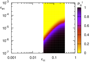
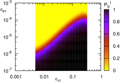
Figure 6.3: Contours of constant jump probability at the $I$-resonance in terms of $\varepsilon_{\tau\tau}$ and $\varepsilon_{e\tau}$ for two profiles corresponding to Fig. 2.4 at $2$ s with $a=0.235$ and $b=0.175$ (left panel) and $15.7$ s with $a=0.26$ and $b=0.195$ (right panel). For simplicity the other $\varepsilon$’s have been set to zero [21].

Before moving to the discussion of the outer resonances a comment is in order, namely, how does the formalism change for other non-standard interaction models. First note that the whole treatment presented above also applies to the case of NSI on up-type quarks, except that the position of the internal resonance shifts with respect to the down-quark case. Indeed, in this case the NSI potential

$$(V_{\rm nsi}^{u})_{\alpha\beta}=\varepsilon^{u}_{\alpha\beta}V_{0}\rho(1+Y_{e})~{},$$ (6.20)

would induce a similar internal resonance for the condition $Y_{e}=\varepsilon^{I}/(1-\varepsilon^{I})$.

In contrast, for the case of NSI with electrons, the NSI potential is proportional to the electron fraction, and therefore no internal resonance would appear.
B) Neutrino evolution in the outer regions
As it has been extensively discussed, in the outer layers of the SN envelope neutrinos can undergo important flavor transitions at those points where the matter induced potential equals the kinetic terms. In absence of NSI this condition can be expressed as $V_{\rm CC}\approx\Delta m^{2}/(2E)$. Therefore, two different resonance layers arise, the so-called $H$-resonance and the $L$-resonance, corresponding to the atmospheric and solar squared mass diferences, respectively.

The presence of NSI with values of $|\varepsilon_{\alpha\beta}|\lesssim 10^{-2}$ modifies the properties of the $H$- and $L$-transitions [195, 196, 197]. In particular one finds that the effects of the NSI can be described as in the standard case by embedding the $\varepsilon$’s into effective mixing angles [197]. An analogous “confusion” between $\sin\theta_{13}$ and the corresponding NSI parameter $\varepsilon_{e\tau}$ has been pointed out in the context of long-baseline neutrino oscillations in Refs. [109, 110].

In this section we perform a more general and complementary study for slightly higher values of the NSI parameters: $|\varepsilon_{\alpha\beta}|\gtrsim{\rm few}\times 10^{-2}$, still allowed by current limits, and for which the $I$-resonance could occur.

The phenomenological assumption of a hierarchy in the squared mass differences, $|\Delta m^{2}_{\rm atm}|\gg\Delta m^{2}_{\odot}$, allows, for not too large $\varepsilon$’s, a factorization of the 3$\nu$ dynamics into two 2$\nu$ subsystems roughly decoupled for the $H$- and $L$-transitions [200]. To isolate the dynamics of the $H$-transition, one usually rotates the neutrino flavor basis by $U^{\dagger}(\theta_{23})$, and extracts the submatrix with indices (1,3) [195, 197]. Whereas this method works perfectly for small values of $\varepsilon_{\alpha\beta}$ it can be dangerous for values above $10^{-2}$. In order to analyze how much our case deviates from the simplest approximation we have performed a rotation with the angle $\theta_{23}^{\prime\prime}\equiv\theta_{23}-\alpha$ instead of just $\theta_{23}$. By requiring that the new rotation diagonalizes the submatrix (2,3) at the $H$-resonance layer one obtains the following expression for the correction angle $\alpha$

$$\tan(2\alpha) = \left[\Delta_{\odot}s2_{12}s_{13}+V_{\tau\tau}^{nsi}s2_{23}-2V_{\mu\tau}^{nsi}c2_{23}\right]/$$

$$\left[(\Delta_{\rm atm}+\frac{1}{2}\Delta_{\odot})c^{2}_{13}+\frac{1}{4}\Delta_{\odot}c2_{12}(-3+c2_{13})+V_{\tau\tau}^{nsi}c2_{23}+2V_{\mu\tau}^{nsi}s2_{23}\right]~{},$$

where $\Delta_{\rm atm}\equiv\Delta m^{2}_{\rm atm}/(2E)$ and $\Delta_{\odot}\equiv\Delta m^{2}_{\odot}/(2E)$. In our notation $s_{ij}$ and $s2_{ij}$ represent $\sin\theta_{ij}$ and $\sin(2\theta_{ij})$, respectively. The parameters $c_{ij}$ and $c2_{ij}$ are analogously defined. In the absence of NSI $\alpha$ is just a small correction to $\theta_{23}$,

$$\tan(2\alpha)\approx\Delta_{\odot}s2_{12}s_{13}/\Delta_{\rm atm}c^{2}_{13}\lesssim\mathcal{O}(10^{-3})~{}.$$ (6.22)

In order to calculate $\alpha$ we need to know the $H$-resonance point. To calculate it one can proceed as in the case without NSI, namely, make the $\theta_{23}^{\prime\prime}$ rotation and analyze the submatrix $(1,3)$. The new Hamiltonian $H_{\alpha\beta}^{\prime\prime}$ has now the form

$$H_{ee}^{\prime\prime} = V_{0}\rho[Y_{e}+\varepsilon_{ee}(2-Y_{e})]+\Delta_{\rm atm}s^{2}_{13}+\Delta_{\odot}(c^{2}_{13}s^{2}_{12}+s^{2}_{13})~{},$$

$$H_{\tau\tau}^{\prime\prime} = V_{0}\rho(2-Y_{e})\varepsilon_{\tau\tau}^{\prime\prime}+\Delta_{\rm atm}c^{2}_{13}c^{2}_{\alpha}+\Delta_{\odot}\left[c^{2}_{13}c^{2}_{\alpha}+(s_{\alpha}c_{12}+c_{\alpha}s_{12}s_{13})^{2}\right]~{},~{}~{}~{}~{}$$ (6.23)

$$H_{e\tau}^{\prime\prime} = V_{0}\rho(2-Y_{e})\varepsilon_{e\tau}^{\prime\prime}+\frac{1}{2}\Delta_{\rm atm}s2_{13}c_{\alpha}+\frac{1}{2}\Delta_{\odot}(-c_{13}s_{\alpha}s2_{12}+c^{2}_{12}c_{\alpha}s2_{13})~{}.$$

We have defined $\varepsilon_{\tau\tau}^{\prime\prime}=\varepsilon_{\tau\tau}c^{2}_{23-\alpha}+\varepsilon_{\mu\tau}s2_{23-\alpha}$, and $\varepsilon_{e\tau}^{\prime\prime}=\varepsilon_{e\tau}c_{23-\alpha}+\varepsilon_{e\mu}s_{23-\alpha}$, where $s_{23-\alpha}\equiv\sin(\theta_{23}-\alpha),~{}c_{23-\alpha}\equiv\cos(\theta_{23}-\alpha)$, and $s2_{23-\alpha}\equiv\sin(2\theta_{23}-2\alpha),~{}c2_{23-\alpha}\equiv\cos(2\theta_{23}-2\alpha)$. The resonance condition for the $H$-transition, $H_{ee}^{\prime\prime}=H_{\tau\tau}^{\prime\prime}$ can be then written as

$$V_{0}\rho^{H}[Y_{e}^{H}+(\varepsilon_{ee}-\varepsilon_{\tau\tau}^{\prime\prime})(2-Y_{e}^{H})]=$$

$$\Delta_{\rm atm}(c^{2}_{13}c^{2}_{\alpha}-s^{2}_{13})+\Delta_{\odot}[c^{2}_{12}(c^{2}_{13}-c^{2}_{\alpha}s^{2}_{13})-s^{2}_{\alpha}s^{2}_{12}+\frac{1}{2}s2_{\alpha}s2_{12}s_{13}]~{}.$$ (6.24)

It can be easily checked how in the limit of $\varepsilon_{\alpha\beta}\to 0$ one recovers the standard resonance condition,

$$V_{0}\rho^{H}Y_{e}^{H}\approx\Delta_{\rm atm}c2_{13}~{}.$$ (6.25)

In the region where the $H$-resonance occurs $Y_{e}^{H}\approx 0.5$.

Taking into account Eqs. (6.2.2) and (6.24) one can already estimate how the value of $\alpha$ changes with the NSI parameters. In Fig. 6.4 we show the dependence of $\alpha$ on the $\varepsilon_{\tau\tau}$ after fixing the value of the other NSI parameters. One can see how for $\varepsilon_{\tau\tau}\gtrsim 10^{-2}$ the approximation of neglecting $\alpha$ significantly worsens. Assuming $\theta_{23}=\pi/4$ and a fixed value of $\varepsilon_{\mu\tau}$ one can easily see that $\varepsilon_{\tau\tau}$ basically affects the numerator in Eq. (6.2.2). Therefore one expects a rise of $\alpha$ as the value of $\varepsilon_{\tau\tau}$ increases, as seen in Fig. 6.4. The dependence of $\alpha$ on $\varepsilon_{\mu\tau}$ is correlated to the relative sign of the mass hierarchy and $\varepsilon_{\mu\tau}$. For instance, for normal mass hierarchy and positive values of $\varepsilon_{\mu\tau}$ the dependence is inverse, namely, higher values of $\varepsilon_{\mu\tau}$ lead to a suppression of $\alpha$. Apart from this general behavior, $\alpha$ also depends on the diagonal term $\varepsilon_{ee}$ as seen in Fig. 6.4. This effect occurs by shifting the resonance point through the resonance condition in Eq. (6.24).

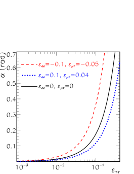
Figure 6.4: Angle $\alpha$ as function of $\varepsilon_{\tau\tau}$ for different values of $\varepsilon_{ee}$ and $\varepsilon_{\mu\tau}$, in the case of neutrinos of energy $10$ MeV, with normal mass hierarchy, and $s^{2}_{13}=10^{-5}$. The other NSI parameters take the following values: $\varepsilon_{e\mu}=0$ and $\varepsilon_{e\tau}=10^{-3}$ [21].

One can now calculate the jump probability between matter eigenstates in analogy to the standard case by means of the Landau-Zener approximation, see Eqs. (2.70) and (2.93),

$$P_{LZ}^{H}\approx e^{-\frac{\pi}{2}\gamma_{H}}~{},$$ (6.26)

where $\gamma_{H}$ represents the adiabaticity parameter at the $H$-resonance, which can be written as

$$\gamma_{H}=\left|\frac{4H_{e\tau}^{\prime\prime 2}}{(\dot{H}_{\tau\tau}^{\prime\prime}-\dot{H}_{ee}^{\prime\prime})}\right|_{r_{H}}~{},$$ (6.27)

where the expressions for $H_{\alpha\beta}^{\prime\prime}$ are given in Eqs (6.2.2).

Let us first consider the case $|\varepsilon_{\alpha\beta}|\lesssim 10^{-2}$. In this case $\alpha\approx 0$ and one can rewrite the adiabaticity parameter as

$$\gamma_{H}\approx\frac{\Delta_{\rm atm}\sin^{2}(2\theta_{13}^{eff})}{\cos(2\theta_{13}^{eff})|{\rm d}\ln V/{\rm d}r|_{r_{H}}}~{},$$ (6.28)

where

$$\theta_{13}^{eff}=\theta_{13}+\varepsilon_{e\tau}^{\prime\prime}(2-Y_{e})/Y_{e}$$ (6.29)

in agreement with Ref. [197].

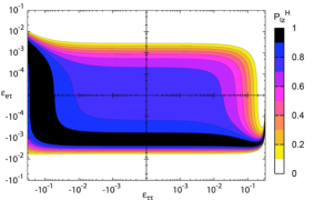
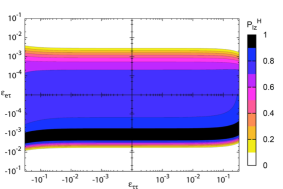
Figure 6.5: Landau-Zener jump probability isocontours at the $H$-resonance in terms of $\varepsilon_{e\tau}$ and $\varepsilon_{\tau\tau}$ for $10$ MeV antineutrinos in the case of inverted mass hierarchy. Left panel: $\alpha$ given by Eq. (6.2.2). Right panel: $\alpha$ set to zero. The remaining parameters take the following values: $\sin^{2}\theta_{13}=10^{-5},~{}\varepsilon_{ee}=\varepsilon_{e\mu}=\varepsilon_{\mu\tau}=0$. See text [21].

For slightly larger $\varepsilon$’s there can be significant differences. In Fig. 6.5 we show $P_{LZ}^{H}$ in the $\varepsilon_{e\tau}$-$\varepsilon_{\tau\tau}$ plane for antineutrinos with energy $10$ MeV in the case of inverse mass hierarchy, using Eq. (6.26) with (left panel) and without (right panel) the $\alpha$ correction. The values of $\theta_{13}$ and $\varepsilon_{e\tau}$ have been chosen so that the jump probability lies in the transition regime between adiabatic and strongly non adiabatic. In the limit of small $\varepsilon_{\tau\tau}$, $\alpha$ becomes negligible and therefore both results coincide. From Eq. (6.28) one sees how as the value of $\varepsilon_{e\tau}$ increases $\gamma_{H}$ gets larger and therefore the transition becomes more and more adiabatic. For negative values of $\varepsilon_{e\tau}$ there can be a cancellation between $\varepsilon_{e\tau}$ and $\theta_{13}$, and as a result the transition becomes non-adiabatic.

An additional consequence of Eq. (6.29) is that a degeneracy between $\varepsilon_{e\tau}$ and $\theta_{13}$ arises. This is seen in Fig. 6.6, which gives the contours of $P_{\rm LZ}^{H}$ in terms of $\varepsilon_{e\tau}$ and $\theta_{13}$ for $\varepsilon_{\tau\tau}=10^{-4}$. One sees clearly that the same Landau-Zener hopping probability is obtained for different combinations of $\varepsilon_{e\tau}$ and $\theta_{13}$. This leads to an intrinsic “confusion” between the mixing angle and the corresponding NSI parameter, which can not be disentangled only in the context of SN neutrinos, as noted in Ref. [197].

We now turn to the case of $|\varepsilon_{\tau\tau}|\geq 10^{-2}$. As $|\varepsilon_{\tau\tau}|$ increases the role of $\alpha$ becomes relevant. Whereas in the right panel of Fig. 6.5 $P_{LZ}^{H}$ remains basically independent of $\varepsilon_{\tau\tau}$, one can see how in the left panel $P_{LZ}^{H}$ becomes strongly sensitive to $\varepsilon_{\tau\tau}$ for $|\varepsilon_{\tau\tau}|\geq 10^{-2}$.

One sees that for positive values of $\varepsilon_{\tau\tau}$ it tends to adiabaticity whereas for negative values to non-adiabaticity. This follows from the dependence of $H_{e\tau}^{\prime\prime}$ on $\alpha$, essentially through the term $-\Delta_{\odot}c_{13}s_{\alpha}s2_{12}$, see Eq. (6.2.2). For $|\varepsilon_{\tau\tau}|\geq 10^{-2}$ one sees that $\sin\alpha$ starts being important, and as a result this term eventually becomes of the same order as the others in $H_{e\tau}^{\prime\prime}$. At this point the sign of $\varepsilon_{\tau\tau}$, and so the sign of $\sin\alpha$, is crucial since it may contribute to the enhancement or reduction of $H_{e\tau}^{\prime\prime}$. This directly translates into a trend towards adiabaticity or non-adiabaticity, seen in Fig. 6.5. Thus, for the range of $\varepsilon_{\tau\tau}$ relevant for the NSI-induced internal resonance the adiabaticity of the outer $H$-resonance can be affected in a non-trivial way.

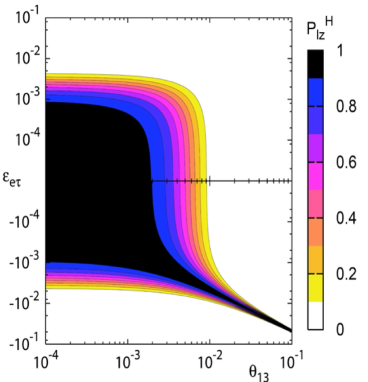
Figure 6.6: Landau-Zener jump probability isocontours at the $H$-resonance in terms of $\varepsilon_{e\tau}$ and $\theta_{13}$ for $\varepsilon_{\tau\tau}=10^{-4}$. Antineutrinos with energy $10$ MeV and inverted mass hierarchy has been assumed [21].

Turning to the case of the $L$-transition a similar expression can be obtained by rotating the original Hamiltonian by $U(\theta_{13})^{\dagger}U(\theta_{23})^{\dagger}$, as discussed in Chapter 2. However, in contrast to the case of the $H$-resonance, where the mixing angle $\theta_{13}$ is still unknown, in the case of the $L$-transition the angle $\theta_{12}$ has been shown by solar and reactor neutrino experiments to be large [45]. As a result, for the mass scale $\Delta_{\odot}$ this transition will always be adiabatic irrespective of the values of $\varepsilon_{\alpha\beta}$, and will affect only neutrinos.

Summarizing, we have obtained that in the absence of collective flavor transformations, the inclusion of NSI to the SN scenario mainly affects the evolution of neutrinos in two ways. Firstly, for sufficiently large diagonal NSI parameters, an internal resonance is induced. Secondly, the usual MSW $H$- and $L$-resonances are modified, essentially by a change in their position, but for some given values of $\theta_{13}$ and the NSI parameters also affecting the adiabaticity of the $H$-resonance.

6.3 Including the neutrino background

After discussing the genuine effects that NSI could induce in the evolution of SN neutrinos, let us now add to the picture the neutrino self-interactions. The important point to have in mind is that both ingredients may have drastic consequences in the same inner layers of the SN. It is therefore crucial to analyze the interplay between these two in principle coexisting effects.

6.3.1 Equations of motion

As it has already been discussed, in the presence of neutrino self-interactions it is convenient to make use of the density matrix formalism. We therefore recover the EOMs for neutrinos given in Eq. (4.1),

$${\rm i}\partial_{t}\varrho_{\bf p}=[{\sf H}_{\bf p},\varrho_{\bf p}]\,,$$ (6.30)

where $\varrho_{\bf p}$ and $\bar{\varrho}_{\bf p}$ represent the matrices of density describing each (anti)neutrino mode and the Hamiltonian was given in Eq. (4.2):

$${\sf H}_{\bf p}=\Omega_{\bf p}+{\sf V}+\sqrt{2}\,G_{\rm F}\!\int\!\frac{{\rm d}^{3}{\bf q}}{(2\pi)^{3}}\left(\varrho_{\bf q}-\bar{\varrho}_{\bf q}\right)(1-{\bf v}_{\bf q}\cdot{\bf v}_{\bf p})\,.$$ (6.31)

For antineutrinos the only difference is $\Omega_{\bf p}\to-\Omega_{\bf p}$.

The kinetic term will be determined by the mass and mixing parameters. We will use $\Delta m_{21}^{2}\equiv m_{2}^{2}-m_{1}^{2}=7.65\times 10^{-5}$ eV², $|\Delta m_{31}^{2}|\equiv|m_{3}^{2}-m_{1}^{2}|=2.40\times 10^{-3}$ eV² and $\sin^{2}\theta_{12}=0.3$. We consider also $\sin^{2}\theta_{13}=10^{-2}$ and three different values for $\theta_{23}$ in the allowed range at 3$\sigma$, $\sin^{2}\theta_{23}=$ 0.4, 0.5 and 0.6, because our results depend sensitively on $\theta_{23}$. Given the values of $\Delta m^{2}$ we obtain the two associated vacuum oscillation frequencies: $\omega_{\rm H}\equiv\Delta m^{2}_{31}/2E$ and $\omega_{\rm L}\equiv\Delta m^{2}_{21}/2E$, which in the case of neutrinos with $E=20$ MeV, lead to $\omega_{\rm H}=0.3$ km^-1 and $\omega_{\rm L}=0.01$ km^-1. In the top panel of Fig. 6.7 we represent $\omega_{\rm H}$ and $\omega_{L}$ for energies typical in SNe, between 5 MeV and 50 MeV, as yellow and light blue bands, respectively.

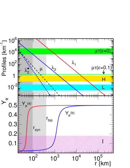
Figure 6.7: Top panel: Density profiles, $\lambda(r)$, for $\lambda_{0}=5\times 10^{9}$ km^-1 ($\lambda_{1}$) and $\lambda_{0}=4\times 10^{6}$ km^-1 ($\lambda_{2}$) in solid red and blue lines, respectively; $\lambda^{\star}(r)$ for $\lambda_{2}$ is shown in blue dotted lines; $\mu(r)$ for $\mu_{0}=7\times 10^{5}~{}$km^-1 in black dashed lines; the vacuum oscillation frequencies $\omega_{\rm H}$ (yellow band), $\omega_{L}$ (cyan band), and $\omega_{\mu\tau}$ for $\varepsilon_{\tau\tau}=0$ (green band), for energies between 5 and 50 MeV; $\omega^{\rm nsi}_{\mu\tau}$ for $\varepsilon_{\tau\tau}=0.1$ and $E=20$ MeV is also displayed (green solid line). The position of the synchronization and bipolar radii are also shown. Bottom: radial dependence of $Y_{e}$ for two set of parameters: $a=0.24,~{}b=0.165,~{}r_{0}=50~{}(1.2\times 10^{3})$ km, and $r_{s}=5~{}(3\times 10^{2})$ km, for $Y_{e}^{\rm a}~{}(Y_{e}^{\rm b})$. The horizontal magenta band represents the $Y_{e}^{I}$ leading to an internal $I$-resonance for $\varepsilon_{\tau\tau}\leq 0.1$ [22].

The only difference in Eq. (6.31) compared to the previous chapters resides in the matter potential, where we have to add the NSI contribution. Let us then concentrate the discussion in this term. As we have seen, the interaction of neutrinos with matter can be now split in two pieces:

$${\sf V}={\sf V}_{\rm std}+{\sf V}_{\rm nsi}~{}.$$ (6.32)

The first term, ${\sf V}_{\rm std}$, describes the standard interaction with matter and can be represented in the weak basis by

$${\sf V}_{\rm std}=\lambda(r){\rm diag}(Y_{e},0,Y_{\tau}^{\rm eff})\,,$$ (6.33)

with

$$\lambda(r)=\lambda_{0}\,\left(\frac{R_{\nu}}{r}\right)^{3}\,.$$ (6.34)

These expressions are equivalent to the ones in Eqs. (6.3) and (6.6) in units of km^-1. We have here left $Y_{e}$ outside the definition of $\lambda$ because of its special importance in the NSI effects. In the following we assume $R_{\nu}=10$ km. In the top panel of Fig. 6.7 we show two $\lambda(r)$ profiles for $\lambda_{0}=5\times 10^{9}$ km^-1 and $4\times 10^{6}$ km^-1 denoted by $\lambda_{1}$ and $\lambda_{2}$, corresponding to typical early and late time profiles, respectively, as illustrated in Fig. 5.1.

The first element in ${\sf V}_{\rm std}$ represents the charged current potential and is proportional to the electron fraction, $Y_{e}$. We parameterize $Y_{e}$ as in Eq. (6.7) with $a=0.24$ and $b=0.165$. The parameters $r_{0}$ and $r_{s}$ describe where the rise takes place and how steep it is, respectively. In the bottom panel of Fig. 6.7 we show two $Y_{e}(r)$ profiles for two different choices of these parameters. The radius where $\lambda(r)Y_{e}(r)$ crosses the horizontal bands $\omega_{\rm H}$ ($\omega_{\rm L}$) determines the well known $H$ ($L$) MSW resonances. For the $\lambda$ and $Y_{e}$ profiles shown in Fig. 6.7 and energies typical in SNe the position of both resonances $r^{\rm H}_{\rm res}$ and $r^{\rm L}_{\rm res}$ lie above $10^{3}$ km.

The other non-zero element in ${\sf V}_{\rm std}$ arises from radiative corrections to neutral-current $\nu_{\mu}$ and $\nu_{\tau}$ scattering, as discussed in Chapter 2. Although there are no $\mu$ nor $\tau$ leptons in normal matter, they appear as virtual states causing a shift $\Delta V_{\mu\tau}=\sqrt{2}\,G_{\rm F}Y_{\tau}^{\rm eff}n_{B}$ between $\nu_{\mu}$ and $\nu_{\tau}$ due to the difference in their masses, with $Y_{\tau}^{\rm eff}$ given in Eq. (5.1). In the top panel of Fig. 6.7 we show $\omega_{\mu\tau}\equiv\omega_{\rm H}/Y_{\tau}^{\rm eff}$ for energies between 5 and 50 MeV, as a green band. Analogously to the $H$- and $L$-resonances, the radius where $\lambda(r)\approx\omega_{\rm\mu\tau}$ defines the $\mu\tau$-resonance.

According to the description given in the previous section and in Chapter 3, the term in the Hamiltonian describing the non-standard neutrino interactions with a fermion $f$ can be expressed as,

$$({\sf V}_{\rm nsi})_{\alpha\beta}=\sum_{f=e,u,d}({\sf V}_{\rm nsi}^{f})_{\alpha\beta}=\sqrt{2}G_{F}N_{f}\varepsilon^{f}_{\alpha\beta}\,,$$ (6.35)

where $N_{f}$ represents the fermion $f$ number density. Again, we consider $\varepsilon^{f}_{\alpha\beta}\in\Re$, neglecting possible $CP$ violation in the new interactions, and take for $f$ the down-type quark. Therefore the NSI potential can be expressed as follows,

$$({\sf V}_{\rm nsi})_{\alpha\beta}=({\sf V}_{\rm nsi})_{\alpha\beta}=\varepsilon_{\alpha\beta}\lambda(r)(2-Y_{e})~{}.$$ (6.36)

In principle at least five of the six independent $\varepsilon_{\alpha\beta}$ parameters, after removing one of the diagonals, should be taken into account. Nevertheless, the exhaustive description developed in the previous section shows that all the physics involved can be described in terms of $\varepsilon^{\prime}_{\tau\tau}$ and $\varepsilon^{\prime}_{e\tau}$, which are just a suitable combination of $\varepsilon$’s. This motivates us to illustrate the interplay that could arise between collective effects and NSI by only considering two non-zero NSI parameters: $\varepsilon_{e\tau}$ and $\varepsilon_{\tau\tau}$, describing flavor-changing (FC) processes and non-universality (NU), respectively. Therefore the term in the Hamiltonian responsible for the interactions with matter can be written as

$${\sf V}=\lambda(r)(2-Y_{e})\left(\begin{array}[]{ccc}\frac{Y_{e}}{2-Y_{e}}&0&\varepsilon_{e\tau}\\ 0&0&0\\ \varepsilon_{e\tau}&0&\varepsilon_{\tau\tau}+\frac{Y_{\tau}^{\rm eff}}{2-Y_{e}}\end{array}\right)~{}.$$ (6.37)

This expresion is equivalent to Eq. (6.8), including the $\mu\tau$-term to the potential and considering only the desired NSI parameters. The range of values for the $\varepsilon$’s we consider is for the off-diagonal term $10^{-5}\lesssim|\varepsilon_{e\tau}|\lesssim{\rm few}\times 10^{-3}$. This prevents any significant NSI-induced reduction of the electron fraction $Y_{e}$ during the core collapse. For the diagonal term we assume $|\varepsilon_{\tau\tau}|\lesssim 0.1$, allowed by the current experimental constraints.

Finally, the third term in the Hamiltonian accounts for the collective flavor transformations induced by neutrino-neutrino interaction, and has been extensively described in Chapters 4 and 5. We consider the single-angle approximation by launching all neutrinos with $45^{\circ}$ relative to the radial direction. This approximation has been shown to be valid for realistic SN neutrino fluxes, provided that the neutrino density exceeds the electron density. The radial dependence of the neutrino-neutrino interaction strength can be explicitly written in such a system as

$$\mu(r)=\mu_{0}\frac{R_{\nu}^{4}}{r^{4}}\frac{1}{2-R_{\nu}^{2}/r^{2}}\approx\mu_{0}\frac{R_{\nu}^{4}}{2r^{4}}\,.$$ (6.38)

In the top panel of Fig. 6.7 we show the typical $\mu(r)$ profile we are using, with $\mu_{0}=7\times 10^{5}$ km^-1. One final property of SN neutrinos with important consequences for our study is the hierarchy of fluxes obtained in SN models. The typical conditions of the proto-neutron star lead to the following hierarchy of fluxes $F^{R_{\nu}}_{\nu_{e}}>F^{R_{\nu}}_{\bar{\nu}_{e}}>F^{R_{\nu}}_{\nu_{\mu}}=F^{R_{\nu}}_{\bar{\nu}_{\mu}}=F^{R_{\nu}}_{\nu_{\tau}}=F^{R_{\nu}}_{\bar{\nu}_{\tau}}$. As already discussed we express the lepton asymmetry with the parameter $\epsilon=(F^{R_{\nu}}_{\nu_{e}}-F^{R_{\nu}}_{\bar{\nu}_{e}})/(F^{R_{\nu}}_{\bar{\nu}_{e}}-F^{R_{\nu}}_{\bar{\nu}_{x}})$. Throughout the analysis we shall consider $\epsilon=0.25$. The equal parts of the fluxes drop out of the EOMs, so as initial condition we use in the monoenergetic case $F^{R}_{\nu_{\mu},\bar{\nu}_{\mu},\nu_{\tau},\bar{\nu}_{\tau}}=0$ and $F^{R}_{\nu_{e}}=(1+\epsilon)F^{R}_{\bar{\nu}_{e}}$.

6.3.2 Competition between NSI and collective effects

As it has already been discussed, in the absence of NSI and collective effects the neutrino propagation through the SN envelope is basically determined at the well-known MSW resonances. The $L$-resonance occurs always for neutrinos whereas the $H$-one takes place for (anti)neutrinos for (inverted) normal mass hierarchy. For our matter profiles and the values of $\theta_{12}$ and $\theta_{13}$ both resonances are adiabatic, see Fig. 2.7. Moreover both involve electron neutrino flavor and happen in the outer layers of the SN envelope, see top panel of Fig. 6.7.

In addition, the $\mu\tau$-resonance is also adiabatic, but occurs between the $\nu_{\mu}$ and $\nu_{\tau}$ or $\bar{\nu}_{\mu}$ and $\bar{\nu}_{\tau}$ depending on the neutrino mass hierarchy and the $\theta_{23}$ octant. However, when considering the neutrino self-interaction this resonance can also cause significant modifications of the overall $\nu_{e}$ and $\bar{\nu}_{e}$ survival probabilities [18]. According to the discussion in Sec. 6.3.1 the $\mu\tau$-resonance occurs at

$$r_{\mu\tau}\approx R_{\nu}~{}\left(\frac{\lambda_{0}Y_{\tau}^{\rm eff}}{\omega_{\rm H}}\right)^{1/3}=R_{\nu}~{}\left(\frac{\lambda_{0}}{\omega_{\rm\mu\tau}}\right)^{1/3}\,.$$ (6.39)

Due to the smallness of $Y_{\tau}^{\rm eff}$ the $\mu\tau$-resonance happens at deeper layers than the $H$- and $L$-resonances. In particular, for $\omega_{\rm H}=0.3$ km^-1, $Y_{e}=0.5$, and $\lambda_{0}=5\times 10^{9}$ km^-1 ($4\times 10^{6}$ km^-1) $r_{\mu\tau}=770$ km (71 km), see the intersection between the green band and the profiles $\lambda_{1}(r)$ and $\lambda_{2}(r)$ in the top panel of Fig. 6.7.

The consequence of the addition of an NSI term such as that of Eq. (6.36) is twofold. First, it will affect the MSW resonances. For the values assumed here the main effect on the $H$- and $L$-resonances will be just a slight shift in the resonance point, discussed in Sec. 6.2.2. The consequences for the $\mu\tau$-resonance can be more drastic. For sufficiently large values of $|\varepsilon_{\tau\tau}|$ a negative sign can change the resonance channel, from $\nu$ to $\bar{\nu}$ or viceversa, depending on the octant of $\theta_{23}$. On the other hand, it can significantly modify the position of the resonance. In the presence of NSI the $\mu\tau$-resonance happens at

$$r_{\mu\tau}\approx R_{\nu}~{}\left(\frac{\lambda_{0}Y_{\tau,{\rm nsi}}^{\rm eff}}{\omega_{\rm H}}\right)^{1/3}=R_{\nu}~{}\left(\frac{\lambda_{0}}{\omega_{\rm\mu\tau}^{\rm nsi}}\right)^{1/3}\,,$$ (6.40)

where we have defined

$$Y_{\tau,{\rm nsi}}^{\rm eff} \equiv Y_{\tau}^{\rm eff}+(2-Y_{e})\varepsilon_{\tau\tau}\,,$$ (6.41)

$$\omega^{\rm nsi}_{\mu\tau} \equiv \omega_{\rm H}/Y_{\tau,{\rm nsi}}^{\rm eff}\,.$$ (6.42)

In particular, for $|\varepsilon_{\tau\tau}|>Y_{\tau}^{\rm eff}/(2-Y_{e})$ the value of $\omega_{\mu\tau}^{\rm nsi}$ decreases, and therefore $r_{\mu\tau}$ is pushed outwards with respect to the standard case. In the top panel of Fig. 6.7 we show the value of $\omega^{\rm nsi}_{\mu\tau}$ in the presence of $\varepsilon_{\tau\tau}=0.1$ and $E=20$ MeV. For such a choice of parameters and the matter profile corresponding to $\lambda_{0}=4\times 10^{6}$ km^-1, we can see how the position of the $\mu\tau$-resonance moves out to a radius of $r_{\mu\tau}\approx 1.3\times 10^{3}$ km.

The second important consequence is that the new NSI terms can induce additional resonances in the inner layers, as described in Sec. 6.2. The condition required for this $I$-resonance to take place was given in Eq. (6.43) and can be written, for our simplified system, as

$$Y_{e}^{I}=\frac{2\varepsilon_{\tau\tau}}{1+\varepsilon_{\tau\tau}}~{}.$$ (6.43)

In the bottom panel of Fig. 6.7 we show as a horizontal band the range of $Y_{e}^{I}$ required for the $I$-resonance to take place for $\varepsilon_{\tau\tau}\leq 0.1$. For typical values of $Y_{e}$ one expects to have the $I$-resonance for $\varepsilon_{\tau\tau}\gtrsim 10^{-2}$. Moreover the $Y_{e}(r)$ and $|\varepsilon_{e\tau}|$ considered guarantee the adiabaticity.

At the same time, also in the internal region, the neutrino flux emerging from the SN core is so dense that, neutrino-neutrino refraction can cause nonlinear flavor oscillation phenomena. For the hierarchy of neutrino fluxes assumed the induced pair-wise flavor transformation occurs only in the case that the neutrino mass hierarchy is inverted. Collective flavor transformations start after the synchronization phase, where $\mu(r_{\rm syn})\approx 2\omega_{\rm H}/(1-\sqrt{1+\varepsilon})^{2}$, and extends a few hundred km in the so-called bipolar regime until $\mu(r_{\rm bip})\approx\omega_{\rm H}$. At larger radii $\mu(r)<\omega_{\rm H}$ and the neutrino self-interaction becomes negligible. For our chosen $\mu_{0}$, an excess $\nu_{e}$ flux of 25%, and $\omega_{\rm H}=0.3$ km^-1, we find a synchronization and bipolar radius of $r_{\rm syn}\simeq 100$ km and $r_{\rm bip}\simeq 330$ km, as indicated in Fig. 6.7 by dark and light vertical gray bands, respectively. One important consequence of this flavor transformation in the context of three neutrino flavors is its potential sensitivity to deviations of $\theta_{23}$ from maximal mixing. As discussed in Chapter 5, in the particular case that the $\mu\tau$-resonance takes place outside the synchronization radius the final $\nu_{e}$ and $\bar{\nu}_{e}$ survival probability depend crucially on the octant of $\theta_{23}$. In Sec. 5.6, we argued that this potential effect would most likely be suppressed by multi-angle decoherence induced by dense matter. Let us now analyze how the picture changes when considering NSI. According to Eqs. (6.40) and (4.15) the condition for this $\mu\tau$ effect to happen is given by

$$\lambda_{0}Y_{\tau,{\rm nsi}}^{\rm eff}\gtrsim\left(\frac{\sqrt{1+\epsilon}-1}{2}\right)^{3/2}\mu_{0}^{3/4}\omega_{\rm H}^{1/4}\sim 3\times 10^{2}~{}{\rm km}^{-1}\,.$$ (6.44)

Although this is a minimum requirement, the possibility to discern the $\theta_{23}$ octant becomes cleaner when the $\mu\tau$-resonance happens outside the bipolar radius, $r_{\mu\tau}>r_{\rm bip}$. The condition we obtain according to Eqs. (6.40) and (4.16) is, therefore,

$$\lambda_{0}Y_{\tau,{\rm nsi}}^{\rm eff}\gtrsim\left(\frac{\mu_{0}}{2}\right)^{3/4}\omega_{\rm H}^{1/4}\sim 10^{4}~{}{\rm km}^{-1}\,.$$ (6.45)

In the standard case this possibility only occurs for large density profiles, $\lambda_{0}\gtrsim 4\times 10^{8}$ km^-1, i.e. at early times. This situation would correspond to the $\lambda_{1}(r)$ profile in top panel of Fig. 6.7, but not to $\lambda_{2}(r)$. However the presence of NSI terms in the Hamiltonian may shift the $\mu\tau$-resonance to outer layers, making this condition more flexible. For instance, for $\varepsilon_{\tau\tau}=0.1$ the previous condition requires only $\lambda_{0}\gtrsim 1.3\times 10^{5}$ km^-1, see green solid line in the top panel of Fig. 6.7. Therefore the presence of NSI could keep the possibility to distinguish between the two $\theta_{23}$ octants for several seconds.

The self-induced flavor transformations however do not occur for arbitrarily large density profiles. If the electron density $n_{e}$ significantly exceeds the neutrino density $n_{\nu}$ in the conversion region they can be suppressed by matter. This is a consequence of neutrinos traveling on different trajectories when streaming from a source that is not point-like. This multi-angle matter effect can be neglected if in the collective region, prior to the synchronization radius, we have

$$\lambda^{\star}(r)\equiv Y_{e}(r)\lambda(r)\frac{R_{\nu}^{2}}{2r^{2}}\ll\mu(r)\,.$$ (6.46)

The limiting condition can be determined by imposing Eq. (6.46) at $r_{\rm syn}$. Taking into account Eqs. (6.34) and (6.38) we obtain

$$Y_{e}(r_{\rm syn})\lambda_{0}\frac{R_{\nu}}{r_{\rm syn}}\ll\mu_{0}\,.$$ (6.47)

Assuming $Y_{e}=0.5$ and $r_{\rm syn}=100$ km, this condition amounts to $\lambda_{0}\ll 1.4\times 10^{7}$ km^-1. In the top panel of Fig. 6.7 we show $\lambda_{2}^{\star}(r)$, corresponding to a $\lambda_{0}$ smaller than $\lambda_{0}\ll 1.4\times 10^{7}$ km^-1. The condition $\lambda_{2}^{\star}(r)\ll\mu(r)$ is then satisfied in the bipolar region, and collective effects are not matter suppressed. This is not the case of $\lambda_{1}(r)$. In the standard case the limiting $\lambda_{0}=1.4\times 10^{7}$ km^-1, above which multiangle matter effects suppress the collective effects, is though smaller than the minimum $\lambda_{0}=4\times 10^{8}$ km^-1 required for the $\mu\tau$ effect to be important. The situation could drastically change in the presence of NSI. Non-zero NSI diagonal parameters could help moving the $\mu\tau$ resonance out of the $r_{\rm syn}$ even for $\lambda_{0}$ smaller than $1.4\times 10^{7}$ km^-1. The consequence is that large enough $|\varepsilon_{\tau\tau}|$ would make the neutrino propagation through the SN envelope highly sensitive to the $\theta_{23}$ octant.

6.3.3 Classification of regimes

In this section we summarize all the information formerly introduced. Taking into account the conditions given in Eqs. (6.43), (6.44), (6.45), (6.46), and (6.47) we can roughly identify four different regimes of the neutrino propagation in terms of $\lambda_{0}$ and $\varepsilon_{\tau\tau}$. This scheme is displayed in Fig. 6.8.

To first approximation the four regions can be defined in terms of matter suppression (or not) of collective effects and presence (or not) of the internal $I$-resonance. Equation (6.47) is depicted as a horizontal solid line at $\lambda_{0}=1.4\times 10^{7}$ km^-1. For higher $\lambda_{0}$ matter suppresses collective effects whereas for smaller densities collective effects are present. For intermediate values, $\lambda^{\star}(r)\sim\mu(r)$, there would be a matter induced decoherence [20]. To make the discussion as simple as possible we will only consider the extreme cases. On the other hand the vertical dashed line at $\varepsilon_{\tau\tau}=10^{-2}$ indicates the presence (right) or absence (left) of the NSI-induced $I$-resonance.

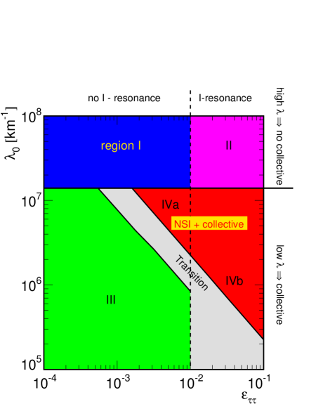
Figure 6.8: Different regimes of the neutrino propagation depending on the value of $\lambda_{0}$ and $\varepsilon_{\tau\tau}$, as described in the text [22].

This simple scheme becomes further complicated if one adds the possibility that the $\mu\tau$-resonance lies outside the bipolar region. In the next subsections we analyze in detail the different possibilities.

A) Region I
On the upper left corner we have the region I, defined by $\lambda_{0}\gtrsim 1.4\times 10^{7}$ km^-1 and $\varepsilon_{\tau\tau}\lesssim 10^{-2}$. According to the previous discussion, this range of parameters leads to no collective effects, since they are suppressed by matter, and no $I$-resonance. Assuming that the $L$- and $H$-resonances are adiabatic the $\nu_{e}$ and $\bar{\nu}_{e}$ survival probability is then only fixed by the mass hierarchy. The NSI terms will lead at most to a small shift in its position.

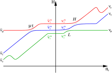
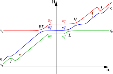
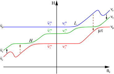
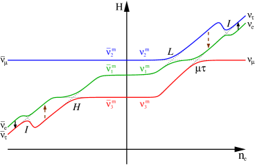
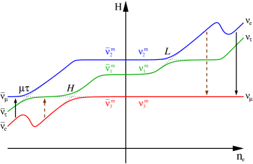
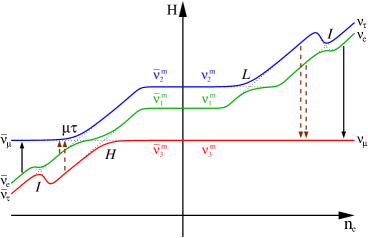
Figure 6.9: Level crossings in the absence (left) and presence (right) of $I$-resonance for normal (top), and inverted mass hierarchy for $\sin^{2}\theta_{23}=0.4$ (middle), and $\sin^{2}\theta_{23}=0.6$ (bottom). The dashed and solid arrows in the middle and bottom indicate the pair transformations due to collective effects happening after (dashed) or before (solid) the $\mu\tau$-resonance [22].

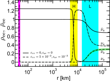
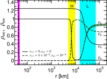
Figure 6.10: Radial dependence of $\rho_{ee}$ and $\bar{\rho}_{ee}$ corresponding to regions I (solid) and II (dashed) in Fig. 6.8. Left panel represents normal mass hierarchy and right panel inverted mass hierarchy. We assume $\lambda_{0}=10^{8}$ km^-1, $\omega_{\rm H}=0.3$ km^-1, and $\sin^{2}\theta_{23}=0.5$. Vertical bands indicate regions where resonances take place [22].

In Fig. 6.9 we show the well known level crossing schemes for normal (top), and inverted mass hierarchy for $\sin^{2}\theta_{23}<\pi/4$ (middle), and $\sin^{2}\theta_{23}>\pi/4$ (bottom), with (left column) and without (right column) $I$-resonance, where we have now added arrows representing the transitions caused by the collective effects. The arrows must therefore be ignored when these are not present. In the normal hierarchy case $\nu_{e}$ and $\bar{\nu}_{e}$ leave the SN as $\nu_{3}$ and $\bar{\nu}_{1}$, whereas for inverted mass hierarchy they escape as $\nu_{2}$ and $\bar{\nu}_{3}$ for any octant. The survival probabilities can then be written as $P(\nu_{e}\rightarrow\nu_{e})\approx\sin^{2}\theta_{13}~{}(\sin^{2}\theta_{12})$ and $P(\bar{\nu}_{e}\rightarrow\bar{\nu}_{e})=\cos^{2}\theta_{12}~{}(\sin^{2}\theta_{13})$ for normal (inverted) mass hierarchy. Figure 6.10 represents in solid lines the radial evolution of $\rho_{ee}$ and $\bar{\rho}_{ee}$ assuming $\lambda_{0}=10^{8}$ km^-1, $\omega_{\rm H}=0.3$ km^-1, $\sin^{2}\theta_{23}=0.5$, and $\epsilon=0.25$. The vertical bands indicate where the resonance conversions take place. In order to perform the plot we have artificially set $\mu_{0}=0$. We want to recall here that both $\rho_{ee}$ and $\bar{\rho}_{ee}$ are normalized to the $\bar{\nu}_{e}$ flux, and therefore, while $\bar{\rho}_{ee}$ corresponds directly to $\bar{\nu}_{e}$ survival probability, $\rho_{ee}$ must be corrected by a factor $(1+\epsilon)$ in order to obtain the corresponding survival probability, $\rho_{ee}=P(\nu_{e}\rightarrow\nu_{e})(1+\epsilon)$. This region, therefore, corresponds to the physics of oscillation discussed in Chapter 2.
B) Region II
The region II, on the upper right corner, is defined by $\lambda_{0}\gtrsim 1.4\times 10^{7}$ km^-1 and $\varepsilon_{\tau\tau}\gtrsim 10^{-2}$. As in I the matter density is so high that prevents neutrinos from undergoing collective effects. However, the values of the diagonal NSI terms in this region are large enough to fulfill Eq. (6.43), causing the $I$-resonance to appear. In contrast to the previous case $\nu_{e}$ and $\bar{\nu}_{e}$ are now created as $\nu_{2}^{\rm m}$ ($\nu_{1}^{\rm m}$) and $\bar{\nu}_{2}^{\rm m}$ ($\bar{\nu}_{1}^{\rm m}$) for normal (inverted) mass hierarchy, cross adiabatically all resonances and leave the SN as $\nu_{2}$ ($\nu_{1}$) and $\bar{\nu}_{2}$ ($\bar{\nu}_{1}$) for normal (inverted) mass hierarchy [21]. The survival probabilities are now $P(\nu_{e}\rightarrow\nu_{e})=P(\bar{\nu}_{e}\rightarrow\bar{\nu}_{e})\approx\sin^{2}\theta_{12}~{}(\cos^{2}\theta_{12})$ for normal (inverted) mass hierarchy. The black dashed lines in Fig. 6.10 show the expected radial evolution of $\rho_{ee}$ and $\bar{\rho}_{ee}$, respectively, when neutrinos and antineutrinos undergo an adiabatic $I$-resonance. The green band represents the presence of phases. As for region I, we have made the calculation assuming $\mu_{0}=0$. However, we have analyzed the single energy and multiangle case within two-flavor framework for the range of parameters here discussed, and have verified that collective effects are indeed suppressed and the $I$-resonance is present for both normal and inverted hierarchies. That means that the behavior in region II corresponds indeed to the case discussed in Sec. 6.2.
C) Region III
Let us now consider the lower part of Fig. 6.8, i.e. when $\lambda_{0}\lesssim 1.4\times 10^{7}$ km^-1. The main characteristic of this scenario is the presence of collective effects. As it was discussed in Ref. [18], and here reviewed, these in turn depend on the relative position of the $\mu\tau$-resonance with respect to the synchronization and bipolar radius. We can then distinguish two different regimes: On the bottom left corner we define the region III by the condition $r_{\mu\tau}\lesssim r_{\rm syn}$, and on the bottom right corner we have region IV defined by $r_{\mu\tau}\gtrsim r_{\rm bip}$. In the middle of both there is a transition region where $r_{\rm bip}\gtrsim r_{\mu\tau}\gtrsim r_{\rm syn}$, which we will not consider here.

Let us now discuss region III. According to Eq. (6.45) this range of parameters satisfies the condition

$$\lambda_{0}[Y_{\tau}^{\rm eff}+(2-Y_{e})\varepsilon_{\tau\tau}]\lesssim 10^{4}~{}{\rm km}^{-1}\,,$$ (6.48)

which, for $Y_{e}=0.5$, roughly amounts to $\lambda_{0}\varepsilon_{\tau\tau}\lesssim 7.3\times 10^{3}$ km^-1, see Fig. 6.8. This situation can be reduced to the standard two-flavor scenario previously analyzed in this thesis. In order to better understand the consequences of collective effects it is convenient to recall that the impact of ordinary matter can be transformed away by going into a rotating reference frame for the polarization vectors. Collective conversions proceed in the same way as they would in vacuum, except that the effective mixing angle is reduced. The connection between flavor $\nu_{\alpha}$ and vacuum $\nu_{i}$ eigenstates can be done in the level crossing schemes by propagating the former ones from regions at high density to vacuum crossing all resonances non-adiabatically. The initial states $\nu_{e}$ and $\bar{\nu}_{e}$ can therefore be identified with $\nu_{1}$ and $\bar{\nu}_{1}$, respectively. If the neutrino mass hierarchy is normal, we begin in the lowest-lying state and nothing happens. The situation is then similar to that in region I, i.e. without collective effects, see left panel of Fig. 6.10. However in the case of inverted mass hierarchy both $\nu_{1}$ and $\bar{\nu}_{1}$ correspond to the intermediate state. The effect of the self-interaction is to drive them to the lowest-lying states, which in this case are $\nu_{3}$ and $\bar{\nu}_{3}$. This is shown by dashed arrows in the middle and bottom left panels of Fig. 6.9. In the case of $\nu_{e}$ a fraction equal to $\epsilon F_{\bar{\nu}_{e}}$ is not transformed and stays in $\nu_{2}^{\rm m}$ and evolves as in the absence of neutrino-neutrino interactions, i.e. adiabatically through the $L$-resonance. The rest of $\nu_{e}$ are transformed to $\nu_{3}^{\rm m}$. As a consequence, the final $\nu_{e}$ flux, normalized to the initial $\bar{\nu}_{e}$ one, is expected to be approximately $\rho^{\rm final}_{ee}=\epsilon\sin^{2}\theta_{12}+\sin^{2}\theta_{13}\simeq 0.08$. On the other hand, after the pair transformation $\bar{\nu}_{e}$ cross the $H$-resonance adiabatically and leave the star as $\nu_{1}$, leading to a final normalized flux of approximately $\bar{\rho}^{\rm final}_{ee}=\cos^{2}\theta_{12}\simeq 0.7$. This can be seen in Fig. 6.11, where we show in solid lines the radial evolution of $\nu_{e}$ and $\bar{\nu}_{e}$ for inverted mass hierarchy assuming $\lambda_{0}=4\times 10^{6}$ km^-1, $\omega_{\rm H}=0.3$ km^-1, and $\sin^{2}\theta_{23}=0.4$ (left) and 0.6 (right).

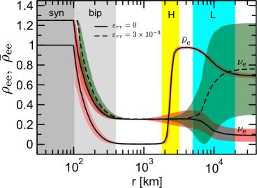
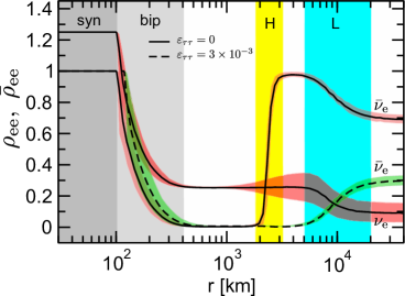
Figure 6.11: Radial dependence of $\rho_{ee}$ and $\bar{\rho}_{ee}$ for region III with $\varepsilon_{\tau\tau}=0$ (solid) and IVa (dashed) with $\varepsilon_{\tau\tau}=3\times 10^{-3}$ for inverted mass hierarchy, and $\sin^{2}\theta_{23}=0.4~{}(0.6)$ in the left (right panel). In both cases $\lambda_{0}=4\times 10^{6}$ km^-1 and $\varepsilon_{e\tau}=0$. The bands around the lines represent modulations. Vertical gray bands stand for synchronized (dark) and bipolar (light) regime. Resonance regions are also displayed [22].

As can be seen in the figure, the result is independent of the $\theta_{23}$ octant. The evolution of neutrinos in this region of parameters therefore corresponds to the description given in Chapters 4 and 5.
D) Region IV
Finally, neutrinos with parameters in the right bottom corner (region IV) will feel both collective and NSI effects. This region of parameters is defined by the condition that the $\mu\tau$-resonance lies outside the bipolar region. According to Eq. (6.45) this amounts to

$$\lambda_{0}[Y_{\tau}^{\rm eff}+(2-Y_{e})\varepsilon_{\tau\tau}]\gtrsim 2\times 10^{4}~{}{\rm km}^{-1}\,.$$ (6.49)

As discussed above, for the standard case and $Y_{e}=0.5$ this is satisfied for $\lambda_{0}\gtrsim 7\times 10^{8}$ km^-1, which implies a strong matter suppression of the collective effects, see Fig. 6.8. However, if NSI diagonal parameters are of the order of $|\varepsilon_{\tau\tau}|\gtrsim 5.3\times 10^{3}/\lambda_{0}~{}({\rm km}^{-1})$ then one can avoid the matter suppression condition. Therefore the first NSI effect is to increase the value of $Y_{\tau,{\rm nsi}}^{\rm eff}$ so that the $\lambda_{0}$ required to have the $\mu\tau$-resonance outside $r_{\rm bip}$ is still consistent with the presence of collective effects. On top of that, if $\varepsilon_{\tau\tau}$ is of the order of a few % the condition given in Eq. (6.43) is fulfilled for the typical values of $Y_{e}$ found in SNe. Thus, in the region IV we can distinguish two subsets of parameters denoted by IVa and IVb defined by the absence or presence of the $I$-resonance, respectively. For defineteness we set the boundary at $\varepsilon_{\tau\tau}=10^{-2}$.

Let us first consider the IVa region. Depending on $\lambda_{0}$, i.e. on the instant considered, this range of parameters implies values of $|\varepsilon_{\tau\tau}|$ from $10^{-3}$ to $\sim 10^{-2}$. Although these values are not high enough to induce the $I$-resonance they are sufficiently large to push the $\mu\tau$-resonance outside the bipolar region. The situation is therefore analogous to the one described in Chapter 5. That means a flavor pair transformation $\nu_{e}\bar{\nu}_{e}\rightarrow\nu_{x}\bar{\nu}_{x}$ due to collective effects only for inverted neutrino mass hierarchy, like in region III. However, the final matter eigenstates depend on the $\theta_{23}$ octant. In the middle left panel of Fig. 6.9 we show with solid lines the pair conversion for $\theta_{23}$ in the first octant. In terms of matter eigenstates, $\nu_{e}$ and $\bar{\nu}_{e}$ are transformed into $\nu_{1}^{\rm m}$ and $\bar{\nu}_{1}^{\rm m}$, respectively. The presence of the $\mu\tau$-resonance in the neutrino channel leads to a difference of $\nu_{e}$ with respect to region III. In the left panel of Fig. 6.11 we show with dashed lines the evolution of $\nu_{e}$ as function of the distance, for $\varepsilon_{\tau\tau}=3\times 10^{-3}$ and $\sin^{2}\theta_{23}=0.4$. In the collective bipolar conversions, the excess $\epsilon$ of $\nu_{e}$ over $\bar{\nu}_{e}$ remains as $\nu_{2}^{\rm m}$ whereas the rest will be transformed to $\nu_{1}^{\rm m}$. As a consequence, the original $\nu_{e}$ flux leaving the star can be written as $\rho^{\rm final}_{ee}=\varepsilon\sin^{2}\theta_{12}+\cos^{2}\theta_{12}$, which in our particular case amounts to roughly 0.75. If $\theta_{23}$ belongs to the second octant the $\mu\tau$-resonance takes place in the antineutrino channel, see bottom left panel of Fig. 6.9. The pair $\nu_{e}$ and $\bar{\nu}_{e}$ is driven to the lowest-lying states, which in this case are $\nu_{3}^{\rm m}$ and $\bar{\nu}_{2}^{\rm m}$, for neutrinos and antineutrinos, respectively. Therefore, for $\nu_{e}$ the situation is completely analogous to that in region III, whereas $\bar{\nu}_{e}$ leave the star as $\bar{\nu}_{2}$. In the right panel of Fig. 6.11 it is displayed with dashed lines the radial evolution of $\bar{\nu}_{e}$ for $\varepsilon_{\tau\tau}=3\times 10^{-3}$ and $\sin^{2}\theta_{23}=0.6$. It is remarkable that neither $\nu_{e}$ nor $\bar{\nu}_{e}$ undergo the H resonance, and therefore are blind to the possible effect of the outwards propagating shock wave [70, 71, 66].

It is important to notice that the same effect observed for the different octants of $\theta_{23}$ can be obtained by fixing the octant and changing the sign of $\varepsilon_{\tau\tau}$. This can be easily understood if we study the $\mu\tau$-resonance condition,

$$\lambda(r)[Y^{\rm eff}_{\tau}+(2-Y_{e})\varepsilon_{\tau\tau}]\simeq-\omega_{\rm H}\cos^{2}{\theta_{13}}\cos{2\theta_{23}}\,,$$ (6.50)

where we have neglected subleading solar terms. This condition dictates the channel where the resonance takes place. In the standard case this only determined by the hierarchy of neutrino masses and the octant of $\theta_{23}$. In the presence of NSI, though, the sign of left-hand side of the equation depends on that of $\varepsilon_{\tau\tau}$, what therefore affects directly to the resonance condition. As a consequence, the same result of Fig. 6.11 is obtained by changing the sign of $\varepsilon_{\tau\tau}$ and the octant of $\theta_{23}$, i.e. $\varepsilon_{\tau\tau}=-3\times 10^{-3}$ and second octant for the panel on the left and first octant in the right panel. The bottom line is that, in the presence of NSI parameters such that $|\varepsilon_{\tau\tau}|\gtrsim$ a few$\times 10^{-4}$, SN neutrinos are sensitive to the octant of $\theta_{23}$, the absolute value of the NSI diagonal parameter as well as its sign. In this region, the propagation of neutrinos is analogous to the one described in Chapter 5.

Finally, for higher values of the NSI diagonal parameters, $\varepsilon_{\tau\tau}\gtrsim 10^{-2}$ (region IVb), the internal $I$-resonance will arise. In this case one has to analyze the interplay between collective effects and the $I$-resonance. This is discussed in the next section.

6.3.4 Collective effects and NSI-induced $I$-resonance

In this section we analyze region IVb, defined by $\lambda_{0}\lesssim 1.4\times 10^{7}$ km^-1 and $\varepsilon_{\tau\tau}\gtrsim 10^{-2}$, where both an adiabatic $I$-resonance and collective effects are present. If the $I$-resonance is not adiabatic then neutrinos within region IVb evolve exactly as in IVa.

As can be inferred from Fig. 6.7, one of the main features of this scenario is that both effects happen nearly in the same region, namely the deepest layers right above the neutrino sphere. That means that the final result will also depend on the relative position between the bipolar region and the location of the $I$-resonance. Schematically two extreme scenarios can be identified. In one case the rise in the $Y_{e}$, and consequently the $I$-resonance, takes place before the bipolar conversion region, see $Y_{e}^{\rm a}$ in the bottom panel of Fig. 6.7. In the second scenario one has first the bipolar conversion and then neutrinos traverse the $I$-resonance, see $Y_{e}^{\rm b}$ in the bottom panel of Fig. 6.7.
A) First NSI $I$-resonance
Let us analyze here the case where the $I$-resonance happens in deeper layers than collective effects. This situation corresponds to the $Y_{e}^{\rm a}$ in the bottom panel of Fig. 6.7 and, according to SN numerical simulations it is the most likely situation.

The main consequence of an $I$-resonance in the most inner layers, right after the neutrino sphere, is an inversion of the neutrino fluxes entering the bipolar region. For the initial flux pattern assumed this implies the following new pattern after the $I$-resonance: $F_{\nu_{e}}=F_{\bar{\nu}_{e}}=0$, $F_{\nu_{\tau}}=1+\epsilon$, and $F_{\bar{\nu}_{\tau}}=1$ normalized to $F_{\bar{\nu}_{e}}$. Contrarily to the standard case, under this condition collective effects arise in the case of normal mass hierarchy.

This can be understood using the pendulum analogy in the corresponding reduced two flavor scenario, and keeping in mind that the bipolar conversion drives the neutrinos to the lowest-lying states. In the normal hierarchy the system is already created near the minimum of the potential. Thus, in absence of the $I$-resonance collective effects are not present. However once an adiabatic $I$-resonance is switched on the neutrino flavor is swapped and the system is driven to the maximum of the potential. In this situation bipolar effects act leading $\nu_{e}$ and $\bar{\nu}_{e}$ back to the lowest-lying states, i.e. to $\nu_{3}^{\rm m}$ and $\bar{\nu}_{1}^{\rm m}$, respectively. See dashed arrows in the top right panel of Fig. 6.9. As a consequence both the $I$-resonance and the induced collective effects basically cancel each other. In the left panel of Fig. 6.12 we show the radial evolution of $\nu_{e}$ and $\bar{\nu}_{e}$. This cancellation between the $I$-resonance and collective effects is complete for $\bar{\nu}_{e}$, which leave as $\bar{\nu}_{1}^{\rm m}$, but not for $\nu_{e}$: its excess $\epsilon$ over $\bar{\nu}_{e}$ is not transformed back to $\nu_{3}^{\rm m}$ but remains as $\nu_{2}^{\rm m}$. Therefore in the case of a monochromatic neutrino flux we obtain $\rho^{\rm final}_{ee}=\epsilon\sin^{2}\theta_{12}+\sin^{2}\theta_{13}\approx 0.08$, see left panel of Fig. 6.12, instead of simply $\sin^{2}\theta_{13}=10^{-2}$ as in left panel of Fig. 6.10. This result does not depend on the $\theta_{23}$ octant since the collective effects bring the $\nu_{e}\bar{\nu}_{e}$ pair to $\nu_{3}^{\rm m}\bar{\nu}_{1}^{\rm m}$ in both cases. Hence, by comparing the left panels of Figs. 6.10 and 6.12 one realizes that, except for the excess $\epsilon$, the situation for normal mass hierarchy is basically the same as in regions I, III, and IVa.

While this is true in the monoenergetic case a specific signature can be observed if we do not restrict ourselves to that case but consider the whole energy spectrum. The left panel of Fig. 6.13 displays the $\nu_{e}$ and $\nu_{x}$ fluxes at the neutrino sphere, $f^{\rm R}_{\nu_{e}}$ and $f^{\rm R}_{\nu_{x}}$. We have assumed the parameterization given in Ref. [201],

$$f^{R_{\nu}}_{\nu_{\alpha}}(E)=C_{\nu_{\alpha}}\left(\frac{E}{\langle{E_{\nu_{\alpha}}}\rangle}\right)^{\beta_{\nu_{\alpha}}-1}\exp\left(-\beta_{\nu_{\alpha}}\frac{E}{\langle{E_{\nu_{\alpha}}}\rangle}\right)\,,$$ (6.51)

with $\langle E_{\nu_{e}}\rangle=12$ MeV, $\langle E_{\nu_{e}}\rangle=15$ MeV, $\langle E_{\nu_{x}}\rangle=18$ MeV, $\beta_{\nu_{e}}=5,~{}\beta_{\bar{\nu}_{e}}=4.5$ and $\beta_{\nu_{x}}=4$. The normalization $C_{\nu_{\alpha}}$ has been chosen such that $F^{R_{\nu}}_{\bar{\nu}_{e}}\equiv\int f^{R_{\nu}}_{\bar{\nu}_{e}}(E){\rm d}E=1$, $F^{R_{\nu}}_{\nu_{e}}=1+\kappa\epsilon$ and $F^{R_{\nu}}_{\nu_{x}}=1-\kappa$, with $\kappa=0.15$.

As in standard case for inverted mass hierarchy, the excess $\epsilon$ of $\nu_{e}$ translates into a spectral split. However, in contrast to the standard case this excess concentrates at high energies. In the right panel of Fig. 6.13 we show the $\nu_{e}$ fluxes after the bipolar region. In solid dark red lines is represented the case under discussion: normal mass hierarchy in region IVb. By comparing the two panels one sees how the conversion $\nu_{e}\rightarrow\nu_{x}$ takes place only at low energies. This is exactly the contrary to what occurs for the standard case (inverted mass hierarchy in region III), shown as solid light red lines, where the untransformed flux concentrates at low energies. For completeness we show also the other cases. In the region of parameters I, III and IVa there is neither collective effects nor $I$-resonance for normal hierarchy, then the fluxes after the bipolar region coincide with the initial ones, $f_{\nu_{e}}=f_{\nu_{e}}^{R_{\nu}}$ and $f_{\nu_{x}}=f_{\nu_{x}}^{R_{\nu}}$. In region II, the $I$-resonance implies a complete conversion $\nu_{e}\rightarrow\nu_{x}$, what leads to a spectral swap, $f_{\nu_{e}}=f_{\nu_{x}}^{R_{\nu}}$ and $f_{\nu_{x}}=f_{\nu_{e}}^{R_{\nu}}$.

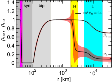
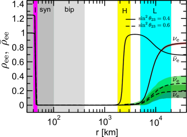
Figure 6.12: Same as Fig. 6.10 for region IVb, for normal (left panel) and inverted (right panel) mass hierarchy. In the left panel it is shown the case $\sin^{2}\theta_{23}=0.4$, while in the right panel the case $\sin^{2}\theta_{23}=0.6$ is also displayed. In both cases $\lambda_{0}=4\times 10^{6}$ km^-1 and $\varepsilon_{\tau\tau}=5\times 10^{-2}$ and $\varepsilon_{e\tau}=10^{-3}$. The $I$-resonance is assumed to occur before the collective effects [22].

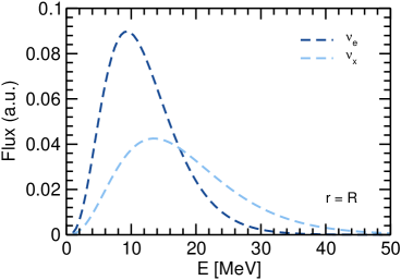
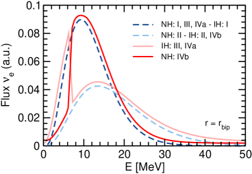
Figure 6.13: Left: $\nu_{e}$ and $\nu_{x}$ fluxes as emitted at the neutrino sphere. Right: $\nu_{e}$ flux after the bipolar region for different cases. In the region IVb it is assumed that the $I$-resonance occurs before than the bipolar conversion [22].

The case of inverted mass hierarchy is more subtle. According to the previous discussion one would expect no collective effects after neutrinos traverse the $I$-resonance. The system starts its evolution near the maximum of the potential and, in the absence of NSI, the bipolar conversions would take it to the minimum. What the $I$-resonance is doing in this language by swapping the flavor eigenstates is to take the system to the minimum of the potential before any collective effects can arise. The new stable situation prevents bipolar conversions, leaving the system unchanged until the outer resonances are reached. And this is indeed what happens if $\theta_{23}$ lies in the first octant, see middle right panel of Fig. 6.9. After the $I$-resonance the original $\nu_{e}$ and $\bar{\nu}_{e}$ are already in the state of “minimum energy”, which in this case corresponds to $\nu_{1}^{\rm m}$ and $\bar{\nu}_{1}^{\rm m}$ ($\nu_{3}$ and $\bar{\nu}_{3}$ after rotating the matter term away). Hence no collective effects take place, and $\nu_{e}$ and $\bar{\nu}_{e}$ leave the star as $\nu_{1}$ and $\bar{\nu}_{1}$, respectively, see solid lines in the right panel of Fig. 6.12.

However if $\theta_{23}$ belongs to the second octant things are different. The $I$-resonance drives now $\nu_{e}$ and $\bar{\nu}_{e}$ to the states of “maximum energy”, $\nu_{2}$ and $\bar{\nu}_{2}$ after rotating the matter term away, see bottom right panel of Fig. 6.9. That means, that in contrast to the first-octant case, when the neutrinos traverse the bipolar regime they will be driven to the lowest-lying states, i.e. $\nu_{2}\bar{\nu}_{2}\rightarrow\nu_{3}\bar{\nu}_{3}$, see dashed arrows in the figure. In terms of matter eigenstates that means a pair conversion from $\nu_{1}^{\rm m}\bar{\nu}_{1}^{\rm m}$ into $\nu_{3}^{\rm m}\bar{\nu}_{2}^{\rm m}$. In the right panel of Fig. 6.12 we show in dashed lines the evolution of $\nu_{e}$ and $\bar{\nu}_{e}$ as function of distance for $\sin^{2}\theta_{23}=0.6$. The bipolar conversion can not be seen as it occurs between $\nu_{1}^{\rm m}\bar{\nu}_{1}^{\rm m}$ and $\nu_{3}^{\rm m}\bar{\nu}_{2}^{\rm m}$, while $\nu_{e}$ and $\bar{\nu}_{e}$ coincide in that region with $\nu_{3}^{\rm m}$ and $\bar{\nu}_{2}^{\rm m}$, respectively. At the end, $\bar{\nu}_{e}$ leave the SN as $\bar{\nu}_{2}$, see right panel of Fig. 6.12. In the case of $\nu_{e}$ the excess $\epsilon$ over $\bar{\nu}_{e}$ remains as $\nu_{1}^{\rm m}$ whereas the rest is transformed to $\nu_{3}^{\rm m}$. Therefore for a monoenergetic flux we find $\rho^{\rm final}_{ee}=\epsilon\cos^{2}\theta_{12}+\sin^{2}\theta_{13}\approx 0.2$. By comparing the right panel of Figs. 6.11 and 6.12 one realizes that this case is analogous to IVa. Since the collective effects do not affect $\nu_{e}$ and $\bar{\nu}_{e}$ directly, considering neutrinos with an energy spectrum, one expects simply a complete swap of spectra, $f_{\nu_{e}}=f_{\nu_{x}}^{R}$ and $f_{\nu_{x}}=f_{\nu_{e}}^{R}$, like in scenario II, see right panel of Fig. 6.13.

The final conclusion is that the propagation of neutrinos with parameters in region IV is practically independent of the presence (IVb) or not (IVa) of the $I$-resonance. The main consequence of the $I$-resonance is to remove the spectral split expected in the inverted mass hierarchy, and create an inverted spectral split for $\nu_{e}$ for normal mass hierarchy.
B) First Collective
For completeness we have also considered the possibility that the bipolar conversion takes place before neutrinos traverse the $I$-resonance. This situation corresponds schematically to the $Y_{e}^{\rm b}$ profile in the bottom panel of Fig. 6.7.

The case of normal mass hierarchy is completely analogous to the one of region II, that is, absence of collective effects and $I$-resonance. The $\nu_{e}$ and $\bar{\nu}_{e}$ are created as $\nu_{2}^{\rm m}$ and $\bar{\nu}_{2}^{\rm m}$, respectively. Therefore, if all resonances involved, $I,~{}\mu\tau,~{}H,$ and $L$, are adiabatic then they leave the SN as $\nu_{2}$ and $\bar{\nu}_{2}$, respectively, see left panel of Fig. 6.14. The result is identical to the one shown with dashed lines in the left panel of Fig. 6.10.

The situation with inverted mass hierarchy depends significantly on the $\theta_{23}$ octant. Rotating the matter term away $\nu_{e}$ and $\bar{\nu}_{e}$ are created as the intermediate states $\nu_{1}$ and $\bar{\nu}_{1}$. Collective effects drive them to the lowest-lying states $\nu_{3}$ and $\bar{\nu}_{3}$. However the corresponding matter eigenstates are different depending on whether $\theta_{23}$ belongs to the first or to the second octant. In the first case, most of $\nu_{e}$ and $\bar{\nu}_{e}$ end up as $\nu_{2}^{\rm m}$ and $\bar{\nu}_{3}^{\rm m}$ before crossing the $I$-resonance, see solid arrows in the middle right panel of Fig. 6.9. The excess $\epsilon$ of $\nu_{e}$ stays as $\nu_{1}^{\rm m}$. As a consequence, the final $\nu_{e}$ and $\bar{\nu}_{e}$ fluxes, normalized to the initial $\bar{\nu}_{e}$ one, are $\rho^{\rm final}_{ee}=\epsilon\cos^{2}\theta_{12}+\sin^{2}\theta_{12}$ and $\bar{\rho}^{\rm final}_{ee}=\sin^{2}\theta_{13}$, respectively. See solid lines in the right panel of Fig. 6.14. Except for the excess $\epsilon$ in $\nu_{e}$ the net result is a cancellation of the collective effects and the $I$-resonance, leading to a similar result as in region I (solid lines in right panel of Fig. 6.10). Qualitatively, the main difference shows up in the $\nu_{e}$ spectrum. The initial collective effects induces a “standard” spectral split, i.e. spectral swap only at high energies. Nevertheless, as neutrinos cross the $I$-resonance this split turns into an inverse one, with a swap at low energies. The final result right after the $I$-resonance is analogous to the case of normal mass hierarchy and the $I$-resonance happening first, displayed with dark red solid lines in the right panel of Fig. 6.13.

If $\theta_{23}$ lies in the second octant then most of $\nu_{e}$ and $\bar{\nu}_{e}$ end up as $\nu_{3}^{\rm m}$ and $\bar{\nu}_{2}^{\rm m}$. As can be seen in the solid lines in the bottom right panel of Fig. 6.9 these neutrinos will not traverse the $I$-resonance, except the excess $\epsilon$ of $\nu_{e}$, which stays as $\nu_{1}^{\rm m}$. These neutrinos will be basically blind to the $I$-, $H$-, and $L$-resonances. The final fluxes will be therefore $\rho^{\rm final}_{ee}=\sin^{2}\theta_{13}+\epsilon\cos^{2}\theta_{12}$ and $\bar{\rho}^{\rm final}_{ee}=\sin^{2}\theta_{12}$. This case is represented with dashed lines in the bottom right panel of Fig. 6.14. In the end the final evolution turns out to be similar to that in region IVb.

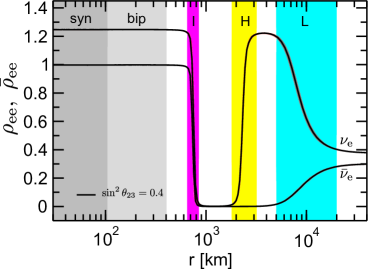
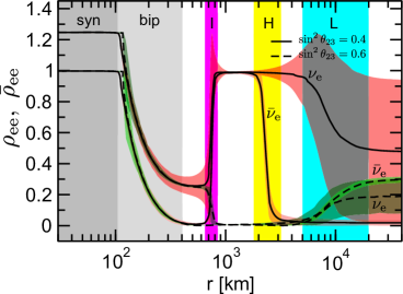
Figure 6.14: Same as Fig. 6.12 but assuming that the collective effects take place before the $I$-resonance [22].

6.3.5 Discussion

In the previous sections we have studied the consequences of NSI on the neutrino propagation through the SN envelope taking into account the presence of a neutrino background. We have analyzed the different situations in terms of the non-universal NSI parameter $\varepsilon_{\tau\tau}$ and the density at the neutrino sphere $\lambda_{0}$. Depending on their values we were able to identify four extreme regions of the parameters where the evolution of the neutrinos have a specific pattern.

In a realistic situation, though, we expect to find a combination of these situations depending on the instant considered. As mentioned in Sec. 6.3.1 one expects the value of $\lambda_{0}$ to decrease with time as the explosion goes on. Therefore it is important to look for a time dependence in the neutrino propagation for given values of the NSI parameters. In Fig. 6.15 we show the relationship between $\nu_{e}$ (top panels) and $\bar{\nu}_{e}$ (bottom panels) and the matter eigenstates at the SN surface as function of time for different neutrino mass and mixing schemes and for a given value of $\varepsilon_{\tau\tau}$. The evolution in time shown in each panel is equivalent to consider Fig. 6.8, fix a value in the x axis corresponding to some $\varepsilon_{\tau\tau}$ and following vertically towards lower values of $\lambda_{0}$. Depending on $\varepsilon_{\tau\tau}$ and the instant considered one can distinguish different regions separated by vertical bands denoting transition phases. The position and the size of these transition bands are not constant but depend on time, as $\mu_{0}$ and $\epsilon$ do. Nevertheless, unless multiangle decoherence is triggered (by e.g. a strong reduction of $\epsilon$ [17]), the sequence of different regimes undergone by the neutrinos is not expected to change drastically.

Let us first discuss the antineutrino case, because they would give rise to most of the signal. The bottom left panel corresponds to the standard case, i.e. $\varepsilon_{\tau\tau}=0$. On the left we have early times (or large $\lambda_{0}$), which corresponds to the region I in Fig. 6.8. From the previous discussion, we know that for such a case and normal mass hierarchy (red box) $\bar{\nu}_{e}$ leaves as $\bar{\nu}_{1}$ whereas in inverted mass hierarchy they escape as $\bar{\nu}_{3}$ due to the adiabatic $H$-resonance, see Figs. 6.9 and 6.10. At later times, $\lambda_{0}$ becomes smaller and matter can not suppress collective effects any longer, i.e. neutrinos enter region III. These affect only in the inverted mass hierarchy case “canceling” the $H$-resonance conversion and making $\bar{\nu}_{e}$ to escape as $\bar{\nu}_{1}$. There is then a time dependence in the survival $\bar{\nu}_{e}$ probability for inverted mass hierarchy but not for the normal one. As can be seen in the panel this behavior does not depend on the $\theta_{23}$ octant, see Figs. 6.9 and 6.11. In terms of $\bar{\nu}_{e}$ survival probabilities there is then a transition from $\sin^{2}\theta_{13}\approx 0$ at early times to $\cos^{2}\theta_{12}\approx 0.7$ at later times, the details depending on the specific time evolution of $\lambda(r)$.

Let us now take the bottom middle panel, with $\varepsilon_{\tau\tau}=3\times 10^{-3}$. The situation at early times is the same as in the previous panel, described by the region I. However at intermediate times the situation changes in the case of inverted mass hierarchy. Now the NSI parameters make the evolution go through region IVa before entering eventually region III. The $\mu\tau$-resonance is pushed outside the bipolar region and then the degeneracy between the two $\theta_{23}$ octants is broken: for $\theta_{23}$ in the first octant (blue box) $\bar{\nu}_{e}$ leaves as $\bar{\nu}_{1}$ whereas for the second octant (green box) they escape as $\bar{\nu}_{2}$, see Figs. 6.9 and 6.11. At later times $\lambda_{0}$ further decreases and the $\mu\tau$-resonance contracts to deeper layers within $r_{\rm syn}$. That means neutrinos cross to region III and the $\theta_{23}$ octant degeneracy is restored. Concerning the $\bar{\nu}_{e}$ survival probability, as before there is a transition from $\sin^{2}\theta_{13}\approx 0$ directly to $\cos^{2}\theta_{12}\approx 0.7$ for $\theta_{23}$ in the first octant, and from $\sin^{2}\theta_{13}\approx 0$ through $\sin^{2}\theta_{12}\approx 0.3$ until $\cos^{2}\theta_{12}\approx 0.7$ if $\theta_{23}$ lies in the second octant. As it was discussed an analogous effect would arise for a fixed $\theta_{23}$ and different signs of $\varepsilon_{\tau\tau}$.

Finally, we consider the case where the NSI parameters are large enough, $\varepsilon_{\tau\tau}=5\times 10^{-2}$, to induce the $I$-resonance. Now, at early times neutrino propagation follows the prescription given in region II. For normal mass hierarchy $\bar{\nu}_{e}$ leave as $\bar{\nu}_{2}$, whereas for inverted they escape the star as $\bar{\nu}_{1}$ for both octants, see Figs. 6.9 and 6.12. After this phase neutrinos enter the region IVb. That means that collective effects arise and, as before, they break the degeneracy of the $\theta_{23}$ octant for inverted mass hierarchy.

The bottom line is that if $|\varepsilon_{\tau\tau}|\gtrsim$ a $10^{-3}$ neutrinos cross the region IV during some seconds, and this could help disentangle the $\theta_{23}$ octant. If the octant were known one could obtain information about the sign of the non-universal NSI parameters.

In the upper panels we show the same kind of plots but for neutrinos. The main difference with respect to antineutrinos is that in the presence of collective effects $\nu_{e}$ are not fully converted like $\bar{\nu}_{e}$. Some fraction of them, corresponding to the excess over $\bar{\nu}_{e}$, remains unaffected. This excess is represented in Fig. 6.15 with the small colored portion at the right hand side of the corresponding boxes. As it has been discussed, this excess of $\nu_{e}$ is translated into a spectral split. That means that the flavor spectral swap happens only for some energies. Whether these correspond to the low-energy tail or high-energy tail of the initial spectrum depends on the neutrino properties, see right panel of Fig. 6.13. Therefore one could hope to use this additional information to break possible degeneracies between different mass and mixing schemes and different values of the NSI parameters.

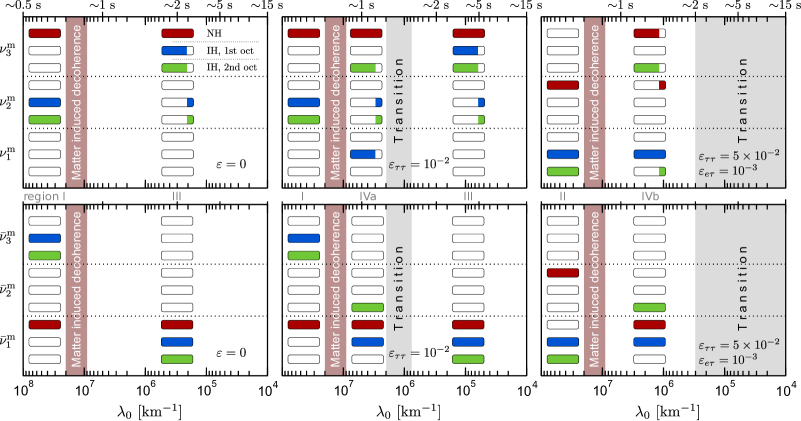
Figure 6.15: Relationship between $\nu_{e}$ (top panels) and $\bar{\nu}_{e}$ (bottom panels) and the matter eigenstates at the SN surface as function of time for different neutrino mass and mixing schemes and for given values of $\varepsilon_{\tau\tau}=0$ (left), $3\times 10^{-2}$ (middle), and $5\times 10^{-2}$ (right).

Throughout the analysis we have limited ourselves to the case of NSI with $d$ quarks. Nevertheless most of the results here presented can be generalized to the case of $u$ quarks and $e$. In the first case the only effect is to shift the position of the $I$-resonance, since the resonance condition is modified to $Y_{e}^{I}=\varepsilon_{\tau\tau}/(1-\varepsilon_{\tau\tau})$  [21]. In the case of $e$ the $I$-resonance is absent. But nevertheless its contribution to increase the value of $Y^{\rm eff}_{\rm\tau,nsi}$ would also make the neutrino propagation highly sensitive to the $\theta_{23}$ octant and to its own sign, exactly as in the case of $d$ quark.

Last but not least we briefly comment on the possibility to observe the different regimes analyzed. This possibility will be hampered by several uncertainties inherent in SN neutrinos. One is the lack of knowledge on the exact matter profile traversed by the outgoing neutrinos. In our study we assumed a simple power law given in Eq. (6.34). This density profile will be significantly distorted by the passage of the shock wave responsible for ejecting the whole SN envelope [70, 180, 181]. One of the main effect will be to destroy the adiabaticity of the $H$-resonance, which was assumed in the study. This effect, though, is not always present but depends on the neutrino properties. Therefore, far from being a problem, the time and energy dependence modulation introduced in the spectra could further help disentangle between the different scenarios here considered [71, 66, 21].

Another important source of uncertainties is our ignorance of the exact initial fluxes $f^{\rm R}_{\nu_{\alpha}}(E)$. Although the initial fluxes during the first stage of the explosion, the neutronization burst, are rather model independent [202], the expected number of events is very low. Most of the signal is generated later, during the accretion and cooling phases. The spectral features observed in the numerical simulations depends strongly on the properties of the SN. It is therefore necessary to set up strategies combining different observables to be able to pin down the underlying neutrino properties independently of the initial fluxes. These include among others to analyze the spectral modulations expected if neutrinos cross the Earth before being detected [203, 204, 205, 206], or benefit from the time dependence of the matter profiles $\lambda(r)$ and $Y_{e}(r)$ themselves [21].

6.4 Summary

We have reexamined the effect of NSI on the neutrino propagation through the SN envelope within a three-neutrino framework, first in the absence and later in the presence of a neutrino background. We have found that the small values of the electron fraction, typical of the more deleptonized inner layers, allow for internal NSI-induced resonant conversions, in addition to the standard MSW-H and MSW-L resonances of the outer envelope. These new flavor conversions take place for a relatively large range of NSI parameters, namely $|\varepsilon_{\alpha\alpha}|$ between $10^{-2}-10^{-1}$, and $|\varepsilon_{e\tau}|\gtrsim{\rm few}\times 10^{-5}$, currently allowed by experiment. For this range of strengths, in particular $\varepsilon_{\tau\tau}$, NSI can significantly affect the adiabaticity of the $H$-resonance. We have also obtained that when including neutrino self-interaction to the system and considering $|\varepsilon_{\tau\tau}|\gtrsim$ few$\times 10^{-4}$ the neutrino propagation becomes for some time sensitive to the $\theta_{23}$ octant and the sign of $\varepsilon_{\tau\tau}$. Furthermore, the coexistence of collective effects and the $I$-resonance may lead to an exchange of the neutrino fluxes entering the bipolar regime. The main consequences being a bipolar conversion happening for normal mass hierarchy and an inverted spectral split.

Chapter 7 Conclusions

Neutrino physics has reached a point where one can start talking about precision physics. In the last ten years the situation has changed from having no experimental evidence of massive neutrinos to measuring the oscillation parameters within errors of 5% to 10%. The conditions are, therefore, ideal for the study of neutrino non-standard properties while we improve the precision in the measurement of their oscillation parameters. These two research lines, together with the determination of the Dirac or Majorana nature of neutrinos, are nowadays centering the effort of the neutrino physicists community. The thesis here presented has followed this philosophy. We have analyzed various aspects of neutrino phenomenology in two different scenarios: accelerator and reactor terrestrial experiments, and neutrinos in a supernova (SN) environment.

In this way, we have started with a series of introductory chapters, where we have reviewed, in a general form, the physics of SN explosions, neutrino oscillations and the effect of non-standard interaction (NSI). With these important concepts already clarified, we have discussed whether OPERA could help in constraining neutrino NSI, improving the results obtained from MINOS and Double Chooz. The motivation for this study is twofold. Firstly, OPERA will measure for the first time the oscillation $\nu_{\mu}\to\nu_{\tau}$, detecting directly the $\nu_{\tau}$; secondly, the distance-energy ($L/E$) relation is very different for MINOS and OPERA. Both conditions could help in distinguishing NSI from standard oscillations. The inclusion of Double Chooz into the analysis limits $\theta_{13}$ in an independent way, since it is not sensitive to NSI because of the short distance involved and the low energy of its neutrinos. In our study we have obtained that the main improvement coming from OPERA is due to the different $L/E$ relation with respect to MINOS. However, the limits we got from their combination do not increase the precision obtained with atmospheric neutrino experiments. Furthermore, the expected $\nu_{\tau}$ signal in OPERA is too low to be of statistical significance, helping only for large values of $\theta_{13}$.

Regarding the main neutrino scenario discussed in this thesis, i.e. core collapse SN, we have essentially focused on two effects. On the one hand, we have analyzed neutrino self-interaction in the SN envelope, recently confirmed to be of special importance in their evolution. This piece of the system had been underestimated for a long time, and only very recently its relevance has been recognized, drastically changing SN neutrino’s evolution paradigm. Before this discovery, their evolution was basically determined by the adiabaticities of the MSW $H$ and $L$-resonances. In contrast, it has been shown that neutrino collective conversion effects can occur in the most inner layers of the star, given the appropriate astrophysical (matter and neutrino densities, hierarchy of fluxes$\dots$) and neutrino (inverted mass hierarchy) conditions. The nature of these transformations is very different from that of the standard resonances.

In this thesis we have reviewed the collective transformation phenomenon. We have payed special attention to the most relevant effects, mainly the inversion of the neutrino fluxes entering the MSW resonances, and the spectral split. Keeping this in mind, we have studied, in a two flavor scenario, the consequences that could result from the multi-angular nature of the system, being neutrinos emitted from a spherical surface, the neutrino sphere. This condition can induce kinematical decoherence, since different angular modes feel different refraction index in the medium. We have identified two possible sources of decoherence, one related to the self-interaction term, and another to the interaction with matter, which will have different magnitude depending on the emission angle. From our study we conclude that the first one does not involve any risk, given the characteristics obtained in the simulations of this kind of explosions. The second source, in contrast, translates into a time dependence of the expected signal. At the initial moments of the explosion, when the matter density near the neutrino sphere is much larger than the neutrino one, a suppression of the collective phenomenon is obtained. As time goes on, the matter density is reduced becoming comparable to the neutrino one. We then obtain a transition region marked by the decoherence. Nevertheless, the matter density will quickly become lower than that of neutrinos, recovering the collective effects. After having clarified the decoherence topic, we have studied the existence of possible characteristic three-flavor effects. In summary, we have obtained that in the absence of second order corrections to the potentials affecting $\nu_{\mu}$ and $\nu_{\tau}$, the system can be always reduced to the two flavor case. However, if we take into account the radiative corrections, the $\nu_{e}$ and $\bar{\nu}_{e}$ survival probabilities can be modified, and depend on the $\theta_{23}$ octant. This effect however, requires a large matter density, which in turn would suppress the collective effect.

The second important point we have discussed in the SN scenario is the effect that the inclusion of the possible NSI would induce in the neutrino propagation. This effect occur in the same region where collective neutrino transformation phenomena take place. Therefore, we have first clarified the genuine NSI effects by initially neglecting any self-interaction effect. The most important consequence we have obtained in our study is the appearance of a new resonance ($I$) in the internal regions of the SN. It is related to the low values of the electron fraction in the most deleptonized layers of the star, near the neutrino sphere. Furthermore, we obtain a modification in the $H$ and $L$-resonance conditions, basically affecting their positions. The interplay of NSI and neutrino self-interactions has very interesting consequences for the propagation of SN neutrinos. First, the time dependence of the collective effects is modified in the presence of NSI. For some time, the evolution of neutrinos becomes sensitive to the octant of $\theta_{23}$ and the sign of $\varepsilon_{\tau\tau}$, provided that $|\varepsilon_{\tau\tau}|\gtrsim 10^{-4}$. This is an analogous effect to that obtained as a consequence of the radiative corrections to the potentials. The difference here is that the presence of NSI lowers the density required to induce the effect, and the tension with the suppression of the collective effects is therefore relaxed. On the other hand, if $|\varepsilon_{\tau\tau}|\gtrsim 10^{-2}$ the $I$-resonance comes into play, which in the case of being adiabatic will transform the neutrino fluxes entering the bipolar region. As a consequence, we will obtain bipolar conversion for normal mass hierarchy case and an inverted spectral split.

Conclusions

La física de neutrins ha arribat a un punt en què pot començar a parlar-se de física de precisió. En els darrers deu anys s’ha passat de no tindre cap evidència experimental de la massa dels neutrins a la determinació dels paràmetres d’oscil$\cdot$lació amb errors entre el 5% i el 10%. Es donen, doncs, les condicions per a buscar possibles propietats no estàndard dels neutrins alhora que s’incrementa la precisió en la mesura dels seus paràmetres. Aquestes dues línies d’investigació, junt a la determinació de la naturalesa de Dirac o Majorana dels neutrins, centren actualment els esforços de la comunitat de físics de neutrins. La tesi ací presentada ha seguit aquesta filosofia. Hem fet una anàlisi de diversos aspectes de fenomenologia de neutrins en dos escenaris diferents: per un costat experiments terrestres d’accelerador i reactor i per un altre neutrins emesos per una supernova (SN).

Així doncs, hem començat amb una sèrie de capítols introductoris on hem revisat de forma general la física de les explosions de SN, d’oscil$\cdot$lació de neutrins i les seues possibles interaccions no estàndard (NSI). Amb aquests conceptes clarificats, hem discutit la possibilitat de millorar els límits sobre les NSI obtinguts als experiments MINOS i Double Chooz amb la inclusió d’OPERA. La motivació d’aquesta anàlisi és doble. En primer lloc, OPERA és el primer experiment capaç de mesurar l’oscil$\cdot$lació $\nu_{\mu}\to\nu_{\tau}$ detectant directament els $\nu_{\tau}$; en segon lloc, la relació distància-energia ($L/E$) és molt diferent entre MINOS i OPERA. Totes dues condicions podrien ajudar a distingir entre oscil$\cdot$lacions estàndard i NSI. La inclusió de Double Chooz en l’anàlisi permet limitar de forma independent $\theta_{13}$, ja que no és sensible a les NSI degut a la curta distància involucrada i la baixa energia dels neutrins. Al nostre estudi hem trobat que la principal millora que OPERA aporta ve de la seua diferència en $L/E$ respecte a MINOS. Tot i això, els límits que s’obtenen no augmenten la precisió aconseguida en experiments amb neutrins atmosfèrics. D’altra banda, el senyal de $\nu_{\tau}$ esperat en OPERA és massa baix per a ser estadísticament significatiu, ajudant només per a valors grans de $\theta_{13}$.

Respecte al principal escenari de neutrins discutit en aquesta tesi, les explosions de SN per col$\cdot$lapse gravitatori del nucli, ens hem centrat essencialment en dos efectes. D’un costat, hem analitzat l’autointeracció dels propis neutrins en la seua propagació a través de la SN, recentment constatat com d’especial importància en la seua evolució. Aquesta peça del sistema havia sigut menyspreada durant molt de temps, i només als darrers anys s’ha reconegut la seua rellevància, canviant dràsticament el paradigma d’evolució de neutrins de SN. Abans d’aquest descobriment, la seua evolució venia determinada bàsicament per l’adiabaticitat de les ressonàncies MSW: $H$ i $L$. Per contra, s’ha vist que en la regió interna de l’estel, donades les condicions apropiades tant astrofísiques (densitat de matèria i de neutrins, jerarquia de fluxos per als diferents sabors de neutrins$\dots$) com dels propis neutrins (jerarquia inversa de massa), poden ocórrer efectes col$\cdot$lectius de conversió de sabor en neutrins i antineutrins, de naturalesa molt diferent a la de les ressonàncies estàndard.

En aquesta tesi hem fet, doncs, una revisió del fenomen parant especial atenció als efectes més destacats, que principalment són la inversió del flux de neutrins que entren en les ressonàncies MSW i el “trencament de l’espectre” (spectral split). Partint d’aquesta base, hem estudiat, en un escenari de dos sabors, les conseqüències que la naturalesa multiangular del sistema pot tindre en la seua evolució, per ser els neutrins emesos des d’una superfície esfèrica, la neutrinosfera. Aquesta condició pot donar lloc a una decoherència cinemàtica en el sistema, ja que els diferents modes angulars senten diferent índex de refracció amb el medi. Hem identificat dues possibles fonts de decoherència, una deguda al terme d’autointeracció dels neutrins, i altra a la interacció amb la matèria, que tindrà diferent intensitat segons l’angle d’emissió. Del nostre estudi concloem que la primera no suposa un perill per a l’estudi de neutrins de SN, donades les característiques que típicament s’obtenen en les simulacions d’aquest tipus d’explosions. La segona font, per contra, comporta una dependència temporal del senyal esperat. En els instants inicials de l’explosió, quan la densitat de matèria prop de la neutrinosfera és molt gran comparada amb la de neutrins, s’obté una supressió del fenomen col$\cdot$lectiu. Conforme passa el temps la densitat de matèria disminueix fent-se comparable a la de neutrins. S’obté, aleshores, una regió de transició marcada per la decoherència i per tant pèrdua de la informació de l’espectre incial dels neutrins. No obstant, la densitat de matèria ràpidament es farà inferior a la de neutrins, recuperant l’efecte col$\cdot$lectiu. Una vegada aclarit el tema de la decohèrencia, hem estudiat l’existència de possibles efectes característics de tres sabors. En resum, hem obtingut que en absència de correccions de segon ordre als potencials que afecten els $\nu_{\mu}$ i $\nu_{\tau}$, el sistema pot ser reduït sempre al cas de dos sabors. No obstant, si tenim en compte les correccions radiatives als potencials, les probabilitats de supervivència dels $\nu_{e}$ i $\bar{\nu}_{e}$ es poden veure dràsticament modificades, depenent sensiblement de l’octant de $\theta_{23}$. Aquest efecte però, precisa d’una alta densitat de matèria, i possiblement estiga amagat sota la supressió del fenomen col$\cdot$lectiu que això comporta.

El segon punt important que hem tractat dins d’un escenari de SN és l’efecte que la inclusió de possibles NSI tindria en la propagació dels neutrins. Aquestes afecten en la mateixa regió interna de la SN on tenen lloc els fenòmens de transformació col$\cdot$lectiva de neutrins. Per tant, hem volgut clarificar primer els efectes genuïns de les NSI, analitzant inicialment el sistema en absència d’autointeracció dels neutrins. La conseqüència més important d’aquest estudi és l’aparició d’una nova ressonància ($I$) en les regions internes de la SN, relacionada amb valors xicotets de la fracció electrònica en la zona més deleptonizada de l’estel, prop de la neutrinosfera. A més a més, s’obté una modificació en les condicions de les ressonàncies $H$ i $L$, bàsicament afectant a la seua posició. L’estudi conjunt de les NSI i l’autointeracció dels neutrins té conseqüències molt interessants per a la propagació dels neutrins de SN. En primer lloc, la dependència temporal dels fenòmens col$\cdot$lectius es veu modificada per la presència de les NSI. Durant un cert temps la propagació dels neutrins es torna sensible a l’octant de $\theta_{23}$ i al signe de $\varepsilon_{\tau\tau}$, sempre i quan $|\varepsilon_{\tau\tau}|\gtrsim 10^{-4}$. Aquest efecte és anàleg al que obteníem degut a les correccions radiatives, amb la diferència que la presència de NSI disminueix la densitat requerida per a induir l’efecte. Es relaxa així la tensió amb la supressió del fenomen col$\cdot$lectiu deguda a l’alta densitat de matèria. D’un altre costat, si $|\varepsilon_{\tau\tau}|\gtrsim 10^{-2}$ la ressonància $I$ entrarà en joc, la qual, en cas de ser adiabàtica, transformarà els fluxos de neutrins que entren a la regió bipolar. Com a conseqüència obtindrem conversió bipolar per a jerarquia normal de masses i un trencament de l’espectre invers.

Appendix A

Equations of motion

A.1 Temporal evolution

A homogeneous ensemble of unmixed neutrinos is represented by the occupation numbers $f_{\bf p}=\langle a^{\dagger}_{\bf p}a_{\bf p}\rangle$ for each momentum mode ${\bf p}$, where $a^{\dagger}_{\bf p}$ and $a_{\bf p}$ are the relevant creation and annihilation operators and $\langle\ldots\rangle$ is the expectation value. A corresponding expression can be defined for the antineutrinos, ${\bar{f}}_{\bf p}=\langle{\bar{a}}^{\dagger}_{\bf p}{\bar{a}}_{\bf p}\rangle$, where overbarred quantities always refer to antiparticles. In a multiflavor system of mixed neutrinos, the occupation numbers are generalised to density matrices in flavor space [207, 176, 208]

$$(\varrho_{\bf p})_{ij}=\langle a^{\dagger}_{i}a_{j}\rangle_{\bf p}\hbox{\quad and\quad}(\bar{\varrho}_{\bf p})_{ij}=\langle\bar{a}^{\dagger}_{j}\,\bar{a}_{i}\rangle_{\bf p}\,.$$ (A.1)

The reversed order of the flavor indices $i$ and $j$ in the right-hand side for antineutrinos assures that $\varrho_{\bf p}$ and $\bar{\varrho}_{\bf p}$ transform identically under a flavor transformation.

Flavor oscillations of an ensemble of neutrinos and antineutrinos are described by [207, 176, 208]

$${\rm i}\partial_{t}\varrho_{\bf p}=[{\sf H}_{\bf p},\varrho_{\bf p}]\hbox{\quad and\quad}{\rm i}\partial_{t}\bar{\varrho}_{\bf p}=[\bar{\sf H}_{\bf p},\bar{\varrho}_{\bf p}]\,,$$ (A.2)

where $[{\cdot},{\cdot}]$ is a commutator. The “Hamiltonian” for each mode is

$${\sf H}_{\bf p}=\Omega_{\bf p}+\lambda{\sf L}+\sqrt{2}\,G_{\rm F}\int\!\frac{{\rm d}^{3}{\bf q}}{(2\pi)^{3}}\left(\varrho_{\bf q}-\bar{\varrho}_{\bf q}\right)(1-{\bf v}_{\bf q}\cdot{\bf v}_{\bf p})\,,$$ (A.3)

where $G_{\rm F}$ is the Fermi constant. The matrix of vacuum oscillation frequencies for relativistic neutrinos is in the mass basis $\Omega_{\bf p}={\rm diag}(m_{1}^{2},m_{2}^{2},m_{3}^{2})/2p$ with $p=|{\bf p}|$. The matter effect is represented by $\lambda=\sqrt{2}\,G_{\rm F}(n_{e^{-}}-n_{e^{+}})$ and ${\sf L}={\rm diag}(1,0,0)$, given here in the weak interaction basis. We ignore the possible presence of other charged-lepton flavors. The Hamiltonian for antineutrinos $\bar{\sf H}_{\bf p}$ is the same with $\Omega_{\bf p}\to-\Omega_{\bf p}$, i.e., in vacuum antineutrinos oscillate “the other way round.”

The factor $(1-{\bf v}_{\bf q}\cdot{\bf v}_{\bf p})=(1-\cos\theta_{\bf pq})$ represents the current-current nature of the weak interaction where ${\bf v}_{\bf p}={\bf p}/p$ is the velocity. The angular term averages to zero if the gas is isotropic. We ignore a possible net flux of charged leptons lest the ordinary matter effect also involves an angular factor.

If the system is axially symmetric relative to some direction, the angular factor simplifies after an azimuthal integration to [160, 164]

$$(1-{\bf v}_{\bf q}\cdot{\bf v}_{\bf p})\to(1-{v}_{\bf q}{v}_{\bf p})\,,$$ (A.4)

where the velocities are along the symmetry axis.

A.2 Spatial evolution in spherical symmetry

Instead of a homogeneous system that evolves in time we consider a stationary system that evolves in space. The occupation numbers become Wigner functions, which depend both on spatial coordinates and on momenta, but there is no conceptual problem as long as we consider spatial variations that are slow on the scale of the inverse neutrino momenta.

Since multi-angle effects are at the focus of our problem, we cannot reduce the equations to plane waves moving in the same direction. Motivated by the SN application, however, we can take advantage of global spherical symmetry, implying that the ensemble is represented by matrices that depend on a radial coordinate $r$, the zenith angle relative to the radial direction, and the energy $E$ which in the relativistic limit is identical with $p=|{\bf p}|$.

We ignore gravitational deflection near the SN core and assume that neutrinos move on straight lines after being launched at a radius $R$ that we call the neutrino sphere. Consider a neutrino that was launched at an angle $\vartheta_{R}$ relative to the radial direction. Its radial velocity is

$$v_{R}=\cos\vartheta_{R}\,.$$ (A.5)

At $r>R$ the trajectory’s angle relative to the radial direction is implied by simple geometry to be [160] (see e.g. their Fig. 1)

$$R\sin\vartheta_{R}=r\sin\vartheta_{r}\,.$$ (A.6)

Therefore, the radial velocity at $r$ is

$$v_{u,r}=\cos\vartheta_{r}=\sqrt{1-\frac{R^{2}}{r^{2}}\,u}$$ (A.7)

where we have introduced

$$u=1-v^{2}_{R}=\sin^{2}\vartheta_{R}\,.$$ (A.8)

It is convenient to label the angular modes with $u$. The physical zenith angles change with distance so that the equations would be more complicated.

The density matrices $\varrho_{p,u,r}$ are not especially useful to describe a spherically symmetric system because they vary with $r$ even in the absence of oscillations. (Note that we often write the dependence of a quantity on a variable as an subscript.) A quantity that is conserved in the absence of oscillations is the total flux matrix

$${\sf J}_{r}=\frac{r^{2}}{R^{2}}\int\frac{{\rm d}^{3}{\bf p}}{(2\pi)^{3}}\,\varrho_{{\bf p},r}\,v_{{\bf p},r}\,.$$ (A.9)

To express the integral in co-moving variables we observe that ${\rm d}^{3}{\bf p}$ in spherical coordinates is $p^{2}{\rm d}p\,{\rm d}\varphi\,{\rm d}\cos\vartheta_{r}$ and that Eq. (A.7) implies

$$\left|\frac{{\rm d}\cos\vartheta_{r}}{{\rm d}u}\right|=\frac{1}{2v_{u,r}}\,\frac{R^{2}}{r^{2}}\,.$$ (A.10)

Therefore, we finally define the differential flux matrices

$${\sf J}_{p,u,r}=\frac{p^{2}\varrho_{p,u,r}}{2\,(2\pi)^{2}}\,,$$ (A.11)

where we have used $\int{\rm d}\varphi=2\pi$ for axial symmetry. The normalization is

$${\sf J}_{r}=\int_{0}^{1}{\rm d}u\int_{0}^{\infty}{\rm d}p\;{\sf J}_{p,u,r}\,.$$ (A.12)

In the absence of oscillations the total and differential fluxes are conserved, $\partial_{r}{\sf J}_{r}=0$ and $\partial_{r}{\sf J}_{p,u,r}=0$.

To include oscillations, we note that the radial velocity along a neutrino trajectory is $v_{u,r}={\rm d}r_{u}/{\rm d}t=\cos\vartheta_{u,r}$. Therefore, if we wish to express the temporal evolution of the neutrino density matrix along its trajectory in terms of an evolution expressed in terms of the radial coordinate $r$, we substitute $\partial_{t}\to v_{u,r}\partial_{r}$ in Eq. (A.2) so that

$${\rm i}\partial_{r}{\sf J}_{p,u,r}=\frac{[{\sf H}_{p,u,r},{\sf J}_{p,u,r}]}{v_{u,r}}\,,$$ (A.13)

and analogous for antineutrinos. In other words, we project the evolution along a given trajectory to an evolution along the radial direction. For vacuum oscillations this has the effect of “compressing” the oscillation pattern for non-radial modes, i.e., even for monochromatic neutrinos, the effective vacuum oscillation frequency depends on both $r$ and $u$.

The vacuum-oscillation and ordinary-matter contributions to ${\sf H}_{p,u,r}$ were given in Eq. (A.3), whereas the self-term must be made explicit. To this end we introduce the matrix of number densities

$${\sf N}_{p,u,r}=v_{u,r}^{-1}\,{\sf J}_{p,u,r}$$ (A.14)

and its integral as

$${\sf N}_{r}=\int_{0}^{1}{\rm d}u\int_{0}^{\infty}{\rm d}p\;{\sf N}_{p,u,r}=\int_{0}^{\infty}{\rm d}u\int_{0}^{\infty}{\rm d}p\;\frac{{\sf J}_{p,u,r}}{v_{u,r}}\,.$$ (A.15)

Collecting all terms and taking advantage of Eq. (A.4) for axial symmetry, we find

$${\rm i}\partial_{r}{\sf J}_{p,u,r} = +\bigl{[}\Omega_{p},{\sf N}_{p,u,r}\bigr{]}+\lambda_{r}\bigl{[}{\sf L},{\sf N}_{p,u,r}\bigr{]}$$

$$+\sqrt{2}G_{\rm F}\,\frac{R^{2}}{r^{2}}\,\Bigl{(}\bigl{[}{\sf N}_{r}-\bar{\sf N}_{r},{\sf N}_{p,u,r}\bigr{]}-\bigl{[}{\sf J}_{r}-\bar{\sf J}_{r},{\sf J}_{p,u,r}\bigr{]}\Bigr{)}\,,$$

$${\rm i}\partial_{r}\bar{\sf J}_{p,u,r} = -\bigl{[}\Omega_{p},\bar{\sf N}_{p,u,r}\bigr{]}+\lambda_{r}\bigl{[}{\sf L},\bar{\sf N}_{p,u,r}\bigr{]}$$ (A.16)

$$+\sqrt{2}G_{\rm F}\,\frac{R^{2}}{r^{2}}\,\Bigl{(}\bigl{[}{\sf N}_{r}-\bar{\sf N}_{r},\bar{\sf N}_{p,u,r}\bigr{]}-\bigl{[}{\sf J}_{r}-\bar{\sf J}_{r},\bar{\sf J}_{p,u,r}\bigr{]}\Bigr{)}\,,$$

where the electron density’s radial variation is included in $\lambda_{r}$.

A.3 Angular emission characteristics

In a numerical simulation we need to specify the fluxes at the neutrino sphere $r=R$. For our usual multi-angle simulations we assume that the neutrino radiation field is “half isotropic” directly above the neutrino sphere, i.e., that all outward-moving angular modes are equally occupied as behooves a thermal radiation field. Therefore, the occupation numbers are distributed as ${\rm d}n/{\rm d}\cos\vartheta_{R}={\rm const.}$, implying that the radial fluxes are distributed as ${\rm d}j/{\rm d}\cos\vartheta_{R}=v_{R}{\rm d}n/{\rm d}\cos\vartheta_{R}\propto\cos\vartheta_{R}$ because $v_{R}=\cos\vartheta_{R}$. Expressed in the angular variable $u$ this implies ${\rm d}j/{\rm d}u={\rm const.}$ because of Eq. (A.10). In other words, a blackbody radiation field at the neutrino sphere implies that

$${\sf J}_{u}={\rm const.}$$ (A.17)

in the interval $0\leq u\leq 1$.

To avoid multi-angle effects one may sometimes wish to use a single angular bin. To represent a uniform ${\sf J}_{u}$ distribution, the natural choice is $u=1/2$, corresponding to a launch angle $\vartheta_{R}=45^{\circ}$. Our numerical single-angle examples always correspond to this choice in an otherwise unchanged numerical code.

In this case the radial velocity of all neutrinos as a function of radius is

$$v_{r}=\sqrt{1-\frac{R^{2}}{2r^{2}}}\,.$$ (A.18)

For a monochromatic spectrum, the remaining flavor matrices are simply the total ${\sf J}_{r}$ (corresponding to the single $u=1/2$) and ${\sf N}_{r}={\sf J}_{r}/v_{r}$. Ignoring the trivial ordinary matter term, the equations of motion are

$${\rm i}\partial_{r}{\sf J}_{r}=\frac{\bigl{[}\Omega,{\sf J}_{r}\bigr{]}}{v_{r}}+\sqrt{2}G_{\rm F}\,\frac{R^{2}}{r^{2}}\,\left(\frac{1}{v_{r}^{2}}-1\right)\bigl{[}{\sf J}_{r}-\bar{\sf J}_{r},{\sf J}_{r}\bigr{]}$$ (A.19)

and analogous for the antineutrinos. The coefficient of the neutrino-neutrino term is explicitly

$$\sqrt{2}G_{\rm F}\,\frac{R^{4}}{r^{4}}\,\frac{1}{2-R^{2}/r^{2}}\,.$$ (A.20)

At the neutrino sphere this expression becomes equal to $\sqrt{2}G_{\rm F}$, whereas at large distances it is $(\sqrt{2}G_{\rm F}/2)\,R^{4}/r^{4}$. As observed in the previous literature, the neutrino-neutrino term dies out at large distances as $r^{-4}$.

One can define a “single-angle case” somewhat differently. Assuming all angular modes evolve coherently, we can integrate the equations of motion over $\int_{0}^{1}{\rm d}u$ and study the evolution of the quantities $J_{p,r}=\int_{0}^{1}{\rm d}uJ_{p,u,r}$. To write the equations in a compact form we introduce the notation

$$\frac{1}{v_{r}^{*}}\equiv\frac{1}{{\sf J}_{r}}\int_{0}^{\infty}\!{\rm d}p\int_{0}^{1}{\rm d}u\;\frac{{\sf J}_{p,u,r}}{v_{u,r}}\,.$$ (A.21)

The full equation of motion Eq. (A.2) for neutrinos becomes

$${\rm i}\partial_{r}{\sf J}_{p,r} = \frac{\bigl{[}\Omega_{p},{\sf J}_{p,r}\bigr{]}}{v_{r}^{*}}+\lambda_{r}\,\frac{\bigl{[}{\sf L},{\sf J}_{p,r}\bigr{]}}{v_{r}^{*}}$$ (A.22)

$${}+\sqrt{2}G_{\rm F}\,\frac{R^{2}}{r^{2}}\,\left(\frac{1}{(v_{r}^{*})^{2}}-1\right)\bigl{[}{\sf J}_{r}-\bar{\sf J}_{r},{\sf J}_{p,r}\bigr{]}$$

and analogous for antineutrinos with $\Omega_{p}\to-\Omega_{p}$.

At large distances we have $1/v_{r}^{*}=1+\frac{1}{2}(R/r)^{2}\langle u\rangle$ where $\langle u\rangle$ is the average of $u$ at emission. For the vacuum and matter terms, we only need the leading terms so that we recover the familiar plane-wave form of the equations of motion. The coefficient of the neutrino-neutrino term, on the other hand, becomes

$$\sqrt{2}G_{\rm F}\,\frac{R^{4}}{r^{4}}\,\langle u\rangle\,.$$ (A.23)

Both for half-isotropic emission and for our single-angle case we have $\langle u\rangle=\frac{1}{2}$, in agreement with Eq. (A.20).

Agraïments/Acknowledgements

En primer lloc vull agrair als meus directors de tesi, Jose W. Furtado Valle i Ricard Tomàs Bayo, perquè ells han fet possible la realització d’aquesta tesi doctoral, cadascun amb la seua responsabilitat.

I would also like to thank everyone whom I have had the opportunity to work with: Alessandro Mirizzi, Georg G. Raffelt, Günter Sigl, Pasquale D. Serpico, Patrick Huber and Sergio Pastor. It has been a pleasure to be your coauthor. I have learnt a lot from all of you.

Dejando de lado la física, pero sin salir del IFIC, quiero agradecer a toda la gente que ha hecho que estos cuatro años y pico de doctorado me hayan dejado tan buen recuerdo. Muchas gracias a toda la gente que está, o ha pasado por el grupo AHEP: Diego Aristizábal, Tegua, Albert, Mariam, Urbano, Avelino, Martin, Diego Restrepo, Massimiliano, Timur, Federica, Satoru, Antonio, Stefano, Werner, Celio, Omar, Juan, Thomas, Sofiane, Kiko, Laslo$\ldots$ Muchas gracias también a todos los amigotes del IFIC: Martín, Diego Milanés, Paola, Alberto, Fabio, Paula, Natxo, la gente del futbito$\ldots$ y a los de la universidad: Iván, Enrique, Jacobo, Ana, Víctor$\ldots$

Doble agraïment mereix Ricard, perquè no només m’has guiat durant tot el meu doctorat sinó que a més has fet que el món de la física prengués un altre sentit, sempre amb eixa visió tan particular$\ldots$ tu m’entens.

Por supuesto quiero agradecer a mi familia, que siempre está ahí y me ha sufrido desde el principio de los días, porque aunque hace tiempo que se fue “Sor Oxidación de los Clavos de la Cruz”, tengo mis momentos. Muchísimas gracias a mis padres, Julián y María, a mis hermanos Julen y Guille, a mis cuñadas Jean y Ana, a mi futuro sobrinito Pau, a Cecilia y por supuesto a Julia (la chica guapa del IFIC), donde empieza mi nueva familia.

Por último, quiero agradecer a mis amigos de la “Pandilla led Infiern”. Aunque nunca os hayáis creído el rollo de los neutrinos y mucho menos que sirvan para nada, os merecéis un hueco especial en esta tesis. Nos vemos en el TeOdio: Aida y Pepetoni, Ferran y Alba, Carlos, Germán, Goyo y María, Feli y Alex, Ariana e Iván.

Bibliography

- [1] Y. Fukuda et al. [Super-Kamiokande Collaboration], “Evidence for oscillation of atmospheric neutrinos,” Phys. Rev. Lett. 81 (1998) 1562 [arXiv:hep-ex/9807003].
- [2] K. Eguchi et al. [KamLAND Collaboration], “First results from KamLAND: Evidence for reactor anti-neutrino disappearance,” Phys. Rev. Lett. 90 (2003) 021802 [arXiv:hep-ex/0212021].
- [3] M. H. Ahn et al. [K2K Collaboration], “Indications of Neutrino Oscillation in a 250 km Long-baseline Experiment,” Phys. Rev. Lett. 90 (2003) 041801 [arXiv:hep-ex/0212007].
- [4] D. G. Michael et al. [MINOS Collaboration], “Observation of muon neutrino disappearance with the MINOS detectors and the NuMI neutrino beam,” Phys. Rev. Lett. 97 (2006) 191801 [arXiv:hep-ex/0607088].
- [5] A. B. McDonald, “Solar neutrino measurements,” New J. Phys. 6 (2004) 121 [arXiv:astro-ph/0406253].
- [6] T. Schwetz, M. Tortola and J. W. F. Valle, “Three-flavour neutrino oscillation update,” New J. Phys. 10 (2008) 113011 [arXiv:0808.2016 [hep-ph]].
- [7] J. Schechter and J. W. F. Valle, “Majorana Neutrinos And Magnetic Fields,” Phys. Rev. D 24 (1981) 1883 [Erratum-ibid. D 25 (1982) 283].
- [8] E. K. Akhmedov, “Resonant amplification of neutrino spin rotation in matter and the solar-neutrino problem,” Phys. Lett. B 213 (1988) 64.
- [9] L. Wolfenstein, “Neutrino oscillations in matter,” Phys. Rev. D 17 (1978) 2369.
- [10] A. Esteban-Pretel, J. W. F. Valle and P. Huber, “Can OPERA help in constraining neutrino non-standard interactions?,” Phys. Lett. B 668 (2008) 197 [arXiv:0803.1790 [hep-ph]].
- [11] S. Pastor and G. Raffelt, “Flavor oscillations in the supernova hot bubble region: Nonlinear effects of neutrino background,” Phys. Rev. Lett. 89 (2002) 191101 [arXiv:astro-ph/0207281].
- [12] R. F. Sawyer, “Speed-up of neutrino transformations in a supernova environment,” Phys. Rev. D 72 (2005) 045003 [arXiv:hep-ph/0503013].
- [13] G. M. Fuller and Y. Z. Qian, “Simultaneous flavor transformation of neutrinos and antineutrinos with dominant potentials from neutrino-neutrino forward scattering,” Phys. Rev. D 73 (2006) 023004 [arXiv:astro-ph/0505240].
- [14] S. Hannestad, G. G. Raffelt, G. Sigl and Y. Y. Y. Wong, “Self-induced conversion in dense neutrino gases: Pendulum in flavour space,” Phys. Rev. D 74 (2006) 105010 [Erratum-ibid. D 76 (2007) 029901] [arXiv:astro-ph/0608695].
- [15] G. G. Raffelt and A. Y. Smirnov, “Self-induced spectral splits in supernova neutrino fluxes,” Phys. Rev. D 76 (2007) 081301 [Erratum-ibid. D 77 (2008) 029903] [arXiv:0705.1830 [hep-ph]].
- [16] G. L. Fogli, E. Lisi, A. Marrone and A. Mirizzi, “Collective neutrino flavor transitions in supernovae and the role of trajectory averaging,” JCAP 0712 (2007) 010 [arXiv:0707.1998 [hep-ph]].
- [17] A. Esteban-Pretel, S. Pastor, R. Tomàs, G. G. Raffelt and G. Sigl, “Decoherence in supernova neutrino transformations suppressed by deleptonization,” Phys. Rev. D 76 (2007) 125018 [arXiv:0706.2498 [astro-ph]].
- [18] A. Esteban-Pretel, S. Pastor, R. Tomàs, G. G. Raffelt and G. Sigl, “Mu-tau neutrino refraction and collective three-flavor transformations in supernovae,” Phys. Rev. D 77 (2008) 065024 [arXiv:0712.1137 [astro-ph]].
- [19] B. Dasgupta, A. Dighe, A. Mirizzi and G. G. Raffelt, “Spectral split in prompt supernova neutrino burst: Analytic three-flavor treatment,” Phys. Rev. D 77 (2008) 113007 [arXiv:0801.1660 [hep-ph]].
- [20] A. Esteban-Pretel, A. Mirizzi, S. Pastor, R. Tomàs, G. G. Raffelt, P. D. Serpico and G. Sigl, “Role of dense matter in collective supernova neutrino transformations,” Phys. Rev. D 78 (2008) 085012 [arXiv:0807.0659 [astro-ph]].
- [21] A. Esteban-Pretel, R. Tomàs and J. W. F. Valle, “Probing non-standard neutrino interactions with supernova neutrinos,” Phys. Rev. D 76 (2007) 053001 [arXiv:0704.0032 [hep-ph]].
- [22] A. Esteban-Pretel, R. Tomas and J. W. F. Valle, “Interplay between collective effects and non-standard neutrino interactions of supernova neutrinos,” arXiv:0909.2196 [hep-ph].
- [23] R. Minkowski, Publ. Astron. Soc. Pac. 53, 224 (1941).
- [24] E. Cappellaro and M. Turatto, “Supernova types and rates,” [arXiv:astro-ph/0012455].
- [25] K. Nomoto, K. Maeda, H. Umeda, T. Ohkubo, J. Deng and P. Mazzali, “Hypernovae and their nucleosynthesis,” [arXiv:astro-ph/0209064].
- [26] S. Woosley and T. Janka, “The Physics of core-collapse supernovae,” [arXiv:astro-ph/0601261].
- [27] A. Mezzacappa, “Ascertaining the core collapse supernova mechanism: The state of the art and the road ahead,” Ann. Rev. Nucl. Part. Sci. 55 (2005) 467.
- [28] H.-Th. Janka, “Neutrinos from type-II supernovae and the neutrino-driven supernova mechanism”, Conference Proceedings Vol. 40: “Frontier Objects in Astrophysics and Particle Physics”, eds. F. Giovannelli and G. Mannocchi, Workshop in Vulcano, Italy, May 1992.
- [29] H.-Th. Janka, “What can neutrinos tell about supernova explosions?”, Conference Proceedings: “Astroteilchenphysik in Deutschland: Status und Perspektiven 2003”, Workshop in Karlsruhe, Germany, September 2003.
- [30] S. A. Colgate and M. H. Johnson, “Hydrodynamic origin of cosmic rays,” Phys. Rev. Lett. 5 (1960) 235.
- [31] H. T. F. Janka, K. Langanke, A. Marek, G. Martinez-Pinedo and B. Mueller, “Theory of core-collapse supernovae,” Phys. Rept. 442 (2007) 38 [arXiv:astro-ph/0612072].
- [32] H. A. Bethe and J. R. Wilson, “Revival of a stalled supernova shock by neutrino heating,” Astrophys. J. 295 (1985) 14.
- [33] T. Takiwaki, K. Kotake, S. Nagataki and K. Sato, “Magneto-driven shock waves in core-collapse supernova,” Astrophys. J. 616 (2004) 1086 [arXiv:astro-ph/0408388].
- [34] K. Kotake, K. Sato, H. Sawai and S. Yamada, “Magnetorotational effects on anisotropic neutrino emission and convection in core-collapse supernovae,” Astrophys. J. 608 (2004) 391.
- [35] A. Burrows, E. Livne, L. Dessart, C. Ott and J. Murphy, “A new mechanism for core-collapse supernova explosions,” Astrophys. J. 640 (2006) 878 [arXiv:astro-ph/0510687].
- [36] A. Burrows, E. Livne, L. Dessart, C. D. Ott and J. Murphy, “Features of the acoustic mechanism of core-collapse supernova explosions,” Astrophys. J. 655 (2007) 416 [arXiv:astro-ph/0610175].
- [37] M. T. Keil, “Supernova neutrino spectra and applications to flavor oscillations,” [arXiv:astro-ph/0308228].
- [38] G. G. Raffelt, “Mu- and tau-neutrino spectra formation in supernovae,” Astrophys. J. 561 (2001) 890 [arXiv:astro-ph/0105250].
- [39] T. Totani, K. Sato, H. E. Dalhed and J. R. Wilson, “Future detection of supernova neutrino burst and explosion mechanism,” Astrophys. J. 496 (1998) 216 [arXiv:astro-ph/9710203].
- [40] B. Pontecorvo, “Mesonium and antimesonium,” Sov. Phys. JETP 6 (1957) 429 [Zh. Eksp. Teor. Fiz. 33 (1957) 549].
- [41] Z. Maki, M. Nakagawa and S. Sakata, “Remarks on the unified model of elementary particles,” Prog. Theor. Phys. 28 (1962) 870.
- [42] B. Pontecorvo, “Neutrino experiments and the question of leptonic-charge conservation,” Sov. Phys. JETP 26 (1968) 984 [Zh. Eksp. Teor. Fiz. 53 (1967) 1717].
- [43] C. Amsler et al. [Particle Data Group], “Review of particle physics,” Phys. Lett. B 667 (2008) 1.
- [44] E. K. Akhmedov, “Neutrino physics,” [arXiv:hep-ph/0001264].
- [45] M. Maltoni, T. Schwetz, M. A. Tortola and J. W. F. Valle, “Status of global fits to neutrino oscillations,” New J. Phys. 6 (2004) 122 [arXiv:hep-ph/0405172].
- [46] G. L. Fogli et al., “Observables sensitive to absolute neutrino masses (Addendum),” Phys. Rev. D 78 (2008) 033010 [arXiv:0805.2517 [hep-ph]].
- [47] A. Bandyopadhyay, S. Choubey, S. Goswami, S. T. Petcov and D. P. Roy, “Neutrino Oscillation Parameters After High Statistics KamLAND Results,” [arXiv:0804.4857 [hep-ph]].
- [48] M. C. Gonzalez-Garcia and M. Maltoni, “Phenomenology with Massive Neutrinos,” Phys. Rept. 460 (2008) 1 [arXiv:0704.1800 [hep-ph]].
- [49] Y. Ashie et al. [Super-Kamiokande Collaboration], “A Measurement of atmospheric neutrino oscillation parameters by Super-Kamiokande I,” Phys. Rev. D 71 (2005) 112005 [arXiv:hep-ex/0501064].
- [50] P. Adamson et al. [MINOS Collaboration], “Measurement of neutrino oscillations with the MINOS setectors in the NuMI beam,” Phys. Rev. Lett. 101 (2008) 131802 [arXiv:0806.2237 [hep-ex]].
- [51] E. Aliu et al. [K2K Collaboration], “Evidence for muon neutrino oscillation in an accelerator-based experiment,” Phys. Rev. Lett. 94 (2005) 081802 [arXiv:hep-ex/0411038].
- [52] S. Abe et al. [KamLAND Collaboration], “Precision measurement of neutrino oscillation parameters with KamLAND,” Phys. Rev. Lett. 100 (2008) 221803 [arXiv:0801.4589 [hep-ex]].
- [53] B. Aharmim et al. [SNO Collaboration], “An independent measurement of the total active 8B Solar neutrino flux using an array of 3He proportional counters at the Sudbury neutrino observatory,” Phys. Rev. Lett. 101 (2008) 111301 [arXiv:0806.0989 [nucl-ex]].
- [54] S. Fukuda et al. [Super-Kamiokande Collaboration], “Determination of Solar neutrino oscillation parameters using 1496 days of Super-Kamiokande-I data,” Phys. Lett. B 539 (2002) 179 [arXiv:hep-ex/0205075].
- [55] C. Galbiati et al., “New results on Solar neutrino fluxes from 192 days of Borexino data,” J. Phys. Conf. Ser. 136 (2008) 022001.
- [56] R. L. Hahn. Talk at the Neutrino 2008 Conference.
- [57] M. Apollonio et al. [CHOOZ Collaboration], “Search for neutrino oscillations on a long base-line at the CHOOZ nuclear power station,” Eur. Phys. J. C 27 (2003) 331 [arXiv:hep-ex/0301017].
- [58] H. Nunokawa, V. B. Semikoz, A. Y. Smirnov and J. W. F. Valle, “Neutrino conversions in a polarized medium,” Nucl. Phys. B 501 (1997) 17 [arXiv:hep-ph/9701420].
- [59] P. Langacker, J. P. Leveille and J. Sheiman, “On the detection of cosmological neutrinos by coherent scattering,” Phys. Rev. D 27 (1983) 1228.
- [60] A. Y. Smirnov, “Neutrino conversion and neutrino astrophysics,” arXiv:hep-ph/9811296.
- [61] F. J. Botella, C. S. Lim and W. J. Marciano, “Radiative corrections to neutrino indices of refraction,” Phys. Rev. D 35 (1987) 896.
- [62] S. P. Mikheev and A. Y. Smirnov, “Resonance enhancement of oscillations in matter and solar neutrino spectroscopy,” Sov. J. Nucl. Phys. 42 (1985) 913 [Yad. Fiz. 42 (1985) 1441].
- [63] T. K. Kuo and J. T. Pantaleone, “Nonadiabatic neutrino oscillations in matter,” Phys. Rev. D 39 (1989) 1930.
- [64] M. Kachelriess and R. Tomàs, “Non-adiabatic level crossing in (non-) resonant neutrino oscillations,” Phys. Rev. D 64 (2001) 073002 [arXiv:hep-ph/0104021].
- [65] A. Friedland, “On the evolution of the neutrino state inside the sun,” Phys. Rev. D 64 (2001) 013008 [arXiv:hep-ph/0010231].
- [66] R. Tomàs, M. Kachelriess, G. Raffelt, A. Dighe, H. T. Janka and L. Scheck, “Neutrino signatures of supernova shock and reverse shock propagation,” JCAP 0409 (2004) 015 [arXiv:astro-ph/0407132].
- [67] S. E. Woosley, A. Heger and T. A. Weaver, “The evolution and explosion of massive stars,” Rev. Mod. Phys. 74 (2002) 1015.
- [68] S. Woosley, private communication.
- [69] T. Shigeyama and K. Nomoto, Astrophys. J. 360, 242 (1990).
- [70] R. C. Schirato, G. M. Fuller, “Connection between supernova shocks, flavor transformation, and the neutrino signal,” [arXiv:astro-ph/0205390].
- [71] G. L. Fogli, E. Lisi, D. Montanino and A. Mirizzi, “Analysis of energy- and time-dependence of supernova shock effects on neutrino crossing probabilities,” Phys. Rev. D 68 (2003) 033005 [arXiv:hep-ph/0304056].
- [72] C. Y. Cardall, “Supernova neutrinos, from back of the envelope to supercomputer,” [arXiv:astro-ph/0701831].
- [73] H. A. Bethe, J. H. Applegate and G. E. Brown, “Neutrino emission from supernova shock,” Astrophys. J. 241 (1980) 343.
- [74] H. Th. Janka, private communication.
- [75] E. K. Akhmedov, C. Lunardini and A. Y. Smirnov, “Supernova neutrinos: Difference of nu/mu - nu/tau fluxes and conversion effects,” Nucl. Phys. B 643 (2002) 339 [arXiv:hep-ph/0204091].
- [76] T. K. Kuo and J. T. Pantaleone, “The Solar neutrino problem and three neutrino oscillations,” Phys. Rev. Lett. 57 (1986) 1805.
- [77] T. Araki et al. [KamLAND Collaboration], “Measurement of neutrino oscillation with KamLAND: Evidence of spectral distortion,” Phys. Rev. Lett. 94 (2005) 081801 [arXiv:hep-ex/0406035].
- [78] M. H. Ahn et al. [K2K Collaboration], “Measurement of neutrino oscillation by the K2K experiment,” Phys. Rev. D 74 (2006) 072003 [arXiv:hep-ex/0606032].
- [79] S. Pakvasa and J. W. F. Valle, “Neutrino properties before and after KamLAND,” Proc. Indian Natl. Sci. Acad. 70A (2004) 189 [arXiv:hep-ph/0301061].
- [80] J. Schechter and J. W. F. Valle, “Neutrino masses in SU(2) X U(1) theories,” Phys. Rev. D 22 (1980) 2227.
- [81] R. N. Mohapatra and J. W. F. Valle, “Neutrino mass and baryon-number nonconservation in superstring models,” Phys. Rev. D 34 (1986) 1642.
- [82] J. Bernabeu, A. Santamaria, J. Vidal, A. Mendez and J. W. F. Valle, “Lepton flavor nonconservation at high-energies in a superstring inspired Standard Model,” Phys. Lett. B 187 (1987) 303.
- [83] G. C. Branco, M. N. Rebelo and J. W. F. Valle, “Leptonic CP violation with massless neutrinos,” Phys. Lett. B 225 (1989) 385.
- [84] N. Rius and J. W. F. Valle, “Leptonic CP violating asymmetries in Z0 decays,” Phys. Lett. B 246 (1990) 249.
- [85] F. Deppisch and J. W. F. Valle, “Enhanced lepton flavour violation in the supersymmetric inverse seesaw model,” Phys. Rev. D 72 (2005) 036001 [arXiv:hep-ph/0406040].
- [86] A. Zee, “A theory of lepton number violation, neutrino Majorana mass, and oscillation,” Phys. Lett. B 93 (1980) 389 [Erratum-ibid. B 95 (1980) 461].
- [87] K. S. Babu, “Model of ’calculable’ Majorana neutrino masses,” Phys. Lett. B 203 (1988) 132.
- [88] L. J. Hall, V. A. Kostelecky and S. Raby, “New flavor violations in supergravity models,” Nucl. Phys. B 267 (1986) 415.
- [89] M. Malinsky, J. C. Romao and J. W. F. Valle, “Novel supersymmetric SO(10) seesaw mechanism,” Phys. Rev. Lett. 95 (2005) 161801 [arXiv:hep-ph/0506296].
- [90] L. B. Auerbach et al. [LSND Collaboration], “Measurement of electron-neutrino electron elastic scattering,” Phys. Rev. D 63 (2001) 112001 [arXiv:hep-ex/0101039].
- [91] Z. Daraktchieva et al. [MUNU Collaboration], “Limits on the neutrino magnetic moment from the MUNU experiment,” Phys. Lett. B 564 (2003) 190 [arXiv:hep-ex/0304011].
- [92] J. Dorenbosch et al. [CHARM Collaboration], “Experimental verification of the universality of electron-neutrino and muon-neutrino coupling to the neutral weak current,” Phys. Lett. B 180 (1986) 303.
- [93] P. Vilain et al. [CHARM-II Collaboration], “Precision measurement of electroweak parameters from the scattering of muon-neutrinos on electrons,” Phys. Lett. B 335 (1994) 246.
- [94] G. P. Zeller et al. [NuTeV Collaboration], “A precise determination of electroweak parameters in neutrino nucleon scattering,” Phys. Rev. Lett. 88 (2002) 091802 [Erratum-ibid. 90 (2003) 239902] [arXiv:hep-ex/0110059].
- [95] V. D. Barger, R. J. N. Phillips and K. Whisnant, “Solar neutrino solutions with matter enhanced flavor changing neutral current scattering,” Phys. Rev. D 44 (1991) 1629.
- [96] S. Davidson, C. Pena-Garay, N. Rius and A. Santamaria, “Present and future bounds on non-standard neutrino interactions,” JHEP 0303 (2003) 011 [arXiv:hep-ph/0302093].
- [97] J. Barranco, O. G. Miranda, C. A. Moura and J. W. F. Valle, “Constraining non-standard interactions in nu/e e or anti-nu/e e scattering,” Phys. Rev. D 73 (2006) 113001 [arXiv:hep-ph/0512195].
- [98] Z. Berezhiani and A. Rossi, “Limits on the non-standard interactions of neutrinos from e+ e- colliders,” Phys. Lett. B 535 (2002) 207 [arXiv:hep-ph/0111137].
- [99] M. Maltoni, “New interactions: past and future experiments,” J. Phys. Conf. Ser. 136 (2008) 022024 [arXiv:0810.3517 [hep-ph]].
- [100] J. Barranco, O. G. Miranda, C. A. Moura and J. W. F. Valle, “Constraining nonstandard neutrino-electron interactions,” Phys. Rev. D 77 (2008) 093014 [arXiv:0711.0698 [hep-ph]].
- [101] A. Friedland, C. Lunardini and C. Pena-Garay, “Solar neutrinos as probes of neutrino - matter interactions,” Phys. Lett. B 594 (2004) 347 [arXiv:hep-ph/0402266].
- [102] M. M. Guzzo, P. C. de Holanda and O. L. G. Peres, “Effects of non-standard neutrino interactions on MSW-LMA solution,” Phys. Lett. B 591 (2004) 1 [arXiv:hep-ph/0403134].
- [103] O. G. Miranda, M. A. Tortola and J. W. F. Valle, “Are solar neutrino oscillations robust?,” JHEP 0610 (2006) 008 [arXiv:hep-ph/0406280].
- [104] N. Fornengo, M. Maltoni, R. Tomàs and J. W. F. Valle, “Probing neutrino non-standard interactions with atmospheric neutrino data,” Phys. Rev. D 65 (2002) 013010 [arXiv:hep-ph/0108043].
- [105] A. Friedland, C. Lunardini and M. Maltoni, “Atmospheric neutrinos as probes of neutrino matter interactions,” Phys. Rev. D 70 (2004) 111301 [arXiv:hep-ph/0408264].
- [106] A. Friedland and C. Lunardini, “A test of tau neutrino interactions with atmospheric neutrinos and K2K,” Phys. Rev. D 72 (2005) 053009 [arXiv:hep-ph/0506143].
- [107] G. Mangano, G. Miele, S. Pastor, T. Pinto, O. Pisanti and P. D. Serpico, “Effects of non-standard neutrino electron interactions on relic neutrino decoupling,” Nucl. Phys. B 756 (2006) 100 [arXiv:hep-ph/0607267].
- [108] Y. Grossman, “Nonstandard neutrino interactions and neutrino oscillation experiments,” Phys. Lett. B 359 (1995) 141 [arXiv:hep-ph/9507344].
- [109] P. Huber, T. Schwetz and J. W. F. Valle, “How sensitive is a neutrino factory to the angle Theta(13)?,” Phys. Rev. Lett. 88 (2002) 101804 [arXiv:hep-ph/0111224].
- [110] P. Huber, T. Schwetz and J. W. F. Valle, “Confusing non-standard neutrino interactions with oscillations at a neutrino factory,” Phys. Rev. D 66 (2002) 013006 [arXiv:hep-ph/0202048].
- [111] M. Campanelli and A. Romanino, “Effects of new physics in neutrino oscillations in matter,” Phys. Rev. D 66 (2002) 113001 [arXiv:hep-ph/0207350].
- [112] S. Bergmann and Y. Grossman, “Can lepton flavor violating interactions explain the LSND results?,” Phys. Rev. D 59 (1999) 093005 [arXiv:hep-ph/9809524].
- [113] T. Ota, J. Sato and N. a. Yamashita, “Oscillation enhanced search for new interaction with neutrinos,” Phys. Rev. D 65 (2002) 093015 [arXiv:hep-ph/0112329].
- [114] T. Ota and J. Sato, “Can ICARUS and OPERA give information on a new physics?,” Phys. Lett. B 545 (2002) 367 [arXiv:hep-ph/0202145].
- [115] M. Honda, N. Okamura and T. Takeuchi, “Matter effect on neutrino oscillations from the violation of universality in neutrino neutral current interactions,” arXiv:hep-ph/0603268.
- [116] N. Kitazawa, H. Sugiyama and O. Yasuda, “Will MINOS see new physics?,” arXiv:hep-ph/0606013.
- [117] A. Friedland and C. Lunardini, “Two modes of searching for new neutrino interactions at MINOS,” Phys. Rev. D 74 (2006) 033012 [arXiv:hep-ph/0606101].
- [118] M. Blennow, T. Ohlsson and J. Skrotzki, “Effects of non-standard interactions in the MINOS experiment,” Phys. Lett. B 660 (2008) 522 [arXiv:hep-ph/0702059].
- [119] M. C. Gonzalez-Garcia, Y. Grossman, A. Gusso and Y. Nir, “New CP violation in neutrino oscillations,” Phys. Rev. D 64 (2001) 096006 [arXiv:hep-ph/0105159].
- [120] P. Huber and J. W. F. Valle, “Non-standard interactions: Atmospheric versus neutrino factory experiments,” Phys. Lett. B 523 (2001) 151 [arXiv:hep-ph/0108193].
- [121] A. M. Gago, M. M. Guzzo, H. Nunokawa, W. J. C. Teves and R. Zukanovich Funchal, “Probing flavor changing neutrino interactions using neutrino beams from a muon storage ring,” Phys. Rev. D 64 (2001) 073003 [arXiv:hep-ph/0105196].
- [122] A. Bueno, M. Campanelli, M. Laveder, J. Rico and A. Rubbia, “The flavor of neutrinos in muon decays at a neutrino factory and the LSND puzzle,” JHEP 0106 (2001) 032 [arXiv:hep-ph/0010308].
- [123] J. Kopp, M. Lindner and T. Ota, “Discovery reach for non-standard interactions in a neutrino factory,” Phys. Rev. D 76 (2007) 013001 [arXiv:hep-ph/0702269].
- [124] R. Adhikari, S. K. Agarwalla and A. Raychaudhuri, “Can R-parity violating supersymmetry be seen in long baseline beta-beam experiments?,” Phys. Lett. B 642 (2006) 111 [arXiv:hep-ph/0608034].
- [125] N. C. Ribeiro, H. Minakata, H. Nunokawa, S. Uchinami and R. Zukanovich-Funchal, “Probing non-standard neutrino interactions with neutrino factories,” JHEP 0712 (2007) 002 [arXiv:0709.1980 [hep-ph]].
- [126] J. Kopp, M. Lindner, T. Ota and J. Sato, “Non-standard neutrino interactions in reactor and superbeam experiments,” Phys. Rev. D 77 (2008) 013007 [arXiv:0708.0152 [hep-ph]].
- [127] M. Guler et al. [OPERA Collaboration], “OPERA: An appearance experiment to search for nu/mu-nu/tau oscillations in the CNGS beam. Experimental proposal.”
- [128] A. Rubbia, (2007), private communication.
- [129] Y. Itow et al. [The T2K Collaboration], “The JHF-Kamioka neutrino project,” [arXiv:hep-ex/0106019].
- [130] D. S. Ayres et al. [NOvA Collaboration], “NOvA proposal to build a 30-kiloton off-axis detector to study neutrino oscillations in the Fermilab NuMI beamline,” [arXiv:hep-ex/0503053].
- [131] F. Ardellier et al., “Letter of intent for double-CHOOZ: A search for the mixing angle theta(13),” [arXiv:hep-ex/0405032].
- [132] F. Ardellier et al. [Double Chooz Collaboration], “Double Chooz: A search for the neutrino mixing angle theta(13),” [arXiv:hep-ex/0606025].
- [133] X. Guo et al. [Daya-Bay Collaboration], “A precision measurement of the neutrino mixing angle theta(13) using reactor antineutrinos at Daya Bay,” [arXiv:hep-ex/0701029].
- [134] M. Blennow, D. Meloni, T. Ohlsson, F. Terranova and M. Westerberg, “Non-standard interactions using the OPERA experiment,” Eur. Phys. J. C 56 (2008) 529 [arXiv:0804.2744 [hep-ph]].
- [135] P. Huber, M. Lindner and W. Winter, “Simulation of long-baseline neutrino oscillation experiments with GLoBES,” Comput. Phys. Commun. 167 (2005) 195 [arXiv:hep-ph/0407333].
- [136] P. Huber, J. Kopp, M. Lindner, M. Rolinec and W. Winter, “New features in the simulation of neutrino oscillation experiments with GLoBES 3.0,” Comput. Phys. Commun. 177 (2007) 432 [arXiv:hep-ph/0701187].
- [137] P. Huber, M. Lindner, M. Rolinec, T. Schwetz and W. Winter, “Prospects of accelerator and reactor neutrino oscillation experiments for the coming ten years,” Phys. Rev. D 70 (2004) 073014 [arXiv:hep-ph/0403068].
- [138] E. Ables et al. [MINOS Collaboration], “P-875: A Long baseline neutrino oscillation experiment at Fermilab.”
- [139] M. Diwan, M. Messier, B. Viren and L. Wai, “A study of sensitivity in minos,” NUMI-L-714, 2001.
- [140] M. Komatsu, P. Migliozzi and F. Terranova, “Sensitivity to Theta(13) of the CERN to Gran Sasso neutrino beam,” J. Phys. G 29 (2003) 443 [arXiv:hep-ph/0210043].
- [141] P. Huber, J. Kopp, M. Lindner, M. Rolinec and W. Winter, “From Double Chooz to Triple Chooz: Neutrino physics at the Chooz reactor complex,” JHEP 0605 (2006) 072 [arXiv:hep-ph/0601266].
- [142] J. W. F. Valle, “Resonant oscillations of massless neutrinos in matter,” Phys. Lett. B 199 (1987) 432.
- [143] K. K. Joo [RENO Collaboration], “Progress report on RENO,” Nucl. Phys. Proc. Suppl. 168 (2007) 125.
- [144] J. T. Pantaleone, “Neutrino oscillations at high densities,” Phys. Lett. B 287 (1992) 128.
- [145] S. Samuel, “Neutrino oscillations in dense neutrino gases,” Phys. Rev. D 48 (1993) 1462.
- [146] V. A. Kostelecky, J. T. Pantaleone and S. Samuel, “Neutrino oscillation in the early Universe,” Phys. Lett. B 315 (1993) 46.
- [147] V. A. Kostelecky and S. Samuel, “Neutrino oscillations in the early universe with an inverted neutrino mass hierarchy,” Phys. Lett. B 318 (1993) 127.
- [148] V. A. Kostelecky and S. Samuel, “Nonlinear neutrino oscillations in the expanding Universe,” Phys. Rev. D 49 (1994) 1740.
- [149] V. A. Kostelecky and S. Samuel, “Selfmaintained coherent oscillations in dense neutrino gases,” Phys. Rev. D 52 (1995) 621 [arXiv:hep-ph/9506262].
- [150] V. A. Kostelecky and S. Samuel, “Neutrino oscillations in the early Universe with nonequilibrium neutrino distributions,” Phys. Rev. D 52 (1995) 3184 [arXiv:hep-ph/9507427].
- [151] S. Samuel, “Bimodal coherence in dense selfinteracting neutrino gases,” Phys. Rev. D 53, 5382 (1996) [hep-ph/9604341].
- [152] V. A. Kostelecky and S. Samuel, “Nonequilibrium neutrino oscillations in the early universe with an inverted neutrino mass hierarchy,” Phys. Lett. B 385 (1996) 159 [arXiv:hep-ph/9610399].
- [153] J. T. Pantaleone, “Stability of incoherence in an isotropic gas of oscillating neutrinos,” Phys. Rev. D 58 (1998) 073002.
- [154] S. Pastor, G. G. Raffelt and D. V. Semikoz, “Physics of synchronized neutrino oscillations caused by self-interactions,” Phys. Rev. D 65 (2002) 053011 [arXiv:hep-ph/0109035].
- [155] C. Lunardini and A. Y. Smirnov, “High-energy neutrino conversion and the lepton asymmetry in the universe,” Phys. Rev. D 64 (2001) 073006 [arXiv:hep-ph/0012056].
- [156] A. D. Dolgov, S. H. Hansen, S. Pastor, S. T. Petcov, G. G. Raffelt and D. V. Semikoz, “Cosmological bounds on neutrino degeneracy improved by flavor oscillations,” Nucl. Phys. B 632 (2002) 363 [arXiv:hep-ph/0201287].
- [157] Y. Y. Y. Wong, “Analytical treatment of neutrino asymmetry equilibration from flavour oscillations in the early universe,” Phys. Rev. D 66 (2002) 025015 [arXiv:hep-ph/0203180].
- [158] K. N. Abazajian, J. F. Beacom and N. F. Bell, “Stringent constraints on cosmological neutrino antineutrino asymmetries from synchronized flavor transformation,” Phys. Rev. D 66 (2002) 013008 [arXiv:astro-ph/0203442].
- [159] H. Duan, G. M. Fuller and Y. Z. Qian, “Collective neutrino flavor transformation in supernovae,” Phys. Rev. D 74 (2006) 123004 [arXiv:astro-ph/0511275].
- [160] H. Duan, G. M. Fuller, J. Carlson and Y. Z. Qian, “Simulation of coherent non-linear neutrino flavor transformation in the supernova environment. I: Correlated neutrino trajectories,” Phys. Rev. D 74 (2006) 105014 [arXiv:astro-ph/0606616].
- [161] H. Duan, G. M. Fuller, J. Carlson and Y. Z. Qian, “Coherent development of neutrino flavor in the supernova environment,” Phys. Rev. Lett. 97 (2006) 241101 [arXiv:astro-ph/0608050].
- [162] A. B. Balantekin and Y. Pehlivan, “Neutrino neutrino interactions and flavor mixing in dense matter,” J. Phys. G 34 (2007) 47 [arXiv:astro-ph/0607527].
- [163] H. Duan, G. M. Fuller, J. Carlson and Y. Z. Qian, “Analysis of collective neutrino flavor transformation in supernovae,” Phys. Rev. D 75 (2007) 125005 [arXiv:astro-ph/0703776].
- [164] G. G. Raffelt and G. Sigl, “Self-induced decoherence in dense neutrino gases,” Phys. Rev. D 75 (2007) 083002 [arXiv:hep-ph/0701182].
- [165] G. G. Raffelt and A. Y. Smirnov, “Adiabaticity and spectral splits in collective neutrino transformations,” Phys. Rev. D 76 (2007) 125008 [arXiv:0709.4641 [hep-ph]].
- [166] H. Duan, G. M. Fuller and Y. Z. Qian, “A simple picture for neutrino flavor transformation in supernovae,” Phys. Rev. D 76 (2007) 085013 [arXiv:0706.4293 [astro-ph]].
- [167] H. Duan, G. M. Fuller, J. Carlson and Y. Q. Zhong, “Neutrino mass hierarchy and stepwise spectral swapping of supernova neutrino flavors,” Phys. Rev. Lett. 99 (2007) 241802 [arXiv:0707.0290 [astro-ph]].
- [168] H. Duan, G. M. Fuller, J. Carlson and Y. Z. Qian, “Flavor evolution of the neutronization neutrino burst from an O-Ne-Mg core-collapse supernova,” Phys. Rev. Lett. 100 (2008) 021101 [arXiv:0710.1271 [astro-ph]].
- [169] B. Dasgupta and A. Dighe, “Collective three-flavor oscillations of supernova neutrinos,” Phys. Rev. D 77 (2008) 113002 [arXiv:0712.3798 [hep-ph]].
- [170] H. Duan, G. M. Fuller and Y. Z. Qian, “Stepwise spectral swapping with three neutrino flavors,” Phys. Rev. D 77 (2008) 085016 [arXiv:0801.1363 [hep-ph]].
- [171] B. Dasgupta, A. Dighe and A. Mirizzi, “Identifying neutrino mass hierarchy at extremely small theta(13) through Earth matter effects in a supernova signal,” Phys. Rev. Lett. 101 (2008) 171801 [arXiv:0802.1481 [hep-ph]].
- [172] R. F. Sawyer, “The multi-angle instability in dense neutrino systems,” arXiv:0803.4319 [astro-ph].
- [173] H. Duan, G. M. Fuller and J. Carlson, “Simulating nonlinear neutrino flavor evolution,” arXiv:0803.3650 [astro-ph].
- [174] S. Chakraborty, S. Choubey, B. Dasgupta and K. Kar, “Effect of collective flavor oscillations on the diffuse supernova neutrino background,” JCAP 0809 (2008) 013 [arXiv:0805.3131 [hep-ph]].
- [175] B. Dasgupta, A. Dighe, A. Mirizzi and G. G. Raffelt, “Collective neutrino oscillations in non-spherical geometry,” Phys. Rev. D 78 (2008) 033014 [arXiv:0805.3300 [hep-ph]].
- [176] G. Sigl and G. Raffelt, “General kinetic description of relativistic mixed neutrinos,” Nucl. Phys. B 406 (1993) 423.
- [177] A. Arcones, H. T. Janka and L. Scheck, “Nucleosynthesis-relevant conditions in neutrino-driven supernova outflows. I. Spherically symmetric hydrodynamic simulations,” [arXiv:astro-ph/0612582].
- [178] G. G. Raffelt, M. T. Keil, R. Buras, H. T. Janka and M. Rampp, “Supernova neutrinos: Flavor-dependent fluxes and spectra,” [arXiv:astro-ph/0303226].
- [179] A. S. Dighe and A. Y. Smirnov, “Identifying the neutrino mass spectrum from the neutrino burst from a supernova,” Phys. Rev. D 62 (2000) 033007 [arXiv:hep-ph/9907423].
- [180] G. L. Fogli, E. Lisi, A. Mirizzi and D. Montanino, “Damping of supernova neutrino transitions in stochastic shock-wave density profiles,” JCAP 0606 (2006) 012 [arXiv:hep-ph/0603033].
- [181] A. Friedland and A. Gruzinov, “Neutrino signatures of supernova turbulence,” [arXiv:astro-ph/0607244].
- [182] L. Scheck, H. T. Janka, T. Foglizzo and K. Kifonidis, “Multidimensional supernova simulations with approximative neutrino transport. II. Convection and the advective-acoustic cycle in the supernova core,” Astron. Astrophys. 477 (2008) 931 [arXiv:0704.3001 [astro-ph]].
- [183] F. N. Loreti, Y. Z. Qian, G. M. Fuller and A. B. Balantekin, “Effects of random density fluctuations on matter enhanced neutrino flavor transitions in supernovae and implications for supernova dynamics and nucleosynthesis,” Phys. Rev. D 52 (1995) 6664 [arXiv:astro-ph/9508106].
- [184] S. Choubey, N. P. Harries and G. G. Ross, “Turbulent supernova shock waves and the sterile neutrino signature in megaton water detectors,” Phys. Rev. D 76 (2007) 073013 [arXiv:hep-ph/0703092].
- [185] J. P. Kneller, G. C. McLaughlin and J. Brockman, “Oscillation effects and time variation of the supernova neutrino signal,” Phys. Rev. D 77 (2008) 045023 [arXiv:0705.3835 [astro-ph]].
- [186] E. Roulet, “Supersymmetric radiative corrections to neutrino indices of refraction,” Phys. Lett. B 356 (1995) 264 [arXiv:hep-ph/9506221].
- [187] R. F. Sawyer, “’Classical’ instabilities and ’quantum’ speed-up in the evolution of neutrino clouds,” [arXiv:hep-ph/0408265].
- [188] G. L. Fogli, E. Lisi, A. Marrone and A. Palazzo, “Global analysis of three-flavor neutrino masses and mixings,” Prog. Part. Nucl. Phys. 57 (2006) 742 [arXiv:hep-ph/0506083].
- [189] K. Scholberg, “Supernova neutrino detection,” [arXiv:astro-ph/0701081].
- [190] S. K. Katsanevas, talk at Workshop on Neutrino Oscillation Physics (NOW 2006), Otranto, Lecce, Italy, 9-16 Sep 2006.
- [191] P. S. Amanik, G. M. Fuller and B. Grinstein, “Flavor changing supersymmetry interactions in a supernova,” Astropart. Phys. 24 (2005) 160 [arXiv:hep-ph/0407130].
- [192] P. S. Amanik and G. M. Fuller, “Stellar collapse dynamics with neutrino flavor changing neutral currents,” Phys. Rev. D 75 (2007) 083008 [arXiv:astro-ph/0606607].
- [193] H. Nunokawa, Y. Z. Qian, A. Rossi and J. W. F. Valle, “Resonant conversion of massless neutrinos in supernovae,” Phys. Rev. D 54 (1996) 4356 [arXiv:hep-ph/9605301].
- [194] H. Nunokawa, A. Rossi and J. W. F. Valle, “Supernova bounds on supersymmetric R-parity violating interactions,” Nucl. Phys. B 482 (1996) 481 [arXiv:hep-ph/9606445].
- [195] S. Mansour and T. K. Kuo, “Supernova neutrinos in the light of FCNC,” Phys. Rev. D 58 (1998) 013012 [arXiv:hep-ph/9711424].
- [196] S. Bergmann and A. Kagan, “Z-induced FCNCs and their effects on neutrino oscillations,” Nucl. Phys. B 538 (1999) 368 [arXiv:hep-ph/9803305].
- [197] G. L. Fogli, E. Lisi, A. Mirizzi and D. Montanino, “Revisiting nonstandard interaction effects on supernova neutrino flavor oscillations,” Phys. Rev. D 66 (2002) 013009 [arXiv:hep-ph/0202269].
- [198] T. K. Kuo and J. T. Pantaleone, “Supernova neutrinos and their oscillations,” Phys. Rev. D 37 (1988) 298.
- [199] S. Bergmann, “The solar neutrino problem in the presence of flavor-changing neutrino interactions,” Nucl. Phys. B 515 (1998) 363 [arXiv:hep-ph/9707398].
- [200] T. K. Kuo and J. T. Pantaleone, “Neutrino Oscillations In Matter,” Rev. Mod. Phys. 61 (1989) 937.
- [201] M. T. Keil, G. G. Raffelt and H. T. Janka, “Monte Carlo study of supernova neutrino spectra formation,” Astrophys. J. 590 (2003) 971 [arXiv:astro-ph/0208035].
- [202] M. Kachelriess, R. Tomàs, R. Buras, H. T. Janka, A. Marek and M. Rampp, “Exploiting the neutronization burst of a galactic supernova,” Phys. Rev. D 71 (2005) 063003 [arXiv:astro-ph/0412082].
- [203] C. Lunardini and A. Y. Smirnov, “Supernova neutrinos: Earth matter effects and neutrino mass spectrum,” Nucl. Phys. B 616 (2001) 307 [arXiv:hep-ph/0106149].
- [204] A. S. Dighe, M. T. Keil and G. G. Raffelt, “Detecting the neutrino mass hierarchy with a supernova at IceCube,” JCAP 0306 (2003) 005 [arXiv:hep-ph/0303210].
- [205] A. S. Dighe, M. T. Keil and G. G. Raffelt, “Identifying earth matter effects on supernova neutrinos at a single detector,” JCAP 0306 (2003) 006 [arXiv:hep-ph/0304150].
- [206] A. S. Dighe, M. Kachelriess, G. G. Raffelt and R. Tomàs, “Signatures of supernova neutrino oscillations in the earth mantle and core,” JCAP 0401 (2004) 004 [arXiv:hep-ph/0311172].
- [207] A. D. Dolgov, “Neutrinos in the early Universe,” Sov. J. Nucl. Phys. 33 (1981) 700 [Yad. Fiz. 33 (1981) 1309].
- [208] B. H. J. McKellar and M. J. Thomson, “Oscillating doublet neutrinos in the early universe,” Phys. Rev. D 49 (1994) 2710.