Parent Stars of Extrasolar Planets. X. Lithium Abundances and vsini Revisited

Abstract

We determine Li abundances and vsini values from new spectra of 53 stars with Doppler-detected planets not included in our previous papers in this series. We also examine two sets of stars without detected planets, which together serve as our comparison sample. Using the method of comparison of Li abundances and vsini values between two sets of stars we introduced in Gonzalez (2008), we confirm that these two quantities are smaller among stars with planets compared to stars without detected planets near the solar temperature. The transition from low to high Li abundance among SWPs occurs near 5850 K, a revision of about 50 K from our previous determination. The transition from low to high vsini occurs near 6000 K, but this temperature is not as well constrained.

1 Introduction

In this study we revisit the observational evidence for correlations between the presence of Doppler-detected planets, Li abundance and vsini. In a previous study (Gonzalez, 2008) we confirmed the findings of some studies (Israelian et al., 2004; Takeda & Kawanomoto, 2005) that had indicated lower Li abundances for stars with planets (SWPs) compared to stars without detected planets over a limited range in effective temperature (T_eff). We also showed that vsini and $R^{{}^{\prime}}_{\rm HK}$ is smaller among SWPs over a similar T_eff range.

In Gonzalez (2008) we prepared samples of SWPs and stars without known planets with Li abundances, drawing from several diverse published studies. While these samples were heterogeneous, we corrected for small differences among the different sources of the data. The SWP and comparison samples contained of 37 and 147 stars, respectively. We introduced a new method of comparing Li abundances that takes into account differences in T_eff, log g, [Fe/H] and M${\rm v}$ between stars. This approach makes it possible to search for small differences in Li abundance that are caused by processes unrelated to these four parameters.

The purpose of the present study is to test the findings of Gonzalez (2008) concerning the Li abundances and vsini values of SWPs. We do so with different samples of SWPs and comparison stars. In addition, our new samples are homogeneous. In Section 2 we describe our new spectroscopic observations of SWPs and our Li abudance and vsini analyses. In Section 3 we compare SWPs and stars without detected planets and discuss the results in Section 4. We present our conclusions in Section 5.

2 Observations and analyses

We observed a total of 53 SWPs in March and October 2008 with the McDonald Observatory 2.7-m telescope and 2dcoudé spectrograph. The instrument, setup and data reduction method are the same as described in our previous papers in this series (see Gonzalez & Laws (2000) for details). The resolving power is near 60,000, and the S/N ratio near 6700 Å averages near 350 per pixel. We had not observed these SWPs in our previous observing runs. We selected them from the list of Doppler-detected dwarf SWPs with spectral types earlier than $\sim$K0 and brighter than V = 9.0 listed in the Extrasolar Planets Encyclopedia.

In addition to the new spectra we obtained in 2008, we also reanalyzed all the previous spectra of SWPs we had obtained with the McDonald 2.7-m telescope through 2002. What’s more, four SWPs from our March 2002 observing run, which is described in Laws et al. (2003), are analyzed here for the first time: HD 80606, HD 149661, HD 152391 and HD 165401. Also, we analyze for the first time spectra of 24 stars without known planets and one SWP from a McDonald run in April 2002. We give additional details of the SWP and comparison star samples below.

2.1 Measurement of equivalent widths

We have altered our analysis procedures in the present study compared to previous ones. Previously, we had measured the equivalent widths (EWs) of the absorption lines manually; this was the most tedious step of the analysis. In the present study, we employed the program DAOSPEC, which automates EW measurement (Stetson & Pancino, 2008). In order to prepare each multi-order reduced spectrum for analysis with DAOSPEC, we merged its orders into a 1D spectrum and corrected for the Doppler shift. DAOSPEC identifies and measures absorption lines iteratively; it is necessary to set only a few parameters in the program.

We setup DAOSPEC to analyze each spectrum over the wavelength interval 4900 to 7950 Å. We set the residual core flux parameter to 20% for all the stars. We only changed two parameters for each run of DAOSPEC: the initial estimate of the FWHM of the lines and the order of the global continuum fit with a Legendre polynomial. We set the order to 1 for the warmest stars and up to 3 for the coolest metal-rich stars; higher orders were not necessary, as the input spectra had already been continuum-normalized. DAOSPEC identified between 3500 and 5000 lines in each spectrum with EWs $\geq 3$ mÅ.

DAOSPEC also requires an input linelist. Ours consists 49 Fe I, 4 Fe II, 2 C I, 1 N I, 3 O I (oxygen triplet), 2 Na I, 1 Mg I, 2 Al I, 6 Si I, 2 S I, 2 Ca I, 2 Sc II, 5 Ti I, 6 V I, 3 Cr I, 3 Co I, 6 Ni I and 1 Eu II lines. These lines are largely unblended over the range of temperatures of our target stars and are weak to moderate in strength. This linelist is very similar the one we have used in previous analyses in this series (with a few new lines added) with the following exceptions. First, a line must have a wavelength $\geq 5500$ Å; shortward of this limit, line blending leads to inaccurate continuum placement for the cooler stars. Second, a line must not be in a region with telluric absorption lines. This is a change from our previous studies, wherein we did divide out telluric lines using a hot star spectrum. In the present study we are striving for maximum uniformity in the measurement of EWs.

DAOSPEC matches the lines in the input linelist with lines it has identified in given a spectrum. In order to pass to the next step in our analysis, the EW value of each line in our linelist determined by DAOSPEC must satisfy the following additional criteria. It must have an EW value $\geq 3$ mÅ and $\leq 120$ mÅ, and the ”quality parameter” value $\leq 1.5$ (this parameter compares the residuals in the immediate neighborhood of a line to the overall residuals).

2.2 Stellar atmospheric parameters

As with our previous studies in this series, we use the program MOOG (Sneden, 1973) with the model atmospheres of Kurucz (1993) to derive stellar atmospheric parameters and chemical abundances. However, for the present study we use the more recent 2002 version of MOOG. Given these multiple changes from our previous studies, for the sake of maximum consistency we have calculated a new set of solar-based $gf$-values using the following procedure.

First, we determined solar EWs with DAOSPEC from a spectrum of Vesta and a spectrum of the afternoon sky and averaged the results. Then, we selected 28 Fe I lines (between 5200 and 6900 Å) with high quality EW values that appear in Table 1 of Grevesse & Sauval (1999), which lists high-quality laboratory $gf$-values for Fe I lines. Next, we determined the solar abundance of Fe from each of these Fe I lines using MOOG and adjusted the microturbulence velocity parameter, $\upsilon_{\rm t}$, to minimize the dispersion; we found a best fit $\upsilon_{\rm t}$ value of 1.2 km s^-1. Then, using this value of $\upsilon_{\rm t}$, we adjusted the $gf$-values such that all the Fe I lines gave an abundance A(Fe) $=7.47$; we determined the Fe II line $gf$-values using these same parameter values. Finally, we set the $gf$-values of lines from other elements so that they give the solar abundances tabulated by Grevesse & Sauval (1998).

We calculated the stellar atmospheric parameters and their uncertainties using the same procedures we used in our previous papers (e.g., Gonzalez & Vanture (1998), Gonzalez & Laws (2000)). In brief, LTE is assumed and the stellar parameters are determined assuming excitation and ionisation equilibria. In particular, T_eff is determined from Fe I lines by requiring that their abundances no not display a trend with their lower excitation potentials, and surface gravity is determined by requiring that the mean Fe I and Fe II abundances be equal. The microturbulence velocity parameter is determined by requiring that the Fe I abundances do not display a trend with the reduced equivalent widths. Errors are propagated statistical uncertainties.

2.3 Comparison stars sample

Our comparison stars sample consists of two parts. One part is drawn from the S⁴N spectroscopic survey of FGK dwarfs within 15 pc (Allende Prieto et al., 2004), which consists of spectra obtained at two observatories: the McDonald 2.7-m telescope and the ESO 1.52-m telescope at La Silla. We only selected those stars observed with the McDonanld telescope; it is important to note that the spectra of (Allende Prieto et al., 2004) were obtained with the same instrument and setup that we used. In addition, stars from the S⁴N survey were not included in our comparison sample if T${}_{\rm eff}\leq 5000$ (a few stars slightly above this cutoff were also excluded). After applying these selection criteria, we retained 36 stars from the S⁴N survey.

Although the calibration of the S⁴N spectra should be very close to ours, Allende Prieto et al. (2004) did not reduce them in precisely the same way as we did ours. We compared the solar EWs from our spectra with those from S⁴N and found a small difference of about 1 mÅ for the stronger lines (in the sense that the S⁴N EWs are larger). In order to bring the two sets of EWs into agreement, we applied a simple linear transformation to the EWs from the S⁴N spectra.

Four stars in our S⁴N subsample are also present in our SWP sample: HD 22049, HD 69830, HD 95128 and HD 9826. These stars span nearly the entire T_eff range of our SWP sample. Their mean difference in T_eff is 11 K, and individual differences are within the estimated one-$\sigma$ uncertainties; the mean uncertainties in T_eff are also very similar. The mean difference in log g is 0.03 dex, but three stars differ between one and two-$\sigma$. The mean difference in [Fe/H] is 0.03 dex, and the individual differences are within one-$\sigma$, except for HD 22049. The differences in the Li abundances (see below) are 0.3 for HD 22049 and 0.1 dex or less for the other three stars. Therefore, we are confident that the SWP and comparison stars analysis results are on the same scales for stars warmer than about 5000 K. Following this comparison, we removed these four stars from the comparison sample.

We also analyzed for the first time spectra of 25 late-F to mid-G dwarf stars we had observed in April 2002 with the same telescope, instrument and setup we used for our SWP observations. We had selected these stars from previous spectroscopic studies of nearby stars (e.g., Cayrel de Strobel (1996); Eggen (1998); Haywood (2001)). These stars have a similar [Fe/H] distribution to our SWPs sample; they have a mean [Fe/H] value of 0.07 dex; this compares to a mean [Fe/H] of 0.12 dex for the SWPs. One of the stars from our April 2002 run, HD 170469, was discovered to host a giant planet in 2007. We added it to our SWP sample, leaving 24 comparison stars from our April 2002 run.

The S⁴N subsample and our April 2002 data together form our comparison sample for the present study.. Having analyzed the old and new data in the same way, systematic differences should be insignificant.

We should note that we have not searched the comparison stars for the presence of planets. However, most of them should be on the target lists of the various planet search teams, given their brightness, spectral types and activity levels. Still, we cannot discount the possibility that one or two of our comparison stars might host an undiscovered Doppler-detectable planet.

2.4 Lithium abundance and vsini

We determined Li abundances and vsini for each star using spectrum synthesis with MOOG. We adopted the linelist for the Li feature near 6707 Å and surrounding lines (covering about 12 Å) from Ghezzi et al. (2009), but we left out the ⁶Li components, as we are not analyzing the ⁶Li/⁷Li ratio in the present study. We adjusted the $gf$-values of some of the lines (but not Li) to produce a good match to our solar spectra. We obtained the best match for a solar Li abundance of 0.96, which is the same value obtained by Ghezzi et al. (2009).

To estimate vsini, we modeled the profiles of lines in the Li line region, including macroturbulence, $\upsilon_{\rm mac}$, instrumental broadening and limb-darkening. We adopted the same procedure as Valenti & Fischer (2005) for setting the value of $\upsilon_{\rm mac}$; it depends only on T_eff according to:

$$\upsilon_{\rm mac}=(\upsilon_{\rm mac}(sun)+(T_{\rm eff}-5770K)/650K)$$

We calibrated this equation with our solar spectra by setting vsini equal to 1.6 km s^-1; from this, we determined $\upsilon_{\rm mac}(sun)=4.1$ km s^-1. We estimate the uncertainty of $\upsilon_{\rm mac}$ calculated from this equation to be $\pm$ 0.1 km s^-1.

We determined vsini for each star by comparing the observed spectrum to synthetic spectra over the region 6703 to 6706 Å. Specifically, after setting the values of the instrumental broadening and $\upsilon_{\rm mac}$ and choosing initial values of vsini, Fe abundance and continuum level, we compared the synthetic and observed spectra in the wavelength regions 6703.4 to 6703.8 Å and 6704.9 to 6705.3 Å. We adjusted (manually) vsini, Fe abundance and continuum level until the differences between the observed and synthetic spectra in these regions were comparable to the unmodeled variations in the surrounding spectrum. The typical uncertainty of our vsini estimates is about $\pm$ 0.5 km s^-1; uncertainty estimates are based on the uncertainty of $\upsilon_{\rm mac}$ quoted above and on the size of the residuals of the fit compared to the observed spectrum. We show sample syntheses of the 6700 Å spectral region in Figure 1.

We estimate the uncertainty of the Li abundance due to noise and unmodelled lines in a typical observed spectrum to be about $\pm$ 0.05 dex (see Figure 1b). The total uncertainty of the Li abundance is based on the quadrature sum of this estimate and the uncertainty of Li due to the uncertainty of T_eff. The results of our spectroscopic analyses of the 53 new SWPs are listed in Table 1. The new results for the previously analyzed SWPs are listed in Table 2, and the results for the comparison stars are in Table 3. We will present our abundance results for elements other than Li and Fe in a separate paper.

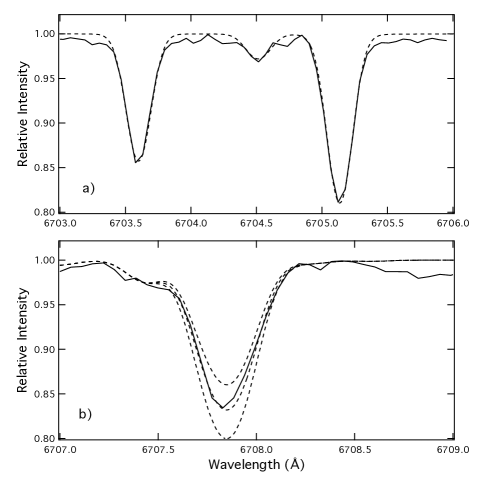
Figure 1: The observed spectrum of HD 74156 is shown as a solid curve in each panel. Best-fit synthetic spectrum of the region containing the two Fe I lines used to determine vsini is shown as a dashed curve (panel a). Best-fit and $\pm$ 0.1 dex Li abundance syntheses are shown as dashed curves (panel b).

Figure 2: Differences between the spectroscopic and photometric log g values for all the stars analyzed in the present work.

Table 1: Parameters determined from our spectroscopic analyses of 53 SWPs in columns 3 to 8. Derived parameters based on stellar isochrones are given in columns 9 to 11.

Star		Teff	log g	$\zeta_{\rm t}$ (km s-1)	[Fe/H]	log $\epsilon$(Li)	vsini (km s-1)	mass (M⊙)	log g	age (Gyr)
HD	HIP	$\pm$	$\pm$	$\pm$	$\pm$	$\pm$	$\pm$	$\pm$	$\pm$	$\pm$
3651	3093	5143	4.30	0.8	0.184	-0.30	1.6	0.89	4.49	5.3
		38	0.07	0.09	0.024	0.05	0.5	0.03	0.02	4.5
4113	3391	5626	4.30	0.9	0.240	0.53	3.5	1.00	4.31	6.6
		31	0.06	0.08	0.022	0.06	0.4	0.03	0.05	3.1
11506	8770	6136	4.42	1.5	0.323	2.71	6.0	1.21	4.28	1.6
		50	0.06	0.09	0.036	0.06	0.5	0.02	0.03	1.0
11964	9094	5265	3.74	1.0	0.121	1.19	3.3	1.10	3.87	7.6
		30	0.05	0.07	0.020	0.06	0.5	0.03	0.03	0.6
16175	12191	5930	4.02	1.4	0.310	2.45	5.5	1.25	4.04	3.8
		38	0.05	0.05	0.029	0.06	0.5	0.05	0.04	0.7
17156	13192	5993	4.04	1.4	0.181	2.40	5.0	1.16	4.22	3.5
		47	0.03	0.07	0.035	0.06	0.8	0.03	0.05	1.2
20367	15323	6090	4.34	1.4	0.105	2.67	$<$3.3	1.14	4.35	1.3
		40	0.04	0.10	0.030	0.06	0.2	0.03	0.03	1.1
20782	15527	5760	4.36	1.2	-0.048	0.64	3.0	0.96	4.32	7.9
		26	0.04	0.09	0.019	0.07	0.6	0.03	0.04	3.1
23596	17747	6045	4.18	1.2	0.286	2.77	4.2	1.22	4.18	3.1
		56	0.14	0.07	0.042	0.08	0.6	0.02	0.04	0.5
27063	19925	5750	4.39	1.2	0.065	1.62	$<$2.0	1.00	4.44	2.2
		20	0.02	0.06	0.020	0.05	0.7	0.03	0.03	2.1
33283	23889	5988	4.00	1.5	0.309	2.16	5.0	1.34	3.98	3.2
		21	0.04	0.03	0.016	0.05	0.7	0.06	0.05	0.5
33564	25110	6554	4.49	2.0	0.211	2.17	14.5	1.34	4.26	0.5
		93	0.05	0.2	0.063	0.09	0.5	0.02	0.02	0.3
37605	26664	5270	4.26	1.0	0.265	$<$-0.12	3.5	0.91	4.47	5.1
		47	0.07	0.07	0.033	0.05	0.7	0.03	0.03	4.2
43691	30057	6144	4.05	1.5	0.268	1.98	6.0	1.27	4.15	2.5
		34	0.05	0.07	0.026	0.06	1.0	0.04	0.06	0.5
45350	30860	5523	4.10	1.0	0.292	$<$0.01	1.6	0.98	4.19	10.1
		30	0.04	0.05	0.023	0.05	0.6	0.02	0.04	1.2
45652	30905	5232	4.20	0.9	0.286	$<$-0.64	3.5	0.91	4.46	6.2
		48	0.07	0.06	0.032	0.08	0.5	0.03	0.03	4.4
47186	31540	5630	4.27	1.1	0.252	$<$-0.40	4.0	1.00	4.31	6.9
		38	0.06	0.06	0.030	0.06	0.5	0.03	0.04	2.8
49674	32916	5590	4.38	1.0	0.325	0.39	0.9	0.99	4.38	4.9
		31	0.03	0.08	0.021	0.05	0.5	0.03	0.05	3.7
50499	32970	6045	4.31	1.5	0.312	2.61	4.2	1.19	4.23	2.9
		27	0.03	0.05	0.020	0.06	0.8	0.02	0.03	0.9
60532	36795	6121	3.73	2.2	-0.250	1.63	8.0	1.37	3.72	2.8
		85	0.05	0.25	0.060	0.08	0.6	0.04	0.03	0.2
66428	39417	5686	4.26	1.0	0.324	$<$0.58	$<$0.5	1.02	4.31	5.5
		35	0.05	0.06	0.026	0.09	0.4	0.03	0.06	3.1
69830	40693	5413	4.52	1.0	-0.006	0.65	$<$0.5	0.90	4.49	4.4
		25	0.07	0.11	0.019	0.05	0.5	0.03	0.02	3.9
70573		5807	4.35	1.8	-0.049	2.75	13.5
		85	0.08	0.16	0.064	0.09	0.5
70642	40952	5671	4.40	1.0	0.220	0.75	0.5	1.01	4.42	2.4
		31	0.04	0.09	0.021	0.09	0.5	0.03	0.03	2.3
72659	42030	5883	4.08	1.3	-0.022	2.19	$<$2.2	1.05	4.15	7.0
		37	0.08	0.07	0.029	0.06	0.5	0.03	0.04	1.2
74156	42723	6009	4.12	1.5	0.064	2.41	4.2	1.19	4.08	4.3
		40	0.04	0.08	0.030	0.06	0.5	0.04	0.04	0.8
75898	43674	5966	3.98	1.3	0.249	2.51	5.0	1.22	4.11	3.8
		55	0.07	0.08	0.042	0.07	0.5	0.05	0.06	0.7
80606	45982	5507	4.33	1.0	0.339	$<$0.17	2.0	0.98	4.33	5.5
		32	0.07	0.06	0.022	0.07	0.4	0.06	0.15	4.6
81040	46076	5798	4.55	1.2	-0.033	1.92	3.0	0.97	4.46	2.1
		26	0.03	0.07	0.020	0.06	0.7	0.03	0.02	2.0
86081	48711	6000	4.16	1.6	0.183	1.85	5.0	1.16	4.25	2.9
		27	0.04	0.04	0.020	0.05	0.6	0.04	0.07	1.6

Table 2: continued

Star		Teff	log g	$\zeta_{\rm t}$ (km s-1)	[Fe/H]	log $\epsilon$(Li)	vsini (km s-1)	mass (M⊙)	log g	age (Gyr)
HD	HIP	$\pm$	$\pm$	$\pm$	$\pm$	$\pm$	$\pm$	$\pm$	$\pm$	$\pm$
88133	49813	5320	3.69	1.1	0.325	1.56	2.2	1.97	3.33	1.2
		36	0.05	0.06	0.024	0.07	0.8	0.10	0.06	0.2
89307	50473	5961	4.37	1.5	-0.120	2.10	2.9	1.01	4.35	4.9
		34	0.03	0.07	0.024	0.06	0.5	0.04	0.04	2.9
107148	60081	5763	4.32	1.1	0.316	1.06	0.7	1.05	4.31	4.6
		13	0.03	0.04	0.010	0.05	0.5	0.03	0.05	2.5
114729	64459	5778	4.04	1.6	-0.320	1.73	2.3	0.94	4.02	10.9
		31	0.06	0.10	0.010	0.06	0.6	0.01	0.03	0.5
114762	64426	5766	3.87	1.6	-0.779	1.85	$<$1.8	0.82	4.23	12.6
		51	0.04	0.22	0.040	0.07	0.4	0.02	0.15	0.1
117207	65808	5618	4.19	1.0	0.259	$<$0.03	$<$1.1	0.99	4.31	7.1
		30	0.04	0.07	0.023	0.05	0.5	0.03	0.04	2.8
118203	66192	5827	3.95	1.4	0.209	2.47	5.0	1.26	3.97	4.0
		25	0.03	0.05	0.020	0.05	0.6	0.06	0.05	0.7
132406	73146	5727	4.10	1.3	0.111	1.09	4.0	1.01	4.26	7.4
		32	0.03	0.08	0.024	0.06	0.7	0.03	0.05	2.2
136118	74948	6248	4.21	1.8	-0.016	2.18	7.5	1.21	4.17	3.1
		45	0.03	0.09	0.031	0.06	0.5	0.02	0.03	0.5
141937	77740	5855	4.37	1.2	0.119	2.21	$<$1.9	1.05	4.40	1.8
		20	0.03	0.06	0.016	0.05	0.5	0.03	0.03	1.7
147513	80337	5886	4.46	1.2	0.073	1.89	$<$1.7	1.03	4.44	1.4
		22	0.03	0.06	0.017	0.05	0.7	0.02	0.02	1.2
149026	8038	6131	4.22	1.5	0.307	2.31	6.0	1.24	4.19	2.4
		35	0.05	0.06	0.026	0.06	0.5	0.03	0.05	0.7
149661	81300	5184	4.41	0.8	0.051	-0.20	$<$2.2	0.86	4.53	4.5
		39	0.06	0.08	0.024	0.05	0.3	0.02	0.02	4.1
150706	80902	5883	4.39	1.2	-0.041	2.46	4.5	1.01	4.42	2.3
		33	0.05	0.07	0.025	0.06	0.6	0.04	0.03	2.1
152391	82588	5450	4.51	1.2	0.003	1.11	3.8	0.90	4.50	3.9
		31	0.07	0.07	0.022	0.06	0.5	0.03	0.02	3.5
154345	83389	5358	4.26	0.8	-0.105	$<-0.29$	$<$1.5	0.88	4.49	6.1
		51	0.08	0.10	0.038	0.05	0.3	0.03	0.02	4.7
156846	84856	6068	3.98	1.5	0.196	1.07	5.0	1.37	3.98	2.8
		33	0.07	0.06	0.024	0.05	0.4	0.04	0.03	0.4
164922	88348	5281	4.25	0.8	0.205	$<$0.23	$<$2.0	0.91	4.42	7.6
		36	0.07	0.09	0.026	0.08	0.5	0.03	0.03	4.0
165401	88622	5790	4.62	1.5	-0.416	0.75	4.5	0.86	4.42	8.6
		31	0.05	0.12	0.023	0.07	0.5	0.02	0.03	3.0
168746	90004	5549	4.35	1.1	-0.093	0.72	$<$0.5	0.91	4.36	10.0
		26	0.03	0.06	0.022	0.05	0.5	0.02	0.03	1.9
183263	95740	5943	4.37	1.4	0.300	2.29	1.8	1.13	4.28	3.0
		35	0.04	0.06	0.026	0.06	0.4	0.03	0.05	1.7
185269	96507	5997	3.94	1.7	0.101	2.21	6.0	1.32	3.96	3.4
		47	0.03	0.07	0.036	0.06	0.5	0.05	0.03	0.5
188015	97769	5684	4.26	1.0	0.275	$<$-0.10	$<$0.5	1.02	4.27	6.6
		31	0.08	0.07	0.025	0.05	0.5	0.03	0.05	2.4
189733	98505	4952	4.26	0.9	0.010	$<$-0.30	4.5	0.81	4.56	4.8
		64	0.12	0.08	0.036	0.14	0.5	0.02	0.02	4.0
190360	98767	5500	4.19	1.0	0.227	0.41	2.5	0.96	4.28	9.6
		36	0.06	0.10	0.028	0.06	0.5	0.02	0.03	1.7
196885	101966	6288	4.36	1.8	0.210	2.58	8.0	1.26	4.27	1.0
		61	0.04	0.10	0.043	0.06	0.5	0.02	0.03	0.7
208487	108375	6200	4.67	1.8	0.085	2.51	4.5	1.16	4.34	1.0
		65	0.06	0.14	0.047	0.07	0.5	0.03	0.03	0.9
216770	113238	5316	4.22	0.95	0.293	0.62	1.2	0.92	4.45	5.6
		47	0.09	0.09	0.033	0.10	0.4	0.03	0.03	4.3
219828	115100	5861	4.21	1.5	0.175	2.17	4.5	1.16	4.1	4.9
		38	0.03	0.08	0.029	0.06	0.5	0.05	0.05	0.9
224693	118319	6024	4.23	1.6	0.270	1.89	5.5	1.31	4.03	3.1
		41	0.04	0.07	0.031	0.06	0.5	0.06	0.07	0.5
	14810	5501	4.32	1.0	0.274	0.92	$<$1.5	0.95	4.35	7.2
		38	0.05	0.10	0.027	0.06	0.5	0.03	0.06	4.6

Table 3: Parameters determined from our spectroscopic reanalyses of the SWPs included in our previous papers. Note: the two spectra of HD 8574 were obtained on different runs. HD 170469 is from the April 2002 run. Columns are the same as in Table 1.

Star		Teff	log g	$\zeta_{\rm t}$ (km s-1)	[Fe/H]	log $\epsilon$(Li)	vsini (km s-1)	mass (M⊙)	log g	age (Gyr)
HD	HIP	$\pm$	$\pm$	$\pm$	$\pm$	$\pm$	$\pm$	$\pm$	$\pm$	$\pm$
4203	3502	5535	4.04	1.1	0.371	$<$0.50	1.7	1.00	4.14	9.8
		30	0.04	0.04	0.023	0.06	0.4	0.03	0.07	1.2
4208	3479	5638	4.46	1.1	-0.232	$<$0.44	$<$0.5	0.89	4.49	4.7
		25	0.04	0.14	0.020	0.07	0.5	0.03	0.03	4.0
6434	5054	5744	4.29	1.4	-0.588	0.70	$<$1.0	0.84	4.38	11.3
		45	0.03	0.24	0.034	0.07	0.5	0.01	0.01	0.3
8574(a)	6643	6040	4.10	1.5	-0.040	2.48	4.5	1.10	4.17	5.3
		33	0.02	0.07	0.026	0.06	0.5	0.03	0.04	1.0
8574(b)	6643	6090	4.26	1.7	-0.017	2.43	4.5	1.13	4.20	4.4
		35	0.04	0.10	0.025	0.06	0.5	0.03	0.04	0.9
9826	7513	6170	4.00	1.8	0.084	2.16	9.5	1.26	4.11	3.1
		48	0.08	0.10	0.037	0.06	0.4	0.03	0.03	0.5
12661	9683	5670	4.31	1.0	0.376	1.92	1.2	1.01	4.35	4.6
		27	0.03	0.06	0.021	0.06	0.4	0.03	0.04	3.1
16141	12048	5770	4.06	1.2	0.163	1.34	1.9	1.10	4.10	6.2
		25	0.04	0.05	0.019	0.06	0.8	0.03	0.04	1.1
19994	14954	6190	4.16	1.8	0.207	1.83	8.0	1.33	4.08	2.5
		45	0.04	0.08	0.032	0.07	0.3	0.01	0.03	0.3
22049	16537	5000	4.30	0.9	-0.088	0.36	3.2	0.80	4.57	4.8
		41	0.09	0.07	0.024	0.07	0.4	0.02	0.02	3.9
28185	20723	5605	4.36	1.0	0.233	0.63	2.0	0.99	4.31	7.3
		32	0.05	0.06	0.022	0.07	0.3	0.03	0.05	3.0
37124	26381	5520	4.30	1.0	0.228	0.35	$<$2.0	0.92	4.36	10.2
		40	0.09	0.14	0.023	0.06	0.4	0.01	0.02	1.3
46375	31246	5195	4.34	0.8	0.297	0.02	$<$1.5	0.90	4.41	9.8
		36	0.05	0.09	0.021	0.06	0.6	0.01	0.02	2.1
50554	33212	6056	4.42	1.4	0.006	2.44	3.5	1.09	4.39	1.4
		28	0.02	0.07	0.006	0.02	0.5	0.03	0.03	1.2
68988	40687	5901	4.32	1.2	0.334	2.02	3.0	1.10	4.37	4.5
		34	0.03	0.06	0.025	0.06	0.4	0.03	0.03	1.5
75289	43177	6174	4.46	1.5	0.290	2.66	4.2	1.20	4.31	1.0
		30	0.08	0.05	0.022	0.06	0.4	0.02	0.02	0.7
80606	45982	5507	4.33	1.0	0.339	$<$0.17	2.0	0.98	4.33	5.5
		32	0.07	0.06	0.022	0.07	0.4	0.06	0.15	4.6
82943	47007	6012	4.43	1.4	0.295	2.39	$<$1.5	1.14	4.35	1.2
		35	0.04	0.10	0.025	0.06	0.4	0.02	0.02	1.0
89744	50786	6237	3.88	2.0	0.170	1.88	9.0	1.48	3.93	2.2
		50	0.04	0.10	0.035	0.07	0.5	0.02	0.03	0.2
95128	53721	5867	4.26	1.3	0.025	1.66	2.9	1.03	4.26	6.5
		21	0.02	0.06	0.016	0.05	0.5	0.03	0.02	1.6
106252	59610	5839	4.23	1.2	-0.083	1.53	$<$1.5	0.97	4.32	7.2
		31	0.05	0.06	0.023	0.06	0.6	0.03	0.04	3.0
114762	64426	5766	3.87	1.6	-0.779	1.85	$<$1.8	0.82	4.23	12.6
		51	0.04	0.22	0.040	0.07	0.4	0.02	0.15	0.1
114783	64457	5000	4.32	0.8	0.090	$<$0.01	$<$1.0	0.84	4.54	5.2
		57	0.22	0.10	0.021	0.05	0.4	0.02	0.02	4.3
117176	65721	5502	3.88	1.2	-0.070	1.78	2.7	1.07	3.90	8.1
		17	0.02	0.04	0.013	0.05	0.4	0.01	0.03	0.3
120136	67275	6342	3.92	1.8	0.195	2.14	13.5	1.29	4.21	1.6
		100	0.10	0.2	0.070	0.10	0.5	0.02	0.03	0.6
130322	72339	5368	4.46	0.9	0.080	0.61	$<$1.7	0.90	4.49	4.2
		31	0.05	0.08	0.020	0.06	0.3	0.03	0.03	3.8
134987	74500	5687	4.17	1.1	0.299	0.94	$<$2.0	1.03	4.23	7.4
		35	0.05	0.05	0.026	0.06	0.2	0.02	0.04	1.5
136118	74948	6248	4.21	1.8	-0.016	2.18	7.5	1.21	4.17	3.1
		45	0.03	0.09	0.031	0.06	0.5	0.02	0.03	0.5
141937	77740	5855	4.37	1.2	0.119	2.21	$<$1.9	1.05	4.40	1.8
		20	0.03	0.06	0.016	0.05	0.5	0.03	0.03	1.7
149661	81300	5184	4.41	0.8	0.051	-0.20	$<$2.2	0.86	4.53	4.5
		39	0.06	0.08	0.024	0.05	0.3	0.02	0.02	4.1

Table 4: continued

Star		Teff	log g	$\zeta_{\rm t}$ (km s-1)	[Fe/H]	log $\epsilon$(Li)	vsini (km s-1)	mass (M⊙)	log g	age (Gyr)
HD	HIP	$\pm$	$\pm$	$\pm$	$\pm$	$\pm$	$\pm$	$\pm$	$\pm$	$\pm$
152391	82588	5450	4.51	1.2	0.003	1.11	3.8	0.90	4.50	3.9
		31	0.07	0.07	0.022	0.06	0.5	0.03	0.02	3.5
165401	88622	5790	4.62	1.5	-0.416	0.75	4.5	0.86	4.42	8.6
		31	0.05	0.12	0.023	0.07	0.5	0.02	0.03	3.0
168443	89844	5524	3.99	1.0	0.083	0.43	2.5	1.01	4.03	10.1
		24	0.05	0.05	0.018	0.05	0.4	0.02	0.03	0.6
168746	90004	5549	4.35	1.1	-0.093	0.72	$<$0.5	0.91	4.36	10.1
		26	0.03	0.06	0.022	0.05	0.5	0.02	0.03	1.9
170469	90593	5766	4.25	1.2	0.306	1.31	$<$1.7	1.07	4.23	5.8
		31	0.03	0.04	0.023	0.12	0.8	0.03	0.06	1.9
190228	98714	5235	3.60	1.0	-0.267	1.19	2.0	1.17	3.68	5.3
		22	0.05	0.09	0.017	0.05	0.6	0.04	0.04	0.7
195019	100970	5780	4.15	1.3	0.061	1.27	$<$2.0	1.05	4.10	7.6
		19	0.02	0.03	0.015	0.05	0.6	0.02	0.04	0.9
202206	104903	5709	4.39	1.1	0.322	1.40	$<$1.0	1.02	4.42	2.1
		26	0.03	0.05	0.019	0.05	0.5	0.03	0.03	1.9

Table 5: Parameters determined for the comparison stars. Columns are the same as in Table 1.

Star		Teff	log g	$\zeta_{\rm t}$ (km s-1)	[Fe/H]	log $\epsilon$(Li)	vsini (km s-1)	mass (M⊙)	log g	age (Gyr)
HD	HIP	$\pm$	$\pm$	$\pm$	$\pm$	$\pm$	$\pm$	$\pm$	$\pm$	$\pm$
S4N
4614	3821	5904	4.32	1.2	-0.246	2.03	$<$2.5	0.94	4.34	8.2
		32	0.03	0.11	0.024	0.06	0.5	0.03	0.03	2.4
9826	7513	6239	4.19	1.7	0.145	2.20	9.5	1.29	4.14	2.4
		37	0.03	0.06	0.026	0.06	0.4	0.02	0.03	0.3
10307	7918	5847	4.15	1.1	0.041	1.71	$<$3.5	1.03	4.31	5.6
		25	0.04	0.07	0.019	0.06	0.7	0.03	0.04	2.4
13974	10644	5799	4.29	0.8	-0.439	2.21	$<$1.5	0.87	4.35	10.
		70	0.09	0.50	0.050	0.08	0.1	0.01	0.02	1.1
16895	12777	6329	4.32	1.6	0.057	2.80	9.0	1.22	4.30	1.0
		37	0.02	0.08	0.026	0.06	0.5	0.02	0.02	0.8
17206	12843	6504	4.44	1.6	0.279	1.94	27.	1.25	4.31	0.5
		211	0.16	0.30	0.150	0.18	1.0	0.03	0.02	0.4
17925	13402	5060	4.25	1.1	0.120	2.27	6.0	0.85	4.53	4.8
		79	0.16	0.30	0.040	0.14	0.5	0.02	0.02	4.1
19373	14632	6008	4.33	1.3	0.151	2.27	4.5	1.16	4.21	3.8
		33	0.03	0.07	0.023	0.06	0.5	0.02	0.03	0.9
20010	14879	6170	3.93	1.7	-0.206	1.86	5.0	1.25	3.94	3.8
		35	0.02	0.09	0.025	0.06	0.6	0.04	0.03	0.7
20630	15457	5749	4.51	1.1	0.078	1.75	5.5	1.00	4.46	1.7
		26	0.05	0.05	0.018	0.06	0.5	0.03	0.02	1.7
22049	16537	5032	4.30	0.6	-0.012	0.05	2.5	0.82	4.57	3.2
		48	0.08	0.12	0.021	0.09	0.5	0.02	0.02	3.6
22484	16852	5996	3.97	1.4	-0.045	2.10	4.5	1.15	4.06	5.3
		26	0.01	0.06	0.019	0.05	0.8	0.04	0.03	1.0
30495	22263	5823	4.42	1.1	0.042	2.29	4.0	1.01	4.44	2.0
		26	0.05	0.07	0.019	0.05	0.5	0.03	0.02	1.8
34411	24813	5858	4.14	1.1	0.103	1.95	$<$2.0	1.06	4.23	6.0
		19	0.03	0.09	0.016	0.05	0.5	0.03	0.03	1.3
39587	27913	5974	4.43	1.3	0.018	2.74	9.0	1.05	4.43	1.2
		33	0.05	0.06	0.025	0.06	0.5	0.03	0.02	1.1
61421	37279	6593	3.90	1.8	0.022	$<$0.81	5.0	1.47	3.99	1.8
		50	0.01	0.12	0.032	0.14	0.6	0.02	0.02	0.1
69830	40693	5382	4.34	0.8	-0.018	0.75	3.5	0.89	4.49	5.0
		25	0.09	0.12	0.017	0.06	0.5	0.03	0.03	4.2
72905	42438	5873	4.44	1.5	-0.043	2.65	10.0	1.00	4.44	2.1
		34	0.05	0.07	0.026	0.06	0.6	0.03	0.02	1.9
82328	46853	6336	3.72	1.7	-0.140	3.09	8.5	1.44	3.84	2.4
		62	0.05	0.13	0.042	0.07	0.5	0.05	0.03	0.3
90839	51459	6146	4.37	1.5	-0.061	2.65	$<$1.5	1.10	4.36	1.8
		33	0.02	0.15	0.024	0.06	0.8	0.03	0.03	1.5
95128	53721	5842	4.13	1.1	0.025	1.61	$<$2.0	1.02	4.24	7.0
		31	0.05	0.09	0.024	0.06	0.5	0.03	0.04	1.6
102870	55757	6111	4.00	1.4	0.160	1.86	4.0	1.30	4.08	3.0
		28	0.05	0.06	0.021	0.05	0.5	0.03	0.03	0.4
109358	61317	5806	4.16	1.1	-0.220	1.50	$<$2.5	0.92	4.32	10.
		24	0.07	0.08	0.019	0.05	0.5	0.02	0.03	1.7
114710	64394	6021	4.37	1.2	0.083	2.50	4.3	1.10	4.38	1.4
		21	0.05	0.04	0.015	0.05	0.7	0.03	0.02	1.2
115617	64924	5533	4.29	0.9	0.010	$<$0.10	2.2	0.93	4.42	6.8
		19	0.03	0.06	0.013	0.06	0.5	0.03	0.03	3.9
121370	67927	6085	3.70	1.7	0.283	1.57	13.0	1.60	3.77	2.0
		54	0.10	0.07	0.041	0.07	0.5	0.03	0.20	0.1
131156	72659	5595	4.70	1.1	-0.075	2.24	5.0	0.90	4.50	3.3
		24	0.06	0.06	0.015	0.06	0.6	0.03	0.02	2.8
133640	73695	5848	4.32	0.9	-0.186	1.95	$<$3.5	0.95	4.24	9.9
		33	0.03	0.11	0.025	0.06	0.5	0.02	0.03	1.2
141004	77257	5869	4.00	1.1	0.010	1.73	3.2	1.05	4.15	7.1
		32	0.09	0.08	0.025	0.06	0.5	0.02	0.03	1.1

Table 6: continued

Star		Teff	log g	$\zeta_{\rm t}$ (km s-1)	[Fe/H]	log $\epsilon$(Li)	vsini (km s-1)	mass (M⊙)	log g	age (Gyr)
HD	HIP	$\pm$	$\pm$	$\pm$	$\pm$	$\pm$	$\pm$	$\pm$	$\pm$	$\pm$
142860	78072	6209	3.91	1.4	-0.160	2.03	11.0	1.15	4.12	4.9
		55	0.08	0.07	0.037	0.07	0.5	0.04	0.03	0.9
146233	79672	5753	4.22	1.0	0.051	1.43	2.7	1.00	4.39	3.9
		37	0.09	0.07	0.030	0.07	0.6	0.04	0.04	3.1
150680	81693	5827	3.79	1.4	0.098	$<$0.64	4.5	1.41	3.74	2.9
		18	0.03	0.05	0.015	0.07	0.5	0.03	0.03	0.2
157214	84862	5736	4.39	0.9	-0.315	$<$0.07	1.9	0.89	4.31	11.
		37	0.05	0.18	0.027	0.05	0.6	0.01	0.01	0.6
160269	86036	6026	4.58	1.2	0.078	2.50	5.0	1.10	4.39	1.3
		41	0.04	0.10	0.030	0.06	0.5	0.03	0.02	1.1
165896	88937	6206	4.38	1.8	-0.525	2.26	9.0	0.94	4.20	8.7
		85	0.05	0.60	0.055	0.08	0.5	0.03	0.03	1.3
222368	116771	6104	3.87	1.4	-0.120	2.09	7.5	1.17	4.05	4.9
		61	0.07	0.15	0.050	0.07	0.5	0.04	0.03	0.9
APR02
69897	40843	6232	4.12	1.7	-0.255	2.57	5.7	1.08	4.18	5.5
		62	0.03	0.18	0.041	0.05	0.7	0.03	0.03	0.8
84737	48113	5934	4.16	1.3	0.163	2.28	3.0	1.17	4.13	4.5
		33	0.03	0.07	0.026	0.06	0.6	0.04	0.03	0.8
86728	49081	5753	4.30	1.1	0.260	1.27	3.3	1.05	4.32	4.7
		41	0.04	0.10	0.030	0.06	0.5	0.03	0.02	1.1
99491	55846	5415	4.37	1.1	0.303	0.83	$<$1.4	0.94	4.44	4.8
		39	0.05	0.08	0.027	0.07	0.7	0.03	0.03	4.0
101501	56997	5530	4.46	1.0	-0.002	0.86	$<$2.2	0.93	4.41	4.8
		24	0.03	0.08	0.017	0.05	0.4	0.06	0.15	4.2
102634	57629	6342	4.24	1.8	0.219	2.40	6.6	1.31	4.19	1.6
		59	0.03	0.11	0.042	0.05	0.4	0.02	0.03	0.5
102870	57757	6180	4.15	1.4	0.213	1.94	4.0	1.30	4.11	2.5
		36	0.05	0.07	0.026	0.06	0.6	0.01	0.02	0.3
109358	61317	5887	4.34	1.5	-0.198	1.63	$<$2.5	0.95	4.33	8.1
		26	0.03	0.11	0.021	0.05	0.6	0.03	0.04	2.7
114710	64394	6020	4.35	1.3	0.083	2.40	4.4	1.10	4.37	1.5
		28	0.02	0.06	0.020	0.05	0.6	0.03	0.03	1.3
115383	64792	6100	4.28	1.5	0.192	2.69	7.1	1.19	4.27	2.0
		35	0.06	0.05	0.026	0.06	0.3	0.02	0.03	1.1
120066	67246	5862	4.12	1.4	0.081	2.67	3.5	1.11	4.11	6.0
		25	0.03	0.06	0.020	0.05	0.5	0.03	0.04	1.0
122652	68593	6199	4.46	1.4	0.063	2.69	4.2	1.15	4.36	0.9
		34	0.04	0.08	0.025	0.05	0.5	0.02	0.02	0.7
134044	73941	6290	4.48	1.6	0.131	2.70	4.4	1.21	4.32	0.7
		38	0.05	0.08	0.026	0.05	0.6	0.02	0.02	0.6
135101A	74432	5665	4.14	1.3	0.054	0.95	$<$1.8	0.90	4.27	9.2
		24	0.04	0.04	0.019	0.11	0.7	0.02	0.04	1.9
145825	79578	5795	4.43	1.2	0.054	1.85	$<$1.4	1.01	4.44	1.9
		25	0.03	0.06	0.019	0.05	1.0	0.03	0.03	1.8
147044	79862	5852	4.42	1.2	-0.016	2.06	$<$2.0	1.01	4.37	3.0
		41	0.08	0.10	0.030	0.06	0.8	0.04	0.04	3.0
150433	81681	5678	4.45	1.2	-0.326	0.91	$<$1.2	0.87	4.39	10.
		32	0.07	0.11	0.025	0.10	0.7	0.02	0.02	1.4
153458	83181	5841	4.51	1.2	0.133	2.14	$<$0.5	1.05	4.40	1.7
		21	0.03	0.07	0.016	0.06	0.8	0.03	0.03	1.7
157347	85042	5709	4.48	1.1	0.071	1.01	$<$0.9	0.99	4.40	4.2
		26	0.05	0.07	0.019	0.05	0.9	0.04	0.04	3.3
159222	85810	5851	4.41	1.3	0.155	1.93	3.3	1.07	4.39	1.9
		20	0.02	0.06	0.016	0.06	0.8	0.03	0.03	1.7
161555	86985	5817	4.02	1.4	0.116	2.44	$<$2.9	1.15	4.04	5.5
		38	0.05	0.06	0.030	0.05	0.4	0.04	0.05	1.0
162826	87382	6219	4.38	1.5	0.075	2.55	3.6	1.19	4.28	1.7
		37	0.03	0.07	0.026	0.05	0.5	0.03	0.03	1.1

Table 7: continued

Star		Teff	log g	$\zeta_{\rm t}$ (km s-1)	[Fe/H]	log $\epsilon$(Li)	vsini (km s-1)	mass (M⊙)	log g	age (Gyr)
HD	HIP	$\pm$	$\pm$	$\pm$	$\pm$	$\pm$	$\pm$	$\pm$	$\pm$	$\pm$
164595	88194	5698	4.30	1.1	-0.065	0.96	$<$0.5	0.94	4.38	6.8
		25	0.06	0.06	0.019	0.09	0.3	0.04	0.04	4.0
171067	90864	5644	4.53	1.1	-0.015	0.73	$<$0.7	0.95	4.46	3.4
		21	0.05	0.10	0.017	0.11	0.7	0.03	0.03	3.2

For the 31 SWPs in common between the present SWP sample and our previous studies, the mean difference in T_eff is only 15 K, while the mean $\sigma$ for T_eff is reduced from 43 K to 35 K. This demonstrates that our revised procedure for measuring EWs gives more precise T_eff values than the manual procedure we had employed in our previous studies, and it doesn’t introduce significant systematic error.

Originally, the SWP sample in the present study consisted of 90 stars. However, for 5 of these stars (HD 33564, HD 114762, HD 136118, HD 141937 and HD 168443) the minimum masses of the plants are close to the brown dwarf limit (11 M_J), and in some cases there is additional evidence that the true planet masses are beyond this limit. For these reasons, we transferred these stars to the comparison sample, leaving 85 stars in the SWPs sample.

We also determined age, mass and log g for each star from stellar isochrones. In particular, we employed our T_eff and [Fe/H] values with M_v calculated from the new reduction of the Hipparcos parallaxes (van Leeuwen, 2007) with a Bayesian parameter estimation method (da Silva et al., 2006). The mean difference between our spectroscopic log g values and the parallax derived (photometric) values is -0.02 $\pm$ 0.12 dex. However, as can be seen in Figure 2 there is a significant trend present among the SWPs in the sense that the spectroscopic values are smaller than the isochrone ones; the trend is not significant if we exclude the cooler stars. If we restrict the comparison to T${}_{\rm eff}>5650$ K, then the difference is 0.00 $\pm$ 0.10 dex. This gives us confidence that the analysis results do not have systematic errors more than a few hundredths of a dex for this temperature range.

We show the Li abundances in Figure 3. The dividing/cutoff line between upper limits and detections of Li is about half a dex lower in the present sample compared to that in our previous study (Gonzalez, 2008). We positioned the dividing line such that most stars with upper limits fall below it, and most stars with detections fall above it.

The number of comparison stars is very limited below about T${}_{\rm eff}=5650$ K, and the hottest SWP has a T_eff value just under 6350 K. Given this, we limit our comparison of Li abundances between SWPs and stars without planets to T${}_{\rm eff}=$ 5650 to 6350 K. This compares to a T_eff range of 5550 to 6250 K in Gonzalez (2008). In addition, for this choice of T_eff all the SWP and comparison stars fall above the Li dividing/cutoff line.

Figure 3: Li abundances versus T_eff for SWPs (dots) and stars without planets (open circles). Upper limits on the Li abundance are shown for SWPs (filled squares) and stars without planets (open squares). The upper limit cutoff for the present data set is shown as a dashed line; the corresponding cutoff from Gonzalez (2008) is shown as a dotted line.

We plot our vsini estimates against T_eff in Figure 4. In this case, the stars with detected vsini are mixed over a large range in vsini with stars that have upper limits. For this reason, we set our vsini cutoff line rather high for the next step in the analysis. We also prepared a separate dataset with the vsini estimates of Valenti & Fischer (2005) in place of our vsini estimates; we plot these data in Figure 5.

For the 71 stars in the present study with vsini detections that overlap with the sample of Valenti & Fischer (2005), the mean difference in vsini is 0.1 $\pm$ 0.5 km s^-1.

Figure 4: vsini versus T_eff; symbols have the same meanings as in Figure 3. The upper limit cutoff is shown as a dashed line curve in this plot, but it is actually linear.

Figure 5: Same as Figure 4 but with vsini values from Valenti & Fischer (2005).

3 Comparison of Samples

In Gonzalez (2008) we introduced a new index, $\Delta_{1}$, which is a measure of the distance between two stars in T_eff-[Fe/H]-log g-M_v space. We calculated a weighted average Li abundance difference between a given SWP and all the comparison stars with $(\Delta_{1})^{-2}$ as the weight. We employ the same analysis here with our new samples.

One star in our SWP sample, HD 70573, lacks a Hipparcos parallax. Since the $\Delta_{1}$ index weighting scheme requires M_v, we removed this star from our sample at this stage of our analysis. The number of retained SWPs in the range T${}_{\rm eff}=$ 5650 to 6350 K is 50. In our comparison sample, 50 stars fall in this T_eff range, but one star has an upper limit on its Li abundance. We removed this star, leaving 49 stars in our comparison sample. This compares to 37 SWPs and 147 comparison stars over the range T${}_{\rm eff}=$ 5550 to 6250 K in Gonzalez (2008). We show the resulting weighted average Li abundance differences between the SWPs and comparison stars in Figure 6.

Figure 6: Weighted average Li abundance differences between SWPs and comparison stars analyzed in the present study.

3.1 Correcting for bias in Li

In order to test for possible bias in our method of sample comparison, we will revisit the Li abundance data from Gonzalez (2008). If the Li abundance deficits we have detected among the SWPs near solar temperature are real, then there should be no trend with temperature when the comparison stars are analyzed in the same way. To realize this test, we selected every other star from the 147 comparison stars in Gonzalez (2008) and treated them as if they were SWPs (”fake SWPs”), and we treated the remaining stars as comparison stars. We then calculated the weighted Li abundance differences as before (Figure 7a). Next, we exchanged the roles of the stars and repeated the analysis (Figure 7b). There is a clear trend evident in these results; the slopes of least-squares fits to the two datasets in Figure 7 are 6.4$\times 10^{\rm-4}$ and 8.9$\times 10^{\rm-4}$ dex K^-1, respectively. We adopt an average ”bias slope” value of 7.7$\times 10^{\rm-4}$ dex K^-1.

We plot in Figure 8a the weighted Li abundance differences for the SWPs from Gonzalez (2008), which differ from the data plotted in Figure 3b of that paper only in that the newly revised Hipparcos parallaxes have been used to calculate the $\Delta_{1}$ index instead of the outdated 1997 values. Next, we corrected these data for bias by subtracting the average bias slope value quoted above. The resulting data (Figure 8b) no longer display Li abundance excesses above $\sim 6000$ K, but the Li abundance deficits are still present between about 5800 and 5900 K; there are not enough SWP data below 5800 K to reach a conclusion in this temperature range.

We repeated these tests with the datasets in the present study and show the results in Figures 9 and 10. The slopes of the data in Figure 9 are 1.3$\times 10^{\rm-3}$ and 4.4$\times 10^{\rm-4}$ dex K^-1. We adopt an average bias slope value of 8.7$\times 10^{\rm-4}$ dex K^-1. After applying this bias correction, we find that stars near the solar temperature still display the largest Li abundance deficits, but stars at intermediate temperatures also display modest Li abundance excesses.

There are 12 SWPs and 7 comparison stars between 5700 and 5800 K in the present study. If we apply a simple statistical t hypothesis test to the Li abundances from these samples (keeping in mind that we are not correcting for differences in the parameters here), we find that we can reject the hypothesis that these two samples are drawn from the same parent population with about 93% confidence.

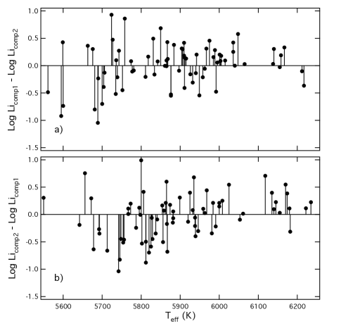
Figure 7: Weighted average Li abundance differences among the comparison stars from Gonzalez (2008). Roles of the comparison stars have been exchanged (panel b). See text for details.

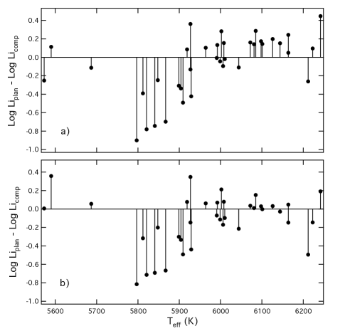
Figure 8: Weighted average Li abundance differences between SWPs and comparison stars for stars from Gonzalez (2008) (panel a). Li abundances corrected using the trends in Figure 7 (panel b).

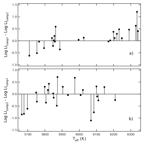
Figure 9: Same as Figure 7 but for comparison stars in the present study.

Figure 10: Same data as shown in Figure 6 but corrected for bias using average trend determined from data in Figure 9.

Figure 11: Weighted average vsini differences between two sets of comparison stars (like Figure 7). The vsini estimates are from Valenti & Fischer (2005).

Figure 12: Corrected weighted average vsini differences between SWPs and comparison stars from Valenti & Fischer (2005). The corrections have been applied from the trends in Figure 11.

3.2 Correcting for bias in vsini

We applied an analysis to the vsini data very similar to our analysis of the Li abundances in the last section. First, we show in Figure 11 the weighted vsini differences for the 596 comparison stars with vsini measurements in Valenti & Fischer (2005). As for the Li abundance differences, there is a trend present in the vsini differences; the slopes are 0.0055 and 0.0026 km s^-1 K^-1, respectively. We adopt an average value of 0.0041 km s^-1 K^-1. The corrected SWP weighted vsini differences are shown in Figure 12. The vsini deficits among the SWPs are evident in the plot between about 5700 and 5900 K.

Due to the small number of comparison stars with vsini determinations in the present study (33), we are not confident that we can derive a reliable bias trend from them. For this reason, we have adopted the mean bias trend from Figure 11 and applied it to the 40 SWP vsini differences based on the new vsini determinations in the present study (Figure 13a). In applying the bias correction to the vsini differences, we shifted the temperature scale of the Valenti & Fischer (2005) data to more closely match our temperature scale. The corresponding vsini differences for the 34 SWP Valenti & Fischer (2005) vsini values of the stars included in the present study are shown in Figure 13b. vsini deficits are evident in both plots for temperatures between about 5700 and 5900 K.

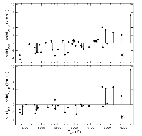
Figure 13: Weighted average vsini differences between SWPs and comparison stars versus T_eff. Panel (a) is based on vsini estimates in the present study. Panel (b) is based on vsini estimates from Valenti & Fischer (2005).

4 Discussion

Despite the presence of an unrecognized bias in the results presented in Gonzalez (2008), the general trend of weighted Li abundance differences with T_eff we determine is similar to the trend we presented in Figure 3b of that study. However, the data used in the present study show a rapid rise in Li abundance for SWPs with T${}_{\rm eff}>5850$, which is about 50 K cooler than the data in Gonzalez (2008). This is due to the fact that the T_eff scale adopted in Gonzalez (2008) is about 50 K higher than that adopted here. We consider the T_eff scale in the present study to be more accurate.

The trends of weighted vsini differences with T_eff are also similar to the trend we described in Gonzalez (2008). In that study, we found that vsini transitions between deficits and excesses just below T${}_{\rm eff}=$ 6100. In the present study we find that the transition occurs near 6000 K according to our vsini estimates and near 6100 K from the data of Valenti & Fischer (2005). This transition is not well constrained by the small number of SWPs with vsini estimates in the present study. Note, also, that the vsini values include a random component due to our ignorance of the inclination of a star’s rotation axis. For this reason, we need a larger sample to study the trend with vsini than we employed for the Li abundance analysis.

One side benefit of the samples prepared for this study is that we can now fairly compare the Sun’s Li abundance ($=0.96$ dex) to other stars. The Li abundance cutoff employed in Gonzalez (2008) was such that the Sun would have been excluded from the SWP sample due to its low Li abundance. Now we are prepared to answer the question, “Does the Sun’s Li abundance better fit the classification of a SWP or of a star without a planet, according to the distribution in Figure 10?” Applying the same analysis of the previous section to the Sun, we calculate a weighted solar Li abundance deficit of 0.70 dex relative to the 50 comparison stars. The average deficit for SWPs between 5700 and 5800 K This places the Sun squarely in the SWP category. Only 3 SWPs in Figure 10 have greater Li deficits than the Sun: HD 6434, HD 20782 and HD 165401.

The weighted solar vsini deficit is 1.25 km s^-1 relative to the larger Valenti & Fischer (2005) vsini comparison star dataset. The average vsini deficit for the SWPs with T_eff between 5700 and 6000 K is 0.9 $\pm$ 1.1 km s^-1. This also places the Sun squarely in the SWP category.

5 Conclusions

We confirm our previous findings from Gonzalez (2008) that the Li abundances of SWPs with T${}_{\rm eff}\leq 5800$ K are smaller than those of stars without detected planets; we also confirm that SWPs near $\sim 6000$ K have excess Li abundances. In addition, we confirm that SWPs have smaller vsini values than stars without detected planets for T_eff less than $\sim 6000$ K. These trends are robust, given that we employed different samples of SWPs and comparison stars in the two studies.

For the first time, we are able to compare the Sun’s Li abundance in a fair way to a sample of comparison stars. We find that its Li abundance is low compared to our sample of comparison stars, and it is comparable to the Li abundances of SWPs with similar T_eff values.

To improve on our analysis, it is important to determine Li abundances and vsini values for more SWPs and comparison stars with T${}_{\rm eff}>5500$ K. To be most useful, spectra should have S/N ratios $>300$ near 6700 Å.

References

- Allende Prieto et al. (2004) Allende Preito C., Barklem P. S., Lambert D. L., Cunha K., 2004, A&A, 420, 183
- Cayrel de Strobel (1996) Cayrel de Strobel, G., 1996, A&ARv, 7, 243
- da Silva et al. (2006) da Silva L., Girardi L., Pasquini L., Setiawan J., von der Luhe O., de Medeiros J. R., Hatzes A., Dollinger M. P., Weiss A., 2006, A&A, 458, 609
- Eggen (1998) Eggen O. J., 1998, AJ, 115, 2397
- Ghezzi et al. (2009) Ghezzi L., Cunha K., Smith V. V., Margheim S., Schuler S., de Araujo F. X., de al Reza R., 2009, ApJ, 698, 451
- Gonzalez (2008) Gonzalez G., 2008, MNRAS, 386, 928
- Gonzalez & Laws (2000) Gonzalez G., Laws C., 2000, AJ, 119, 390
- Gonzalez et al. (2001) Gonzalez G., Laws C., Tyagi S., Reddy B. E., 2001, AJ, 121, 432
- Gonzalez & Vanture (1998) Gonzalez G., Vanture A., 1998, A&A, 339, L29
- Grevesse & Sauval (1998) Grevesse N., Sauval A. J., 1998, SpaceSciRev, 347, 348
- Grevesse & Sauval (1999) Grevesse N., Sauval A. J., 1999, A&A, 347, 348
- Haywood (2001) Haywood M., 2001, MNRAS, 325, 1365
- Israelian et al. (2004) Israelian G., Santos N. C., Mayor M., Rebolo R., 2004, A&A, 414, 601
- Kurucz (1993) Kurucz R., 1993, ATLAS9 Stellar Atmosphere Programs and 2 km/s grid. Kurucz CD-ROM No. 13. Cambridge, Mass.: Smithsonian Astrophysical Observatory.
- Laws et al. (2003) Laws C., Gonzalez G., Walker K. M., Tyagi S., Dodsworth J., Snider K., Suntzeff N. B., 2003, AJ, 125, 2664
- van Leeuwen (2007) van Leeuwen F., 2007, Hipparcos, The New Reduction of the Raw Data, Springer
- Sneden (1973) Sneden C., 1973, Ph.D. thesis, University of Texas, Austin
- Stetson & Pancino (2008) Stetson P. B., Pancino E., 2008, PASP, 120, 1332
- Takeda & Kawanomoto (2005) Takeda Y., Kawanomoto S., 2005, PASJ, 57, 45
- Valenti & Fischer (2005) Valenti J., Fischer D. A., 2005, ApJS, 159, 141