Radii of Rapidly-Rotating Stars, with Application to Transiting-Planet Hosts

Abstract

The currently favored method for estimating radii and other parameters of transiting-planet host stars is to match theoretical models to observations of the stellar mean density $\rho_{*}$, the effective temperature $T_{\rm eff}$, and the composition parameter $[Z]$. This explicitly model-dependent approach is based on readily-available observations, and results in small formal errors. Its performance will be central to the reliability of results from ground-based transit surveys such as TrES, HAT, and SuperWASP, as well as to the spaceborne missions MOST, CoRoT, and Kepler. Here I use two calibration samples of stars (eclipsing binaries and stars for which asteroseismic analyses are available) having well-determined masses and radii to estimate the accuracy and systematic errors inherent in the $\rho_{*}$ method. When matching to the Yonsei-Yale stellar evolution models, I find the most important systematic error results from selection bias favoring rapidly-rotating (hence probably magnetically active) stars among the eclipsing binary sample. If unaccounted for, this bias leads to a mass-dependent underestimate of stellar radii by as much as 4% for stars of 0.4 $M_{\sun}$, decreasing to zero for masses above about 1.4 $M_{\sun}$. Relative errors in estimated stellar masses are 3 times larger than those in radii. The asteroseismic sample suggests (albeit with significant uncertainty) that systematic errors are small for slowly-rotating, inactive stars. Systematic errors arising from failings of the Yonsei-Yale models of inactive stars probably exist, but are difficult to assess because of the small number of well-characterized comparison stars having low mass and slow rotation. Poor information about $[Z]$ is an important source of random error, and may be a minor source of systematic error as well. With suitable corrections for rotation, it is likely that systematic errors in the $\rho_{*}$ method can be comparable to or smaller than the random errors, yielding radii that are accurate to about 2% for most stars.

1 Motivation

The radii of transiting extrasolar planets are measured in units of the radius of the host star. Thus, to understand the key properties of such planets, as well as for a sense of their astrophysical context, the masses, radii, and compositions of the host stars are of great interest. With the advent of efficient searches for transiting planets such as TrES, HAT, and SuperWASP (Alonso et al., 2004; Bakos et al., 2002, 2004; Pollacco et al., 2006), and especially spaceborne analogs MOST, CoRoT, and Kepler (Walker et al., 2003; Baglin et al., 2007; Koch et al., 2004), the need for accurate stellar parameter estimates has become acute. Recently, Sozzetti et al. (2007), Bakos et al. (2007), Winn et al. (2007), Charbonneau et al. (2007), Torres et al. (2008) and others have built on work by Mandel & Agol (2002) to develop the currently-favored approach to stellar parameter estimation, which for the purposes of this paper I will term “the $\rho_{*}$ method”. This paper aims to understand the precision and accuracy that one may expect from this method, and, by comparing against other ways of measuring stellar parameters, to identify the sources and likely magnitudes of systematic errors that may affect the method’s results.

The $\rho_{*}$ method uses the transit light curve to estimate the 3 parameters $R_{p}/R_{*}$, $R_{*}/a$, and the transit impact parameter $b$, which measures the minimum projected distance between the centers of the star and planet in units of the stellar radius. Here $R_{p}$ is the planetary radius, $R_{*}$ is the stellar radius, and $a$ is the orbital semimajor axis. The fitting procedure used to make these estimates relies on a model of the stellar atmosphere to characterize the stellar limb darkening. From $R_{*}/a$, the planet’s orbital period $P$ (which ordinarily is known with extremely high accuracy), and Kepler’s third law, one may compute the stellar mean density $\rho_{*}$ with an accuracy that is limited by the photometric precision of the light curve measurement (Seager & Mallén-Ornelas, 2003). This calculation depends only on geometry and on Newtonian gravitation, so it is independent of modeling assumptions. Next, by comparing observed high-resolution spectra of the parent star with model stellar atmospheres, in typical cases one can estimate $T_{\rm eff}$ with precision of about 1%, and $[Z]$, the logarithmic metal abundance relative to solar, with quoted errors of about 0.05 dex (e.g. Valenti & Fischer (2005)). Finally, one searches a grid of stellar evolution models for the best match, in a $\chi^{2}$ sense, between computed and observed values of $\rho_{*}$, $T_{\rm eff}$, and $[Z]$. The search for optimum model parameters {mass, age, composition} is usually conducted using Markov chain Monte Carlo (MCMC) methods. These also yield estimates of the formal distribution of error in (and if desired, the covariance between) the various model parameters, and indeed any other global property of the stellar model ($R_{*}$, $\rho_{*}$, $\log(g)$, $T_{\rm eff}$, etc.).

An important virtue of the $\rho_{*}$ method is that it typically yields significantly smaller formal errors than do older techniques – uncertainties of 2% or less in $R_{*}$ are commonly achieved. This is possible because the observables {$\rho_{*}$, $T_{\rm eff}$, $[Z]$} are individually fairly well-determined, and because each of them corresponds fairly closely to one of the model parameters {$M_{*}$, $A_{*}$, $[Z]$} describing the stellar mass, age, and metallicity. Thus, during a star’s main-sequence lifetime, $T_{\rm eff}$ depends mostly on $M_{*}$, $\rho_{*}$ depends mostly on $A_{*}$, and (no surprise here) $[Z]$ depends mostly on $[Z]$. On the other hand, the method is manifestly model-dependent. To give correct results, the technique depends upon having evolution models that accurately reproduce the mass-luminosity-radius-composition relations followed by real stars. Moreover, the method depends upon stellar atmospheres models both to account for limb darkening and to allow interpretation of the stellar spectrum in terms of $T_{\rm eff}$, $\log(g)$, and $[Z]$. There are good reasons to believe that stellar evolution and atmosphere models in fact represent real stars fairly well, but one nevertheless desires direct tests of the $\rho_{*}$ method. Fortunately the recent update (Torres et al., 2009) of Andersen’s (1991) classic review paper on fundamental parameters of stars in eclipsing binary (EB) systems collects a large sample of stars with well-determined masses and radii. There is also an almost independent but far less numerous group of stars for which asteroseismology (often combined with other measurements) provides similarly precise data. Both of these samples of stars are well enough characterized to permit tests of the behavior of the $\rho_{*}$ method.

Torres et al. (2009) (henceforth TAG) contains the results of analyses of 94 EB systems plus $\alpha$ Cen A and B, comprising 190 individual stars for which masses and radii are thought to be known with accuracies of better than 3%. The masses and radii thus determined are almost independent of complex theory, the only exception being the weak dependence of inferred radii on assumptions about the stellar limb darkening. Also given by TAG are estimates of $T_{\rm eff}$ and, for 21 of the systems, $[Z]$. For most of these systems $T_{\rm eff}$ and $[Z]$ were determined from photometry, using methods that are not consistent across the sample. The spectroscopically-derived estimates of these parameters that are common in the exoplanet context are difficult to obtain for EBs, because of the blending, broadening, and relative Doppler shifts that characterize double-line spectra.

From the above information it is straightforward to synthesize the input data ($\rho_{*}$, $T_{\rm eff}$, and if only by assumption, $[Z]$) that would be measured if a transiting planet were to orbit any of the stars. One may then apply the $\rho_{*}$ method to each EB component, and compare the masses and radii that emerge from the model-fitting process to those that were actually measured.

The stars with asteroseismic data consist almost entirely of ones with roughly solar mass, and largely of post-main-sequence objects having greater than solar luminosity. The observational demands for asteroseismology are severe, so in most cases the only reliable observable is the so-called “large frequency separation” $\Delta\nu$, which itself depends mostly upon $\rho_{*}$ (Hansen et al., 2004). In order to obtain a well-constrained result, the measured oscillation frequencies are often augmented with other kinds of data, such as interferometric estimates of radii, or dynamical mass estimates in the case of binary systems. Finally, detailed interpretation of this information always involves comparisons between stellar evolution and oscillation models and the observations. Thus, the asteroseismically-determined stellar parameters are likely no more accurate and are certainly as model-dependent as those obtained from the $\rho_{*}$ method. They usually depend on different model implementations, however, so at worst they tell us something about consistency among extant models of stellar evolution. This in turn provides some insight into the poorly-understood possibilities for systematic error in the asteroseismic analysis.

I implemented the $\rho_{*}$ method, using the Yonsei-Yale evolution tracks (Yi et al., 2001; Kim et al., 2002; Yi et al., 2003; Demarque et al., 2004) as the needed stellar evolution models, and I then applied it to the TAG tabulation of EBs and to 15 stars with asteroseismic measurements. In the rest of this paper, I present the computational methods I used and the results I obtained. Section 2 briefly describes methodology and algorithms. Section 3 gives the results of the comparison, illustrated in various ways. I find that the $\rho_{*}$ method applied to EB components generates errors in both mass and radius that are small but significant, and that depend systematically on the basic stellar parameters. Finally, in Section 4 I investigate the origin of these systematic errors.

2 Parameter Estimation Methodology

Estimating stellar parameters first requires the observations that are to be fitted, and their uncertainties. I took the observables to be $\rho_{*}$, $T_{\rm eff}$, and $[Z]$. I derived uncertainties for the latter two quantities in the obvious way, from the stated uncertainties in the photometric data. The uncertainty in $\rho_{*}$ required a different treatment, however. My chief purpose is to assess the systematic errors committed by the $\rho_{*}$ method because of failings in modeling stellar structure. For this purpose it makes sense to treat the EB and asteroseismic masses and radii as error-free, and then assign an uncertainty to $\rho_{*}$ that is small enough that its effect on the derived parameters is unimportant. Thus, I took the uncertainty in $\rho_{*}$ to be about 4.5%, which is typical of what might be expected from a very good ground-based observation based on several transits, or a rather poor spaceborne one.

The central feature of the $\rho_{*}$ method is the stellar evolution model. I used the Yonsei-Yale (henceforth YY) evolution tracks downloaded from their ”Evolutionary Tracks” site. These models span masses in the range 0.4 $M_{\sun}$ to 5 $M_{\sun}$, and metallicity between 0.001 and 0.08 ($[Z]$ between -1.230 and +0.673, assuming a solar metallicity of 0.017). They also employ an initial helium abundance $Y=0.23+2Z$, and a constant mixing length of 1.7432 times the pressure scale height. The temporal evolution of each model is tabulated on a nonuniform grid of stellar age $A_{*}$, with the same number of steps for each stellar mass, and a given step number corresponding to the same evolutionary state (meaning core helium abundance or core mass) for every stellar mass. This grid based on evolutionary state is convenient for interpolation between different stellar masses, since one need not do a search in the age dimension to locate models of different masses that have otherwise similar properties. The YY model grid includes models for which the abundances of high-alpha elements (O, Ne, Mg, etc.) are enhanced relative to the solar composition. In this study I have not investigated the influence of this degree of freedom, however.

To apply the YY model grid, I first used the interpolation routines supplied with the models to resample them onto a uniform grid in $\log M_{*}$ and $[Z]$; for the computations described here I used 150 mass steps between 0.4 $M_{\sun}$ and 5 $M_{\sun}$, and 25 steps in $[Z]$ between -1.230 and 0.673. I did not resample the tables in the age dimension. From the resampled grids giving $M_{*}$, $R_{*}$, and the luminosity $L_{*}$, I then precomputed similar tables giving other quantities of interest, such as $\rho_{*}$ and $T_{\rm eff}$. Finally, to obtain parameters at arbitrary values of {$A_{*}$, $M_{*}$, $[Z]$}, I interpolated into these resampled grids, using cubic interpolation in the age-mass plane and linear interpolation in $[Z]$.

The MCMC algorithm has been described by Tegmark et al. (2004), and in the context of transiting planets, by e.g. Winn et al. (2007) and Charbonneau et al. (2007). I perform the Markov chain random walk in the space of indices into the 3-dimensional grid of stellar evolution models. I use a Metropolis-Hastings algorithm with Gibbs sampling and random permutations of the order in which the indices for age, mass, and $[Z]$ are varied. The probability distribution for accepting a step that decreases the merit function was Gaussian, with standard deviations along the 3 axes chosen so that steps along each axis succeed about 25% of the time. In addition to estimates of the mean values and standard deviations of the model parameters, the software produced many diagnostics. These included marginal probability distributions for every parameter of interest, scatter plots, and various convergence measures, so that misbehavior of the MCMC algorithm or ambiguities in the models could be identified. I found the most useful convergence test was visual inspection of the parameter chains, the corresponding chain of $\chi^{2}$ values, and various 2-dimensional scatter plots of these quantities. In doubtful cases I reran the MCMC process using chains that were lengthened by factors of 2 and 4; these longer runs always yielded chains that were consistent with each other, and that gave convincingly smooth and well-sampled sample distributions in parameter space.

The merit function itself was intended to represent the posterior probability attached to each set of stellar model parameters, taking into account the observations. From a Bayesian perspective, the logarithm of this probability is the sum of $-\chi^{2}/2$, representing the probability that the model is consistent with the observations, and the logarithm of a prior probability, representing the distribution of model probabilities in the absence of any observational data. Each of the parameters {$A_{*}$, $M_{*}$, $[Z]$} has a prior probability associated with it, but these are justified in different ways for the various parameters.

An implication of the time grid chosen for the models was that the interval (in years) corresponding to a single time step was highly variable, both for a single choice of mass and composition, and from one such choice to another. The variations in this probability are artifacts of the model implementation and can be quite large, so it seemed important to account for them. Therefore I took the prior probability for each model at each age to be proportional to the duration of the corresponding time step, normalized by the maximum age of the star represented by the model. Results of the MCMC process seldom depended strongly on whether I imposed the age-dependent prior probability. Exceptions to this rule occurred for stars having similar radii and temperatures at two distinct ages, one before and one after arrival on the main sequence. In these cases the age prior probability tended to discriminate against the pre-main-sequence phase, because it is very short-lived.

One could also impose prior probabilities based on the statistical distribution of stars (by mass and by composition) in the solar neighborhood. I elected not to do this, since the detailed choices of priors in these cases are somewhat arbitrary, and in any case the observed values of mass and $[Z]$ are so tightly constrained that reasonable prior probabilities have little effect on the calculation’s results.

Although the MCMC procedure gave a robust estimate of mean values and corresponding dispersions, it was an inefficient way to determine the exact position of the merit function optimum. But this information was valuable for estimating sensitivities (eg to assumed biases in $T_{\rm eff}$ or $[Z]$), which must be calculated by measuring the change in optimum values for small changes in the observations. For this reason I also computed the parameters giving the optimum merit function using an “amoeba” search, which when started near the best parameters found by MCMC, converged to the local optimum with negligible error in a few tens of iterations. In what follows, unless otherwise stated, I use the amoeba-search values for estimated parameters, with uncertainties computed from the MCMC results.

The probability distributions generated by the MCMC method were usually close to multivariate Gaussian, reflecting the assumed distribution of errors in the input data. But in a substantial minority of cases, the stellar models permitted multiple solutions that fit the data almost equally well. In such cases I encountered the usual problems associated with complicated merit-function behavior, among them that mean values of parameters found by MCMC did not agree with the optimum values found by the amoeba search, and the amoeba process itself was likely to yield different results depending upon its starting values. These problems add scatter to the results (particularly when computing sensitivities of stellar parameters to changing input data), but these uncertainties are not large enough to affect the conclusions.

3 Application to Eclipsing Binaries

The list of stars supplied by TAG contained 95 binaries, or 190 stars for which masses, radii, and uncertainty estimates were provided. Of these, 34 had $M_{*}\geq 5M_{\sun}$ or $M\leq 0.4M_{\sun}$, which are the limits of the mass range covered by the YY models. This left 156 stars that could be analyzed by the $\rho_{*}$ procedure. Only 32 of these had individual estimates of $[Fe/H]$, which I simply equated to $[Z]$. For a few stars, the estimated $[Z]$ values were derived not from direct observation of the star in question, but from the star’s presumed parent population (star cluster or galaxy). For stars without explicit measurements of metallicity, I assigned $[Z]=0.0$, with an RMS uncertainty of 0.2 dex. These parameters fairly accurately characterize the distribution of EBs having observational estimates of $[Z]$, though the mean metallicity of stars in the solar neighborhood is smaller than this by about 0.17 dex (Nordström et al., 2004). Effective temperatures for the TAG stars came almost entirely from photometry; for stars cooler than 8000 K the estimated uncertainties in $T_{\rm eff}$ were typically between 50 $K$ to 250 $K$, though for some hotter stars the uncertainties were as large as 800 K. Data for the 156 stars used in this analysis are given in Table 1.

For each star, I applied the MCMC procedure with the search over stellar models constrained by the star’s mean density (computed from the TAG mass and radius), $T_{\rm eff}$, and $[Z]$. The uncertainties I assumed in these quantities are described above. The MCMC/amoeba procedure then yielded new estimates of the stellar mass, radius, luminosity, age, mean density, $T_{\rm eff}$, and $[Z]$, where the procedure necessarily returned values of the last 3 quantities that were much less than 1 standard

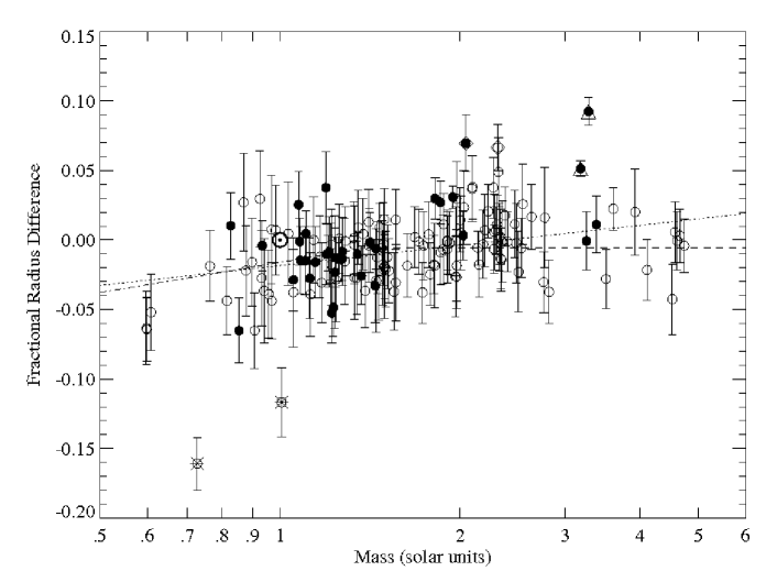
Figure 1: The relative radius discrepancy $\delta R_{*}$ for stars in the TAG sample, plotted against stellar mass $M_{*}$. The error bars show 1-$\sigma$ (assumed symmetrical) errors derived from the MCMC analysis, added in quadrature to the radius errors quoted by TAG. The stars for which there are individual estimates of $[Z]$ are shown as filled circles. I show the Sun’s position as a large $\sun$ symbol. the dotted line show the results of a fit to $\delta R_{*}$ as a linear function of $\log M_{*}$. The dashed line is a fit to the piecewise linear function of $\log M_{*}$ described in the text. Stars excluded from these fits are plotted with special symbols, and are described in the text.

deviation from those that were provided as input. The values of $M_{*}$, $R_{*}$, and $A_{*}$ derived by this method are listed in the last 3 columns (labeled “fit”) of Table 1, and in the corresponding columns of Table 2.

To compare input and output masses and radii, for each star I computed the normalized discrepancy $\delta M_{*}\ =(M_{output}-M_{input})/M_{input}$, and $\delta R_{*}=(R_{output}-R_{input})/R_{input}$. Figure 1 shows $\delta R_{*}$ plotted against the stellar masses estimated by TAG. Since the fits included a strong constraint on the stellar mean density, (as calculated from the provided values of $M_{*}$ and $R_{*}$) I obtained the nearly perfect equality $\delta M_{*}\ =\ 3\delta R_{*}$. One of the quantities $\delta M_{*}$ or $\delta R_{*}$ is therefore redundant, and can easily be computed from the other. In what follows, I will frame the discussion in terms of the discrepancy in radius $\delta R_{*}$.

From the Figure, it is evident that the $\rho_{*}$ method of estimating stellar radii works fairly well. Aside from a few outliers, the RMS deviation of $\delta R_{*}$ is 2.6%, while that of $\delta M_{*}$ (not plotted) is 3 times as large at 7.8%. The discrepancies are, however, predominantly negative, and they vary systematically with stellar mass. The sense of this trend is that the masses and radii derived using the $\rho_{*}$ method are generally too small, and in percentage terms, the more so for smaller stars. I have plotted discrepancies as a function of the stellar mass because this parameter is independent of stellar age. But since almost all of the stars on this plot are on the main-sequence or only slightly evolved, changing the independent variable to stellar radius or $T_{\rm eff}$ would show essentially the same picture. These parameters are so tightly correlated along this part of the main sequence that without further information, one can hardly say which of them (or what combination of them) is most central to the observed effect.

Fitting $\delta R_{*}$ to a linear function of $\log M_{*}$ yields

$$\delta R_{*}\ =\ (-0.0175\pm 0.0023)\ +\ (0.0561\pm 0.0076)\log M_{*}$$

This fit shows unambiguously that $\delta R_{*}$ is negative and has a trend with mass. The coefficients are nonzero with high statistical significance – more than 6$\sigma$ for each, with the fits removing about one-third of the variance in the data set, and shrinking the $\chi^{2}$ statistic by 40. Of course, one can also fit more complicated functions to the data. For instance, a piecewise linear function that has zero slope for $M_{*}\ \geq\ 1.4M_{\sun}$ fits the data marginally (but not compellingly) worse than does a single linear function; this is shown as dashed lines in the Figure. It is described by

$$\delta R_{*}\ =\ (0.0980\pm 0.020)\log(M_{*}/1.4),\ M_{*}<1.4$$

$$\delta R_{*}\ =\ (-0.0021\pm.098),\ M_{*}\geq 1.4$$

I excluded 6 outlying stars from the least-squares fits in Fig. 1. These are the two binaries V1174 Ori and OGLE 051019, as well as the primary components of SZ Cen and TZ For. All of these stars except perhaps SZ Cen are unusual as regards their evolutionary state or metallicity. Their individual peculiarities are described in section 4.4 below.

So far I have discussed only the masses and radii of stars in the TAG sample. Considering the best-fitting age values gives further evidence that the evolution models are failing for at least some stars. Stars with masses larger than 1 $M_{\sun}$ have, almost without exception, inferred ages that are less (usually much less) than that of the Milky Way. On the other hand, stars below solar mass have, with very few exceptions, inferred ages considerably greater than the Sun’s, and most often greater than a Hubble time. The record-holder in this regard is V1174 Ori B, with an apparent age that is greater than 100 GY, but many other low-mass stars display impossible ages.

The likely reason for these excessive age estimates is that the low-mass stars in the TAG sample have mean densities that are so low that stars with the observed values of $T_{\rm eff}$ and $[Z]$ attain them only after they are significantly evolved. Given the extended main-sequence lifetimes of these stars, such evolution can take a very long time. A related possibility is that, for low-mass stars, the measured effective temperatures are systematically too low. If this were the case, then the ZAMS model for a cool star would, in addition to being too cool, be smaller and more dense than it should be. Getting such a model to the observed $\rho_{*}$ would then require greater age than it should, and perhaps greater than possible. In either case, one can be sure that model-fitting solutions that require unphysical ages indicate something wrong with the models.

4 Discussion

Systematic differences between YY models and the samples of stars described in the previous section are concerning, even if they are rather small. But the way in which the differences are interpreted (and perhaps corrected) depends on how they arise. Three general sources of systematic error seem possible. First, the masses and radii estimated by the $\rho_{*}$ method may be incorrect because of systematic errors in the input data. Second, the chosen samples of stars may be systematically different from the galactic mean, or at least from those stars that one expects to encounter in planet searches. Last, the evolution models may simply be erroneous in some respects. Any or all of these possibilities may be true to some extent. I consider each of them below.

4.1 Systematic Errors in Input Data

Biased input data may of course lead to biased estimates of stellar mass and radius. In particular, values of $T_{\rm eff}$ and $[Z]$ derived from comparisons between observed spectra and stellar atmospheres models may not correspond exactly to $T_{\rm eff}$ and $[Z]$ as used in the stellar evolution models. Moreover, such inaccurate correspondence might plausibly depend on $T_{\rm eff}$ itself, which in principle could generate the observed lack of agreement. ($\rho_{*}$ might be in error also, but as applied to the TAG sample of EBs and to the seismically-constrained stars it is correct by definition, and as applied to transiting planets it depends only on such well-established physics that its reliability seems assured.)

Systematically inaccurate reddening estimates might also influence the masses and radii, by generating systematic errors in the observed $T_{\rm eff}$ values. This effect would however be strongest for the hottest and most luminous stars in the sample, since such stars tend to be the most reddened. There is no evidence in Fig. 1 for an effect of this sort, so I have not pursued this possibility.

To assess whether biased $T_{\rm eff}$ or $[Z]$ values might account for the observed discrepancy, I estimated the sensitivities $\partial\log R_{*}/\partial\log T_{\rm eff}$ and $\partial\log R_{*}/\partial[Z]$ by perturbing the input values for the TAG sample. Figure 2 shows these sensitivities as a function of $\log M_{*}$, computed using perturbations of 0.007 in $\log T_{\rm eff}$ and 0.1 dex in $[Z]$.

Figure 2: Sensitivities of the estimate of $R_{*}$ resulting from the $\rho_{*}$ method for stars in the TAG sample of eclipsing binaries. The sensitivity to $[Z]$ (upper panel) was computed using $\delta[Z]=0.1$; the sensitivity to $T_{\rm eff}$ (lower panel) used $\delta T_{\rm eff}=0.007$. Dashed lines show the results of robust fits to linear functions of $\log M_{*}$.

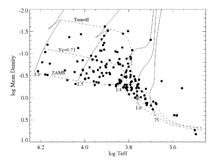
Figure 3: $\rho_{*}\ vs\ \log T_{\rm eff}$ plot for the stars in the TAG sample. Yonsei-Yale evolutionary tracks for stars with $M_{*}=$ {0.75, 1., 1.4, 2., 5.}$M_{\sun}$ are overplotted as solid lines. Loci of constant central $Y$ are plotted as dashed lines, corresponding to the ZAMS, $Y_{c}$(solar), and main-sequence turnoff. The Sun is indicated with a $\sun$ symbol.

Not all of the binaries yielded valid differences, because of jumps between multiple solutions as described in section 2. For the majority of stars, however, the results indicate that the sensitivities are only weakly mass-dependent. A robust straight-line fit to the sensitivities yields

$$\partial\log R_{*}/\partial\log T_{\rm eff}\ =\ 0.48\ -\ 0.12\log M_{*}\$$

$$\partial\log R_{*}/\partial[Z]\ =\ 0.048\ -\ 0.029\log M_{*}\ .$$

Both of these sensitivities are well defined for $\log M_{*}\geq 0.15$, and less so for smaller masses. Even at 1 solar mass, however, it seems safe to estimate that to cause the observed -1.7% discrepancy in $\delta R_{*}$ would require systematic errors of about 200 K at $T_{\rm eff}=5800$ K, or more than 0.15 dex in $[Z]$. Systematic errors of this size are essentially impossible for $T_{\rm eff}$, and implausible for $[Z]$. Thus, while one cannot altogether discount systematic errors in these observed parameters as contributing to the discrepancy between TAG parameters and those from the $\rho_{*}$ analysis, it seems unlikely that they make an important contribution.

4.2 Bias in the TAG Sample

Perhaps the most striking point to be made from Fig. 1 is that the Sun, to which the YY models are calibrated, is not closely representative of the stars of its general type in this sample. Compared to its neighbors in Fig. 1, it is assigned a larger mass and radius than is typical, by about 5% and 1.6%, respectively. These discrepancies clearly do not arise from errors in the Sun’s properties. There seem to be three possibilities: the EB stars that fall near the Sun in mass and radius are subject to systematic errors of a few percent in their mass and radius measurements, or they are subject to selection bias of similar magnitude, or there is genuine star-to-star variability in the stellar mass-radius-luminosity relationship. Again, none of these possibilities excludes the others; all may be acting to some degree.

To address these issues it is helpful to display the data in a way that separates the observational data (EB masses and radii) from issues of evolution modeling and data fitting. Figure 3 shows $\rho_{*}$ plotted against $\log T_{\rm eff}$ for the TAG sample of stars, and for the Sun. The axes are oriented as in a color-temperature diagram, with temperature increasing to the left, and $\rho_{*}^{-1}$ (a proxy for luminosity) increasing upwards. Overlaid are (solid lines) YY evolution tracks for a sampling of stellar masses, and (dashed lines) loci corresponding to the zero-age main sequence (ZAMS), main-sequence middle age (with about 71% helium in the core, corresponding to the Sun’s evolutionary state), and the age of turnoff from the main sequence. Even more than in Fig. 1, the Sun lies at or near one boundary of the region populated by stars: it has $\rho_{*}$ as large or larger than all other stars with similar $T_{\rm eff}$. Evolution in stars of roughly solar mass carries them upward on this diagram, to lower $\rho_{*}$ and higher luminosity. So, barring a statistical fluke, it seems either that all of the low-mass stars in the TAG sample are at least as evolved as the Sun, or that evolution models that accurately describes the Sun do not describe the average properties of the TAG sample.

Two obvious sources of bias in the TAG sample are Malmquist bias, which will favor detection of more luminous binaries, and a geometrical bias towards stars with larger radii, since (assuming random orbital inclinations) these are more likely to present themselves as EBs. These effects are however inadequate to account for the strength or the morphology of the observed bias. According to the YY evolution tracks, the present-day Sun is about 36% more luminous and 12% larger in radius than it was on the ZAMS. Its detectability as the larger member of an EB should be proportional to the volume within which it is brighter than some limiting apparent magnitude, multiplied by the ratio of solid angles within which the rotation axis must lie in order for eclipses to occur. The first factor is at most proportional to $L_{*}^{3/2}$, while for well-detached EBs such as found in the TAG sample, the second factor is proportional to $R_{*}$. Sun-like stars in the second half of their main-sequence lifetime thus should be over-represented among the TAG stars by a factor of at most about 1.8, relative to younger stars of similar mass. It is surprising to find the latter group totally absent. Moreover, the factors favoring detection of somewhat evolved stars should be similar for stars of all masses, whereas the trend seen in Fig. 3 is quite different. For stars with masses greater than 1.4 $M_{\sun}$, the ZAMS is coincident with the observed maximum-$\rho_{*}$ boundary, and for more massive stars there are roughly equal numbers in the first and last halves of their main-sequence lifetimes. But for masses below 0.8 $M_{\sun}$, no stars are found anywhere within the YY main sequence (although the significance of this observation is shaky because of the small number of TAG stars in this mass range). On balance, it seems unlikely that Malmquist and geometrical selection bias by themselves provide an adequate explanation for the paucity of high-$\rho_{*}$ Sun-like stars in the TAG sample.

Since most of the TAG stars lack metallicity determinations, another possible bias is that the true $[Z]$ values for these stars differs systematically from the assumed Gaussian distribution with $[Z]=0.0\pm 0.2$. To test this idea I performed fits to the observed $\delta R$ vs. $\log M_{*}$ dependence, using only the 32 stars with measured metallicities. For both the linear and piecewise linear fits, the coefficients of the mass-dependent part of the variation agreed with those in Eqs. (1-2) within 1$\sigma$, and for both fits these coefficients differed from zero by about 2.5$\sigma$. Thus, the subset of stars with measured metallicities gives results that are consistent with those from the full sample, but with worse precision.

To explore a possible $[Z]$ bias further, I artificially altered the model $[Z]$ values as a linear function of $\log T_{\rm eff}$, in order to remove the mass dependence seen in Fig 1. For all but the least massive ($M\leq 0.6M_{\sun}$) stars, I achieved this by increasing $[Z]$ by an amount $\delta[Z]=+0.1-2\log(T_{\rm eff}/T_{\sun})$, but only for $T_{\rm eff}\leq 6400$K. This implies that to produce the observed radii, the $\simeq$70 low-mass stars in the TAG sample would need to be systematically metal-rich compared to the Sun; about 25% would require $[Z]\geq 0.2$, and about 10% would need $[Z]\geq 0.4$. While such a distribution of $[Z]$ is conceivable, it is implausible a priori. A survey of about 12,000 bright stars in the solar neighborhood (Nordström et al., 2004) shows a distribution that is centered at $[Z]\simeq-0.17$, with a characteristic width of about 0.22 dex. Significantly metal-rich stars are therefore fairly rare; only 4% of Nordström’s sample show $[Z]\geq 0.2$, and fewer than 0.4% have $[Z]\geq 0.4$. Since no obvious metallicity selection is operating in the choice of EBs in the TAG sample, it is implausible that the sample should be as skewed towards high $[Z]$ as is required to explain Fig. 1. On the other hand, systematically high $[Z]$ would help reduce the large ages attributed to many low-mass stars, because increasing metallicity tends to decrease stellar mean density at constant $T_{\rm eff}$ and age. A final curiosity is that the very lowest-mass stars (smaller than about 0.6 $M_{\sun}$) show radius changes with $[Z]$ that are smaller than (and sometimes opposite in sign to) those of their more massive brethren. Evidently it is dangerous to draw conclusions base on these stars, presumably because there are many changes in important physical processes as one nears the boundary between K and M stars.

A bias that is more likely to be important relates to the stars’ angular momenta and magnetic activity. Torres et al. (2006), López-Morales (2007), and Morales et al. (2008) have noted that some rapidly-rotating, magnetically-active EB component stars have temperatures that are lower and radii that are larger than expected for their masses or luminosities. Conspicuous examples of such stars include V1061 Cyg (Torres et al., 2006), and CV Boo (Torres et al., 2009). Both models (Chabrier et al., 2007; Clausen et al., 2009) and general structural considerations suggest that magnetic processes in stellar outer convection zones are responsible for inflating stars in this way. Moreover, as pointed out by TAG and others, EB systems are strongly selected for small, short-period orbits. As a result, their components usually are tidally locked, and rotate rapidly compared to all but the youngest field stars. Thus, one expects the TAG sample to be biased in the sense that its members have larger radii and smaller $T_{\rm eff}$ than would a similar sample of single stars. The paucity of high-density of stars seen in Fig. 3 is consistent with this expectation. The lack of dense stars is most evident for sub-solar masses (for which stars have deep convection zones), and weak or absent for stars above 1.4 $M_{\sun}$, for which surface convection zones almost vanish.

4.3 Asteroseismic Sample

The 15 stars with properties listed in Table 2 have measurements of their pulsation frequencies that constrain their large frequency separations $\Delta\nu$, and hence the values of $\rho_{*}$ (e.g., Hansen et al. (2004)). When combined with other astronomical data (the details vary from star to star), this information allows accurate estimates of $R_{*}$ and $M_{*}$. In most cases, the stellar oscillations have been observed in the radial velocity signal; for this to be feasible, the stars must have small values of the rotational line broadening $v\sin i$. Hence, these stars should not suffer from the rotation/activity bias ascribed to the TAG sample. Two stars, $\alpha$ Cen A and B, appear in both the TAG and the asteroseismic lists.

Fig. 4 shows the result of applying the $\rho_{*}$ method to the asteroseismic sample of stars and plotting mass and radius discrepancies as in Fig. 1. Expressed in the same terms as Eqns (1) and (2), a fit to these data yields

$$\delta R_{*}\ =\ (0.0013\pm 0.0068)\ -\ (0.002\pm 0.046)\log M_{*}$$

and

$$\delta R_{*}\ =\ (0.042\pm 0.075)\log(M_{*}/1.4),\ M_{*}<1.4$$

$$\delta R_{*}\ =\ (0.005\pm.009),\ M_{*}\geq 1.4$$

Evidently the YY models fits the asteroseismology sample within the errors. Moreover, the zero points of the linear fits to the TAG and asteroseismology samples disagree by 2.5 $\sigma$, so there is moderately strong evidence that the two distributions are indeed drawn from different populations. The fits also yield discrepant slopes for the two samples, but the asteroseismology sample slope is so poorly constrained that the difference between slopes is only about 1 $\sigma$.

Figure 5 shows the $\rho_{*}$ vs $T_{\rm eff}$ plot for the asteroseismic sample. One star, $\zeta$ Hyi, is a true giant with $\log\rho_{*}=-2.6$, and hence falls outside the plotted range of the figure. There are 4 stars out of 15 in the asteroseismology group that have equal or greater density and equal or younger evolutionary age than the Sun. This is consistent with the hypothesis that low-mass EB component stars have systematically lower density than do slowly-rotating field stars of the same $T_{\rm eff}$. As yet, however, the number of stars with asteroseismic mass and radius measurements is too small to justify a firm conclusion in this regard. Moreover, as noted earlier, asteroseismic parameter estimation has its own model dependencies. Agreement between asteroseismic and $\rho_{*}$ methods for estimating parameters may say more about similarities between the models used than it says about the accuracy of either set of models in representing real stars.

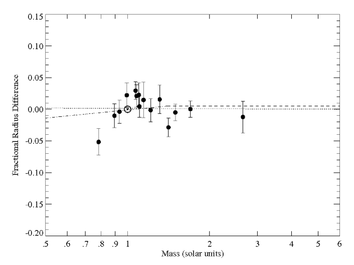
Figure 4: Same as Fig. 1, but for stars with asteroseismic estimates of $\rho_{*}$.

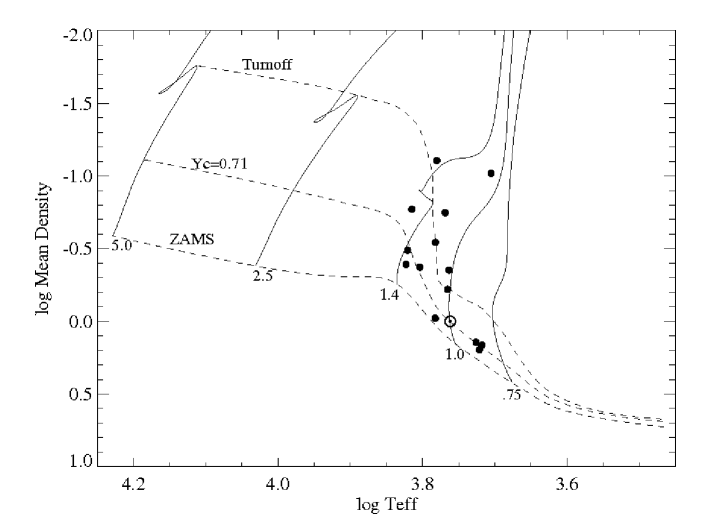
Figure 5: Same as Fig. 3, but for the sample of stars with asteroseismic estimates of $M_{*}$ and $R_{*}$.

4.4 Stars with Unusual Properties

In Figures 1 and 4, a few stars stand out as being significantly inconsistent with the mean relation between $\delta R_{*}$ and $M_{*}$. I did not include these stars in the least-squares fits described in section 3, so it is worthwhile to understand in what other ways they differ from the norm. In most cases there is a ready explanation for their odd radii.

The two stars overplotted with asterisks in Fig. 2 have fractional radius differences smaller than -0.1. They are the components of VB1174 Ori, a pre-main-sequence system (Stassun et al., 2004) with oversize components that are still contracting.

The two stars overplotted with triangles are components of OGLE-05019.64-685812.3 (Pietrzyński et al., 2009). This member of the Large Magellanic Cloud is the faintest and the second most metal-deficient system in the TAG list of binaries (after V432 Aur). Its assigned metallicity ($[Z]=-0.5$) has not been measured directly; rather it is inferred from the mean metallicity of its population. Its small radius relative to the YY models might therefore result if its metallicity were actually about $[Z]=-1.1$, or as a result of errors in the models themselves, or in how the latter are used. The last explanation seems most likely, as these stars may in fact be clump giants, which lie beyond the oldest evolutionary stage tabulated in the YY models.

The 2 stars with $\delta R_{*}\simeq+0.05$ and overplotted with diamonds are the primary components of SZ Cen (with $M_{*}=2.31$) and TZ For ($M_{*}=2.05$). The SZ Cen system is poorly represented by evolution tracks for coeval stars with equal initial composition (Gronbech et al., 1977), but the reason for this failure is obscure. TZ For consists of a pair of giants, with the primary component’s radius being more than 8 $R_{\sun}$ (Andersen et al., 1991). These authors found that the more luminous, cooler component of this system (identified as TZ For A in the compilation by TAG, but as TZ For B in Andersen et al. (1991)) can be reconciled with the properties its companion only if the former is in the core helium burning stage of evolution. Since the YY models extend only to the tip of the giant branch, this star cannot be represented by them.

Finally, the lowest-mass and most discrepant star in the list of stars with asteroseismic data is $\tau$ Cet (Teixeira et al., 2009). This star is well known for having extremely low magnetic activity, yet its asteroseismic radius appears 5% larger than the YY models would indicate given its $T_{\rm eff}$ and $[Z]$, even if one allows the unreasonable age of 24 GY. In this case the asteroseismic data were compromised by instrumental noise, and hence may be open to question. Rather than speculate about causes, it seems best in this instance to wait for further observations.

4.5 Conclusions

The original motivation for this paper was to assess the accuracy of the $\rho_{*}$ method for estimating radii of the host stars of transiting extrasolar planets. Since the reliability of the method is almost entirely dependent upon the reliability of stellar evolution models, this question can also be framed in terms of the ability of such models (in the present case, the Yonsei-Yale models) to represent the true mass-radius-luminosity dependencies of real stars. The short answer to the initial question is yes, without any corrections or adjustments the $\rho_{*}$ method implemented with the YY evolution tracks will yield stellar radii that are accurate within (at worst) about 5%, for a large majority of stars. This accuracy in radius is already good enough to support useful measurements of planetary density from transit measurements by Kepler and other spaceborne photometry missions (Seager et al., 2007), although the corresponding 15% uncertainty in mass may be problematic. However, if one confines attention to the asteroseismic sample of single, slowly-rotating stars (Table 2), the accuracy of $\rho_{*}$-based radius estimates appears considerably better, perhaps as good as 2% RMS. At this level, the accuracy of radius estimates is limited by probable systematic errors not only in the evolution models, but to a similar degree by errors in estimates of stellar $T_{\rm eff}$ and $[Z]$. Improving this situation will require further work to obtain accurate spectroscopic estimates of these quantities and to understand the correlated errors between them, especially for spectra with lines that are significantly broadened by stellar rotation.

Although the $\rho_{*}$ method (with YY models) works well on average, it shows mass-dependent systematic errors of several percent when applied to components of eclipsing binary systems. The sense of these errors is that observed EB component radii and masses are larger than those predicted by the YY models; these differences are largest for low-mass stars. A plausible reading of the data (but one that is not compelled by statistics) is that the radius differences are zero for stars with more than about 1.4 solar masses, corresponding to the mass at which surface convection zones shrink to a negligible fraction of the stellar radius. For many years, it has been noted that rapidly-rotating, magnetically-active stars may have radii that are up to 10% larger than their masses and luminosities would imply (Hoxie, 1973; Lacy, 1977; Popper, 1997). These claims are based for the most part on results for unequal-mass EB components, for which it proves impossible to fit masses, radii, and luminosities if the components are assumed to be coeval and to have the same composition. Examples of such stars include CV Boo B (Torres et al., 2009) and V1061 Cyg B (Torres et al., 2006). Theory (Chabrier et al., 2007) suggests that the radius expansion results from blockage of the convective energy flux by strong magnetic fields in the stellar convection zones. The mass dependence of EB radius discrepancies seen in Fig. 1 is thus likely to be the population-averaged expression of the same physical process.

It is possible that the stellar models calculated by Baraffe (Chabrier & Baraffe, 1997) fit the observed properties of cool, low-mass stars better than the YY models do. These models are intended to treat such stars, using non-gray atmospheres and smaller mixing-length parameters that act to reduce the efficiency of energy transport in the outer stellar layers. It would be worthwhile (but is outside the scope of this paper) to perform a detailed comparison of the TAG masses and radii with those inferred using the $\rho_{*}$ method and the Baraffe models.

Stars with asteroseismic estimates of $\rho_{*}$ do not show the radius discrepancies found in the TAG sample. This sample of stars are all magnetically inactive, slow rotators. The good agreement between their observed radii and those predicted by the YY models argues in favor of magnetic activity having a visible influence on the radii of low-mass stars. The number of asteroseismically-measured stars is, however, as yet too small to allow a firm conclusion that these stars are drawn from a different population than the eclipsing binaries. Future work will surely improve this situation, especially insofar as spaceborne photometry allows asteroseismic measurements on rapidly-rotating stars, which are difficult to measure with Doppler methods.

Table 1: Eclipsing Binary Stars with Accurate Mass and Radius Estimates.

Star	$M_{*}$	$M_{*}$	$R_{*}$	$R_{*}$	$T_{\rm eff}$	$T_{\rm eff}$	$[Z]$	$[Z]$	$M_{fit}$	$R_{fit}$	Agefit
	$(M_{\sun}$)	RMS	($R_{\sun}$)	RMS	(K)	RMS		RMS	($M_{\sun}$)	($R_{\sun}$)	(GY)
U Oph B	4.739	0.072	3.111	0.034	15590	250	0.000	0.200	4.711	3.104	0.05
DI Her B	4.524	0.066	2.478	0.046	15100	700	0.000	0.200	4.141	2.406	0.01
V760 Sco B	4.609	0.073	2.642	0.066	16300	500	0.000	0.200	4.757	2.670	0.01
MU Cas A	4.657	0.095	4.196	0.058	14750	800	0.000	0.200	4.912	4.271	0.08
MU Cas B	4.575	0.088	3.671	0.057	15100	800	0.000	0.200	4.809	3.732	0.07
GG Lup A	4.106	0.044	2.381	0.025	14750	450	0.000	0.200	4.001	2.361	0.01
GG Lup B	2.504	0.023	1.726	0.019	11000	600	0.000	0.200	2.414	1.707	0.04
$\zeta$ Phe A	3.921	0.045	2.853	0.015	14400	800	0.000	0.200	4.186	2.915	0.06
$\zeta$ Phe B	2.545	0.026	1.854	0.011	12000	600	0.000	0.200	2.867	1.930	0.03
$\chi$2 Hya A	3.605	0.078	4.391	0.039	11750	190	0.000	0.200	3.860	4.492	0.17
$\chi$2 Hya B	2.632	0.049	2.160	0.030	11100	230	0.000	0.200	2.780	2.199	0.14
IQ Per A	3.504	0.054	2.446	0.024	12300	230	0.000	0.200	3.226	2.379	0.09
IQ Per B	1.730	0.025	1.499	0.016	7700	140	0.000	0.200	1.597	1.460	0.14
V906 Sco A	3.378	0.071	4.521	0.035	10400	500	0.140	0.060	3.490	4.570	0.23
V906 Sco B	3.253	0.069	3.515	0.039	10700	500	0.140	0.060	3.228	3.506	0.24
OGLE 051019 A	3.278	0.032	26.060	0.290	5300	100	-0.500	0.100	4.322	28.577	0.13
OGLE 051019 B	3.179	0.029	19.770	0.340	5450	100	-0.500	0.100	3.727	20.846	0.19
PV Cas A	2.816	0.050	2.301	0.020	10200	250	0.000	0.200	2.529	2.219	0.25
PV Cas B	2.757	0.054	2.258	0.019	10190	250	0.000	0.200	2.514	2.189	0.24
V451 Oph A	2.769	0.062	2.642	0.031	10800	800	0.000	0.200	2.889	2.679	0.24
V451 Oph B	2.351	0.052	2.029	0.028	9800	500	0.000	0.200	2.347	2.027	0.24
WX Cep A	2.533	0.050	3.997	0.030	8150	250	0.000	0.200	2.525	3.993	0.57
WX Cep B	2.324	0.045	2.712	0.023	8900	250	0.000	0.200	2.342	2.719	0.53
TZ Men A	2.482	0.025	2.017	0.020	10400	500	0.000	0.200	2.515	2.025	0.16
TZ Men B	1.500	0.010	1.433	0.014	7200	300	0.000	0.200	1.494	1.431	0.18
V1031 Ori A	2.468	0.018	4.324	0.034	7850	500	0.000	0.200	2.540	4.365	0.59
V1031 Ori B	2.281	0.016	2.979	0.064	8400	500	0.000	0.200	2.293	2.984	0.64
V396 Cas A	2.397	0.025	2.593	0.014	9225	150	0.000	0.200	2.388	2.589	0.46
V396 Cas B	1.901	0.019	1.780	0.010	8550	120	0.000	0.200	1.925	1.787	0.39
$\beta$ Aur A	2.375	0.027	2.766	0.018	9350	200	0.000	0.200	2.500	2.814	0.44
$\beta$ Aur B	2.304	0.030	2.572	0.018	9200	200	0.000	0.200	2.386	2.602	0.47
GG Ori A	2.342	0.016	1.854	0.025	9950	200	0.000	0.200	2.311	1.845	0.13
GG Ori B	2.338	0.016	1.832	0.025	9950	200	0.000	0.200	2.300	1.822	0.12
V364 Lac A	2.333	0.015	3.310	0.021	8250	150	0.000	0.200	2.355	3.320	0.64
V364 Lac B	2.295	0.024	2.986	0.020	8500	150	0.000	0.200	2.323	2.998	0.61
YZ Cas A	2.317	0.020	2.539	0.026	10200	300	0.000	0.200	2.697	2.671	0.31
YZ Cas B	1.352	0.009	1.351	0.014	7200	300	0.000	0.200	1.449	1.385	0.18
SZ Cen A	2.311	0.026	4.557	0.032	8100	300	0.000	0.200	2.785	4.849	0.47
SZ Cen B	2.272	0.021	3.626	0.026	8380	300	0.000	0.200	2.525	3.755	0.55
V624 Her A	2.277	0.014	3.032	0.051	8150	150	0.000	0.200	2.228	3.010	0.71
V624 Her B	1.876	0.013	2.211	0.034	7950	150	0.000	0.200	1.923	2.229	0.83
V885 Cyg A	2.228	0.026	3.388	0.026	8150	150	0.000	0.200	2.368	3.457	0.64
V885 Cyg B	2.000	0.029	2.346	0.017	8375	150	0.000	0.200	2.083	2.378	0.68
GZ CMa A	2.199	0.017	2.494	0.031	8800	350	0.000	0.200	2.241	2.509	0.56
GZ CMa B	2.006	0.012	2.133	0.037	8500	350	0.000	0.200	2.035	2.143	0.60
V1647 Sgr A	2.184	0.037	1.832	0.018	9600	300	0.000	0.200	2.220	1.842	0.18
V1647 Sgr B	1.967	0.033	1.668	0.017	9100	300	0.000	0.200	2.026	1.684	0.14
EE Peg A	2.151	0.024	2.090	0.025	8700	200	0.000	0.200	2.064	2.061	0.51
EE Peg B	1.332	0.011	1.312	0.013	6450	300	0.000	0.200	1.340	1.314	0.46
AI Hya A	2.140	0.038	3.917	0.031	6700	60	0.000	0.200	2.072	3.875	1.06
AI Hya B	1.973	0.036	2.768	0.019	7100	65	0.000	0.200	1.854	2.711	1.21
VV Pyx A	2.097	0.022	2.169	0.020	9500	200	0.000	0.200	2.347	2.251	0.37
VV Pyx B	2.095	0.019	2.169	0.020	9500	200	0.000	0.200	2.347	2.252	0.37
TZ For A	2.045	0.055	8.330	0.120	5000	100	0.100	0.150	2.489	8.893	0.66
TZ For B	1.945	0.027	3.966	0.088	6350	100	0.100	0.150	2.135	4.087	1.05
V459 Cas A	2.030	0.036	2.014	0.020	9140	300	0.000	0.200	2.175	2.061	0.39
V459 Cas B	1.973	0.034	1.970	0.020	9100	300	0.000	0.200	2.153	2.028	0.39
EK Cep A	2.025	0.023	1.580	0.007	9000	200	0.070	0.050	1.928	1.583	0.08
EK Cep B	1.122	0.012	1.316	0.006	5700	200	0.070	0.050	1.042	1.283	7.71
KW Hya A	1.973	0.036	2.127	0.016	8000	200	0.000	0.200	1.893	2.098	0.78
KW Hya B	1.485	0.017	1.480	0.013	6900	200	0.000	0.200	1.450	1.468	0.60
WW Aur A	1.964	0.010	1.929	0.011	7960	420	0.000	0.200	1.813	1.878	0.69
WW Aur B	1.814	0.008	1.838	0.011	7670	410	0.000	0.200	1.714	1.803	0.79
WW Cam A	1.920	0.013	1.912	0.016	8350	135	0.000	0.200	1.917	1.911	0.56
WW Cam B	1.873	0.018	1.809	0.016	8240	135	0.000	0.200	1.852	1.802	0.52
V392 Car A	1.904	0.013	1.625	0.022	8850	200	0.000	0.200	1.945	1.636	0.14
V392 Car B	1.855	0.020	1.601	0.022	8630	200	0.000	0.200	1.884	1.609	0.14
AY Cam A	1.901	0.040	2.771	0.020	7250	100	0.000	0.200	1.914	2.777	1.11
AY Cam B	1.706	0.036	2.025	0.017	7395	100	0.000	0.200	1.715	2.028	1.10
RS Cha A	1.854	0.016	2.139	0.055	8050	200	0.170	0.010	2.010	2.197	0.63
RS Cha B	1.817	0.018	2.340	0.055	7700	200	0.170	0.010	1.986	2.410	0.81
MY Cyg A	1.806	0.025	2.243	0.050	7050	200	0.000	0.200	1.683	2.191	1.36
MY Cyg B	1.782	0.030	2.178	0.050	7000	200	0.000	0.200	1.648	2.122	1.42
EI Cep A	1.772	0.007	2.898	0.048	6750	100	0.000	0.200	1.828	2.928	1.36
EI Cep B	1.680	0.006	2.331	0.044	6950	100	0.000	0.200	1.703	2.341	1.42
BP Vul A	1.737	0.015	1.853	0.014	7715	150	0.000	0.200	1.738	1.853	0.81
BP Vul B	1.408	0.009	1.490	0.013	6810	150	0.000	0.200	1.423	1.495	1.00
FS Mon A	1.632	0.010	2.052	0.012	6715	100	0.000	0.200	1.539	2.012	1.82
FS Mon B	1.462	0.009	1.630	0.010	6550	100	0.000	0.200	1.348	1.586	2.28
PV Pup A	1.561	0.011	1.544	0.016	6920	300	0.000	0.200	1.449	1.506	0.86
PV Pup B	1.550	0.013	1.500	0.016	6930	300	0.000	0.200	1.468	1.472	0.50
V442 Cyg A	1.560	0.024	2.074	0.034	6900	100	0.000	0.200	1.615	2.098	1.53
V442 Cyg B	1.407	0.023	1.663	0.033	6800	100	0.000	0.200	1.467	1.686	1.52
EY Cep A	1.520	0.012	1.464	0.011	7090	150	0.000	0.200	1.494	1.455	0.25
EY Cep B	1.496	0.016	1.471	0.011	6970	150	0.000	0.200	1.470	1.462	0.42
HD 71636 A	1.511	0.007	1.570	0.026	6950	140	0.000	0.200	1.467	1.555	0.98
HD 71636 B	1.285	0.006	1.362	0.026	6440	140	0.000	0.200	1.283	1.361	1.83
RZ Cha A	1.493	0.022	2.257	0.016	6450	150	0.000	0.200	1.556	2.288	2.11
RZ Cha B	1.493	0.022	2.257	0.016	6450	150	0.000	0.200	1.399	2.209	3.03
GX Gem A	1.488	0.011	2.327	0.012	6195	100	0.000	0.200	1.446	2.305	3.09
GX Gem B	1.467	0.010	2.236	0.012	6165	100	0.000	0.200	1.484	2.245	2.69
BW Aqr A	1.479	0.019	2.063	0.044	6350	100	0.000	0.200	1.463	2.056	2.50
BW Aqr B	1.377	0.021	1.786	0.043	6450	100	0.000	0.200	1.411	1.801	2.41
DM Vir A	1.454	0.008	1.765	0.017	6500	100	0.000	0.200	1.402	1.744	2.31
DM Vir B	1.448	0.008	1.765	0.017	6500	300	0.000	0.200	1.424	1.755	2.12
V570 Per A	1.447	0.009	1.521	0.034	6842	50	0.020	0.030	1.423	1.512	1.10
V570 Per B	1.347	0.008	1.386	0.019	6562	50	0.020	0.030	1.308	1.372	1.48
CD Tau A	1.442	0.016	1.798	0.015	6200	50	0.080	0.150	1.358	1.762	3.11
CD Tau B	1.368	0.016	1.585	0.018	6200	50	0.080	0.150	1.289	1.554	3.23
AD Boo A	1.414	0.009	1.614	0.014	6575	120	0.100	0.150	1.418	1.615	1.75
AD Boo B	1.209	0.006	1.217	0.010	6145	120	0.100	0.150	1.200	1.214	1.97
V1143 Cyg A	1.388	0.016	1.347	0.023	6450	100	0.000	0.200	1.269	1.307	1.50
V1143 Cyg B	1.344	0.013	1.324	0.023	6400	100	0.000	0.200	1.257	1.295	1.60
IT Cas A	1.332	0.009	1.595	0.018	6470	100	0.000	0.200	1.349	1.601	2.42
IT Cas B	1.329	0.008	1.563	0.018	6470	100	0.000	0.200	1.333	1.564	2.43
V1061 Cyg A	1.282	0.015	1.616	0.017	6180	100	0.000	0.200	1.287	1.618	3.46
V1061 Cyg B	0.932	0.007	0.967	0.011	5300	150	0.000	0.200	0.809	0.923	16.36
VZ Hya A	1.271	0.009	1.314	0.005	6645	150	-0.200	0.120	1.258	1.309	1.41
VZ Hya B	1.146	0.006	1.113	0.007	6290	150	-0.200	0.120	1.124	1.105	1.51
V505 Per A	1.269	0.007	1.287	0.024	6510	50	-0.120	0.030	1.222	1.270	1.71
V505 Per B	1.251	0.007	1.266	0.024	6460	50	-0.120	0.030	1.201	1.249	1.87
HS Hya A	1.255	0.008	1.276	0.007	6500	50	0.000	0.200	1.297	1.289	0.87
HS Hya B	1.219	0.007	1.217	0.007	6400	50	0.000	0.200	1.259	1.229	0.78
RT And A	1.240	0.030	1.256	0.015	6100	150	0.000	0.200	1.154	1.226	3.07
RT And B	0.907	0.017	0.907	0.011	4880	100	0.000	0.200	0.727	0.840	25.68
UX Men A	1.235	0.006	1.348	0.013	6200	100	0.040	0.100	1.205	1.337	3.05
UX Men B	1.196	0.007	1.275	0.013	6150	100	0.040	0.100	1.173	1.267	3.05
AI Phe A	1.234	0.004	2.932	0.048	5010	120	-0.140	0.100	1.292	2.978	4.24
AI Phe B	1.193	0.004	1.818	0.024	6310	150	-0.140	0.100	1.360	1.899	2.92
WZ Oph A	1.227	0.007	1.402	0.012	6165	100	-0.270	0.070	1.045	1.331	5.98
WZ Oph B	1.220	0.006	1.420	0.012	6115	100	-0.270	0.070	1.044	1.347	6.17
FL Lyr A	1.218	0.016	1.283	0.028	6150	100	0.000	0.200	1.173	1.267	3.05
FL Lyr B	0.958	0.012	0.962	0.028	5300	100	0.000	0.200	0.815	0.913	15.25
V432 Aur A	1.204	0.006	2.430	0.023	6080	85	-0.600	0.050	1.168	2.405	4.36
V432 Aur B	1.079	0.005	1.224	0.007	6685	85	-0.600	0.050	1.071	1.220	3.55
EW Ori A	1.174	0.012	1.134	0.011	5970	100	0.000	0.200	1.074	1.100	3.67
EW Ori B	1.124	0.009	1.083	0.011	5780	100	0.000	0.200	0.989	1.038	6.03
BH Vir A	1.166	0.008	1.247	0.024	6100	100	0.000	0.200	1.162	1.246	3.12
BH Vir B	1.052	0.006	1.135	0.023	5500	200	0.000	0.200	0.929	1.086	11.04
ZZ UMa A	1.139	0.005	1.514	0.019	5960	70	0.000	0.200	1.148	1.516	5.54
ZZ UMa B	0.969	0.005	1.156	0.010	5270	90	0.000	0.200	0.846	1.103	18.47
$\alpha$ Cen A	1.105	0.007	1.224	0.003	5824	26	0.240	0.040	1.124	1.231	4.69
$\alpha$ Cen B	0.934	0.006	0.863	0.005	5223	62	0.240	0.040	0.926	0.859	3.79
NGC188 KR V12 A	1.103	0.007	1.426	0.019	5900	100	-0.100	0.090	1.043	1.401	7.57
NGC188 KR V12 B	1.081	0.007	1.374	0.019	5875	100	-0.100	0.090	1.052	1.358	7.03
V568 Lyr A	1.074	0.008	1.400	0.016	5665	100	0.400	0.100	1.200	1.452	4.91
V568 Lyr B	0.827	0.004	0.768	0.006	4900	100	0.400	0.100	0.861	0.779	3.04
V636 Cen A	1.052	0.005	1.019	0.004	5900	85	-0.200	0.080	0.958	0.988	5.42
V636 Cen B	0.854	0.003	0.830	0.004	5000	100	-0.200	0.080	0.681	0.771	25.55
CV Boo A	1.032	0.013	1.263	0.023	5760	150	0.000	0.200	1.029	1.262	7.91
CV Boo B	0.968	0.012	1.174	0.023	5670	150	0.000	0.200	0.925	1.160	11.80
V1174 Ori A	1.006	0.013	1.338	0.011	4470	120	0.000	0.200	0.698	1.184	42.39
V1174 Ori B	0.727	0.010	1.063	0.011	3615	100	0.000	0.200	0.428	0.891	108.00
UV Psc A	0.983	0.008	1.110	0.023	5780	100	0.000	0.200	0.981	1.108	7.79
UV Psc B	0.764	0.004	0.835	0.018	4750	80	0.000	0.200	0.710	0.813	28.42
CG Cyg A	0.941	0.014	0.893	0.012	5260	180	0.000	0.200	0.834	0.858	11.18
CG Cyg B	0.815	0.013	0.838	0.011	4720	60	0.000	0.200	0.700	0.795	29.00
RW Lac A	0.926	0.006	1.187	0.004	5760	100	0.000	0.200	0.973	1.210	9.63
RW Lac B	0.869	0.004	0.964	0.004	5560	150	0.000	0.200	0.905	0.977	9.64
HS Aur A	0.898	0.019	1.005	0.024	5350	75	0.000	0.200	0.834	0.980	15.82
HS Aur B	0.877	0.017	0.874	0.024	5200	75	0.000	0.200	0.813	0.852	13.09
GU Boo A	0.609	0.006	0.627	0.016	3920	130	0.000	0.200	0.514	0.592	56.22
GU Boo B	0.598	0.006	0.623	0.016	3810	130	0.000	0.200	0.493	0.584	61.11
YY Gem A	0.599	0.005	0.619	0.006	3820	100	0.000	0.200	0.498	0.581	57.80
YY Gem B	0.599	0.005	0.619	0.006	3820	100	0.000	0.200	0.498	0.581	57.81
CU Cnc A	0.435	0.001	0.432	0.005	3160	150	0.000	0.200	0.425	0.434	1.40

Table 2: Stars with $M_{*}$ and $R_{*}$ estimates based on asteroseismology.

Star	$M_{*}$	$M_{*}$	$R_{*}$	$R_{*}$	$T_{\rm eff}$	$T_{\rm eff}$	$[Z]$	$[Z]$	$M_{fit}$	$R_{fit}$	Agefit	Source
	$(M_{\sun}$)	RMS	($R_{\sun}$)	RMS	(K)	RMS		RMS	($M_{\sun}$)	($R_{\sun}$)	(GY)
HD49933	1.079	0.073	1.385	0.031	6650	75	-0.440	0.060	1.150	1.414	3.47	Bruntt (2009)
HD175726	0.993	0.060	1.014	0.035	6060	50	-0.100	0.060	1.063	1.037	2.34	Bruntt (2009)
HD181420	1.311	0.063	1.595	0.032	6620	100	0.000	0.120	1.391	1.627	1.96	Bruntt (2009)
HD181906	1.144	0.119	1.392	0.054	6365	120	-0.110	0.140	1.224	1.423	3.10	Bruntt (2009)
70 Oph A	0.895	0.005	0.863	0.002	5322	40	0.011	0.050	0.870	0.855	7.56	Tang et al. (2008)
$\alpha$ Cen A	1.105	0.007	1.224	0.003	5824	26	0.240	0.040	1.124	1.231	4.69	Torres et al. (2009)
$\alpha$ Cen B	0.934	0.006	0.863	0.005	5223	62	0.240	0.040	0.926	0.859	3.79	Torres et al. (2009)
$\mu$ Ara	1.100	0.010	1.353	0.010	5800	90	0.300	0.050	1.190	1.389	4.54	Soriano & Vauclair (2009)
Procyon	1.497	0.037	2.067	0.028	6530	90	-0.050	0.030	1.477	2.058	2.24	Eggenberger et al. (2005)
$\eta$ Boo	1.700	0.050	2.790	0.040	6030	90	0.360	0.050	1.715	2.798	1.96	Carrier et al. (2005)
$\beta$ Hyi	1.070	0.030	1.814	0.017	5872	44	-0.030	0.050	1.168	1.867	5.82	North et al. (2007)
$\delta$ Eri	1.215	0.020	2.328	0.010	5074	60	0.130	0.080	1.234	2.344	5.61	Thévenin et al. (2005)
$\zeta$ Hyi	2.650	0.020	10.300	0.100	5010	100	-0.040	0.120	2.777	10.462	0.47	Thévenin et al. (2005)
$\beta$ Vir	1.413	0.061	1.703	0.022	6059	49	0.140	0.050	1.301	1.656	3.65	North et al. (2009)
$\tau$ Cet	0.783	0.012	0.793	0.004	5265	100	-0.500	0.030	0.660	0.751	24.29	Teixeira et al. (2009)

References

- Alonso et al. (2004) Alonso, R., et al. 2004, ApJ, 613, L153
- Andersen (1991) Andersen, J. 1991, A&A Rev., 3, 91
- Andersen et al. (1991) Andersen, J., Clausen, J. V., Nordström, B., Tomkin, J., & Mayor, M. 1991, A&A, 246, 99
- Baglin et al. (2007) Baglin, A., Auvergne, M., Barge, P., Michel, E., Catala, C., Deleuil, M., & Weiss, W. 2007, Fifty Years of Romanian Astrophysics, 895, 201
- Bakos et al. (2002) Bakos, G. Á., Lázár, J., Papp, I., Sári, P., & Green, E. M. 2002, PASP, 114, 974
- Bakos et al. (2004) Bakos, G., Noyes, R. W., Kovács, G., Stanek, K. Z., Sasselov, D. D., & Domsa, I. 2004, PASP, 116, 266
- Bakos et al. (2007) Bakos, G. Á., et al. 2007, ApJ, 670, 826
- Bruntt (2009) Bruntt, H. 2009, arXiv:0907.1198
- Carrier et al. (2005) Carrier, F., Eggenberger, P., & Bouchy, F. 2005, A&A, 434, 1085
- Chabrier & Baraffe (1997) Chabrier, G., & Baraffe, I. 1997, A&A, 327, 1039
- Chabrier et al. (2007) Chabrier, G., Gallardo, J., & Baraffe, I. 2007, A&A, 472, L17
- Charbonneau et al. (2007) Charbonneau, D., Winn, J. N., Everett, M. E., Latham, D. W., Holman, M. J., Esquerdo, G. A., & O’Donovan, F. T. 2007, ApJ, 658, 1322
- Clausen et al. (2009) Clausen, J. V., Bruntt, H., Claret, A., Larsen, A., Andersen, J., Nordström, B., & Giménez, A. 2009, A&A, 502, 253
- Demarque et al. (2004) Demarque, P., Woo, J.-H., Kim, Y.-C., & Yi, S. K. 2004, ApJS, 155, 667
- Eggenberger et al. (2005) Eggenberger, P., Carrier, F., & Bouchy, F. 2005, New Astronomy, 10, 195
- Gronbech et al. (1977) Gronbech, B., Gyldenkerne, K., & Jorgensen, H. E. 1977, A&A, 55, 401
- Hansen et al. (2004) Hansen, C. J., Kawaler, S. D., & Trimble, V. 2004, Stellar interiors : physical principles, structure, and evolution, 2nd ed., by C.J. Hansen, S.D. Kawaler, and V. Trimble. New York: Springer-Verlag, 2004.
- Hoxie (1973) Hoxie, D. T. 1973, A&A, 26, 437
- Kim et al. (2002) Kim, Y.-C., Demarque, P., Yi, S. K., & Alexander, D. R. 2002, ApJS, 143, 499
- Koch et al. (2004) Koch, D. G., et al. 2004, Proc. SPIE, 5487, 1491
- Lacy (1977) Lacy, C. H. 1977, ApJS, 34, 479
- López-Morales (2007) López-Morales, M. 2007, ApJ, 660, 732
- Mandel & Agol (2002) Mandel, K., & Agol, E. 2002, ApJ, 580, L171
- Morales et al. (2008) Morales, J. C., Ribas, I., & Jordi, C. 2008, A&A, 478, 507
- Nordström et al. (2004) Nordström et al. 2004, A&A, 418, 989
- North et al. (2007) North, J. R., et al. 2007, MNRAS, 380, L80
- North et al. (2009) North, J. R., et al. 2009, MNRAS, 393, 245
- Pietrzyński et al. (2009) Pietrzyński, G., et al. 2009, ApJ, 697, 862
- Pollacco et al. (2006) Pollacco, D. L., et al. 2006, PASP, 118, 1407
- Popper (1997) Popper, D. M. 1997, AJ, 114, 1195
- Seager & Mallén-Ornelas (2003) Seager, S., & Mallén-Ornelas, G. 2003, ApJ, 585, 1038
- Seager et al. (2007) Seager, S., Kuchner, M., Hier-Majumder, C. A., & Militzer, B. 2007, ApJ, 669, 1279
- Soriano & Vauclair (2009) Soriano, M., & Vauclair, S. 2009, arXiv:0903.5475
- Sozzetti et al. (2007) Sozzetti, A., Torres, G., Charbonneau, D., Latham, D. W., Holman, M. J., Winn, J. N., Laird, J. B., & O’Donovan, F. T. 2007, ApJ, 664, 1190
- Stassun et al. (2004) Stassun, K. G., Mathieu, R. D., Vaz, L. P. R., Stroud, N., & Vrba, F. J. 2004, ApJS, 151, 357
- Tang et al. (2008) Tang, Y. K., Bi, S. L., & Gai, N. 2008, New Astronomy, 13, 541
- Tegmark et al. (2004) Tegmark, M., et al. 2004, Phys. Rev. D, 69, 103501
- Teixeira et al. (2009) Teixeira, T. C., et al. 2009, A&A, 494, 237
- Thévenin et al. (2005) Thévenin, F., Kervella, P., Pichon, B., Morel, P., di Folco, E., & Lebreton, Y. 2005, A&A, 436, 253
- Torres et al. (2006) Torres, G., Lacy, C. H., Marschall, L. A., Sheets, H. A., & Mader, J. A. 2006, ApJ, 640, 1018
- Torres et al. (2008) Torres, G., Winn, J. N., & Holman, M. J. 2008, ApJ, 677, 1324
- Torres et al. (2009) Torres, G., Andersen, J., & Gimenez, A. 2009, arXiv:0908.2624
- Valenti & Fischer (2005) Valenti, J. A., & Fischer, D. A. 2005, ApJS, 159, 141
- Walker et al. (2003) Walker, G., et al. 2003, PASP, 115, 1023
- Winn et al. (2007) Winn, J., et al. 2007, ApJ, 657, 1098
- Yi et al. (2001) Yi, S., Demarque, P., Kim, Y.-C., Lee, Y.-W., Ree, C. H., Lejeune, T., & Barnes, S. 2001, ApJS, 136, 417
- Yi et al. (2003) Yi, S. K., Kim, Y.-C., & Demarque, P. 2003, ApJS, 144, 259