Self-Similarity in Fully Developed Homogeneous Isotropic Turbulence Using the Lyapunov Analysis

Abstract

In this work, we calculate the self-similar longitudinal velocity correlation function and the statistical properties of velocity difference using the results of the Lyapunov analysis of the fully developed isotropic homogeneous turbulence just presented by the author in a previous work deDivitiis2009 . There, a closure of the von Kármán-Howarth equation is proposed and the statistics of velocity difference is determined through a specific analysis of the Fourier-transformed Navier-Stokes equations.

The correlation functions correspond to steady-state solutions of the von Kármán-Howarth equation under the self-similarity hypothesis introduced by von Kármán. These solutions are numerically determined with the statistics of velocity difference. The obtained results adequately describe the several properties of the fully developed isotropic turbulence.

1 Introduction

A recent work of the author dealing with the homogeneous isotropic turbulence deDivitiis2009 , suggests a novel method to analyze the fully developed turbulence through a specific Lyapunov analysis of the relative motion of two fluid particles. The analysis expresses the velocity fluctuation as the combined effect of the exponential growth rate of the fluid velocity in the Lyapunov basis, and of the rotation of the same basis with respect to the fixed frame of reference. The results of this analysis lead to the closure of the von Kármán-Howarth equation and give an explanation of the mechanism of the energy cascade. A constant skewness of the velocity derivative $\partial u_{r}/\partial r$ is calculated which is in agreement with the various source of the literature. Moreover, the statistics of the velocity difference can be inferred looking at the Fourier series of the velocity. This is a non-Gaussian statistics, where the constancy of the skewness of $\partial u_{r}/\partial r$ implies that the other higher absolute moments increase with the Taylor-scale Reynolds number.

The present work represents a further contribution of Ref. deDivitiis2009 . Here, the self-similar solutions of the von Kármán-Howarth equation are numerically calculated using the closure obtained in the previous work and the statistics of the velocity difference is obtained.

2 Analysis

For sake of convenience, this section reports the main results of the Lyapunov analysis obtained in the Ref. deDivitiis2009 .

As well known, the pair correlation function $f$ of the longitudinal velocity $u_{r}$ for the fully developed isotropic and homogeneous turbulence, satisfies the von Kármán-Howarth equation Karman38

$$\displaystyle\frac{\partial f}{\partial t}=\displaystyle\frac{K(r)}{u^{2}}+\displaystyle 2\nu\left(\frac{\partial^{2}f}{\partial r^{2}}+\displaystyle\frac{4}{r}\frac{\partial f}{\partial r}\right)-10\nu f\frac{\partial^{2}f}{\partial r^{2}}(0)$$ (1)

the boundary conditions of which are

$$\begin{array}[]{l@{\hspace{+0.2cm}}l}\displaystyle f(0)=1,\ \frac{\partial f(0)}{\partial r}=0\hfil\hskip 5.69046pt\\ \hfil\hskip 5.69046pt\\ \displaystyle\lim_{r\rightarrow\infty}f(r)=0\hfil\hskip 5.69046pt\end{array}$$ (5)

Into Eq. (1), $r$ is the separation distance and $u$ is the standard deviation of $u_{r}$, which satisfies Karman38 , Batchelor53

$$\displaystyle\frac{du^{2}}{dt}=10\nu u^{2}\frac{\partial^{2}f}{\partial r^{2}}(0)$$ (6)

This equation gives the rate of the kinetic energy and is determined putting $r=0$ in the von Kármán-Howarth equation Karman38 , Batchelor53 . The function $K(r)$, related to the triple velocity correlation function, represents the effect of the inertia forces and expresses the mechanism of energy cascade. In accordance to the Lyapunov analysis presented in Ref deDivitiis2009 , the analytical expression of $K(r)$ is in terms of $f$ and on its space derivative

$$\displaystyle K(r)=u^{3}\sqrt{\frac{1-f}{2}}\frac{\partial f}{\partial r}$$ (7)

The proposed expression of $K(r)$ satisfies the two conditions $\partial K/\partial r(0)=0$, $K(0)=0$, which represent, respectively the condition of homogeneity and the fact that $K$ does not modify the fluid kinetic energy Karman38 , Batchelor53 . The skewness of the longitudinal velocity difference $\Delta u_{r}$ is calculated as Batchelor53

$$\displaystyle H_{3}(r)=\frac{\left\langle(\Delta u_{r})^{3}\right\rangle}{\left\langle(\Delta u_{r})^{2}\right\rangle^{3/2}}=\frac{6k(r)}{\left(2(1-f(r))\right)^{3/2}}$$ (8)

where $k(r)$ is the longitudinal triple velocity correlation function, related to $K(r)$ through Batchelor53

$$K(r)=u^{3}\left(\frac{\partial}{\partial r}+\frac{4}{r}\right)k(r)$$ (9)

The result of this analysis is that the skewness of $\partial u_{r}/\partial r$ is a constant which does not depend on the Reynolds number, whose value is $H_{3}(0)=-3/7$ deDivitiis2009 . The solutions of the von Kármán-Howarth equation provide second and third dimensionless statistical moments of $\Delta u_{r}$. In line with the analysis of Ref.deDivitiis2009 , the higher moments are consequentely determined, taking into account that the analytical structure of $\Delta u_{r}$ is expressed as

$$\begin{array}[]{l@{\hspace{+0.2cm}}l}\displaystyle\frac{\Delta{u}_{r}}{\sqrt{\langle(\Delta{u}_{r})^{2}}\rangle}=\displaystyle\frac{{\xi}+\psi\left(\chi({\eta}^{2}-1)-\displaystyle({\zeta}^{2}-1)\right)}{\sqrt{1+2\psi^{2}\left(1+\chi^{2}\right)}}\hfil\hskip 5.69046pt\end{array}$$ (11)

Equation (11), which arises from statistical considerations about the Fourier-transformed Navier-Stokes equations in fully developed turbulence, expresses the internal structure of the isotropic turbulence, where $\xi$, ${\eta}$ and $\zeta$ are independent centered random variables which exhibit the gaussian distribution functions $p(\xi)$, $p(\eta)$ and $p(\zeta)$ whose standard deviation is equal to the unity. Thus, the moments of $\Delta{u}_{r}$ are easily calculated from Eq. (11) deDivitiis2009

$$\begin{array}[]{l@{\hspace{+0.2cm}}l}\displaystyle H_{n}\equiv\frac{\left\langle(\Delta u_{r})^{n}\right\rangle}{\left\langle(\Delta u_{r})^{2}\right\rangle^{n/2}}=\displaystyle\frac{1}{(1+2\psi^{2}\left(1+\chi^{2}\right))^{n/2}}\displaystyle\sum_{k=0}^{n}\left(\begin{array}[]{c}n\\ k\end{array}\right)\psi^{k}\langle\xi^{n-k}\rangle\langle(\chi(\eta^{2}-1)-(\zeta^{2}-1))^{k}\rangle\hfil\hskip 5.69046pt\end{array}$$ (15)

where

$$\begin{array}[]{l@{\hspace{+0.2cm}}l}\displaystyle\langle(\chi(\eta^{2}-1)-(\zeta^{2}-1))^{k}\rangle=\displaystyle\sum_{i=0}^{k}\left(\begin{array}[]{c}k\\ i\end{array}\right)(-\chi)^{i}\langle(\zeta^{2}-1)^{i}\rangle\langle(\eta^{2}-1)^{k-i}\rangle\hfil\hskip 5.69046pt\\ \hfil\hskip 5.69046pt\\ \displaystyle\langle(\eta^{2}-1)^{i}\rangle=\sum_{l=0}^{i}\left(\begin{array}[]{c}i\\ l\end{array}\right)(-1)^{l}\langle\eta^{2(i-l)}\rangle\hfil\hskip 5.69046pt\end{array}$$ (23)

In particular, the third moment or skewness, $H_{3}$, which is related for the energy cascade, is

$$\displaystyle H_{3}=\frac{8\psi^{3}\left(\chi^{3}-1\right)}{\left(1+2\psi^{2}\left(1+\chi^{2}\right)\right)^{3/2}}$$ (24)

As far as $\psi$ is concerned, this is a function of the separation distance and of the Reynolds number deDivitiis2009

$$\psi({\bf r},R)=\sqrt{\frac{R}{15\sqrt{15}}}\ \hat{\psi}(r)$$ (25)

where $R=u\lambda_{T}/\nu$ and $\displaystyle\lambda_{T}=u/\sqrt{\langle(\partial u_{r}/\partial r)^{2}\rangle}$ are, respectively, the Taylor-scale Reynolds number and the Taylor scale, whereas the function $\hat{\psi}(r)$ is determined through Eq. (24) as soon as $H_{3}(r)$ is known. The parameter $\chi$ is also a function of $R$ which is implicitly calculated putting $r=0$ into Eq. (24), i.e. deDivitiis2009

$$\frac{8{\psi_{0}}^{3}\left(1-\chi^{3}\right)}{\left(1+2{\psi_{0}}^{2}\left(1+\chi^{2}\right)\right)^{3/2}}=\frac{3}{7}$$ (26)

with ${\psi_{0}}=\psi(R,0)$ and $\hat{\psi_{0}}=1.075$ deDivitiis2009 .
From Eqs. (11) and (25), all the absolute values of the dimensionless moments of $\Delta u_{r}$ of order greater than $3$ rise with $R$, indicating that the intermittency increases with the Reynolds number.
The PDF of $\Delta u_{r}$ can be formally expressed through distribution functions $p(\xi)$, $p(\eta)$ and $p(\zeta)$, using the Frobenious-Perron equation

$$\begin{array}[]{l@{\hspace{+0.3cm}}l}F(\Delta{u^{\prime}}_{r})=\displaystyle\int_{\xi}\int_{\eta}\int_{\zeta}p(\xi)p(\eta)p(\zeta)\ \delta\left(\Delta u_{r}-\Delta{u^{\prime}}_{r}\right)d\xi d\eta d\zeta\hfil\hskip 8.5359pt\end{array}$$ (28)

where $\delta$ is the Dirac delta.

The spectrums $E(\kappa)$ and $T(\kappa)$ are the Fourier Transforms of $f$ and $K$ Batchelor53 , respectively

$$\left[\begin{array}[]{c}\displaystyle E(\kappa)\\ \\ \displaystyle T(\kappa)\end{array}\right]=\frac{1}{\pi}\int_{0}^{\infty}\left[\begin{array}[]{c}\displaystyle u^{2}f(r)\\ \\ \displaystyle K(r)\end{array}\right]\kappa^{2}r^{2}\left(\frac{\sin\kappa r}{\kappa r}-\cos\kappa r\right)dr$$ (35)

3 Self-Similarity

An ordinary differential equation for describing the spatial evolution of $f$ is derived from the von Kármán-Howarth equation under the hypothesis of self-similarity and using the closure given by Eq. (7). This equation represents a boundary problem which is then transformed into an initial condition problem in the variable $r$.

Far from the initial condition, it is reasonable that the simultaneous effects of the mechanism of the cascade of energy and of the viscosity act keeping $f$ and $E(\kappa)$ similar in the time. This is the idea of self-preserving correlation function and turbulence spectrum which was originally introduced by von Kármán (see ref. Karman49 and reference therein).

In order to analyse this self-similarity, it is convenient to express $f$ in terms of the dimensionless variables $\displaystyle\hat{r}=r/\lambda_{T}$ and $\displaystyle\hat{t}=tu/\lambda_{T}$, i.e., $f=f(\hat{t},\hat{r})$. As a result, Eq. (1) reads as follows

$$\displaystyle\frac{\partial f}{\partial\hat{t}}\ \frac{\lambda_{T}}{u}\frac{d}{dt}\left(\frac{tu}{\lambda_{T}}\right)-\displaystyle\frac{\partial f}{\partial\hat{r}}\ \frac{\hat{r}}{u}\frac{d\lambda_{T}}{dt}=\displaystyle\sqrt{\frac{1-f}{2}}\frac{\partial f}{\partial\hat{r}}+\displaystyle\frac{2}{R}\left(\frac{\partial^{2}f}{\partial\hat{r}^{2}}+\displaystyle\frac{4}{\hat{r}}\frac{\partial f}{\partial\hat{r}}\right)+\frac{10}{R}f$$ (36)

where ${\partial^{2}f}/{\partial\hat{r}^{2}}(0)\equiv-1$. This is a non–linear partial differential equation whose coefficients vary in time according to the rate of kinetic energy

$$\displaystyle\frac{du^{2}}{dt}=-\frac{10\nu u^{2}}{\lambda_{T}^{2}}$$ (37)

If the self–similarity is assumed, all the coefficients of Eq. (36) must not vary with the time Karman38 , Karman49 , thus one obtains

$$R=\mbox{const}$$ (38)

$$a_{1}\equiv\frac{\lambda_{T}}{u}\frac{d}{dt}\left(\frac{tu}{\lambda_{T}}\right)=\mbox{const}$$ (39)

$$a_{2}\equiv\frac{1}{u}\frac{d\lambda_{T}}{dt}=\mbox{const},\ \$$ (40)

From Eqs. (37) and (38), $\lambda_{T}$ and $u$ will depend upon the time according to

$$\begin{array}[]{l@{\hspace{-0.cm}}l}\displaystyle\lambda_{T}(t)=\lambda_{T}(0)\sqrt{1+10\nu/\lambda_{T}^{2}(0)t},\ \ \ \ \displaystyle u(t)=\frac{u(0)}{\sqrt{1+10\nu/\lambda_{T}^{2}(0)\ t}}.\end{array}$$ (42)

The corresponding values of $a_{1}$ and $a_{2}$ are determined substituting these latter expressions into Eqs. (39) and (40), respectively, i.e.

$$\begin{array}[]{l@{\hspace{-0.cm}}l}\displaystyle a_{1}\equiv\frac{\lambda_{T}}{u}\frac{d}{dt}\left(\frac{tu}{\lambda_{T}}\right)=\displaystyle\frac{1}{1+10\nu/\lambda_{T}^{2}(0)t}\\ \\ \displaystyle a_{2}\equiv\frac{1}{u}\frac{d\lambda_{T}}{dt}=\frac{5}{R}\end{array}$$ (46)

The coefficient $a_{1}$ decreases with the time and for $t\rightarrow\infty$, $a_{1}\rightarrow 0$, whereas $a_{2}$ remains constant. Therefore, for $t\rightarrow\infty$, one obtains the self-similar correlation function $f(\hat{r})$, which does not depend on the initial condition and that obeys to the following non–linear ordinary differential equation

$$\begin{array}[]{l@{\hspace{-0.cm}}l}\displaystyle\frac{5}{R}\ \frac{df}{d\hat{r}}\ \hat{r}+\displaystyle\sqrt{\frac{1-f}{2}}\ \frac{df}{d\hat{r}}+\displaystyle\frac{2}{R}\left(\frac{d^{2}f}{d\hat{r}^{2}}+\displaystyle\frac{4}{\hat{r}}\frac{df}{d\hat{r}}\right)+\frac{10}{R}f=0\end{array}$$ (48)

The first term of Eq. (48) represents the time derivative of $f$ and does not influence the mechanism of energy cascade. In line with von Kármán Karman38 , Karman49 , we search the self–similar solutions over the whole range of $\hat{r}$, with the exception of the dimensionless distances whose order magnitude exceed $R$. This corresponds to assume the self–similarity for all the frequencies of the energy spectrum, but for the lowest ones Karman38 , Karman49 . Accordingly, the self-similar solutions of the von Kármán-Howarth equation are also steady solutions, thus the first term of Eq. (48) can be neglected with respect to the other ones, i.e.

$$\begin{array}[]{l@{\hspace{-0.cm}}l}\displaystyle\sqrt{\frac{1-f}{2}}\ \frac{df}{d\hat{r}}+\displaystyle\frac{2}{R}\left(\frac{d^{2}f}{d\hat{r}^{2}}+\displaystyle\frac{4}{\hat{r}}\frac{df}{d\hat{r}}\right)+\frac{10}{R}f=0\end{array}$$ (50)

The boundary conditions of Eq. (50) are from Eqs. (5) Karman38

$$f(0)=1,\ \frac{df(0)}{d\hat{r}}=0$$ (51)

$$\lim_{\hat{r}\rightarrow\infty}f(\hat{r})=0$$ (52)

Since the solutions $f\in C^{2}(0,\infty)$ exponentially tend to zero when $r\rightarrow\infty$, and $\lambda_{T}$ is considered to be an assigned quantity, the boundary condition (52) can be replaced by the following condition in the origin

$$\displaystyle\frac{d^{2}f(0)}{d\hat{r}^{2}}=-1$$ (53)

Therefore, the boundary problem represented by Eqs. (50), (51) and (52), corresponds to the following initial condition problem written in the normal form

$$\begin{array}[]{l@{\hspace{+0.cm}}l}\displaystyle\frac{df}{d\hat{r}}=F\\ \\ \displaystyle\frac{dF}{d\hat{r}}=-5f-\left(\frac{1}{2}\sqrt{\frac{1-f}{2}}R+\frac{4}{\hat{r}}\right)F\end{array}$$ (57)

the initial condition of which is

$$\displaystyle f(0)=1,F(0)=0$$ (58)

This ordinary differential system arises from Eq. (50), where according to Eq. (53), one must take into account that

$$\displaystyle\lim_{\hat{r}\rightarrow 0}\frac{F(\hat{r})}{\hat{r}}=\lim_{\hat{r}\rightarrow 0}\frac{dF(\hat{r})}{d\hat{r}}=-1$$ (59)

4 Results and Discussion

In this section, the solutions of the system (57) are qualitatively studied and numerically calculated for several values of the Reynolds numbers, and the statistics of the velocity difference is investigated through the analysis seen in the section 2 (Eqs. (11)-(28)).

The analysis of Eqs. (57) shows that, for large $\hat{r}$, $f$ exponentially decreases, thus all the integral scales of $f$ are finite quantities and the energy spectrum is a definite quantity whose integral over the Fourier space gives the turbulent kinetic energy.

It is worth to remark that, where $K(r)$ is about constant, $f$ behaves like

$$\displaystyle f-1\approx\hat{r}^{2/3}$$ (60)

as a result, the energy spectrum varies according to the Kolmogorov law $\kappa^{-5/3}$ and the interval where this happens, identifies the inertial subrange of Kolmogorov.

Furthermore, the solutions $f\in C^{6}(0,\infty)$, of the system (57)-(58), in the vicinity of the origin read as

$$\displaystyle f(\hat{r})=1-\frac{\hat{r}^{2}}{2}+\frac{10+R}{112}\hat{r}^{4}+O(\hat{r}^{6})$$ (61)

The more rapid variations of $f$ and of its derivative occur in close proximity of the origin Batchelor53 and these are responsible for the behavior of $E(\kappa)$ at high wavenumbers. Thus, we assume that the minimum length scale of $f$ is due to the second and the third term of Eq. (61). Under this scale the effects of the inertia and pressure forces are negligible with respect to the viscous forces. This scale is determined as two times the separation distance $\hat{r}>0$ where the first derivative of $\displaystyle-\hat{r}^{2}/{2}+(10+R)/{112}\ \hat{r}^{4}$ vanishes. Then, the corresponding wave-number (minimum scale) is related to $R$ through the relationship

$$\displaystyle\kappa_{max}\approx\frac{2\pi}{\lambda_{T}}\sqrt{\frac{10+R}{112}}$$ (62)

For higher wavenumbers, in the dissipative range, the viscosity influences $f$ in such a way that $E(\kappa)$ decreases much more rapidly with respect to the inertial subrange. In the dissipative interval, $E(\kappa)$ roughly coincides with the Fourier transformation of $f\simeq 1-\hat{r}^{2}/2$ $\simeq 1/(1+\hat{r}^{2}/2)$, and, for this reason, one could expect that the energy spectrum behaves like Debnath

$$E(\kappa)\approx\exp(-a\kappa)$$ (63)

for $\kappa>\kappa_{max}$, where $a=O(1)>0$ is a proper parameter which depends upon the Reynolds number. The value of $\kappa_{max}$, calculated following Eq. (62), should indicate the order of magnitude of the separation wavenumber between the Kolmogorov inertial subrange and the dissipative interval.

Now, several numerical solutions of Eqs. (57) were calculated for different values of the Taylor-scale Reynolds numbers by means of the fourth-order Runge-Kutta scheme of integration.

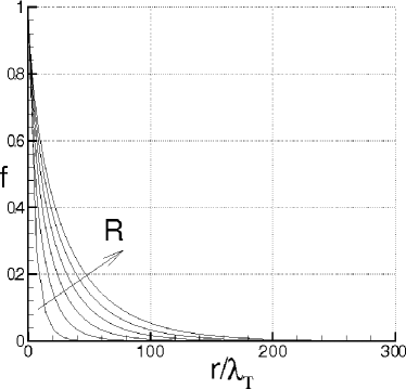
Figure 1: Longitudinal correlation function for different Taylor-Scale Reynolds numbers.

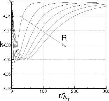
Figure 2: Longitudinal triple correlation function for different Taylor-Scale Reynolds numbers.

The cases here analyzed correspond to $R$ = $100$, $200$, $300$, $400$, $500$ and $600$. The fixed step size of the integrator scheme is selected on the basis of the asymptotic stability condition of Eq. (57). This is $\Delta\hat{r}=\sqrt{2}/R$ NAG and provides a fairly accurate description of the correlation function at small scales.

Figures 1 and 2 show the numerical solutions of Eqs. (57), where double and triple longitudinal correlation functions are both in terms of $\hat{r}$, for the different values of $R$. Due to the mechanism of energy cascade, represented by the expression of $K(r)$ (see Eq. (7)), the tail of $f$ rises with $R$ accordingly to Eq. (61) and this means that, for an assigned value of $\lambda_{T}$, all the integral scales of $f$ rise with the Reynolds number. The triple correlation function is shown in terms of $\hat{r}$ in Fig. 2. Because of energy cascade, and according to Eq. (7), $k$ decays more slowly than $f$, for $\hat{r}\rightarrow\infty$. It is apparent that assigned variations of $k$ correspond to variations of $\hat{r}$ whose size increases with $R$. The maximum of $|k|$ gives the entity of the mechanism of energy cascade. This is slightly less than 0.05 and agrees quite well with the numerous data of the literature (see Batchelor53 and Refs. therein).

Figures 3 and 4 show the plots of $E(\kappa)$ and $T(\kappa)$ calculated with Eq. (35), for the same Reynolds numbers. As the consequence of the mathematical properties of $f$, the energy spectrum behaves like $E(\kappa)=O(\kappa^{4})$ in proximity of the origin, and after a maximum is about parallel to the $-5/3$ Kolmogorov law (dashed line in Fig. 3) in a given interval of the wave-numbers. This interval defines the inertial range of Kolmogorov, and its size increases with $R$. This arises from the fact that there exists a spatial interval where $K(r)$ is about constant and, as seen, this determines that $f-1\approx r^{2/3}$. At higher wave-numbers, the energy spectrum decreases more rapidly with respect to the Kolmogorov subrange and its variations almost agree with Eq. (63). The constant $a$ of Eq. (63) varies from about 0.53 to 0.26 when $R$ assumes the values of 100 and 600, respectively. The wavenumber of separation between the two regions changes with the Reynolds number and follows the variations previously determined with Eq. (62).

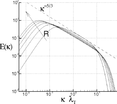
Figure 3: Turbulent Energy Spectrum for different Taylor-Scale Reynolds numbers.

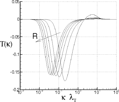
Figure 4: ”Transfer function $T(\kappa)$” for several Taylor-Scale Reynolds numbers.

Since $K$ does not modify the kinetic energy of the flow, according to Eq. (7), the integral of $T(\kappa)$ over $\kappa$ results to be identically equal to zero at all the Reynolds numbers.

In the Figs. 5 and 6, skewness and flatness of $\Delta u_{r}$ are shown in terms of $\hat{r}$ for the same values of the Reynolds numbers. The skewness $H_{3}$ is first calculated according to Eq. (8) and thereafter the flatness $H_{4}$ has been determined using Eq. (15). For a given value of $R$, $|H_{3}|$ starts from 3/7 at the origin, then decreases to small values, while $H_{4}$ starts from values quite greater than 3 at $r=0$, then reaches the value of 3. In line with Eq. (7), since $f$ decays more rapidly than $k$ as $r\rightarrow\infty$, $H_{4}$ goes to 3 more fastly than $H_{3}$ tending to zero. Although $H_{3}(0)$ does not depend upon $R$, $H_{3}(\hat{r})$ is a rising function of the Reynolds number and, in any case, the intermittency of $\Delta u_{r}$ increases with $R$ according to Eqs. (11)-(25).

Next, the Kolmogorov function $Q(r)$ and the Kolmogorov constant $C$, are determined using the previous results. According to the theory, the Kolmogorov function, defined as

$$\displaystyle Q(r)=-\frac{\langle(\Delta u_{r})^{3}\rangle}{r\varepsilon}$$ (64)

is constant with respect to $r$, and is equal to $4/5$ as long as $r/\lambda_{T}=O(1)$, where $\displaystyle\varepsilon=-3/2\ du^{2}/dt$ is the rate of the energy of dissipation. In Fig. 7, $Q(r)$ is calculated through the skewness of velocity difference and is shown in terms of $\hat{r}$. This exhibits a maximum for $\hat{r}=O(1)$ and quite small variations for higher $\hat{r}$, as the Reynolds number increases. These behavior is the consequence of the aforementioned variations of $H_{3}(r)$ with $R$ and $r$. The maximum of $Q$ rises with $R$ and seems to tend toward the limit $4/5$ prescribed by the Kolmogorov theory. In Fig. 8, the maximum of the Kolmogorov function is in term of $R$. These data (”x” symbols) are shown in comparison with those of Ref. Moisy99 (circular filled symbols and continuous line).

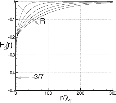
Figure 5: Skewness of $\Delta u_{r}$ at different Taylor-Scale Reynolds numbers.

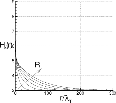
Figure 6: Flatness of $\Delta u_{r}$ at different Taylor-Scale Reynolds numbers.

There, the Kolmogorov equation with a forcing term, is compared with experimental measurements, for helium gas at low temperature. It is apparent that, for assigned $R$, the corresponding values of $Q_{max}$, calculated with Eq. (64), are less than those of Ref. Moisy99 , and such difference varies with $R$ with an average percentage value of about $12\%$. This disagreement could be due to the self-similarity here assumed or to possible differences in the estimation of the Taylor-scale. Specifically, $\lambda_{T}$ is here analytically calculated or assumed, whereas in Ref. Moisy99 , it is determined through measurement of dissipation rate. Nevertheless, the two set of data can be considered comparable, since the two variations almost exhibit the same trend.

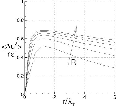
Figure 7: Kolmogorov function for several Taylor-Scale Reynolds numbers.

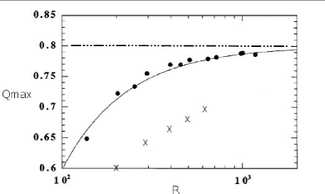
Figure 8: Maximum of the Kolmogorov Function in terms of the Taylor-Scale Reynolds number. These data are from Ref. Moisy99 . The symbols ”X” are for the present result.

Table 1: Kolmogorov constant for different Taylor-Scale Reynolds number.

$R$	$C$
100	1.8860
200	1.9451
300	1.9704
400	1.9847
500	1.9940
600	2.0005

For what concerns the Kolmogorov constant $C$, it is defined by $\displaystyle E(\kappa)\approx C{\varepsilon^{2/3}}/{\kappa^{5/3}}$, and is here calculated as

$$C=\max_{\kappa\in(0,\infty)}\frac{E(\kappa)\kappa^{5/3}}{\varepsilon^{2/3}}$$ (65)

In the table 1, the Kolmogorov constant is shown in terms of the same Reynolds numbers. The obtained values of $C$ increase with the Reynolds number and are in good agreement with the numerical and experimental values known from the various literature Kerr90 , Vincent91 , Yeung97 .

The spatial structure of $\Delta u_{r}$, expressed by Eq. (11), is also studied with the previous results. According to the various works Kolmogorov62 , Stolovitzky93 , She-Leveque94 , $\Delta u_{r}$ behaves quite similarly to a multifractal system, where $\Delta u_{r}$ obeys to a law of the kind $\Delta u_{r}(r)\approx r^{q}$ in which $q$ is a fluctuating exponent. This implies that the statistical moments of $\Delta u_{r}(r)$ are expressed through different scaling exponents $\zeta(n)$ whose values depend on the moment order $n$, i.e.

$$\left\langle(\Delta u_{r})^{n}\right\rangle=A_{n}r^{\zeta(n)}$$ (66)

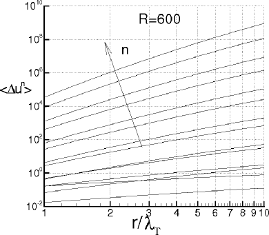
Figure 9: Statistical moments of $\Delta u_{r}$ in terms of the separation distance, for $R$=600.

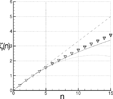
Figure 10: Scaling exponents of $\Delta u_{r}$ for several $R$. Solid symbols are for the present data. Dashed line is for Kolmogorov K41 data Kolmogorov41 . Dotted line is for Kolmogorov K62 data Kolmogorov62 . Continuous line is for She-Leveque data She-Leveque94

Table 2: Scaling exponents of the longitudinal velocity difference for several Taylor-Scale Reynolds number.

R	100	200	300	400	500	600
$\zeta(1)$	0.35	0.35	0.35	0.35	0.35	0.35
$\zeta(2)$	0.70	0.71	0.71	0.71	0.71	0.71
$\zeta(3)$	1.00	1.00	1.00	1.00	1.00	1.00
$\zeta(4)$	1.30	1.29	1.29	1.29	1.29	1.29
$\zeta(5)$	1.56	1.55	1.55	1.55	1.55	1.55
$\zeta(6)$	1.82	1.81	1.81	1.81	1.81	1.81
$\zeta(7)$	2.06	2.05	2.05	2.04	2.04	2.05
$\zeta(8)$	2.31	2.28	2.28	2.28	2.28	2.28
$\zeta(9)$	2.53	2.50	2.50	2.50	2.50	2.51
$\zeta(10)$	2.76	2.72	2.73	2.72	2.72	2.73
$\zeta(11)$	2.97	2.93	2.93	2.93	2.93	2.94
$\zeta(12)$	3.18	3.14	3.14	3.13	3.13	3.15
$\zeta(13)$	3.39	3.33	3.34	3.33	3.33	3.35
$\zeta(14)$	3.59	3.53	3.54	3.53	3.53	3.55
$\zeta(15)$	3.79	3.73	3.73	3.72	3.73	3.75

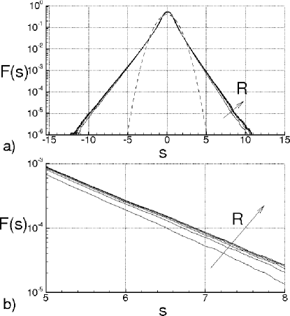
Figure 11: Probability distribution functions of the longitudinal velocity derivative for the different Taylor-Scale Reynolds numbers

In order to calculate these exponents, the statistical moments of $\Delta u_{r}$ are first calculated using Eqs. (15) for several separation distances. Figure 9 shows the evolution of the statistical moments of $\Delta u_{r}$ in terms of $\hat{r}$, in the case of $R=600$. The scaling exponents of Eq. (66) are identified through a best fitting procedure, in the intervals ($\hat{r}_{1},\hat{r}_{2}$), where the endpoints $\hat{r}_{1}$ and $\hat{r}_{2}$ have to be determined. The calculation of $\zeta(n)$ and $A_{n}$ is carried out through a minimum square method which, for each moment order, is applied to the following optimization problem

$$\displaystyle J_{n}(\zeta(n),A_{n})\equiv\int_{\hat{r}_{1}}^{\hat{r}_{2}}\displaystyle(\langle(\Delta u_{r})^{n}\rangle-A_{n}r^{\zeta(n)})^{2}dr=\mbox{min},\ n=1,2,...$$ (67)

where $(\langle(\Delta u_{r})^{n})\rangle$ are calculated with Eqs. (15), $\hat{r}_{1}$ is assumed to be equal to $0.1$, whereas $\hat{r}_{2}$ is taken in such a way that $\zeta(3)$ = 1 for all the Reynolds numbers. The so obtained scaling exponents are shown in Table (2) in terms of the Taylor scale Reynolds number, whereas in Fig. 10 (solid symbols) these exponents are compared with those of the Kolmogorov theories K41 Kolmogorov41 (dashed line) and K62 Kolmogorov62 (dotted line), and with the scaling exponents calculated by She-Leveque She-Leveque94 (continuous curve). Near the origin $\zeta(n)\simeq n/3$, and in general the values of $\zeta(n)$ are in good agreement with the She-Leveque results. In particular the scaling exponents here calculated are lightly greater than those by She-Leveque for $n>$ 8.

According to the present analysis, these peculiar laws $\zeta$ $=\zeta(n)$ which make $\Delta u_{r}$ similar to a multifractal system, are the consequence of the combined effect of the quadratic terms into Eq. (11) and of the functions $K$ and $k$ calculated through Eq. (57).

The PDFs of $\partial u_{r}/\partial{\hat{r}}$ can be formally determined with Eqs. (28) and (11). Specifically, these PDF are calculated with several direct simulations, where the sequences of the variables $\xi$, $\eta$ and $\zeta$ are first determined by a gaussian random numbers generator. The distribution function is then calculated through the statistical elaboration of the data obtained with Eq. (11). The results are shown in Fig. 11a and 11b in terms of the dimensionless abscissa

$$\displaystyle s=\frac{\partial u_{r}/\partial{\hat{r}}}{\langle\left(\partial u_{r}/\partial{\hat{r}}\right)^{2}\rangle^{1/2}}$$

These distribution functions are normalized, in order that their standard deviations are equal to the unity. The figure represents the PDF for the several $R$, and the dashed curve represents the gaussian distribution functions. In particular, Fig. 11b shows the enlarged region of Fig. 11a, where $5<s<8$. According to Eq. (11), although the skewness of $\partial u_{r}/\partial{\hat{r}}$ does not depend on $R$, the tails of PDFs change with $R$ in such a way that the intermittency of $\partial u_{r}/\partial{\hat{r}}$ rises with the Reynolds number. This increasing intermittency, caused by the quadratic terms appearing into Eq. (11), is the result of the constancy of the skewness of $\partial u_{r}/\partial{\hat{r}}$.

5 Conclusions

The obtained self–similar solutions of the von Kármán-Howarth equation with the proposed closure, and the corresponding characteristics of the fully developed turbulence are shown to be in very good agreement with the various properties of the turbulent flow from several points of view.

In particular:

• The energy spectrum follows the Kolmogorov law in a range of wave-numbers whose size increases with the Reynolds number, whereas for higher wave-numbers, it diminishes according to an exponential law.

• As the consequence of the skewness of velocity difference, the Kolmogorov function exhibits a maximum and relatively small variations in proximity of $r=O(\lambda_{T})$. This maximum value rises with the Reynolds number and seems to tend toward the limit $4/5$, prescribed by the Kolmogorov theory.

• The Kolmogorov constant moderately rises with the Reynolds number with an average value around to 1.95 when $R$ varies from 100 to 600.

• The scaling exponents of the moments of velocity difference are calculated through a best fitting procedure in an opportune range of the separation distance. The values of these exponents are in good agreement with the results known from the literature.

These results represent a further test of the analysis presented in Ref. deDivitiis2009 which adequately describes many of the properties of the isotropic turbulence.

6 Acknowledgments

This work was partially supported by the Italian Ministry for the Universities and Scientific and Technological Research (MIUR).

References

- (1) de Divitiis N., Lyapunov Analysis for Fully Developed Homogeneous Isotropic Turbulence, arXiv:0911.1463.
- (2) von Kármán, T. & Howarth, L., On the Statistical Theory of Isotropic Turbulence., Proc. Roy. Soc. A, 164, 14, 192, 1938.
- (3) Batchelor G.K., The Theory of Homogeneous Turbulence. Cambridge University Press, Cambridge, 1953.
- (4) von Kármán, T. & Lin, C. C., On the Concept of Similarity in the Theory of Isotropic Turbulence., Reviews of Modern Physics, 21, 3, 516, 1949.
- (5) Debnath L., Integral transforms and their applications, CRC Press, 1995.
- (6) Hildebrand F.B., Introduction to Numerical Analysis, Dover Publications, 1987.
- (7) Moisy F., Tabeling P., Willaime H., Kolmogorov Equation in a Fully Developed Turbulence Experiment, Phys. Rev. Lett. 82, no. 20, 3994–3997, 1999.
- (8) Kerr, R.M., Velocity, scalar and transfer spectra in numerical turbulence, J. Fluid. Mech. 211, 309 - 332, 1990.
- (9) Vincent, A. & Meneguzzi, M., The spatial structure and statistical properties of homogeneous turbulence J. Fluid. Mech. 225, 1 - 20, 1991.
- (10) Yeung P.K., Zhou Ye, Universality of the Kolmogorov constant in numerical simulation of turbulence, Phys. Rev. E 56, no. 2, 1746–1752, 1997.
- (11) Kolmogorov, A. N., Refinement of Previous Hypothesis Concerning the Local Structure of Turbulence in a Viscous Incompressible Fluid at High Reynolds Number, J. Fluid Mech. 12, 82–85, 1962.
- (12) Stolovitzky G., Sreenivasan K.R., Juneja A. , Scaling functions and scaling exponents in turbulence, Phys. Rev. E 48, no. 5, R3217-R3220, 1993.
- (13) She Z.S. and Leveque E., Universal scaling laws in fully developed turbulence, Phys. Rev. Lett. 72, 336, 1994.
- (14) Kolmogorov, A. N., Dissipation of Energy in Locally Isotropic Turbulence. Dokl. Akad. Nauk SSSR 32, 1, 19–21, 1941.