Numerical viscosity in hydrodynamics simulations in general relativity

Abstract

We present an alternative method to estimate the numerical viscosity in simulations of astrophysical objects, which is based in the damping of fluid oscillations. We apply the method to general relativistic hydrodynamic simulations using spherical coordinates. We perform 1D-spherical and 2D-axisymmetric simulations of radial oscillations in spherical systems. We calibrate first the method with simulations with physical bulk viscosity and study the differences between several numerical schemes. We apply the method to radial oscillations of neutron stars and we conclude that the main source of numerical viscosity in this case is the surface of the star. We expect that this method could be useful to compute the resolution requirements and limitations of the numerical simulations in different astrophysical scenarios in the future.

1 Introduction

There is a number of scenarios in theoretical astrophysics which need to be modelled by means of numerical simulations. The complexity found in these scenarios does not allow for a simple analytical study to explain the observations. In a subset of these scenarios the effects of general relativity are important and a Newtonian description of the system is not sufficient. Some examples of stellar size scenarios of this kind are: i) the collapse of massive stellar cores to form a neutron star, which eventually can lead to a supernova explosion, ii) for more massive stars, the collapse to a black hole and possibly an accretion disk, which can power a long-duration gamma-ray burst (GRB) according to the collapsar scenario (Woosley 1993) and could be related to the subclass of broad-lined type Ic supernovae (Modjaz et al2008), and iii) the cooling of a rapidly rotating hot proto-neutron star (PNS) to form a magnetar (Thomson & Duncan 1993). All three previous examples have in common that are quasi-spherical scenarios. Therefore it is natural to model them in numerical simulations using spherical polar coordinates.

Those scenarios have some common points. The three scenarios include multi-scale physics in which a broad range of length and time scales play an important role. In the supernova core collapse case the length scales to cover range from the size of the iron core ($\sim 1000$ km) to the size of the PNS ($\sim 10$ km). The smaller length-scale process dominating the dynamics ranges from $\sim 1$ km in the case of convectively unstable PNS formed after the collapse of the most common slow rotating progenitors (Müller & Janka 1997), to $1$ cm - $1$ m if the magneto-rotational instability develops in the collapse of fast rotating progenitors (Cerdá-Durán et al2007). Furthermore the mechanism for the explosion requires an appropriate modeling of the neutrino transport. The energy deposited by neutrinos behind the shock and the standing accretion-shock instability (SASI) probably are crucial for a successful explosion (Marek & Janka 2009). In the collapsar scenario strong rotation is necessary for the formation of a GRB. It allows the generation of an accretion disk around the formed black hole with a low-density funnel along the rotation axis. The relativistic jet which is responsible for the GRB is powered either by MHD processes or by the energy deposition of annihilating neutrinos around the axis (see e.g. MacFadyen et al2001). In the first case, magneto-rotational instabilities and dynamo processes are most probably responsible for the amplification of the magnetic field during the collapse. The case of dynamo processes in rapidly rotating PNS resembles the modeling of the sun. The cooling time-scale is of the order of seconds while the rotation period which drives the dynamo processes can be as low as $1$ ms reaching magnetic Reynolds number of $\sim 10^{17}$ (Thompson & Duncan 1993). The numerical modeling of all scenarios described above require very high resolution to resolve the MRI and the turbulence amplifying the magnetic field, full three-dimensional simulations to correctly capture the growth and saturation of the different types of instabilities (MRI, SASI, global MHD instabilities), and a time evolution much larger than the characteristic dynamical timescale of the system. Therefore the numerical methods intended to solve this problem should be as less dissipative as possible in order to guarantee that the numerical dissipation is smaller than the expected physical one or, in cases where the computational requirements do not allow this, the global properties of the system show convergence with increasing grid resolution. The numerical dissipation could be a serious limitation for the successful modeling of objects mentioned above. It is hence important to have the appropriate scaling with the resolution, which is a necessary property to have scalable numerical codes which can run efficiently in massive parallel computers.

Most of the numerical codes performing simulations of these scenarios use Eulerian grids, explicit numerical schemes, and a mesh adapted to the problem, mostly with grids in spherical polar coordinates. Eulerian grid-based codes are better suited for these scenarios than Lagrangian methods (e.g. smoothed particle hydrodynamics) because they allow to use finite-volume conservative schemes. Eulerian methods allow for the correct treatment of arbitrarily high discontinuities and shocks in general relativity (Ibañez et al2000, Dimmelmeier et al2002, Duez et al2003, Shibata 2007, Baiotti et al2007), even with magnetic fields (Gammie et al2003, Komissarov et al2005, Anninos et al2005, Antón et al2006). Explicit methods are better suited for multidimensional simulations since they are computationally less expensive and easier to parallelize, although they have time-step limitations given by the CFL condition (Courant et al1928, 1967). Spherical polar coordinates have several properties which make them appropriate to model the objects described above: i) are well adapted for quasi-spherical objects, ii) allow for accurate conservation of angular momentum, which is not true, in general, for Eulerian grids (see e.g. Zink et al2008 and Fragile et al2009), iii) axisymmetry and spherical symmetry can be easily enforced, and iv) large radial domains can be covered using non equally spaced radial grids. These numerical methods have been successfully applied in 1D (spherical symmetry) and 2D (axisymmetry) simulations. However the extension to 3D in spherical coordinates suffers from severe time-step restrictions which render simulations unaffordable unless a special treatment of the central and polar regions is used (see. e.g Müller & Janka 1997)

Numerical dissipation effects are present in simulations using Eulerian grids due to the discretization of the equations that are solved. There are several methods to quantify the amount of numerical dissipation of a code based on the measure of the energy losses of the system. This has been standard practice since the first studies of hydrodynamic turbulence (e.g. Herring et al1974) due to the necessity of resolving the physical dissipation scales. There are also studies of the decay of waves in hydrodynamics (Porter et al1994) and MHD simulations (e.g. Simon & Hawley 2009). More recently the numerical dissipation has been estimated measuring the angular momentum transport by MHD turbulence (Fromang & Papaloizou 2007, Simon et al2009). All these methods allow for a simplified numerical setup in where the local dissipation properties of the numerical algorithms can accurately be estimated. We propose an alternative approach to measure the numerical dissipation that is suitable for global simulations of relativistic stars close to the equilibrium.

The aim of this paper is to study the effects of numerical viscosity in simulations with spherical coordinates and study the influence of the grid resolution and the numerical scheme. In section 2 we describe the hydrodynamics equations including physical bulk viscosity in general relativity (GR), in section 3 we present a method to estimate numerical dissipation effects in a simplified test case. We apply this method in section 4 to estimate the numerical viscosity of oscillating neutron stars. We finish the paper in section 5 discussing the implications of our numerical results. If is not explicitly mentioned, we use units in which $c=G=1$. Greek indices run from $0$ to $3$ and Latin indices from $1$ to $3$.

2 GR hydrodynamics with bulk viscosity

We use the 3+1 decomposition of the spacetime in which the metric reads

$$ds^{2}=g_{\mu\nu}\rmd x^{\mu}\rmd x^{\nu}=-\alpha^{2}\,dt^{2}+\gamma_{ij}(dx^{i}+\beta^{i}\,dt)(dx^{j}+\beta^{j}\,dt),$$ (1)

where $\alpha$, $\beta^{i}$ and $\gamma^{ij}$ are the lapse function, the shift vector and the spatial 3-metric respectively. In addition we consider the conformally flat condition (CFC) approximation (Isenberg 2008, Wilson et al1996) for the 3-metric $\gamma_{ij}=\phi^{4}f_{ij}$, where $\phi$ is the conformal factor and $f_{ij}$ the flat 3-metric in spherical coordinates. This approximation uses the maximal slicing condition and quasi-isotropic coordinates as gauge conditions. Under this approximation the resulting system consist in a hierarchy of elliptic equations (Cordero-Carrión et al2009).

To be able to study numerical dissipation effects we need a physical counterpart to calibrate our results. We use for this purpose the bulk viscosity of the fluid. The energy momentum tensor of a fluid with bulk viscosity (Ehlers 1961) is

$$T^{\mu\nu}=\rho(1+\epsilon)u^{\mu}u^{\nu}+(P-\zeta\Theta)h^{\mu\nu},$$ (2)

where $\rho$ is the rest-mass density, $\epsilon$ is the specific internal energy, $u^{\mu}$ is the 4-velocity of the fluid, $P$ is the pressure, $\zeta$ is the bulk viscosity, $\Theta\equiv u^{\mu}_{;\mu}$ is the expansion of the fluid and $h^{\mu\nu}\equiv g^{\mu\nu}+u^{\mu}u^{\nu}$. The bulk viscosity appears as an isotropic term in the energy-momentum tensor in a very similar way to the pressure. Therefore we can define a modified pressure $\hat{P}\equiv P-\zeta\Theta$ such that the energy-momentum tensor has the same form as a perfect fluid

$$T^{\mu\nu}=\rho\hat{h}u^{\mu}u^{\nu}+\hat{P}g^{\mu\nu},$$ (3)

where $\hat{h}\equiv h-\zeta\Theta/\rho$, being $h\equiv 1+\epsilon+P/\rho$ the relativistic specific enthalpy. Using this form of the energy-momentum tensor is easy to modify an existing hydrodynamics code to include bulk viscosity, specially if the next assumptions are taken into account: i) we approximate the expansion assuming a post-Newtonian expansion and small perturbations,

$$\Theta=\bi{\nabla}\cdot\bi{u}+\mathcal{O}(c^{-2})+\mathcal{O}(v^{2}),$$ (4)

where $\mathcal{O}(c^{-2})$ corresponds to first post-Newtonian corrections. All the simulations that we run with physical bulk viscosity in this work belong to this regimen. ii) The bulk viscosity coefficient $\zeta$ is sufficiently small, such that $\hat{P}>0$. And iii) we neglect the contribution of the bulk viscosity in the computation of the sound speed needed for our numerical scheme.

The hydrodynamics equations with bulk viscosity can be cast as a system of conservation laws (cf. Ibañez et al2000)

$$\partial_{t}\left(\sqrt{\gamma}D\right)+\partial_{i}\left[\sqrt{\gamma}Dv^{*i}\right] = 0,$$ (5)

$$\partial_{t}\left(\sqrt{\gamma}S_{j}\right)+\partial_{i}\left[\sqrt{\gamma}\left(S_{j}v^{*i}+\delta^{i}_{j}\alpha\hat{P}\right)\right] = \frac{1}{2}\alpha\sqrt{\gamma}T^{\mu\nu}\,\partial_{j}g_{\mu\nu},$$ (6)

$$\partial_{t}\left(\sqrt{\gamma}\tau\right)+\partial_{i}\left[\sqrt{\gamma}\left[\tau v^{*i}+\alpha\hat{P}v^{i}\right)\right] = \alpha^{2}\sqrt{\gamma}\left(T^{\mu 0}\partial_{\mu}(\ln{\alpha})-T^{\mu\nu}\Gamma^{0}_{\mu\nu}\right)$$ (7)

where $D\equiv\rho W$, $S_{j}\equiv\rho\hat{h}W^{2}v_{j}$, $\tau\equiv\rho\hat{h}W^{2}-\hat{P}-D$ are the conserved variables, $v^{*i}\equiv\rmd x^{i}/\rmd t$ is the coordinate 3-velocity, $v^{i}=(v^{*i}-\beta^{i})/\alpha$ is the 3-velocity as measured by an Eulerian observer, and $W=1/\sqrt{1-\gamma_{ij}v^{i}v^{j}}$ the Lorentz factor. In the non-relativistic limit the equations for a classical viscous fluid can be recovered (Landau & Lifschitz 1987) which for constant $\zeta$ result in the Navier-Stokes equations.

We solve the coupled system of CFC spacetime evolution and GR hydrodynamics equations using the numerical code COCONUT (Dimmelmeier et al2002, 2005). The numerical code uses standard high-resolution shock-capturing schemes for the hydrodynamics evolution in spherical polar coordinates, and spectral methods for the spacetime evolution.

3 Estimating numerical viscosity

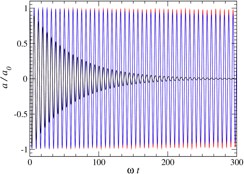
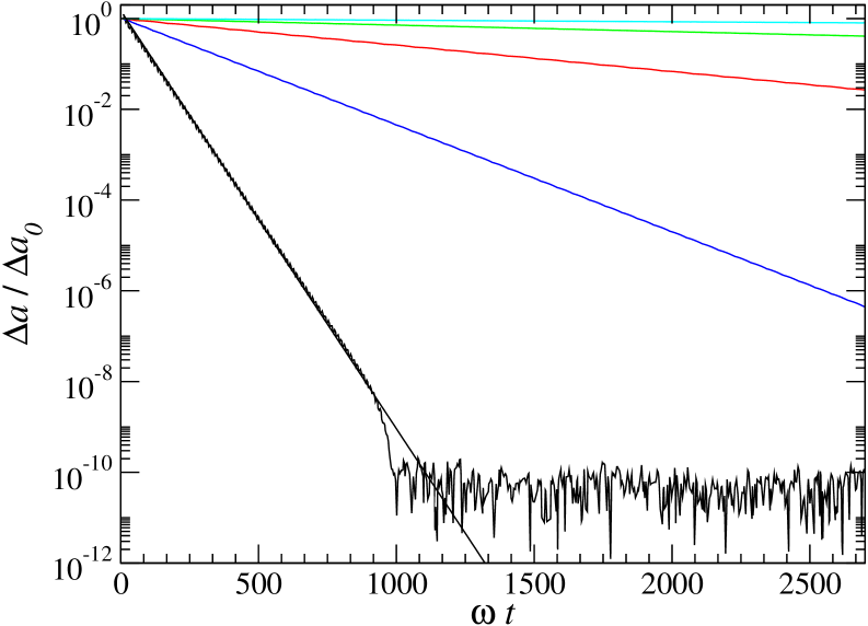
Figure 1: Time evolution of the first oscillation mode in the spherical test system. All evolutions shown are computed using the Marquina flux formula. Left panel shows the evolution of the perturbation $a$ normalized to its initial value $a_{0}$ for a radial resolution $n_{r}=80$ and different reconstruction procedures: constant (black line), minmod (blue line) and MC (red line). The right panel shows the evolution of the amplitude of the perturbation $\Delta a$ normalized to its initial value $\Delta a_{0}$ using minmod reconstruction and different resolutions: $10$ (black), $20$ (blue), $40$ (red), $80$ (green) and $160$ (cyan). We also plot the fit of the lowest resolution simulation to an exponential decay (black line).

To estimate the numerical viscosity of our code we have designed a simple spherical test. We consider a spherical fluid system of radius $R$ and constant density in a static Minkowski spacetime. This system allow for discrete modes of radial oscillations (see appendix A). Since the eigenfunctions of the modes are known it is possible to excite very accurately single modes of the system and follow their evolution. We evolve the system using a polytropic equation of state, therefore, since the system is adiabatic, there are no possible energy losses and the oscillations should keep constant amplitude as long as non-linear effects does not appear. Hence, any damping observed in the numerical simulation has to be caused by numerical dissipation effects.

We have chosen a system with $R=1$ and initial density $\rho_{0}=1$. The equation of state is a polytrope of the form $P=K\rho^{\Gamma}$ with $\Gamma=4/3$ and $K=1/3\times 10^{-3}$. We use a perturbation $A(r)$ (see appendix A) of the velocity with an amplitude of $v^{\prime}_{0}=10^{-5}$ corresponding to the lowest frequency mode, $\omega=0.094$. This amplitude is sufficiently small for the oscillations to be considered linear. We have used second order Runge-Kutta method for the time evolution in all cases and two different flux formulae, Marquina (Donat el al 1998) and HLL (Harten & van Leer 1983). We have computed all models using different reconstruction techniques (constant and linear with minmod or MC slope limiters) and different resolutions ($n_{r}=10$, $20$, $40$, $80$ and $160$). We have also computed the models without physical bulk viscosity ($\zeta=0$) and with non-zero values ($\zeta=10^{-4}$, $10^{-5}$ and $10^{-6}$). We have evolved the system for $2700\,\omega^{-1}$. To follow the evolution of the oscillations we computed the quantity

$$a(t)=\int\rmd x^{3}A(r)v^{r}(r,t).$$ (8)

Left panel of figure 1 shows the time evolution of $a/a_{0}$ for different reconstruction procedures, $a_{0}$ being the initial value of $a$. The oscillation frequency coincides with the predicted by the linear analysis within $0.1\%$ for $n_{r}=80$ . It can be seen that the order of the reconstruction has a strong influence in the numerical damping of the system, being much stronger for first order reconstruction (constant) than for second order (minmod or MC). In order to quantify this effect we estimate the damping time for each simulation as it is described next. In every case, we first compute the amplitude of $a$ as the difference between two consecutive oscillations, $\Delta a$. In the right panel of figure 1 we plot the evolution of the amplitude for the minmod reconstruction case for five different resolutions. For very low resolution, the amplitude of the perturbation falls bellow the round-off error of the code within the duration of the simulation and it saturates. We fit next the the amplitude of the oscillations to an exponential decay $\Delta a(t)=\Delta a(0)\,\rme^{-2t/\tau}$ for each model. This procedure allow us to compute the value of the damping time of the amplitude, $\tau/2$. Since the energy of the perturbations scales quadratically with the velocity, the damping time of the energy is $\tau$. Finally, using (33) it is possible to compute the physical bulk viscosity from the value of $\tau$ as

$$\zeta=\frac{\zeta_{\rm dyn}}{\omega\,\tau},$$ (9)

where $\zeta_{\rm dyn}\equiv 2\rho_{0}c_{s}^{2}/\omega$ and $c_{s}$ is the sound speed. The left panel of figure 2 shows the behavior of the numerical viscosity with the radial resolution for the different numerical schemes tested in simulations without physical bulk viscosity ($\zeta=0$). To check the scaling with resolution we fit the viscosity values to a power law

$$\frac{\zeta}{\zeta_{\rm dyn}}=S\left(\frac{\Delta x}{\lambda}\right)^{p},$$ (10)

where $\lambda=2\pi c_{\rm s}\omega^{-1}$ is the wavelength of the oscillation mode, being $c_{\rm s}$ the speed of sound. The results of the fitted parameters $S$ and $p$ for the different numerical methods are shown in table 1. In all cases $S$ is of order one, although in general the Marquina flux formula provides about $30\%$ less bulk viscosity than the same simulation with HLL. The scaling does not change substantially with the flux formula but only with the reconstruction scheme: for constant reconstruction we recover first order convergence and for linear reconstruction (minmod and MC) second order. These fits allow us to compute the numerical bulk viscosity of different numerical schemes.

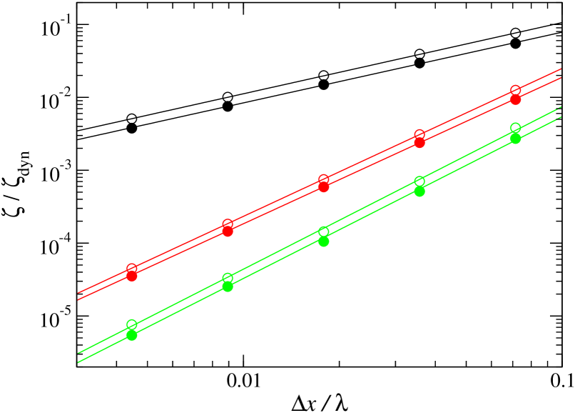
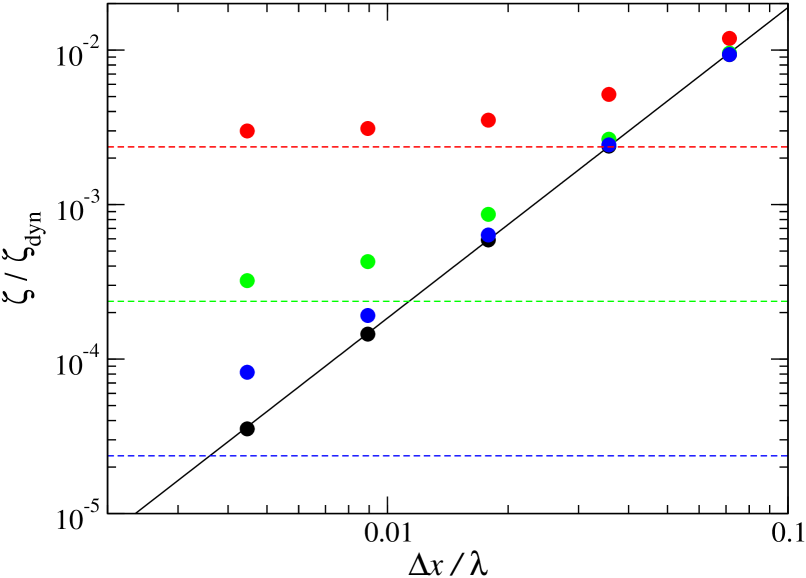
Figure 2: Dependence of the numerical viscosity $\zeta$ with the resolution in the case of the test sphere. The left panel shows the case without physical bulk viscosity for different flux formulae, Marquina (filled circles) and HLL (open circles), and different reconstruction schemes, constant (back), minmod (red) and MC (green). The right panel shows the case with Marquina flux formula and MC reconstruction for different values of the physical viscosity $\zeta=10^{-4}$ (red) $10^{-5}$ (green), $10^{-6}$ (blue) and $0$ (black). Dashed lines of the same color correspond to the value of the physical viscosity in each case.

In the right panel of figure 2 we consider the simulations with physical bulk viscosity ($\zeta\neq 0$). In this case the viscosity of the code decreases with resolution with a similar scaling as in the case without physical viscosity. For sufficiently high resolution, the viscosity converges to the value of the added physical viscosity. Our method to estimate the bulk viscosity overestimates, in the convergent regime, the real physical viscosity by $\sim 25\%$. We have checked that the damping time and therefore the viscosity is not affected for a wide range of amplitudes of the perturbation ($0.1$-$10^{-7}$) and hence we can conclude that non-linear effects does not play any role in the damping observed during this test. We have also checked that the results are independent of the CFL factor used for the time-step, by changing its value between $0.8$ and $10^{-3}$. Since our final aim is to perform multidimensional simulations we have also performed some axisymmetric 2D models of this spherical system. We have chosen two representative radial resolutions $n_{r}=20$ and $80$ and varied the angular resolution $n_{\theta}=8$, $16$ and $32$. In all cases the results are indistinguishable from the 1D spherical simulations with the same number of radial points.

Table 1: Coefficients $S$ and $p$ of the fitted numerical viscosity in radial oscillations of a test fluid sphere, for different flux formulae and reconstruction schemes.

• Flux formula	reconstruc.	$p$	$S$
  Marq.	constant	0.97	0.74
  HLL	constant	0.98	1.06
  Marq.	minmod	2.01	1.91
  HLL	minmod	2.03	2.66
  Marq.	MC	2.23	0.96
  HLL	MC	2.23	1.28

4 Numerical damping of neutron stars

We apply our method to estimate viscosity in the case of radial oscillations of non-rotating neutron stars. Our initial model is a non-rotating relativistic equilibrium configuration (Tolman 1939, Oppenheimer & Volkoff 1939). We use a polytropic equation of state $P=K\rho^{\Gamma}$ with adiabatic index $\Gamma=2$ and polytropic constant $K=100$ (units of $G=c=M_{\odot}=1$). We choose central rest mass density to be $\rho_{\rm c}=7.9\times 10^{14}$ g cm^-3 and gravitational mass $M_{\rm g}=1.4M_{\odot}$. The resulting circumferential radius is $R_{\rm C}=14.16$ km, and the isotropic radial coordinate at the surface of the star is $R=12.0$ km. We evolve the system in dynamic spacetime adding an initial perturbation of the radial velocity corresponding to the fundamental radial oscillation mode with an amplitude of $10^{-3}$. To compute the eigenfunction of the fundamental mode necessary for the perturbation, we use the eigenfunction recycling technique described in Dimmelmeier et al2006. We perform 1D spherical simulations with different radial resolutions of the fluid grid, $n_{r}=80$, $160$, $320$ and $640$, which is equally spaced from the center to 14.4 km. The time-step is computed using the CFL condition for the eigenvalues of the hydrodynamics system, resulting in $\Delta t=1.13\times 10^{-3}$ ms for a grid with $n_{r}=80$ and a CFL factor 0.8. We use an artificial atmosphere to treat the vacuum surrounding the star as described in Dimmelmeier et al2002. The treatment consists of resetting all numerical cells with $\rho$ bellow a certain threshold to the value $\rho_{\rm atm}$ and setting the velocity to zero. The values for the threshold and the atmosphere are $10^{-6}$ and $10^{-10}$ times the initial central density respectively. We have checked that the results presented here do not change if we decrease the values of these two quantities. We use three radial domains for the spectral metric solver: two including the star and one compactified domain in the exterior. Each of the domains has either $17$ or $33$ collocation points for our low and high metric resolution simulations. Since the CFC approximation only contains elliptic equations, which are not restricted by the CFL condition, it is not necessary to solve the metric as frequently as the hydrodynamics equations. We use a metric computation rate of $n_{r}/8$, i.e. we compute the metric once every $n_{r}/8$ time step of the hydrodynamics. We use a parabolic extrapolation of all the metric quantities between consecutive metric computations, which has been shown to provide sufficient accuracy during the evolution (Dimmelmeier et al2002). We do not add physical bulk viscosity in any of the simulations ($\zeta=0$), therefore the only dissipative processes in the evolution are of numerical nature. To compute the numerical bulk viscosity we use (9) as in the previous section but with $\zeta_{\rm dyn}\equiv 2{\bar{\rho}}_{0}c_{s}^{2}/\omega$ according to (38), where $\bar{\rho}$ is estimated as the central density. Since the numerical viscosity can depend on the location in the star the resulting value represents an average numerical viscosity. For our particular case and the fundamental radial mode ($\omega=9.11\times 10^{3}$ Hz) the resulting value is $\zeta_{\rm dyn}=3.99\times 10^{31}$ g cm^-1 s^-1. This procedure gives us an idea of the order of magnitude of the averaged numerical viscosity on the star. More accurate computations of the damping-time could be done using the expressions of the appendix B or the procedure described in Cutler et al1990.

Figure 3 shows the variation of the viscosity with the radial resolution normalized to the wavelength of the perturbation computed at the center of the star. In general the viscosity decreases with increasing resolution. However the lowest resolution case with the minmod reconstruction shows an anomalously low numerical viscosity, which we think is an artifact of the low resolution. We plot the function $\zeta/\zeta_{\rm dyn}=\Delta r/\lambda$ for comparison. The general trend is roughly first order decreasing the order for the highest resolution models, although we are using both first and second reconstruction schemes. The reason for the lower order of convergence is that all reconstruction schemes reduce to first order at discontinuities. Since we encounter a discontinuity at the surface any evolution will inevitably lead to first order convergent results. This is also a strong indication that the main numerical dissipation process in the neutron star evolution is probably due to the surface of the star, and therefore increasing the reconstruction order does not decreases the mean numerical viscosity responsible for the damping of global oscillations.

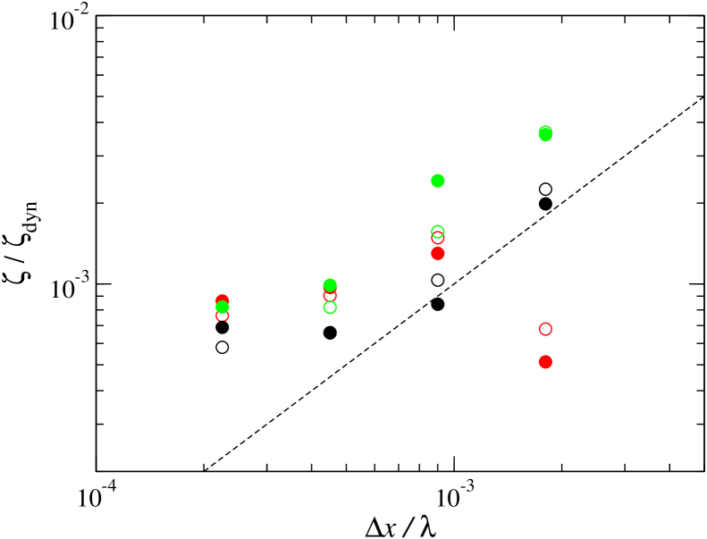
Figure 3: Dependence of the numerical viscosity $\zeta$ on the resolution in neutron star evolution. We show values for different flux formulae, Marquina (filled circles) and HLL (open circles), and different reconstruction schemes, constant (back), minmod (red) and MC (green). In all cases the highest metric resolution case is plotted. The dashed line represents the function $\zeta/\zeta_{\rm dyn}=\Delta r/\lambda$.

We have checked the influence of the CFL factor, the metric calculation rate and the 2D effects for simulations with $n_{r}=80$ radial points, Marquina flux formula and MC reconstruction. One of the main differences with respect to the spherical test case of the previous section is that the equations that we are solving have sources due to the gravity terms. In general the presence of non-zero sources can increase the stiffness of the problem leading to inaccurate solutions, even unstable for extremely stiff sources. We expect some influence of the CFL factor in our simulations since the reduction of the time step tends to cure the stiffness problems. We have performed simulations with CFL factor $0.8$ (standard for all previous simulations), $0.1$, $0.01$ and $0.001$, with a metric computation rate of $10\times 0.8/{\rm(CFL\,factor)}$, which maintain constant the metric computation rate per unit evolution time. The amplitude of the oscillation at the end of the simulation varies about $0.5\%$ at most. However most of the variation is observed between CFL factor $0.8$ and $0.1$, and decreasing the CFL factor further does not significantly changes the solution. Therefore the effect on the computed damping rate can be neglected. We find that the stiffness of the sources depends on how often the metric is computed. We also perform the same simulations with a metric computation rate $10$. In this case the metric is computed more often per time unit than the previous one, as the CFL factor decreases. We find variations of about $25\%$ in the final amplitude depending on the CFL factor used, although these variations depend strongly on the radial resolution. For $n_{r}=160$ the maximum variation due to CFL factor changes is smaller than $10\%$. Since the effect of the CFL factor becomes larger lowering the metric computation rate, we can conclude that the sources become more stiff if the metric is computed more often. An explanation for this effect is that if the metric is computed less often, the sources vary due to the space-time evolution on time-scales longer, than the hydrodynamic variables, which reduces the stiffness. We conclude that the stiffness of the sources is not significantly affecting the computation of the damping rates for the metric computation rate that we use in our regular simulations. However special care should be taken in simulations in which the metric computation rate is high (close to one), e.g. in black hole formation simulations, since the stiffness of the sources could lead to an increasing of the numerical viscosity of the code if the CFL factor is not appropriately lowered. We also perform 2D-axisymmetric simulations with $4$, $8$ $16$ and $32$ angular grid points. Since the initial perturbation is radial, non-radial modes are not excited. We find an error in the angular velocity which is of order $v^{\theta}/v^{r}\approx 10^{-9}$, and which is closely related to the accuracy of numerical recovery of the primitive variables. Since the angular extension of the grid restricts the time step of the simulation in a factor proportional to $1/n_{\theta}$, we find a similar behaviour increasing $n_{\theta}$ as it is found decreasing the CFL factor.

5 Discussion

We conclude that it is possible to estimate dissipation effects in numerical simulations which produce an effect similar to physical bulk viscosity. In a very simplified case, as the test fluid sphere of constant density, the numerical viscosity scales with the order of the reconstruction. In the application of our method to neutron stars simulations we find that the behaviour of the numerical viscosity is more complicated since the gravity sources also contribute to the numerical dissipation processes, and the presence of the surface lowers the scaling of the viscosity to first order.

To understand why the numerical inaccuracies can be modelled as a bulk viscosity term we consider the generic form of the flux formula in a Riemann solver

$$F^{i}_{\rm num}=\bar{F}^{i}+\Lambda\Delta U,$$ (11)

where $F^{i}_{\rm num}$ is the numerical flux that is used in the time update, $\bar{F}^{i}$ is an averaged value of the flux, $\Delta U$ represents the discontinuity at each cell interface and $\Lambda$ the eigenvalue matrix. The particular form of the average and the matrix $U$ depends on the particular Riemann solver. If a reconstruction scheme of order $p$ is used, the value of $U$ at both sides of the interface in smooth regions of the flow agrees up to the $p-1$-th derivative, therefore for any function $f(U)$

$$\Delta f(U)\propto\left(\Delta r\right)^{p}{\mathcal{D}}^{p}U$$ (12)

where ${\mathcal{D}}^{p}$ represents $p$-th spatial derivatives. If one applies this expression to the momentum equation

$$\partial_{t}\left(\sqrt{\gamma}S_{j}\right)+\partial_{i}\bar{F}^{i}+\mu\,(\Delta r)^{p}\,{\mathcal{D}}^{(p+1)}S_{j}=Q,$$ (13)

where $\mu$ depends on the specific Riemann solver used and $Q$ represent the sources (r.h.s of (15)). The new term appearing in the numerical version of the equations is a dissipative term since in includes a $p+1$ derivative, while $\mu\,(\Delta r)^{p}$ is the corresponding dissipative coefficient. For first order reconstruction, the dissipation term includes second derivatives that resemble to a viscosity term with viscosity proportional to $\Delta r$. For higher order reconstruction the new term resembles hyperviscosity coefficients. Note that with this interpretation we can identify the computed value of $\zeta$ in our simulations with a viscosity or hyperviscosity term, which scales with resolution with the order of the reconstruction scheme. Furthermore, we can argue that, since the new terms in (13) are responsible for both the bulk viscosity and shear viscosity terms, the value of the numerical shear viscosity of the code has to be of the same order of magnitude as the numerical bulk viscosity estimated in this work. If this case were true, the method described in this paper could be a powerful tool to estimate numerical dissipative effects in multidimensional simulations . However the method has some limitations due to the approximations that we considered. The integral expressions (36) and (37) as well as the approximate expression for the expansion (4) rely on the facts that a post-Newtonian expansion is possible and that velocity perturbations are small. This provides an order-of-magnitude estimate in the case of systems involving neutron stars or proto-neutron stars since $\mathcal{O}(c^{-2})\sim 0.15$. In this scenarios the velocity involved in oscillations is typically smaller than $0.1$. In the vicinity of black holes, the post-Newtonian expansion is not convergent anymore, and the method can lead to large inaccuracies. Similar thing happens in the case of flows with a high Lorentz factor as those observed in jets.

From our simulations we also conclude that the gravity can be an important source of numerical viscosity which has to be estimated in an appropriate way. The stiffening of the sources in the presence of rapidly changing spacetime, can lead to a strong increasing in the numerical viscosity if the CFL condition is not adapted accordingly. Although this effect is not a problem in the simulations presented in this work, it could be in case in which the spacetime evolves in similar time-scales as the fluid, e.g. in the formation of a black hole. It is therefore important to test in the future which are the real effects of numerical viscosity in such simulations.

Finally, we note that all the viscosity results given in this paper are normalized to $\zeta_{\rm dyn}$, which depends on the frequency of the oscillation $\omega$. For a given astrophysical scenario, and the same numerical resolution, different modes will be affected in a different way depending on the frequency of the mode. Therefore, in order to estimate the resolution needed to evolve a system for a given amount of time with reasonably small damping one has to use the mode with higher frequency, of those who may be important in the dynamics of the system. Deciding which is this mode may be non trivial in non-linear simulations, since a strong numerical damping in high frequency modes, which are coupled to the lower frequency modes, can modify the damping times for the low frequency modes too.

Appendix A Radial oscillations of an homogeneus sphere.

We consider a spherically symmetric barotropic fluid in Minkowski spacetime, with equation of state $P=P(\rho)$. The hydrodynamics equations (14) and (15) in this case read:

$$\partial_{t}\left(\rho W\right)+\frac{1}{r^{2}}\partial_{r}\left[r^{2}\rho Wv\right] = 0,$$ (14)

$$\partial_{t}\left(\rho\hat{h}W^{2}v\right)+\frac{1}{r^{2}}\partial_{r}\left[r^{2}\rho\hat{h}W^{2}v^{2}\right] = -\partial_{r}\hat{P},$$ (15)

where $v\equiv v^{r}$. The equilibrium solution of this system is trivially zero velocity, $v_{0}=0$, and constant pressure, $P=P_{0}$, and hence constant rest mass density, $\rho=\rho_{0}$. We consider perturbations of the rest mass density and velocity, $\rho=\rho_{0}+\rho^{\prime}$ and $v=v^{\prime}$, and hence

$$P = P_{0}+\,\frac{\partial P_{0}}{\partial\rho_{0}}\,\rho^{\prime}=P_{0}+h_{0}\,c_{s}^{2}\,\rho^{\prime}.$$ (16)

where $c_{s}^{2}$ is the speed of sound of the equilibrium model. The linearized hydrodynamics equations read

$$\partial_{t}v^{\prime}+\frac{c_{s}^{2}}{\rho_{0}}\partial_{r}\rho^{\prime}-\frac{\zeta}{\rho_{0}h_{0}}\partial_{r}\Theta = 0,$$ (17)

$$\partial_{t}\rho^{\prime}+\rho_{0}\partial_{r}v^{\prime}+\frac{2}{r}\rho_{0}v^{\prime} = 0,$$ (18)

If $\zeta$ is sufficiently small, i.e. $\zeta<<h_{0}\rho_{0}$, the viscosity terms can be neglected in the computation of the perturbations spectrum. In this case equations (17) and (18) can be combined in a wave equation for $\rho^{\prime}$

$$\partial_{tt}\rho^{\prime}-c_{s}^{2}\partial_{rr}\rho^{\prime}-\frac{2c_{s}^{2}}{r}\partial_{r}\rho^{\prime}=0.$$ (19)

The system of equations (17) and (18) admits oscillatory solutions of the form $v^{\prime}=A(r)\,\sin{\omega t}$ and $\rho^{\prime}=B(r)\,\cos{\omega t}$ and hence (19) results in

$$\partial_{rr}B+\frac{2}{r}\partial_{r}B+\frac{\omega^{2}}{c_{s}^{2}}B=0.$$ (20)

This equation has the form of the Lane-Emden equation of index 1, which have solutions regular at $r=0$ (Chandrasekhar 1967) of the form

$$B(r)=\rho^{\prime}_{0}\frac{\sin{(k\,r)}}{k\,r},$$ (21)

where $k=\omega/c_{s}$ and $\rho^{\prime}_{0}$ is a parameter which controls the amplitude of the density perturbation. From (17) the solution for the velocity perturbation is

$$A(r)=v^{\prime}_{0}\,\frac{k\,r\cos{(k\,r)-\sin{(k\,r)}}}{(k\,r)^{2}},$$ (22)

where $v^{\prime}_{0}$ controls the amplitude of the velocity perturbation and is related to $\rho^{\prime}_{0}$ by

$$\frac{\rho^{\prime}_{0}}{\rho_{0}}=-\frac{v^{\prime}_{0}}{c_{s}}.$$ (23)

If we impose boundary conditions at the surface $v^{\prime}(R)=0$, i.e., $A(R)=0$ we find a discrete spectrum of modes given by the solutions of

$$\tan{(k\,R)}=k\,R.$$ (24)

We have computed the roots of this equations by means of a bisection algorithm. The first five numerical solutions correspond to $k\,R=4.49$, $7.73$, $10.90$, $14.07$ and $17.11$.

Appendix B Damping time of an oscillating spherical star

The rate of change of the energy due to bulk viscosity of a pulsating star is (cf. Cutler et al1990)

$$\frac{\rmd E}{\rmd t}=-4\pi\int_{0}^{R}\rmd r\,r^{2}\phi^{6}\,\zeta|\Theta|^{2},$$ (25)

and, provided that the energy of the pulsations $E$ is known, the damping time is

$$\tau=-2E\left<\frac{\rmd E}{\rmd t}\right>^{-1}.$$ (26)

where $<>$ denotes the time average over a cycle.

The energy stored in the radial oscillations of a spherical star can be computed as the energy difference between the star in equilibrium and the perturbed system. Previous computations (Meltzer & Thorne 1966, Glass & Lindblom 1983) used Schwarzschild coordinates in their computations. Instead of performing the coordinate transformation to the choice of the present work we find it easier and more instructive to compute the energy of the oscillations directly in our coordinates, although the result should be identical.

The ADM energy is a conserved quantity which in spherical symmetry and under our gauge choice is

$$E_{\rm ADM}=-2\int_{0}^{R}\rmd r\,r^{2}\Delta\phi=4\pi\int_{0}^{R}\rmd r\,r^{2}\phi^{5}\left(\rho hW^{2}-P+\frac{K_{ij}K^{ij}}{16\pi}\right),$$ (27)

being $\Delta$ the Laplacian with respect to the flat 3-metric and $K_{ij}$ the extrinsic curvature of the induced 3-metric $\gamma_{ij}$. Since the extrinsic curvature vanishes for the equilibrium system in our gauge choice the equilibrium ADM energy is

$$E_{\rm ADM\,0}=4\pi\int_{0}^{R}\rmd r\,r^{2}\phi_{0}^{5}(\rho_{0}h_{0}-P_{0}).$$ (28)

The ADM energy does not change with time and hence we can compute its value by evaluating the integral at the oscillation phase with maximum velocity. In this phase, due to the continuity equation (14), the variation of $\phi^{6}\rho W$ with respect to the equilibrium is zero. The leading term in the perturbation corresponds to quadratic terms in the velocity. The energy of the oscillations is thus $E=E_{\rm ADM}-E_{\rm ADM\,0}$ which results in

$$E= 4\pi\int_{0}^{R}\rmd r\,r^{2}\phi_{0}^{5}\left[\rho_{0}h_{0}\frac{1}{2}{v^{\prime}}^{2}-(\rho_{0}h_{0}-5P_{0})\frac{\phi^{\prime}}{\phi}+\frac{{K^{\prime}}_{ij}{K^{\prime}}^{ij}}{16\pi}\right]$$ (29)

for adiabatic perturbations. Note that here $\phi^{\prime}=\phi-\phi_{0}$ corresponds to the variation of $\phi$ with respect to the equilibrium for the phase in which $v^{\prime}$ is maximum and hence is a term quadratic in $v^{\prime}$.

If we apply this expressions to the case of the spherical fluid in Minkowski spacetime of the appendix A the resulting expressions are

$$E=4\pi\int_{0}^{R}\rmd r\,r^{2}\frac{1}{2}\rho_{0}A(r)^{2}=\rho_{0}{v^{\prime}}^{2}_{0}\pi\frac{R}{k^{2}}\sin^{2}{(k\,R)},$$ (30)

$$\left<\frac{\rmd E}{\rmd t}\right>=-\zeta{v^{\prime}}^{2}_{0}\pi R\sin^{2}{(k\,R)},$$ (31)

where we have explicitly used that (24) is fulfilled to perform the integration and that $<|\Theta|^{2}>=(\nabla A)^{2}/2=\omega^{2}B^{2}/(2\rho_{0}^{2})$. The damping time is therefore

$$\tau=\frac{2\rho_{0}c_{s}^{2}}{\zeta\omega^{2}},$$ (32)

It is convenient to express it as

$$\omega\tau=\frac{\zeta_{\rm dyn}}{\zeta}$$ (33)

where $\zeta_{\rm dyn}\equiv 2\rho_{0}c_{s}^{2}/\omega$. For $\zeta\sim\zeta_{\rm dyn}$ the damping of the mode occurs in dynamical time-scales, while if $\zeta<<\zeta_{\rm dyn}$ the damping occurs in secular timescales.

In the case of a perturbed relativistic star the computation of the damping rate can not be computed analytically. However we can still make an order of magnitude estimation. For this purpose it is useful to truncate the equations (25) and (29) to the leading order in the post-Newtonian expansion

$$E = 4\pi\int_{0}^{R}\rmd r\,r^{2}\frac{1}{2}\rho_{0}{v^{\prime}}^{2}(1+\mathcal{O}(c^{-2})),$$ (34)

$$\frac{\rmd E}{\rmd t} = -4\pi\int_{0}^{R}\rmd r\,r^{2}\,\zeta|\Theta|^{2}\left(1+\mathcal{O}(c^{-2})\right).$$ (35)

which corresponds to the Newtonian expression for the kinetic energy, beging $\mathcal{O}(c^{-2})\sim\mathcal{O}(v^{2})\sim\mathcal{O}(GM/R)$ the first post-Newtonian corrections (see e.g. Blanchet et al1980). If we assume $e^{i(\omega t+kr)}$ dependence of the perturbations, where $k$ is the wavenumber, then $<|\Theta|^{2}>\sim k^{2}<v^{2}>=k^{2}v_{\rm max}^{2}/2$. The energy and energy losses result in this case

$$E=2\pi\int_{0}^{R}\rmd r\,r^{2}\rho_{0}v_{\rm max}^{2}\left(1+\mathcal{O}(c^{-2})\right),$$ (36)

$$\left<\frac{\rmd E}{\rmd t}\right>\sim-2\pi k^{2}\zeta\int_{0}^{R}\rmd r\,r^{2}v_{\rm max}^{2}\left(1+\mathcal{O}(c^{-2})\right),$$ (37)

and hence

$$\omega\tau\sim\frac{2\omega{\bar{\rho}}_{0}}{k^{2}\zeta}=\frac{2{\bar{\rho}}_{0}c_{s}^{2}}{\zeta\omega},=\frac{\zeta_{\rm dyn}}{\zeta},$$ (38)

where $\bar{\rho}$ is an averaged density weighed by the eigenfunction $A(r)$ and $\zeta_{\rm dyn}\equiv 2{\bar{\rho}}_{0}c_{s}^{2}/\omega$.

References

References

- [1]
- [2] Anninos P, Fragile P C and Salmonson J D 2005 Astrophys. J. 635 723
- [3]
- [4] Antón L et al2006 A&A 637 296
- [5] Baiotti L et al2005 Phys Rev D 71 024035
- [6] Cerdá-Durán P, Font J A , Antón L and Müller E 2007 Astron. Astrophys. 492 937
- [7] Cerdá-Durán P, Font J A and Dimmelmeier H 2007 Astron. Astrophys. 474 169
- [8] Chandrasekhar S 1967 An introduction to the Study of Stellar Structure New York:Dover p 84
- [9] Cutler C, Lee L and Splinter R J 1990 Astrophys. J. 363 603
- [10] Courant R, Friedrichs K and Lewy H 1928 Math. Ann. 100 32
- [11] Courant R, Friedrichs K and Lewy H 1967 IBM J. Res. Dev. 11 215 (English translation of Courant et al1928)
- [12]
- [13] Cordero-Carrión et al2009 Phys. Rev. D 79 24017
- [14]
- [15] Dimmelmeier H, Font J A and Müller E 2002 Astron. Astrophys. 388 917
- [16] Dimmelmeier H, Novak J, Font J A, Ibáñez J M and Müller E 2005 Physi. Rev. D 71 064023
- [17] Dimmelmeier H Stergioulas N and Font J A 2006 Mon. Not. R. Astron. Soc. 368 1609-1630
- [18] Duez M, Marronetti P, Shapiro S L and Baumgarte T W 2003 Phys. Rev. D. 67 024004
- [19]
- [20] Donat R, Font J A, Ibáñez J M and Marquina A 1998 J. Comput. Phys. 146 58
- [21]
- [22] Fragile P C, Lindner C C, Anninos P and Salmonson J D 2009 Astrophys. J. 691 482
- [23]
- [24] Fromang S and Papaloizou J 2007 Astron. Astrophys. 476 1113
- [25]
- [26] Gammie C F, McKinney J C and Toth G 2003 Astrophys. J. 589 444
- [27]
- [28] Glass E N and Lindblom L 1983 Astrophys. J. S. 53 93
- [29]
- [30] Harten A, Lax P D and van Leer B 1983 SIAM Rev. 25 35
- [31] Herring J R, Orszag S A, Kraichnan R H and Fox D G 1974 J. Fluid Mech. 66 417
- [32]
- [33] Ibañez J M, Aloy M A, Font J A, Martí J M, Miralles J A and Pons J A 2000 Proc. Conf. on Godunov methods: theory and applications (Oxford) ed E F Toro (Kluwer Academic/Plenum Publishers) p 485–496
- [34] Isenberg J A 2008 Int. J. Mod. Phys. D 17 265
- [35] Komissarov S S 2005 Mon Not R Astron Soc 359 801
- [36]
- [37] Landau L D and Lifshitz E M 1987 Fluid mechanics (Amsterdam: Elsevier) p 44
- [38] Marek A and Janka H T 2009 Astrophys. J. 694 664
- [39] MacFadyen A I, Woosley S E and Heger A 2001 Astrophys. J. 550 410
- [40] Meltzer D W and Thorne K S 1966 Astrophys. J. 145 514
- [41] Modjaz M et al2008 Astrophys. J. 135 1136
- [42] Müller E and Janka H T 1997 Astrophys. J. 317 140
- [43] Porter D H and Woodward H P 1994 Astrophys. J. S. 93 309
- [44]
- [45] Simon J B and Hawley J F 2009 Astrophys. J. 707 883
- [46] Simon J B, Hawley J F and Beckwith K 2009 Astrophys. J. 690 974
- [47]
- [48] Tolman R C 1939 Phys. Rev. 55 364
- [49] Oppenheimer J R and Volkoff G M 1939 Phys. Rev. 55 374
- [50] Shibata M 2003 Phys Rev D 67 024033
- [51]
- [52] Tompson C and Duncan R C 1993 Astrophys. J. 408 194
- [53]
- [54] Wilson J R, Mathews, G J and Marronetti P 1996 Phys. Rev. D 54 1317
- [55]
- [56] Woosley S E 1993 Astrophys. J. 405 273
- [57]
- [58] Zink B, Schnetter E and Tiglio M 2008 Phys Rev. D 77 103015
- [59]