Structure of Cosmic Ray-modified Perpendicular Shocks

Abstract

Kinetic diffusion of cosmic rays ahead of perpendicular shocks induces charge non-neutrality, which is mostly, yet not completely, screened by the bulk plasma via polarization drift current. Hydrodynamic shear instabilities as well as modified Buneman instability of the polarization current generate the turbulence necessary for a Fermi-type acceleration. Thus, similar to the case of parallel shocks, in perpendicular shocks the diffusing cosmic rays generate unstable plasma currents that in turn excite turbulence. This allows a self-consistent evolution of a shock-cosmic rays system. In the kinetic regime of the modified Buneman instability, electrons may be heated in the cosmic ray precursor.

I Introduction

Acceleration of cosmic rays is one of the main problems of high energy astrophysics. Shock acceleration is the leading model BlandfordEichler . Particle acceleration at quasi-parallel shocks (when the magnetic field in the upstream medium is nearly aligned with the shock normal) and quasi-perpendicular shocks (when the magnetic field in the upstream medium is nearly orthogonal to the shock normal) proceeds substantially differently. Most astrophysical shocks are quasi-perpendicular, yet theoretically acceleration at this type of shocks is less understood than in the case of quasi-parallel shocks. It is recognized that the feedback of accelerated cosmic rays  may considerably modify the parallel shock structure 1982A&A…111..317A .

For parallel shocks, the key issues is the generation of magnetic turbulence in the upstream plasma, required to overcome the particle escape ahead of the shock. A powerful MHD instability is driven by cosmic rays themselves (Bell’s instability (Bell04, )), providing a self-consistent description of the cosmic ray acceleration, in a sense that that the turbulence and accelerated particle may reach a steady state. (The transitional period of reaching that state, i.e. starting acceleration from first principles and particle injection, is not addressed by these models).

In case of perpendicular (superluminal) shocks, the main problem is advection of particles downstream away from the shock: in such shocks particles cannot catch up with the shock by streaming along the field lines. Here diffusion in the downstream region is assumed to play a major role. Mostly discussed is a particle diffusion due to field line wandering 1999ApJ…520..204G ; Matthaeus .

Here we investigate a model similar in spirit to Bell’s (Bell04, ) approach, but in applications to perpendicular shocks: assuming that a shock accelerates particles that diffuse kinetically (not by field line wandering) far upstream, we investigate the consequence of this assumption. The key difference between cosmic ray-modified parallel and perpendicular shocks is that the cosmic ray precursor in perpendicular shocks is non-neutral. A shock picks up and accelerate some fraction of ISM ions; thus some ions, which were behind the shock if diffusion were absent, are transported ahead of the shock. This creates excess of positive charges upstream and a deficit downstream. We stress that we investigate a possibility that ions diffuse many Larmor radii upstream; this is different from the problem of electron heating and acceleration by reflected ions, which occurs on one Larmor radius of reflected ions (1984ZhETF..86.1655G, ; 1988Ap&SS.144..535P, ),.

In case of parallel shocks such excess of positive charges upstream is balanced by the electrons drawn along the magnetic field into upstream plasma, driving Bell’s (Bell04, ) instability, that excites plasma turbulence and provides scattering centers necessary for Fermi-I acceleration. In contrast, in case of perpendicular shocks, the charge disbalance cannot be easily cancelled, since kinetic diffusion of electrons across magnetic field is much weaker than that of high energy cosmic rays. In principle, the charge density induced by cosmic rays can be canceled by electrons coming ”from the sides”. But in the frame of the incoming plasma, the charge density builds on very short time scale of the order of diffusion length $L$ over shock speed $v_{s}$, so that for sufficiently large transverse dimensions of a shock $l_{\perp}>v_{T,e}L/v_{s}$, electrons transported along the magnetic field at electron thermal velocity $v_{T,e}$ does not have sufficient time to cancel the ion charge. Thus, even non-relativistic shocks are expected to develop charge density upstream, which, as we show below, play an important role in determining the structure of the cosmic ray  precursor and possibly leads to turbulence generation.

Cosmic rays diffusing ahead of the shock offset the charge balance in the incoming plasma, which becomes non-neutral, with electric field directed along the shock normal. The incoming upstream plasma will partially compensate this charge density by a combination of electric and polarization drifts. First, the electric field created by cosmic rays will produce electric drift along the shock surface. All plasma components will drift with the same velocity, so that electron and ion currents cancel each other, while the cosmic ray current contributes to enhancement of the magnetic field  in the frame of the shock; magnetic field in the fluid frame remains the same, see §III.2. Since the electric field increases towards the shock, while the rest frame magnetic field remains nearly constant, the electric drift velocity increases. This bulk acceleration drives an inertial polarization current along the shock normal, whereby ions slightly accelerate toward the shock, their density decreases, partially compensating the charge density induced by cosmic rays. Thus, the charge disbalance created by cosmic rays is partially compensated by polarization current in the upstream plasma.

There is a number of instabilities that can operate in the cosmic ray-modified upstream plasma. First, there are fluid instabilities due to shear in the upstream plasma. If the flow is inviscid, the Rayleigh-Taylor instability due to variable electric field drift may be excited if there is an inflection point in the electric drift velocity (Rayleigh criterium). Secondly, small viscosity may drive viscose instabilities, if the Reynolds number is high enough. Finally, current-driven instabilities, in particular of the modified Buneman type, may generate plasma turbulence. (We consider the latter in more details below.) In all these cases, the resulting instability has wave vector preferentially perpendicular to the initial magnetic field, generating the field line wandering required for acceleration of cosmic rays in the first place. Thus, similar to parallel shocks, assumption of turbulence and cosmic ray acceleration leads to turbulence generation by cosmic rays themselves. This indicates that a steady state of cosmic ray-modified shocks is possible.

II Principal issues

II.1 Distribution of cosmic rays ahead of the shock

Let us neglect, as a first approximation, the dynamical influence of the cosmic rays  on plasma bulk motion. In the frame of the shock, plasma with density $n_{0,ISM}$ is moving with constant velocity $v_{s}$ in the positive $z$ direction. Let the shock be located at $z=0$, see Fig. 1. Consider cosmic rays in the fluid approximation, described by a local density $n_{cr}$ (this implies that we consider scales much larger than Larmor radii of cosmic rays). Cosmic rays are advected in the positive $z$ direction with velocity $v_{s}$ and diffuse with a given diffusion coefficeint $\kappa$. Balancing advection and diffusion,

$$v_{s}\partial_{z}n_{cr}=\kappa\partial_{z}^{2}n_{cr}$$ (1)

we find

$$n_{cr}=n_{0,cr}e^{z/L},\,z<0$$ (2)

where $L=\kappa/v_{s}$ and we assumed that the shock accelerates cosmic ray protons with typical density $n_{0,cr}$. A total excess positive charge of cosmic rays per unit area ahead of the shock, $\sigma=n_{0,cr}L$ is compensated by the similar lack of positive charges behind the shock. As a first approximation we neglect changes in the diffusion coefficeint $\kappa$ due changing upstream magnetic field, so that $L$ is a given parameter of the problem. As an estimate (an upper limit, in fact) we can use Bohm approximation for the diffusion coefficient, $\kappa=\gamma c^{2}/\omega_{B,i}$, where $\omega_{B,p}=eB/(m_{p}c)$ is proton cyclotron frequency and $\gamma$ is a typical Lorentz factor of cosmic rays. In this case the diffusion length

$$L=\gamma c^{2}/(\omega_{B,i}v_{s})$$ (3)

is larger than ion Larmor radius in the shocked plasma $r_{L}\approx v_{s}/\omega_{B,i}$ by a factor $\gamma(c/v_{s})^{2}\gg 1$. Also, diffusion length is much larger than cosmic ray  Larmor radius by a factor $c/v_{s}\gg 1$.

Previously, a number of authors discussed back reaction of ions reflected from the shock into upstream medium (e.g. 1983ZhETF..85.1232V, ; 1997MNRAS.291..241M, ). Reflected ions propagated back into the upstream plasma a distance of the order of one Larmor radius $r_{L}\approx v_{s}/\omega_{B,i}$ (1996JGR…101.4871G, ). This may be important for dynamics of electrons (e.g., pre-acceleration), having small Larmor radii 1984ZhETF..86.1655G , but the reflected ions do not affect plasma motion on scales larger than Larmor radius of plasma ions. In contrast, we assume that cosmic rays can kinetically diffuse on much large scales $L\gg r_{L}$ and investigate the consequences of this assumption.

II.2 Heuristic derivation of upstream dynamics

As a result of cosmic ray  diffusion ahead of the shock, an electric field is created in the $z$ direction. This electric field will induce a drift velocity along the shock plane, which in turn will induce polarization drift that will partially cancel the initial electric field. Let the resulting total charge density be $n_{tot}$ and corresponding electric field given by ${\rm\,div}E_{z}=4\pi en_{tot}$. Let us neglect variations of magnetic field in front of the shock. (A more detailed derivation is given in §III.3.) The resulting electric field and the initial magnetic field induce a drift velocity in the positive $y$ direction $v_{d}=(E_{z}/B_{0})c{\bf e}_{y}$, see Fig. 1. In addition, plasma components will experience polarization drift, which is proportional to mass and thus is mostly important for ions:

$$v_{p}={c\over B\omega_{B,i}}v_{s}\partial_{z}E={c\over B\omega_{B,i}}4\pi en_{tot}=v_{s}{n_{tot}\over n_{0,ISM}}{\omega_{p,i}^{2}\over\omega_{B,i}^{2}}$$ (4)

Continuity of ion flow requires

$$n_{i}(v_{s}+v_{p})=n_{0,ISM}vs,$$ (5)

thus creating an excess ion charge

$$\delta n_{i}=-{v_{p}\over v_{s}}n_{0,ISM}=-n_{tot}{\omega_{p,i}^{2}\over\omega_{B,i}^{2}}$$ (6)

At any point the total charge is

$$n_{tot}=n_{cr}-\delta n_{i}={n_{cr}\over 1+{\omega_{p,i}^{2}\over\omega_{B,i}^{2}}}\approx n_{cr}{\omega_{B,i}^{2}\over\omega_{p,i}^{2}}\ll n_{cr}$$ (7)

Thus, the polarization current cancels most of the charge induced by cosmic rays.

Using Eq. (7) we find the velocity of the polarization drift

$$v_{p}=v_{s}\xi_{cr}{\omega_{p,i}^{2}\over\omega_{p,i}^{2}+\omega_{B,i}^{2}}\approx v_{s}\xi_{cr}$$ (8)

Thus, if a fraction of accelerated cosmic rays $\xi_{cr}$ is small, the polarization drift is much smaller than the shock velocity.

In case of exponential distribution of cosmic rays, the resulting electric field is

$$E_{z}\approx 4\pi eL{\omega_{B,i}^{2}\over\omega_{p,i}^{2}}n_{cr}(z)$$ (9)

and the resulting electric drift is

$$v_{E}\approx\xi_{cr}(z)L\omega_{B,i}$$ (10)

If the diffusion length is given by Eq. (3),

$$v_{E}\approx\xi_{cr}(z)\gamma{c^{2}\over v_{s}}$$ (11)

We should also verify that the polarization drift is not affecting strongly the cosmic ray distribution. For the density (7) the polarization drift of cosmic rays is

$$v_{p,cr}\approx\xi_{cr}(z)\gamma v_{s}$$ (12)

It can be neglected if $\xi_{cr}\leq 1/\gamma$.

The above relations give simple estimates of the effects induced by cosmic ray diffusion ahead of the shock. The more detailed derivation is given in the next Section.

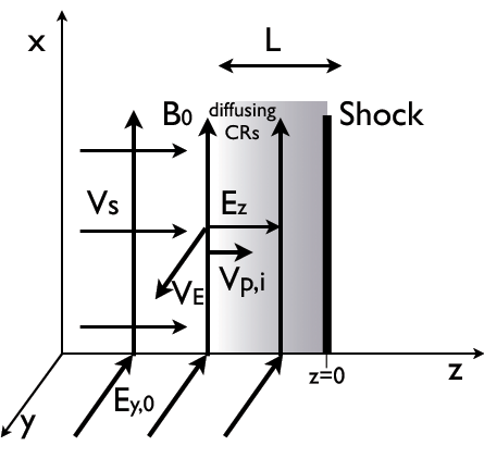
Figure 1: Plasma flows in he frame of the shock. Far upstream, the incoming plasma moves with velocity $v_{s}$, magnetic field is along $x$ direction and inductive electric field along $-y$ direction. At the shock, cosmic rays are accelerated and diffuse ahead of the shock a typical distance $L$, creating an electric field along the shock normal. Electric drift of cosmic rays in this induced electric field  and the initial magnetic field  produces $z$-dependent electric drift $v_{E}$ in $y$ direction. Acceleration of plasma in $y$ direction in turn produces polarization drift of ions in $z$ direction.

III Drift motions in non-neutral plasma

III.1 General relations

Let us consider stationary plasma motion in the frame of the shock. Let ion, electron velocities, magnetic and electric fields be given by

$${\bf v}_{i}=\{0,v_{i,y},v_{i,z}\}\mbox{}$$

$${\bf v}_{e}=\{0,v_{e,y},v_{e,z}\}\mbox{}$$

$${\bf E}=\{0,-E_{y,0},E_{z}\}\mbox{}$$

$${\bf B}=\{B_{x},0,0\}$$ (13)

($E_{y,0}$ is constant because ${\rm curl}{\bf E}=0$). Assuming massless electrons and massive ions, equations of motion are

$${\bf E}+{{\bf v}_{e}\over c}\times{\bf B}=0\mbox{}$$

$$({\bf v}_{i}\nabla){\bf v}_{i}={e\over m_{i}}\left({\bf E}+{{\bf v}_{i}\over c}\times{\bf B}\right)$$ (14)

Maxwell’s equations and continuity require

$${\rm curl}{\bf B}={4\pi e\over c}\left(n_{i}{\bf v}_{i}+n_{cr}\left({E_{z}\over B_{x}}c\right){\bf e}_{y}-n_{e}{\bf v}_{e}\right)\mbox{}$$

$${\rm\,div}{\bf E}=4\pi e(n_{i}+n_{cr}-n_{e})\mbox{}$$

$$n_{i}v_{i,z}=n_{0,ISM}v_{s}=n_{e}v_{e,z}$$ (15)

Cosmic rays experience just the electric drift along $y$ direction due to combined electric field of cosmic rays and plasma particles.

Eliminating electron’s velocities from Eq. (14)

$$v_{e,z}={E_{y,0}\over B_{x}}c\mbox{}$$

$$v_{e,y}={E_{z}\over B_{x}}c$$ (16)

we get four equations for $v_{i,y},v_{i,z},B_{x},E_{z}$:

$$v_{i,z}v_{i,y}^{\prime}={e\over m_{i}}\left(-E_{y,0}+{v_{i,z}\over c}B_{x}\right)\mbox{}$$

$$v_{i,z}v_{i,z}^{\prime}={e\over m_{i}}\left(E_{z}-{v_{i,y}\over c}B_{x}\right)\mbox{}$$

$$E_{z}^{\prime}=4\pi e\left(n_{0,ISM}v_{s}\left({1\over v_{i,z}}-{B_{x}\over cE_{y,0}}\right)+n_{cr}\right)\mbox{}$$

$$B_{x}^{\prime}={4\pi e\over c}\left(n_{0,ISM}v_{s}\left({v_{i,y}\over v_{i,z}}-{E_{z}\over E_{y,0}}\right)+n_{cr}{E_{z}\over B_{x}}c\right)$$ (17)

III.2 Zero inertia limit

In this limit we assume that $m_{i}\rightarrow 0$. This limit is typically not applicable to astrophysical plasmas, since it implies that $\omega_{p,i}/\omega_{B,i}\rightarrow 0$, while, in fact, an opposite limit, $\omega_{p,i}/\omega_{B,i}\gg 1$ is relevant. Still, the limit of massless protons allows an exact treatment and highlights a number of important details. A somewhat different approach to this problem in given in Appendix A.

In the massless limit, $m_{i}\rightarrow 0$, we find

$$v_{i,y}={E_{z}\over E_{y,0}}v_{i,z}\mbox{}$$

$$B_{x}={cE_{y,0}\over v_{i,z}}$$ (18)

which gives

$$B_{x}^{\prime}={4\pi en_{cr}E_{z}\over B_{x}}\mbox{}$$

$$E_{z}^{\prime}={4\pi en_{cr}}$$ (19)

For a given distribution of cosmic rays, of the form $n_{cr}=n_{0,cr}e^{z/L}$, we find

$$v_{i,z}={1\over\sqrt{1+(L/r_{B}(z))^{2}}}v_{s}\mbox{}$$

$$v_{i,y}={L/r_{B}(z)\over\sqrt{1+(L/r_{B}(z))^{2}}}c\mbox{}$$

$$B_{x}=B_{0}\sqrt{1+(L/r_{B}(z))^{2}}\mbox{}$$

$$n_{i}=n_{0,ISM}\sqrt{1+(L/r_{B}(z))^{2}}E_{z}={L\over r_{B}(z)}B_{0}$$ (20)

where

$$r_{B}={B\over 4\pi n_{0,cr}e}$$ (21)

is the so-called magnetic Debye radius associated with cosmic rays. (The statement in Gordeev06 that in non-neutral plasmas the magnetic field is screened on the magnetic Debye radius $r_{B}$ is incorrect). Thus, if $L\sim r_{B}(0)$, the electromagnetic drift can become relativistic.

Note that magnetic field in the plasma rest frame $B^{\prime}=B_{z}/\Gamma$, where $\Gamma=1/\sqrt{1-(v_{y}^{2}+v_{z}^{2})/c^{2}}$ remains constant, $B^{\prime}=B_{0}\sqrt{1-(v_{s}/c)^{2}}$ (it would have been more correct to use $B^{\prime}$ instead of $B_{0}$ as a parameter of the problem).

For a typical ISM plasma

$$r_{B}\approx 10^{3}{\rm cm}{1\over\xi_{cr}}B_{-5}n_{0,ISM}^{-1}$$ (22)

is very small even for small cosmic ray fraction $\xi_{cr}\ll 1$. This highlights the fact that even a small charge disbalance can lead to substantial changes in the upstream region.

III.3 Drift equation with polarization current

In the previous section we showed that charge disbalance ahead of the shock can lead to substantial velocities, and thus requires taking inertial contributions into account. In Eq. (17), eliminating $y$ component of ion velocity

$$v_{i,y}=\left({E_{z}\over B_{x}}-{m_{i}v_{i,z}v_{i,z}^{\prime}\over eB_{x}}\right)c$$ (23)

we find

$$v_{i,z}-v_{s}=\left(b_{x}\partial_{z}E_{z}-\partial_{z}b_{x}E_{z}\right){m_{i}c^{2}v_{i,z}\over eB_{0}^{2}b_{x}^{2}}-\left((\partial_{z}v_{i,z})^{2}+v_{i,z}\partial^{2}_{z}v_{i,z}-v_{i,z}\partial_{z}v_{i,z}\partial_{z}b_{x}\right){m_{i}^{2}c^{2}v_{i,z}\over e^{2}B_{0}^{2}b_{x}^{2}}\mbox{}$$

$$\partial_{z}b_{x}={4\pi\over B_{0}^{2}b_{x}}\left(E_{z}\left(n_{0}({v_{s}\over v_{i,z}}-b_{x})+n_{cr}\right)-{m_{i}n_{0}v_{s}\partial_{z}v_{i,z}}\right)\mbox{}$$

$$\partial_{z}E_{z}={4\pi e}\left(n_{0}({v_{s}\over v_{i,z}}-b_{x})+n_{cr}\right)$$ (24)

where we introduced $b_{x}=B_{x}/B_{0}$.

The drift approximation corresponds to expansion in $1/e$, one over electric charge Kulsrud . In a non-neutral plasma it is important to keep two leading expansion orders:

$$v_{i,z}-v_{s}=\left(b_{x}\partial_{z}E_{z}-\partial_{z}b_{x}E_{z}\right){m_{i}c^{2}v_{i,z}\over eB_{0}^{2}b_{x}^{2}}\mbox{}$$

$$\partial_{z}b_{x}={4\pi\over B_{0}^{2}b_{x}}\left(E_{z}\left(n_{0}({v_{s}\over v_{i,z}}-b_{x})+n_{cr}\right)-{m_{i}n_{0}v_{s}\partial_{z}v_{i,z}}\right)\mbox{}$$

$$\partial_{z}E_{z}={4\pi e}\left(n_{0}({v_{s}\over v_{i,z}}-b_{x})+n_{cr}\right)$$ (25)

To proceed further, we assume that the polarization drift is weak, and expand in small quantities $v_{i,z}-v_{s}$, $b_{x}-1$, $n_{cr}$ and $E_{z}$.

$$v_{i,z}-v_{s}=-v_{s}(b_{x}-1)+{m_{i}c^{2}v_{s}\over B_{0}^{2}e}\partial_{z}E_{z}\mbox{}$$

$$\partial_{z}b_{x}=-{4\pi m_{i}n_{0,ISM}\over B_{0}^{2}}\partial_{z}v_{i,z}\mbox{}$$

$$\partial_{z}E_{z}=4\pi e\left(n_{0}({v_{i,z}-v_{s}\over v_{s}}-b_{x})+n_{cr}\right)$$ (26)

Which immediately gives

$${v_{i,z}-v_{s}\over v_{s}}=-M_{A}^{-2}(b_{x}-1)$$ (27)

where $M_{A}=v_{s}/v_{A}$. The solutions for the electromagnetic fields and components’ velocities are

$$b_{x}=1+{\xi_{cr}(z)\over(1+\beta_{A}^{2})(1-1/M_{A}^{2})}\approx 1+\xi_{cr}(z)\mbox{}$$

$$E_{z}={L\omega_{B,i}\over c}{\xi_{cr}(z)\over 1+\beta_{A}^{2}}B_{0}\approx{L\omega_{B,i}\over c}{\xi_{cr}(z)}B_{0}\mbox{}$$

$$v_{e,y}=L\omega_{B,i}{\xi_{cr}(z)\over 1+\beta_{A}^{2}}\approx L\omega_{B,i}\xi_{cr}(z)\mbox{}$$

$$v_{e,z}=v_{s}\left(1-{\xi_{cr}(z)\over(1+\beta_{A}^{2})(1-1/M_{A}^{2})}\right)\approx v_{s}(1-\xi_{cr}(z))\mbox{}$$

$$v_{i,y}={\omega_{B,i}c^{2}\over L\omega_{p,i}^{2}}{1+(L\omega_{p,i}/c)^{2}(1-1/M_{A}^{2})\over(1+\beta_{A}^{2})(1-1/M_{A}^{2})}\approx L\omega_{B,i}\left(1+{c^{2}\over\omega_{p,i}^{2}L^{2}}\right)\xi_{cr}(z)\mbox{}$$

$$n_{e}=n_{0,ISM}\left(1+{\xi_{cr}(z)\over(1-1/M_{A}^{2})(1+\beta_{A}^{2})}\right)\mbox{}$$

$$n_{i}=n_{0,ISM}\left(1+{\xi_{cr}(z)\over(M_{A}^{2}+1)(1+\beta_{A}^{2})}\right)\mbox{}$$

$$n_{i}-n_{e}=-{n_{cr}\over 1+\beta_{A}^{2}}\mbox{}$$

$$n_{tot}={\beta_{A}^{2}\over 1+\beta_{A}^{2}}n_{cr}\approx\beta_{A}^{2}n_{cr}\ll n_{cr}$$ (28)

where $\beta_{A}=(\omega_{B,i}/\omega_{p,i})$. (Relations (28) assume a specific cosmic ray density distribution, $\xi_{cr}(z)=\xi_{cr,0}e^{z/L}$.) Equations (28) solve a problem of modification of the upstream plasma in perpendicular shocks by cosmic rays diffusing ahead of the shock.

The electric drift velocity is typically much smaller than the shock velocity. If we introduce parameter $\eta$ as cosmic ray acceleration efficiency,

$$\eta={\gamma n_{cr}m_{i}c^{2}\over m_{i}n_{0,ISM}v_{s}^{2}/2},$$ (29)

then with partial screening of the cosmic ray-induced electric field by the incoming plasma, the transverse velocity of the incoming plasma,

$$v_{E}\sim\xi_{cr}c^{2}/v_{s}\approx v_{s}{\eta\over 2}v_{s}$$ (30)

is typically smaller than the shock velocity.

IV Instabilities

IV.1 Fluid instabilities in upstream plasma

There is a number of instabilities that can operate in the upstream plasma. First, there are fluid instabilities that may develop in the sheared flow in the upstream medium: Kelvin Helmholtz (KH) instability of ideal flows and viscously-driven instabilities of flows with high Reynolds numbers. KH instability of sheared flows requires inflection point in the velocity profile (Rayleigh condition). This cannot be achieved in the present model, where diffusion coefficient was assumed to constant, so that electric drift velocity is proportional to smoothly decreasing density of cosmic rays, Eq. (28). On the other hand, if diffusion has a more complicated spacial dependence (e.g. it is higher closer to the shock, where the level of turbulence is higher, one might expect an inflection point.

Allowing for spacial variation of the diffusion coefficient, the cosmic ray number density becomes

$$\partial_{z}^{2}n={v-\partial_{z}\kappa\over\kappa}\partial_{z}n$$ (31)

Thus, if the diffusion changes on scale $L\sim v/\kappa$, one may have an inflection point in the flow. (Note that since diffusion is lower far away from a shock, $\partial_{z}\kappa>0$.) For example, if the diffusion coefficient has a dependence $\kappa=\kappa_{0}e^{z/L}$, the inflection point occurs at $z=-L\ln(\kappa_{0}/(Lv_{s}))$. Eq. (28) then indicates that the electric drift velocity will also have an inflection point, resulting in KH instability.

IV.2 Electromagnetic instabilities: modified Buneman

In addition to fluid instabilities, plasmas with ”real” drift of particles (as opposed, e.g. to effective Larmor drift in inhomogeneous plasma), is subject to a number of powerful instabilities, related, generally speaking to Buneman current instability, and in particular to the so called modified Buneman instability (1962JNuE….4..111B, ).

In keeping with our approach, we next consider hydrodynamic-type (non-kinetic) instability driven by a perpendicular ion current. Since the modified Buneman instability is of the mixed electrostatic-electromagnetic type, it is necessary to keep electron inertia. Let us transform to a frame which is drifting with velocity $v_{E}$ along the shock normal and is advected with shock velocity $v_{s}$. In this frame the ions are drifting with respect to electrons with the polarization drift velocity $v_{p}\sim\xi_{cr}v_{s}$ directed along $z$ axis. In considering stability of such plasma, we neglect small variations of the magnetic field and associated current along $y$ direction, as well as related variations of electron and ion densities.

Since the electrostatic contributions to the dielectric tensor are most important, we chose wave vector of perturbations along $z$ direction, ${\bf k}=k_{z}{\bf e}_{z}$. Let the fluctuating part of the vector potential (in radiation gauge) ${\bf A}$ be ${\bf A}=a_{y}{\bf e}_{y}+a_{z}{\bf e}_{z}$. The fluctuating electric and magnetic fields are $\delta{\bf E}=i(\omega/c)\{0,a_{y},a_{z}\}$, $\delta{\bf B}=-ik_{z}\{a_{y},0,0\}$. Introducing electron and ion displacements ${\bf\xi}_{e}=\{\xi_{e,x},\xi_{e,y},\xi_{e,z}\}$ and ${\bf\xi}_{i}=\{\xi_{i,x},\xi_{i,y},\xi_{i,z}\}$, the equations of motions for electrons and ions are

$$\partial_{t}{{\bf v}}_{e}+({\bf v}_{e}\cdot\nabla){\bf v}_{e}=-{e\over m_{e}}\left({\bf E}+{{\bf v}}_{e}\times{\bf B}\right)\mbox{}$$

$$\partial_{t}{{\bf v}}_{i}+({\bf v}_{i}\cdot\nabla){\bf v}_{i}={e\over m_{i}}\left({\bf E}+{{\bf v}}_{i}\times{\bf B}\right)\mbox{}$$

$${\bf v}_{i}=v_{p}{\bf e}_{z}+\partial_{t}{\bf\xi}_{i}\mbox{}$$

$${\bf v}_{e}=\partial_{t}{\bf\xi}_{e}$$ (32)

Electromagnetic fields are related by

$$\partial_{t}{{\bf B}}=-\nabla\times{\bf E}\mbox{}$$

$$\partial_{t}{\bf E}=\nabla\times{\bf B}-{4\pi\over c}\left(n_{i}{\bf v}_{i}-n_{e}{\bf v}_{e}\right)$$ (33)

Finally, continuity equations give

$$\partial_{t}n_{e}+\nabla(n_{e}{{\bf v}}_{e})=0\mbox{}$$

$$\partial_{t}n_{i}+\nabla(n_{i}{{\bf v}}_{i})=0$$ (34)

We find

$$\xi_{e,x}=\xi_{i,x}=0\mbox{}$$

$$\xi_{e,y}={e\over m_{e}c}{1\over\omega^{2}-\omega_{B,e}^{2}}\left(i\omega a_{y}+\omega_{B,e}a_{z}\right)\mbox{}$$

$$\xi_{e,z}={e\over m_{e}c}{1\over\omega^{2}-\omega_{B,e}^{2}}\left(\omega_{B,e}a_{y}-i\omega a_{z}\right)\mbox{}$$

$$\xi_{i,y}={e\over cm_{i}\omega}{1\over\tilde{\omega}^{2}-\omega_{B,i}^{2}}\left(-i\tilde{\omega}^{2}a_{y}+\omega_{B,i}\omega a_{z}\right)\mbox{}$$

$$\xi_{i,z}=-{e\over cm_{i}\omega}{\tilde{\omega}\over\tilde{\omega}^{2}-\omega_{B,i}^{2}}\left(\omega_{B,i}a_{y}+i\omega a_{z}\right)\mbox{}$$

$$\tilde{\omega}=\omega-k_{z}v_{p}\mbox{}$$

$$n_{e}=n_{0}\left(1-ik_{z}\xi_{e,z}\right)\mbox{}$$

$$n_{i}=n_{0}\left(1-i{k_{z}\omega\xi_{i,z}\over\tilde{\omega}}\right)$$ (35)

which gives the equation for normal modes

$$\left(\begin{array}[]{cc}n^{2}-1+S_{e}+{\tilde{\omega}^{2}\over\omega^{2}}S_{i}&iD\\ -iD&-1+S_{e}+S_{i}\end{array}\right)\left(\begin{array}[]{c}a_{y}\\ a_{z}\end{array}\right)=0$$ (36)

where

$$S_{e}={\omega_{p,e}^{2}\over\omega^{2}-\omega_{B,e}^{2}}\mbox{}$$

$$S_{i}={\omega_{p,i}^{2}\over\tilde{\omega}^{2}-\omega_{B,e}^{2}}\mbox{}$$

$$D=-{\omega_{B,e}\over\omega}S_{e}+{\omega_{B,i}\over\omega}S_{i}$$ (37)

The dispersion relation follows from (36):

$$n^{2}=1-S_{e}-{\tilde{\omega}^{2}\over\omega^{2}}S_{i}-{D^{2}\over 1-S_{e}-S_{i}}$$ (38)

The eigenmodes satisfy

$$a_{y}=i{1-S_{e}-S_{i}\over D}a_{z}$$ (39)

Thus, the eigenmodes are elliptically polarized. Note, that the wave vector of the perturbations lies in the polarization plane, so that the wave is of a mixed electrostatic-electromagnetic type.

For vanishing drift velocity, $v_{p}=0$, in the low frequency limit $\omega_{B,e}\rightarrow\infty$, Eq. (36) gives the extraordinary mode

$$n^{2}=1-S_{e}-S_{i}-{D^{2}\over 1-S_{e}-S_{i}}=1+{(\omega_{p,i}^{2}+\omega_{B,i}^{2})\omega_{p,i}^{2}\over\omega_{B,i}^{2}(\omega_{p,i}^{2}+\omega_{B,i}^{2}-\omega^{2})}\approx\omega_{p,i}^{2}/\omega_{B,i}^{2}$$ (40)

In case of finite drift velocity, keeping terms linear in $m_{e}/m_{i}$ and assuming $\tilde{\omega}\ll\omega_{B,i}$, we find

$$n^{2}=1+\left({m_{e}\over m_{i}}+{\tilde{\omega}^{2}\over\omega^{2}}\right){\omega_{p,i}^{2}\over\omega_{B,i}^{2}}$$ (41)

which gives

$$\omega\approx k_{z}\left(v_{p}\pm\sqrt{v_{A}^{2}-v_{p}^{2}(m_{e}/m_{i}+\beta_{A}^{2})}\right)$$ (42)

Equation (41) has complex roots provided

$$v_{p}>{v_{A}\over\sqrt{(m_{e}/m_{i})+\beta_{A}^{2}}}$$ (43)

If $\beta_{A}\ll\sqrt{m_{e}/m_{i}}$ (this requires $B<7\times 10^{-5}{\rm G}\,n_{0,ISM}^{1/2}$), the instability occurs for

$$v_{p}>\sqrt{m_{i}/m_{e}}v_{A}$$ (44)

Since polarization drifts velocity is $v_{p}\sim\xi_{cr}v_{s}$, it is required for instability that

$$\xi_{cr}>\sqrt{m_{i}\over m_{e}}{1\over M_{A}}$$ (45)

where $M_{A}=v_{s}/v_{A}\gg 1$ is the shock Mach number.

For velocities larger than (44), the instability growth rate is

$$\Gamma=\sqrt{m_{e}\over m_{i}}\xi_{cr}k_{z}v_{s}$$ (46)

The instability has time to grow $\sim L/v_{s}$; the requirement $\Gamma L/v_{s}>1$ limits the wave number of growing modes to

$$2\sqrt{m_{i}/m_{e}}{1\over M_{A}\eta}<k_{z}\delta_{i}<1$$ (47)

where $\delta=c/\omega_{p,i}$ is ion skin depth. The upper limit on $k_{z}<1/\delta_{i}$ follows from neglect of kinetic effects.

Thus, if cosmic ray acceleration efficiency is

$$\eta>2\sqrt{m_{i}\over m_{e}}{1\over M_{A}}$$ (48)

instability will have enough time to grow. Condition (48) favors strong shocks with weak magnetic field.

What is the nature of the unstable modes? Eq. (42) indicates that both eigenmodes become unstable, implying that both components of the electric fields orthogonal to the initial magnetic field, as well as fluctuations of magnetic field along the initial magnetic field, grow exponentially. Eq. (39) indicates that the phases of the electric field components $E_{z}$ and $E_{y}$ are shifted by ninety degrees, implying that growing modes correspond to vortical perturbations. These kinds of perturbations will shuffle field line along $z$ direction. If we allow for finite perturbations along $x$ and $y$ direction, the instability will induce field line wandering. Since field line wandering can bring both signs of charge, this might be break down our assumption of charge non-neutral plasma. Still, the motion of electrons and ions along the field line might proceed in different regime: resulting magnetic field amplification and corresponding magnetic bottles will reflect electrons more efficiently due to their small Larmor radius.

IV.3 Applicability and saturation

The applicability of our approach requires that (i) the diffusion length $L$ is larger than the Larmor radius of cosmic rays  $r_{L,cr}=\gamma c/\omega_{B,i}$ – this condition is satisfied for any non-relativistic shock, since $L\sim(c/v_{s})r_{L,cr}\gg r_{L,cr}$; (ii) $L$ is larger than skin-depth of cosmic ray component, $\delta_{cr}=c/\omega_{p,cr}$. We find

$${L\over\delta_{cr}}=\sqrt{\gamma\xi_{cr}}{c\over v_{s}}{c\over v_{A}}=\sqrt{\eta\over 2}{c\over v_{A}}$$ (49)

This puts a lower limit on cosmic ray efficiency

$$\eta>2(\beta_{A})^{2}=10^{-10}{1\over n_{ISM}}{B_{-6}}^{2}$$ (50)

which can be easily satisfied.

The growth rate (46) was calculated assuming cold ions and electrons. This is justified if the polarization drift velocity is larger than electrons thermal speed $v_{T,e}$, $v_{p}=\xi_{cr}v_{s}>\sqrt{T/m_{e}}$. This requires

$$\xi_{cr}>\sqrt{m_{i}\over m_{e}}{1\over M_{s}}$$ (51)

where $M_{s}=v_{s}/v_{T,i}$ is the conventional Mach number. The condition (51) is quite restrictive, so that the modified Buneman instability may also heat electrons. Previously, it was suggested 2007ApJ…654L..69G ; 2008ApJ…684..348R that lower hybrid waves in the CR precursor of a perpendicular shock might be a plausible electron heating mechanism. To assess the efficiency of electron heating, kinetic-type calculations are required; we postpone them to a future paper. For drift velocities smaller than ion thermal speed, ${\bf v}_{p}\leq v_{T,i}$ it is expected that the instability will be stabilized. This requirement places a lower limit on cosmic ray faction, $\xi_{cr}>1/M_{A}$.

To estimate the saturation level of instability, we assume that a large fraction of the ion polarization drift is converted into fluctuating magnetic field. This gives an estimate

$$\left({\delta B\over B_{0}}\right)^{2}\sim M_{A}^{2}\xi_{cr}^{3}\geq{1\over M_{A}}$$ (52)

V Discussion

We considered how cosmic ray accelerated at perpendicular shocks and diffusing kinetically ahead of the shock modify the upstream flow. First, the electric charge density induced by cosmic ray diffusion is mostly, but not completely, screened by the polarization drift in the upstream plasma. The remaining charge density induces shear along the shock plane, so that the shock become oblique (in a sense that the flow velocity is not aligned with the shock normal; magnetic field remains orthogonal to the shock normal).

For fast shocks with high efficiency of cosmic ray acceleration (so that the condition (45) is satisfied), modified Buneman instability develops. In addition, a sheared flow can be unstable to fluid shearing instabilities. Both fluid and drift current instabilities would generate turbulence and presumably enhanced particle diffusion, vindicating the assumption that perpendicular shocks are efficient cosmic ray accelerators. The proposed instability can also be important for electron heating in the cosmic ray precursor. This requires a kinetic treatment of the instability. In addition, since the higher energy particles are diffusing faster, the resulting population inversion ahead of the shock may drive cyclotron instabilities; we leave consideration of this possibility to a future paper.

In case of parallel shocks, development of Bell’s instability leads to generation of fluctuating perpendicular magnetic fields, which become dominant over the initial parallel field 2008ApJ…682L…5S . In that case, the instability discussed in this paper can be regarded as a secondary instability of the cosmic ray-modified parallel shocks.

The effect discussed in this paper is due to non-neutrality of the upstream plasma and thus is easily missed in a conventional MHD treatment. In addition, we assume that kinetic cosmic ray diffusion dominates over field line wandering, at least upstream of the shock. If particle were to diffuse mostly by field line wandering, charge neutrality would be established by drawing a parallel current. Also, we did not address the issues of particle injections, i.e., how to start the process going.

I would like to thank Elena Amato, Benjamin Chandran, Martin Laming and Anatoly Spitkovsky for the most enlightening discussions.

Appendix A Magnetic field in the upstream plasma

In this Appendix we re-derive behavior of magnetic field ahead of the shock neglecting inertial effects. Let us assume that a flow carrying magnetic field $B_{0}$ approaches a perpendicular shock, and that due to the acceleration of cosmic ray particles there is a layer of uncompensated charge in front of the shock. Neglecting diamagnetic currents induced by cosmic rays as well as pressure of cosmic rays, the equation of motion of cosmic rays  and electromagnetic fields reduces to

$${\bf E}+{{\bf v}\over c}\times{\bf B}=0$$ (53)

here ${\bf E}$ and ${\bf v}$ are total electric fields and drift velocities. Let the density within the charged layer be $n_{tot}$ and the thickness of the layer be $L$. Since the charge-separated current is ${\bf j}=en_{tot}{\bf v}$, and $\nabla\times{\bf B}=(4\pi/c){\bf j}$, we find

$${\bf E}+{1\over 4\pi en_{tot}}\nabla\times{\bf B}\times{\bf B}=0$$ (54)

Taking divergence of this equation gives

$$n_{tot}+{c^{2}\over 16\pi^{2}e^{2}}\nabla\cdot\left({\nabla\times{\bf B}\over n_{tot}}\times{\bf B}\right)=0$$ (55)

The Eq. (55) reminds of the plasma dynamics in the limit of electron MHD [10]. For given $n_{tot}$ and $L$, the modification of magnetic field depends only on number density of cosmic rays, Eq. (55), and not on their energy.

Eq. (55) can be integrated,

$$B_{x}^{2}={16\pi^{2}e^{2}\over c^{2}}{{\cal N}^{2}}+C_{1}{\cal N}+C_{0}\mbox{}$$

$${\cal{N}}(z)=\int_{z}^{0}n_{tot}(z)dz$$ (56)

where $C_{1}$ and $C_{0}$ are integration constants. The quantity ${\cal N}(z)$ is a surface density of cosmic rays ahead of the shock, integral of density from a given position $z$ up to the shock front. (Recall that in the zero inertia limit there is no compensating polarization drift of bulk ions.) In the particular case when the density of cosmic rays is given by Eq. (2), ${\cal N}(z)=n_{0,cr}L(1-e^{z/L})$, so that ${\cal N}(z=-\infty)=n_{0,cr}L$. Since the magnetic field at $z=-\infty$ is $B_{0}$, this gives

$$B_{0}^{2}={16\pi^{2}e^{2}n_{0,cr}L\over c^{2}}+C_{1}n_{0,cr}L+C_{0}$$ (57)

Assuming assume that $z$-component of the electric field is zero and magnetic field is $B_{0}$ at $z=-\infty$, we find

$$B_{x}^{2}=B_{0}^{2}\left(1+{L^{2}\over r_{B}(z)^{2}}\right)\mbox{}$$

$$E_{z}={L\over r_{B}(z)}B_{0}$$ (58)

Consistent with Eq. (20). Again, the apparent increase of magnetic field is, in fact, due to the Lorentz boost along $y$ direction with electric drift velocity

$${v_{E}\over c}={L/r_{B}(z)\over\sqrt{1+L^{2}/r_{B}(z)^{2}}}$$ (59)

References

- [1] W. I. Axford, E. Leer, and J. F. McKenzie. The structure of cosmic ray shocks. AAP, 111:317–325, July 1982.
- [2] A. R. Bell. Turbulent amplification of magnetic field and diffusive shock acceleration of cosmic rays. MNRAS, 353:550–558, September 2004.
- [3] R. Blandford and D. Eichler. Particle acceleration at astrophysical shocks: A theory of cosmic ray origin. Phys. Rep., 154:1–75, October 1987.
- [4] O. Buneman. Instability of electrons drifting through ions across a magnetic field. Journal of Nuclear Energy, 4:111–117, January 1962.
- [5] A. A. Galeev. Generation of ultrarelativistic electrons by shock waves and the associated synchrotron emission. Zhurnal Eksperimental noi i Teoreticheskoi Fiziki, 86:1655–1666, May 1984.
- [6] M. Gedalin. Ion reflection at the shock front revisited. J. Geoph. Res., 101:4871–4878, March 1996.
- [7] P. Ghavamian, J. M. Laming, and C. E. Rakowski. A Physical Relationship between Electron-Proton Temperature Equilibration and Mach Number in Fast Collisionless Shocks. ApJ Lett., 654:L69–L72, January 2007.
- [8] J. Giacalone and J. R. Jokipii. The Transport of Cosmic Rays across a Turbulent Magnetic Field. Astrophys. J. , 520:204–214, July 1999.
- [9] A. V. Gordeev. Formation of nonquasineutral vortex plasma structures with a zero net current. Plasma Physics Reports, 32:921–926, November 2006.
- [10] A. S. Kingsep, K. V. Chukbar, and V. V. Ian’kov. Electron magnetohydrodynamics. Voprosy Teorii Plazmy, 16:209–250, 1987.
- [11] R. M. Kulsrud. Plasma physics for astrophysics. 2005.
- [12] W. H. Matthaeus, G. Qin, J. W. Bieber, and G. P. Zank. Nonlinear Collisionless Perpendicular Diffusion of Charged Particles. ApJ Lett., 590:L53–L56, June 2003.
- [13] K. G. McClements, R. O. Dendy, R. Bingham, J. G. Kirk, and L. O. Drury. Acceleration of cosmic ray electrons by ion-excited waves at quasi-perpendicular shocks. MNRAS, 291:241–249, October 1997.
- [14] K. Papadopoulos. Electron heating in superhigh Mach number shocks. Astroph. Space Sci., 144:535–547, May 1988.
- [15] C. E. Rakowski, J. M. Laming, and P. Ghavamian. The Heating of Thermal Electrons in Fast Collisionless Shocks: The Integral Role of Cosmic Rays. Astrophys. J. , 684:348–357, September 2008.
- [16] A. Spitkovsky. Particle Acceleration in Relativistic Collisionless Shocks: Fermi Process at Last? ApJ Lett., 682:L5–L8, July 2008.
- [17] O. L. Vaisberg, A. A. Galeev, G. N. Zastenker, S. I. Klimov, M. N. Nozdrachev, R. Z. Sagdeev, A. I. Sokolov, and V. D. Shapiro. Electron acceleration at the front of strong collisionless shock waves. Zhurnal Eksperimental noi i Teoreticheskoi Fiziki, 85:1232–1243, October 1983.