On a Model for Mass Aggregation with Maximal Size

Abstract

We study a kinetic mean-field equation for a system of particles with different sizes, in which particles are allowed to coagulate only if their sizes sum up to a prescribed time-dependent value. We prove well-posedness of this model, study the existence of self-similar solutions, and analyze the large-time behavior mostly by numerical simulations. Depending on the parameter $k_{0}$, which controls the probability of coagulation, we observe two different scenarios: For $k_{0}>2$ there exist two self-similar solutions to the mean field equation, of which one is unstable. In numerical simulations we observe that for all initial data the rescaled solutions converge to the stable self-similar solution. For $k_{0}<2$, however, no self-similar behavior occurs as the solutions converge in the original variables to a limit that depends strongly on the initial data. We prove rigorously a corresponding statement for $k_{0}\in(0,1/3)$. Simulations for the cross-over case $k_{0}=2$ are not completely conclusive, but indicate that, depending on the initial data, part of the mass evolves in a self-similar fashion whereas another part of the mass remains in the small particles.

Keywords:

aggregation with maximal size, self-similar solutions,
coarsening in coagulation models

MSC (2000):

45K05, 82C22

1 Introduction

Mass aggregation is a fundamental process that appears in a large range of applications, such as formation of aerosols, polymerization, clustering of stars or ballistic aggregation, see for instance [2, 6, 12]. In all these applications, certain types of ’particles’ form clusters that are characterized by their ’size’ or ’mass’ $x$. Smoluchowski’s [11] classical mesoscopic mean-field description of irreversible aggregation processes describes the evolution of the number density $g(t,x)$ of clusters of size $x$ per unit volume at time $t$. Clusters of size $x$ and $y$ can coalesce by binary collisions to form clusters of size $x+y$ at a rate given by a kernel $K(x,y)$, such that the dynamics of $g$ is given by

$$\frac{\partial}{\partial t}g(t,x)=\frac{1}{2}\int_{0}^{x}K(y,x-y)g(t,x-y)g(t,y)\,dy\,-\,g(t,x)\int_{0}^{\infty}K(x,y)g(t,y)\,dy\,.$$ (1)

An issue of fundamental interest in the mathematical analysis of coagulation processes is the phenomenon of dynamic scaling for homogeneous kernels. This means that for initial data from a certain class the solution to (1) converges to a certain self-similar solution. Unfortunately, except for some special kernels such as the constant one, this question is still only poorly understood (see e.g. [8] for an overview). While it has been common belief in the applied literature that self-similar solutions are unique, it has recently been shown for some special kernels [9] that there is a whole one-parameter family of self-similar solutions. These solutions can be distinguished by their tail behavior, and their respective domains of attraction are characterized by the tail behavior of the initial data.

In contrast to this, very little is known for other homogeneous kernels. The existence of fast-decaying self-similar solutions for a range of kernels is established in [3, 4], but both the existence of solutions with algebraic tail and the uniqueness of solutions are still open problems. In general, unless explicit methods such as the Laplace transform work, just proving existence of self-similar solutions to a coagulation equation can be a formidable task.

Thus, despite their fundamental role, many properties of mean-field models for coagulation processes, in particular with respect to dynamic scaling, are not well understood. Motivated by an application of elasto-capillary coalescence of wetted polyester lamellas [1], we investigate this question for a special singular coagulation kernel $K$. This kernel allows only those clusters to coagulate that can form clusters of a given maximal size. To our knowledge this is the first mathematical analysis for such type of kernels. Even though tails of the size distribution do not play a role here, we find that self-similar solutions are still not unique and the analysis of the long-time behavior turns out to be delicate.

In model considered here, two particles can coagulate only if the sum of their sizes is equal to $M(t)$, where $M$ is a given increasing function of time. This means that at time $t$ only particles of size $M(t)$ are emerging and the amount of particles of all smaller sizes is decreasing. This corresponds to $K(x,y,t)\sim\delta_{0}(x+y-M(t))$, where $\delta_{0}$ denotes the delta-distribution in $0$ and the factor of proportionality may depend on time.

As above, we denote the number density of particles of size $x$ at time $t$ by $g(t,x)$. The total number of particles per unit volume at time $t$ is then $N(t)=\int_{0}^{M(t)}g(t,x)dx$. At time $t$, the density of particles of any size $x<M(t)$ is decreasing at a rate proportional to the probability density of a particle of size $x$ meeting a particle of size $M(t)-x$. The coagulation process can hence be described by

$$\frac{\partial g}{\partial t}(t,x)=-K(t)\frac{g(t,x)}{N(t)}\frac{g(t,M(t)-x)}{N(t)}$$

where $K(t)$ is a rate function proportional to the expected number of coagulation events per unit time. Motivated by [1] we make the ansatz $K(t)=k_{0}M^{\prime}(t)N(t)$, where $k_{0}$ is a constant of proportionality that depends on the particular physical process. The above equation hence reads

$$\frac{\partial g}{\partial t}(t,x)=-\frac{k_{0}M^{\prime}(t)}{N(t)}g(t,x)g(t,M(t)-x).$$ (2)

The coagulation process described above neither creates nor destroys mass, which is expressed by the mass conservation equation

$$\int_{0}^{M(t)}xg(t,x)dx=\sigma$$ (3)

where $\sigma$ is a constant. From (2) and (3) we will derive an equivalent condition for $g(t,M(t))$, see Equation (7) below.

For $x>M(t)$, $g(t,x)$ is not changing since particles of size greater than $M(t)$ can not form a particle of size $M(t)$ by coagulation. Hence $\frac{\partial g}{\partial t}(t,x)=0$ for $x>M(t)$. We are normally interested in processes where the value of $M$ at the starting time is greater than the size of all particles existing initially, and hence we also assume $g(t,x)=0$ for $x>M(t)$.

An important feature of Equation (2) is its invariance under reparametrization of time. As a consequence $M(t)$ is not determined by the initial data but can be prescribed to be an arbitrary increasing function of time (see also [7, 10], where such an invariance has been crucial in the analysis of a model for min-driven clustering). In the following we choose $M(t)=t$ and also normalize the mass by setting $\sigma=1$. Consequently, in what follows we study the system of equations

$$\frac{\partial{g}}{\partial t}(t,x)=-\frac{k_{0}}{N(t)}g(t,x)g(t,t-x),\quad N(t)=\int_{0}^{t}g(t,x)dx,\quad\int_{0}^{t}xg(t,x)dx=1$$ (4)

with $t\geq 1$ and $0\leq{x}\leq{t}$.

The first aim of this article is to establish well-posedness of the initial value problem and to study the long time behavior of solutions to (4). To this end, we prove global existence and uniqueness of mild solutions in Section 2, Theorem 1 by rewriting (4) as a fixed point equation. In contrast to coagulation equations with more regular kernels, for which well-posedness can often be proved in the space of probability measures [5], here we need to work with functions that are continuous up to the points $x=1$ and $x=t$. The reason that the fixed-point argument is not quite straightforward is that at any time there is an influx of particles of the largest size $M(t)$ that leads to a nontrivial boundary condition.

In Section 3 we study the existence of self-similar solutions. Combining rigorous arguments with numerical simulations, we identify $k_{0}=2$ as a critical value: For $k_{0}<2$ no self-similar solutions exist but for $k_{0}>2$ we find two self-similar solutions which have different shape and stability properties. Section 4 is devoted to numerical simulations of initial value problems. Our results for $k_{0}>2$ suggest that, after a suitable rescaling, each solution converges to the second self-similar solution. For $k_{0}<2$, however, $g$ converges to a steady state $g_{\infty}(x)$, $x\in\mathbb{R}^{+}$, whose shape depends strongly on the initial data. We finally prove this assertion in Proposition 6 for $k_{0}<\tfrac{1}{3}$.

2 Global existence and uniqueness of solutions

In this section we derive a notion of mild solutions to (4) that relies on an appropritate reformulation of the mass constraint $\int_{0}^{t}{x}g(t,x)dx=1$. We then use Banachs’s Contraction Mapping Theorem to prove the local existence and uniqueness of mild solutions, and finally employ some a priori estimates to show that these mild solutions exist globally in time.

2.1 Notion of mild solutions and main result

To reformulate the mass constraint (4)₃ we suppose that a piecewise smooth solution $g(t,x)$ to (4)₁ and (4)₂ is given. We then have

$$0 = \frac{d}{dt}\int_{0}^{t}xg(t,x)dx=\int_{0}^{t}x\frac{\partial g}{\partial t}(t,x)dx+tg(t,t),$$ (5)

and due to (4)₁ we obtain

$$tg(t,t)=\frac{k_{0}}{N(t)}\int_{0}^{t}xg(t,x)g(t,t-x)dx.$$ (6)

Moreover, substituting $x\rightsquigarrow{x-t}$ we find

$$\int_{0}^{t}xg(t,x)x(t,t-x)dx = t\int_{0}^{t}g(t,t-x)g(t,x)dx-\int_{0}^{t}xg(t,t-x)g(t,x)dx,$$

so (6) implies

$$g(t,t)=\frac{k_{0}}{2N(t)}\int_{0}^{t}g(t,x)g(t,t-x)dx.$$ (7)

This condition is equivalent to (4)₃ provided that $g(t,x)$ solves (4)₁, and for the ease of notation we introduce the operator $B:g\mapsto{B}[g]$ by

$$B[g](t) := \frac{k_{0}}{2N(t)}\int_{0}^{t}g(t,x)g(t,t-x)dx,$$

where $N$ depends on $g$ via (4)₂.

In what follows we fix some $T>0$ and introduce $X$ as the space of all functions $g$ that satisfy

1. $g:\Omega=[1,T]\times[0,T]\rightarrow\mathbb{R}_{0}^{+}$,

2. $g(1,x)=g_{\mathrm{ini}}(x)$ for all $x\in[0,1]$,

3. $g(t,x)=0$ if $x>t$,

4. $g$ is continuous in all points $(t,x)$ with $x\neq 1$ and $x\neq{t}$,

where the initial data $g_{\mathrm{ini}}$ are supposed to satisfy

$$g_{\mathrm{ini}}\in{C}([0,1];\,\mathbb{R}^{+}),\qquad\int_{0}^{1}x{g_{\mathrm{ini}}(x)}dx=1.$$

To introduce the notion of mild solutions we now define the operator $\Gamma:X\rightarrow X$ by

$$\Gamma[g](t,x)=\left\{\begin{aligned} &g_{\mathrm{ini}}(x)\exp\left({-{k_{0}}\int_{1}^{t}\frac{g(s,s-x)}{N(s)}ds}\right)\quad&&\text{ for }x<1,\\ &B[g](x)\exp\left({-{k_{0}}\int_{x}^{t}\frac{g(s,s-x)}{N(s)}ds}\right)&&\text{ for }1\leq x\leq t,\\ &0&&\text{ for }t<x,\end{aligned}\right.$$ (8)

with $N(t)=\int_{0}^{t}{}g(t,x)dx$. Notice that $\Gamma$ maps $X$ into itself, and that for each $\tilde{g}\in{X}$ the function ${g}=\Gamma[\tilde{g}]$ satisfies in almost all points $(t,x)$ the linear differential equation

$$\frac{\partial{g}}{\partial t}(t,x)=\left\{\begin{aligned} &-\frac{k_{0}}{\tilde{N}(t)}{g}(t,x)\tilde{g}(t,t-x)\quad&&x<t,\\ &0&&x>t\end{aligned}\right.$$ (9)

with $\tilde{N}(t)=\int_{0}^{t}{}\tilde{g}(t,x)dx$ and initial data $g(1,x)=g_{\mathrm{ini}}(x)$ . Our main result can be summarized as follows.

Theorem 1.

For given initial data $g_{\mathrm{ini}}$ with (5) and any $T>0$ there exists a unique mild solution $u\in{X}$ to (4) that satisfies (8) with $\Gamma[g]=g$.

2.2 Existence proof for fixed points of $\Gamma$

To employ the Contraction Mapping Principle we identify a subset $S\subset X$ that is invariant under $\Gamma$ and a metric such that $X$ is complete, $S$ is closed, and $\Gamma$ is a contraction. In what follows $S$ is given by

$$S=\left\{\tilde{g}\in X\left|\ \forall(t,x)\in\Omega:\quad 0\leq\tilde{g}(t,x)\leq f(x),\ \frac{1}{2}\leq\int_{0}^{t}y\tilde{g}(t,y)dy\leq\frac{3}{2}\right.\right\},$$

where $f:[0,T]\rightarrow\mathbb{R}^{+}$ will be identified below. This set $S$ is invariant under $\Gamma$ provided that each $\tilde{g}\in{S}$ satisfies

$$0\leq\Gamma[\tilde{g}](t,x)\leq f(x) \qquad\forall(t,x)\in\Omega,$$ (10)

$$\frac{1}{2}\leq\int_{0}^{t}x\Gamma[\tilde{g}](t,x)dx\leq\frac{3}{2} \qquad\forall t\in[1,T].$$ (11)

Towards (10) we estimate

$$\tilde{N}(t)=\int_{0}^{t}\tilde{g}(t,x)dx\geq\frac{1}{T}\int_{0}^{t}x\tilde{g}(t,x)dx\geq\frac{1}{2T},$$

and this implies $1/\tilde{N}(t)\leq 2T$. Moreover,

1. if $x\leq 1$, then

   $$\Gamma[\tilde{g}](t,x)=g_{\mathrm{ini}}(x)\exp{\left(-{k_{0}}\int_{1}^{t}\frac{\tilde{g}(s,s-x)}{\tilde{N}(s)}ds\right)}\leq g_{\mathrm{ini}}(x)\leq h_{0}:=\lVert g_{\mathrm{ini}}\rVert_{\infty},$$

2. if $t<x$, then $\Gamma[\tilde{g}](t,x)=0\leq f(x)$,

3. if $1\leq x\leq t$, then

   $$\Gamma[\tilde{g}](t,x)=B[\tilde{g}](x)\exp{\left(-{k_{0}}\int_{x}^{t}\frac{\tilde{g}(s,s-x)}{\tilde{N}(s)}ds\right)}\leq B[\tilde{g}](x)\leq T{k_{0}}\int_{0}^{x}f(y)f(x-y)dy.$$

Therefore, $f$ satisfies (10) provided that

$$\int_{0}^{x}f(y)f(x-y)dy\leq\frac{f(x)}{Tk_{0}}\;\;\;\text{for all}\;\;\;x\geq 1,\qquad\text{and}\qquad f(x)\geq h_{0}\;\;\;\text{for all}\;\;\;x\leq 1.$$ (12)

Lemma 2.

There exists a constant $D>0$ such that $f(x)=h_{0}e^{Dx^{3}}$ satisfies (12).

Proof.

There is nothing to show for $x\leq 1$. For $x\geq 1$, condition (12) can be rewritten as

$$\frac{1}{Tk_{0}} \geq\int_{0}^{x}e^{D(y^{3}+(x-y)^{3}-x^{3})}dy =\int_{0}^{x}e^{-3Dxy(x-y)}dy.$$

Now suppose that $A\in[0,1/2]$ is given. Then for all $x\geq 1$ we have $x\geq x-\frac{A}{x}\geq\frac{A}{x}\geq 0$, and this implies

$$\int_{0}^{x}e^{-3Dxy(x+y)}dy =\left[\int_{0}^{\frac{A}{x}}+\int_{\frac{A}{x}}^{x-\frac{A}{x}}+\int_{x-\frac{A}{x}}^{x}\right]e^{-3Dxy(x+y)}dy$$

$$\leq\frac{2A}{x}+xe^{-3Dx\frac{A}{x}(x+\frac{A}{x})}\leq\frac{2A}{x}+xe^{-3DAx}.$$

For the first inequality we have estimated the integrand in the first and third part of the integral by $1$, and in the second part by its value on the boundaries, which can be done since the integrand is a convex function. The second inequality then follows as $A$, $D$, and $x$ are non-negative.

We now choose $A$ with $A<(4Tk_{0})^{-1}$, and this implies $\frac{2A}{x}<\frac{1}{2Tk_{0}}$ for all $x\geq 1$. Next we choose D large enough so that $e^{-3DA}<\frac{1}{2Tk_{0}}$ and $3DA>1$. Since the function $xe^{-3DAx}$ is decreasing for $x\geq 1$ we find $xe^{-3DAx}<\frac{1}{2Tk_{0}}$ for all $x\geq 1$. Hence our choice of $A$ and $D$ guarantees (12). ∎

We now define

$$M_{T}:=\max\{f(t):t\in[0,T]\}.$$

Notice that $\tilde{g}\in S$ implies $\tilde{g}(t,x)\leq M_{T}$ for all $(t,x)\in\Omega$.

Lemma 3.

We can choose $T>0$ such that (11) is satisfied for all $\tilde{c}\in{S}$.

Proof.

For $\tilde{g}\in S$ we have

$$\frac{\partial}{\partial{t}}\Gamma[\tilde{g}](t,x)=-\frac{k_{0}}{\tilde{N}(t)}\Gamma[\tilde{g}](t,x)\tilde{g}(t,t-x)$$

because $\Gamma[\tilde{g}]$ is piecewise continuously differentiable in $t$ and satisfies (9). The continuity properties of $\Gamma[\tilde{g}]$ imply that $\int_{0}^{t}x\Gamma[\tilde{g}](t,x)dx$ is differentiable in time, and we estimate

$$\left|\frac{d}{dt}\int_{0}^{t}x\Gamma[\tilde{g}](t,x)dx\right| = \left|t\Gamma[\tilde{g}](t,t)-\int_{0}^{t}\frac{\partial}{\partial t}\Gamma[\tilde{g}](t,x)dx\right|$$

$$= \left|\frac{k_{0}}{\tilde{N}(t)}\int_{0}^{t}x\tilde{g}(t,x)\tilde{g}(t,t-x)dx-\frac{k_{0}}{\tilde{N}(t)}\int_{0}^{t}x\Gamma[\tilde{g}](t,x)\tilde{g}(t,t-x)dx\right|$$

$$\leq \frac{k_{0}}{\tilde{N}(t)}\int_{0}^{t}x\tilde{g}(t,t-x)\left|\tilde{g}-\Gamma[\tilde{g}]\right|(t,x)dx$$

$$\leq 4{k_{0}}T^{3}M_{T}^{2}.$$

For $t=1$ we have $\int_{0}^{1}x\Gamma[\tilde{g}](1,x)dx=\int_{0}^{1}x{g_{\mathrm{ini}}}(x)dx=1$, so using the above bound we can choose $T$ such that $\int_{0}^{t}\Gamma[\tilde{g}](t,x)dx$ stays between $1/2$ and $3/2$ for all $t\in[1,T]$. ∎

We have now shown that $S$ is invariant under $\Gamma$, and that there exists a constant $M_{T}$ such that $\tilde{c}(t,x)\leq M_{T}$ holds for all $\tilde{g}\in S$ and all $(t,x)\in\Omega$.

In the next step we construct a norm for $X$ such that $\Gamma$ is a contraction on $S$. To this end, we define

$$\lVert\tilde{g}\rVert_{1}:=\sup_{(t,x)\in\Omega}|\tilde{g}(t,x)|,\qquad\lVert\tilde{g}\rVert_{2}:=\sup_{t\in[1,T]}\int_{0}^{T}|\tilde{g}(t,x)|dx,$$

and derive an estimate for $\lVert\Gamma[\tilde{g}_{1}]-\Gamma[\tilde{g}_{2}]\rVert_{1,2}$ in terms of $\lVert\tilde{g}_{1}-\tilde{g}_{2}\rVert_{1,2}$. Afterwards we show that $\Gamma$ is a contraction with respect to some linear combination of these norms.

Lemma 4.

There exists a constant $L>0$ such that for any $\tilde{g}_{1},\tilde{g}_{2}\in S$

$$\lVert\Gamma[\tilde{g}_{1}]-\Gamma[\tilde{g}_{2}]\rVert_{1} \leq L(T-1)\lVert\tilde{g}_{1}-\tilde{c}_{2}\rVert_{1}+L\lVert\tilde{g}_{1}-\tilde{g}_{2}\rVert_{2},$$

$$\lVert\Gamma[\tilde{g}_{1}]-\Gamma[\tilde{g}_{2}]\rVert_{2} \leq L(T-1)\lVert\tilde{g}_{1}-\tilde{c}_{2}\rVert_{1}+L(T-1)\lVert\tilde{g}_{1}-\tilde{g}_{2}\rVert_{2}.$$

Proof.

Let $(t,x)\in\Omega$. Since $|e^{a}-e^{b}|\leq|a-b|$ for all $a,b>0$, we obtain the following inequalities. For $x<1$ we find that

$$|\Gamma[\tilde{g}_{1}](t,x)-\Gamma[\tilde{g}_{2}](t,x)|\leq h_{0}{k_{0}}\int_{1}^{t}\left|\frac{\tilde{g}_{1}(s,s-x)}{\tilde{N}_{1}(s)}-\frac{\tilde{g}_{2}(s,s-x)}{\tilde{N}_{2}(s)}\right|ds$$

$$\leq \ h_{0}{k_{0}}\int_{1}^{t}\left\{2T|\tilde{g}_{1}(s,s-x)-\tilde{g}_{2}(s,s-x)|+M_{T}\frac{|\tilde{N}_{1}(s)-\tilde{N}_{2}(s)|}{\tilde{N}_{1}(s)\tilde{N}_{2}(s)}\right\}ds$$ (13)

$$\leq \ (2h_{0}T{k_{0}}\lVert\tilde{g}_{1}-\tilde{g}_{2}\rVert_{1}+4T^{2}M_{T}h_{0}{k_{0}}\lVert\tilde{g}_{1}-\tilde{g}_{2}\rVert_{2})\int_{1}^{t}ds$$

$$\leq \ 2h_{0}T{k_{0}}(T-1)\lVert\tilde{g}_{1}-\tilde{g}_{2}\rVert_{1}+4T^{2}M_{T}h_{0}{k_{0}}(T-1)\lVert\tilde{g}_{1}-\tilde{g}_{2}\rVert_{2}.$$

Now let $x\geq 1$, and set $E[\tilde{g}](t,x):=\exp(-{k_{0}}\int_{x}^{t}\frac{\tilde{g}(s,s-x)}{\tilde{N}(s)}ds)$. Then,

$$|\Gamma[\tilde{g}_{1}](t,x)-\Gamma[\tilde{g}_{2}](t,x)|=|B[\tilde{g}_{1}](x)E[\tilde{g}_{1}](t,x)-B[\tilde{g}_{2}](x)E[\tilde{g}_{2}](t,x)|$$

$$\leq \ |B[\tilde{g}_{1}](x)-B[\tilde{g}_{2}](x)|\cdot|E[\tilde{g}_{1}](t,x)|+$$

$$\ |B[\tilde{g}_{2}](x)|\cdot|E[\tilde{g}_{1}](t,x)-E[\tilde{g}_{2}](t,x)|$$

$$\leq \ |B[\tilde{g}_{1}](x)-B[\tilde{g}_{2}](x)|+T^{2}{k_{0}}M_{T}^{2}|E[\tilde{g}_{1}](t,x)-E[\tilde{g}_{2}](t,x)|.$$

We treat the last two summands separately. Analogously to (13) we estimate

$$|B[\tilde{g}_{1}](x)-B[\tilde{g}_{2}](x)|\leq(2TM_{T}{k_{0}}+2{k_{0}}M^{2}_{T}T^{3})\lVert\tilde{g}_{1}-\tilde{g}_{2}\rVert_{2}.$$

On the other hand, we can estimate $|E[\tilde{g}_{1}](t,x)-E[\tilde{g}_{2}](t,x)|$ by

$$\begin{split}\int_{x}^{t}\big{\{}2T{k_{0}}|\tilde{g}_{1}(s,s-x)-\tilde{g}_{2}(s,s-x)|&+4M_{T}T^{2}{k_{0}}|\tilde{N}_{1}(s)-\tilde{N}_{2}(s)|\big{\}}ds\\ \leq&\ 2T{k_{0}}(T-1)\lVert\tilde{g}_{1}-\tilde{g}_{2}\rVert_{1}+4T^{3}{k_{0}}\lVert\tilde{g}_{1}-\tilde{g}_{2}\rVert_{2}.\end{split}$$

Combining these results we find a constant $L^{\prime}$ that depends polynomially on ${k_{0}},T,M_{T}$ such that

$$|\Gamma[\tilde{g}_{1}](t,x)-\Gamma[\tilde{g}_{2}](t,x)| \leq L^{\prime}(T-1)\lVert\tilde{g}_{1}-\tilde{g}_{2}\rVert_{1}+L^{\prime}(T-1)\lVert\tilde{g}_{1}-\tilde{g}_{2}\rVert_{2}, x<1,$$ (14)

$$|\Gamma[\tilde{g}_{1}](t,x)-\Gamma[\tilde{g}_{2}](t,x)| \leq L^{\prime}(T-1)\lVert\tilde{g}_{1}-\tilde{g}_{2}\rVert_{1}+L^{\prime}\lVert\tilde{g}_{1}-\tilde{g}_{2}\rVert_{2}, x\geq 1.$$

To derive the bounds for the second norm we split the interval $[0,T]=[0,1]\cup[1,t]\cup[t,T]$, and using (14) we find

$$\int_{0}^{T}|\Gamma[\tilde{g}_{1}](t,x)-\Gamma[\tilde{g}_{2}](t,x)|dx\leq L^{\prime}T(T-1)\lVert\tilde{g}_{1}-\tilde{g}_{2}\rVert_{1}+2L^{\prime}(T-1)\lVert\tilde{g}_{1}-\tilde{g}_{2}\rVert_{2}.$$ (15)

With $L:=\max\{TL^{\prime},2L^{\prime}\}$ we then derive from (14), (15) that

$$|\Gamma[\tilde{g}_{1}](t,x)-\Gamma[\tilde{g}_{2}](t,x)| \leq L(T-1)\lVert\tilde{g}_{1}-\tilde{g}_{2}\rVert_{1}+L\lVert\tilde{g}_{1}-\tilde{g}_{2}\rVert_{2},$$

$$\int_{0}^{T}|\Gamma[\tilde{g}_{1}](t,x)-\Gamma[\tilde{g}_{2}](t,x)|dx \leq L(T-1)\lVert\tilde{g}_{1}-\tilde{g}_{2}\rVert_{1}+L(T-1)\lVert\tilde{g}_{1}-\tilde{g}_{2}\rVert_{2}.$$

The assertions now follow by taking the supremum in the above inequalities. ∎

Now let $\beta\geq 2L$, where $L$ is as in the proof of Lemma 4, and define a norm on $X$ by

$$\lVert\cdot\rVert:=\lVert\cdot\rVert_{1}+\beta\lVert\cdot\rVert_{2}.$$

For any $\tilde{g}_{1},\tilde{g}_{2}\in S$ we then have

$$\lVert\Gamma[\tilde{g}_{1}]-\Gamma[\tilde{g}_{2}]\rVert\leq L(1+\beta)(T-1)\lVert\tilde{g}_{1}-\tilde{g}_{2}\rVert_{1}+L(1+\beta(T-1))\lVert\tilde{g}_{1}-\tilde{g}_{2}\rVert_{2},$$

and it is possible to choose $T$ such that $\beta(T-1)<1/2$ and $L(1+\beta)(T-1)<1/2$. Hence $L(1+\beta(T-1))<3\beta/4$, and this gives

$$\lVert\Gamma[\tilde{g}_{1}]-\Gamma[\tilde{g}_{2}]\rVert\leq\frac{1}{2}\lVert\tilde{g}_{1}-\tilde{g}_{2}\rVert_{1}+\frac{3}{4}\beta\lVert\tilde{g}_{1}-\tilde{g}_{2}\rVert_{2}\leq\frac{3}{4}\lVert\tilde{g}_{1}-\tilde{g}_{2}\rVert.$$

$X$ equipped with $\lVert\cdot\rVert$ is a Banach Space and $S$ is a closed and bounded subset, so the Banach Fixed Point Theorem guarantees that $\Gamma$ has a unique fixed point $g\in S$. By construction, this fixed point solves the differential equation (4)₁ for $t\leq{T}$. Moreover, since $g(t,t)=B[g](t)$, it also satisfies condition (7), which is equivalent to (4)₃.

It remains to prove that there exists a solution for all $1<T<\infty$. This can be done by standard methods because (i) for each $T>1$ there exists a constant $D=D(T)>0$ as in Lemma 2, and (ii) each solution satisfies $\int_{0}^{t}x\Gamma[\tilde{g}](t,x)dx=1$ for all $1\leq{t}\leq{T}$.

3 Self-similar solutions

In this section we describe self-similar solutions to (4). These satisfy

$$g(t,x)=\left\{\begin{aligned} &\alpha(t)G\left(\frac{x}{t}\right)\quad&&x\leq t,\\ &0&&x>t,\end{aligned}\right.$$

where $G:[0,1]\rightarrow\mathbb{R}_{0}^{+}$ is a continuously differentiable function, and the mass constraint (4)₃ requires

$$1=\int_{0}^{t}xg(t,x)dx=\int_{0}^{t}x\alpha(t)G\left(\frac{x}{t}\right)dx=t^{2}\alpha(t)\int_{0}^{1}yG(y)dy.$$

This means $t^{2}\alpha(t)$ is a positive constant. By rescaling $\alpha$ and $G$ we can ensure that this constant is $1$, so each mass preserving self-similar solution takes the form $g(t,x)=t^{-2}G(x/t)$ with $\int_{0}^{1}yG(y)dy=1$. Using this relation in (4), and substituting $y=x/t$, we get

$$2G(y)+yG^{\prime}(y)=\frac{k_{0}}{N}G(y)G(1-y),\quad N=\int_{0}^{1}G(y)dy.$$ (16)

We first consider a simplified problem

$$2G(y)+yG^{\prime}(y)=DG(y)G(1-y),$$ (17)

where $D>0$ is an arbitrary constant and we do not impose the mass constraint on $G$. At first, we notice that each solution $G$ to (17) provides a solution $\tilde{G}$ to (16) via

$$k_{0}=D\int_{0}^{1}G(x)dx,\qquad\tilde{G}(y)=\frac{G(y)}{\int_{0}^{1}xG(x)dx}.$$ (18)

We also observe that (17) is invariant under the scaling $G\rightsquigarrow\lambda{G}$, $D\rightsquigarrow\lambda^{-1}{D}$. Consequently, in order to characterize the solution set of (16), we have to investigate (17) for only one value of $D$, and then consider how the corresponding solutions transform under (18).

Lemma 5.

For any given $D>0$ and $G(1/2)>0$ there exists a unique positive solution of (17) on $(0,1)$.

Proof.

We multiply (17) by $y$ and substitute $F(y)=G(y)y^{2}$ to obtain

$$F^{\prime}(y)=\frac{F(y)F(1-y)}{y(1-y)^{2}}.$$ (19)

Next, we decompose $F$ into its odd and even parts with respect to $1/2$ by setting

$$F(y) = F_{e}(y)+F_{o}(y),$$

$$F(1-y) = F_{e}(y)-F_{o}(y),$$

so (19) transforms into

$$\begin{aligned} F^{\prime}_{e}(y)&=\frac{D(F_{e}(y)^{2}-F_{o}(y)^{2})}{y^{2}(1-y)^{2}}\left(y-\frac{1}{2}\right),\\ F^{\prime}_{o}(y)&=\frac{D(F_{e}(y)^{2}-F_{o}(y)^{2})}{2y^{2}(1-y)^{2}}.\end{aligned}$$ (20)

Since (20) is locally Lipschitz for $y\in(0,1)$, the local existence and uniqueness of solutions to the initial value problems is granted. In particular, for given values $F_{o}(1/2)=0$ and $F_{e}(1/2)>0$ we find the smallest $a\in[0,1/2)$ such that there exists a unique solution to (20) on $(a,1-a)$. The function $F(y)=F_{e}(y)+F_{o}(y)$ then solves (19) on $(a,1-a)$, and satisfies

$$F(y)=F(1/2)\exp{\left(\int_{1/2}^{y}\frac{DF(1-z)}{z(1-z)^{2}}dz\right)}.$$

In particular, $F$ is positive and by (19) it is also increasing on $(a,1-a)$. If $a=0$ then we are done. Otherwise we know that $DF(1-y)y^{-1}(1-y)^{-2}$ is bounded for $y\in[1/2,1-a)$, which means that $F$ does not blow-up at $1-a$. Thus, $F_{e}$, $F_{o}$ are also bounded on $(a,1-a)$ and we can extend the solution to $[a,1-a]$. Due to the local existence result, we can then extend the solution to an interval $(b,1-b)$ with $b\in[0,a)$, which contradicts the minimality of $a$. Hence we have $a=0$, and the proof is complete. ∎

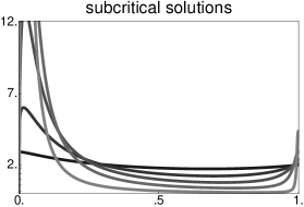
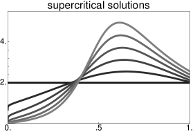
Figure 1: Solutions $G(y)$ to (17) with $D=1$ for $y\in[0,\,1]$ for different values of $G(1/2)<2$ (left) and $G(1/2)>2$ (center); moment $N(G)=\int_{0}^{1}G(y)d{y}$ in dependence on $G(1/2)$ (right).

We next discuss some numerical ODE simulations that illustrate how the solutions of (17) with $D=1$ depend on the value of $G(1/2)$. For $G(1/2)=2$ we get the trivial solution $G\equiv 2$. From now on, we refer to solutions with $G(1/2)>2$ as supercritical and to those with $G(1/2)<2$ as subcritical. These two types behave rather differently, see Figure 1, which shows the solutions for $G(1/2)\in\{0.2,\,0.6,\,1.0,\,1.4,\,1.8\}$ and $G(1/2)\in\{2.0,\,2.4,\,2.8,\,3.2,\,3.6,\,4.0\}$. Our numerical results indicate that each supercritical solution has precisely one local maximum between $1/2$ and $1$ but no local minimum. On the other hand, a subcritical solution has two local maxima close to $0$ and $1$, and a local minimum between $1/2$ and $1$, compare Figure 2, where ’variation near $1$’ refers to $G(y)-G(1)$.

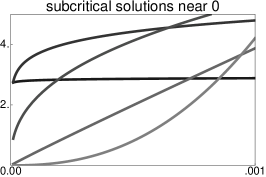
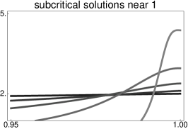
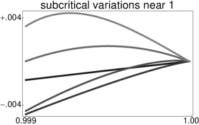
Figure 2: Subcritical solutions from Figure 1 for $y\approx 0$ and $y\approx 1$.

Figure 1 also shows how $\int_{0}^{1}G(y)dy$ depends on $G(1/2)$. Based on this, we conjecture that for every ${k_{0}}>2$ there exist two solutions to (16), one having a subcritical and the other having a supercritical shape. For ${k_{0}}=2$ there is a trivial self-similar solution. For ${k_{0}}<2$ there seem to be no self-similar solution. To support this conjecture, we now prove that there is no self-similar solution for ${k_{0}}\leq 1$: Integrating (16) we find $\lim_{z\rightarrow 1}G(z)=N$, so each solution to (16) satisfies $G(y)\sim y^{-2+{k_{0}}}$ as $y\rightarrow 0$, which contradicts $\int_{0}^{1}G(y)dy<\infty$. For $1<k_{0}<2$, however, this argument does not apply but our numerical results indicate there is still no singular solution.

4 Long-time behavior

To investigate the long time behaviour of solutions to (4) by numerical simulations we derive a discrete ”box model” which follows naturally from the physical interpretation. We assume the number of initial boxes $M_{\mathrm{b}}$ is sufficiently large (we choose $M_{\mathrm{b}}=200$ for all simulations) and consider the discrete times $t=\varepsilon{j}$ with $j\in\mathbb{N}$ and $\varepsilon=1/M_{\mathrm{b}}$. Moreover, we denote by $G(j,i)$ the number of particles with size $x\in(\varepsilon{i}-\varepsilon,\varepsilon{i})$ at time $t=1+\varepsilon{j}$, that means

$$G(j,i)={\varepsilon}^{-1}\int_{\varepsilon(i-1)}^{\varepsilon{i}}g(1+\varepsilon{j},x)dx$$

for all integers $j\geq 0$ and $i=1,\ldots,M_{\mathrm{b}}+j$. The disrete analogue to the evolution equation (4) is then given by

$$\frac{G(j+1,i)-G(j,i)}{\varepsilon}=\left\{\begin{aligned} &-\frac{k_{0}}{{N}(j)}G(j,i)G(j,M_{\mathrm{b}}+j+1-i)\quad&&0<i\leq j+M_{\mathrm{b}},\\ &0&&i>j+M_{\mathrm{b}}+1,\end{aligned}\right.$$

where $N(j)=\varepsilon\sum_{i=1}^{j+M_{\mathrm{b}}}G(j,i)$ and the value of $G(j,j+M_{\mathrm{b}}+1)$ is determined by the conservation of mass, i.e.,

$$G(j,j+M_{\mathrm{b}}+1)=\frac{\varepsilon}{2}\sum_{i=1}^{j+M_{\mathrm{b}}}\frac{k_{0}}{{N}(j)}G(j,i)G(j,M_{\mathrm{b}}+j+1-i).$$

We now present our numerical results for three different values of ${k_{0}}$ and three different sets of initial data. More precisely, we consider ${k_{0}}=1,2,3$ and assume that the initial data have Gaussian distributions with dispersion 0.3 and center at either $0.25$, $0.5$, or $0.75$.

For ${k_{0}}>2$ we expect convergence to one of the self-similar solutions. Numerical simulations suggest that the solution converges as $t\rightarrow\infty$ to the supercritical self-similar solution that corresponds to ${k_{0}}$. The same happens if the initial data is very close to the subcritical self-similar solution, and thus we can conclude that subcritical solutions are unstable. We failed to find a rigorous proof for this assertion, but the numerical evidence is strong. In Figure 3, we plot the scaled distributions after 0, 200, 1000 and 25000 steps (0, 1000, 25000 and 150000 if the center is at 0.25) for the three sets of initial data described above. The corresponding times are given by 0, 1, 5, and 125 (0, 5, 125, and 750). Along with these smooth curves we dotted the graph of the self-similar solution for ${k_{0}}=3$. As we see, the convergence is slowest when the center of the initial data is at 0.25.

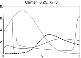
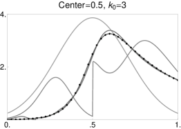
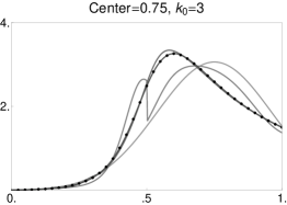
Figure 3: Convergence to self-similar form for ${k_{0}}=3$

For ${k_{0}}<2$ we observe a completely different behaviour. We do not see any convergence in the self-similar scaling. On the contrary, the solutions apparently converge pointwise in the original variables to a limit that depends on the initial data. We will prove the corresponding statement rigorously in Proposition 6 for ${k_{0}}<1/3$. Figure 4 shows the unscaled distributions for ${k_{0}}=1$, the initial data is the same as before. The five smooth curves represents numerical distributions after 0, 200, 1000, 5000 and 25000 steps.

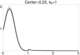
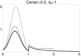
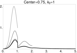
Figure 4: Convergence in the original variables for ${k_{0}}=1$

For ${k_{0}}=2$ we expect convergence to the trivial self-similar solution but the numerical simulations do not support this assertion. We can conclude that either the long time behaviour is more complicated or the convergence is extremely slow. Figure 5 contains the distributions after 0, 1000, 5000, 25000 and 150000 steps and the dotted plot of the self-similar solution. In the first picture we observe a behavior similar to that for ${k_{0}}<2$, that means the mass is cumulated near the origin. It will possibly eventually disappear but this was not the case after any number of steps that we were able to simulate. This happens also for ${k_{0}}>2$ if the initial data is more cummulated. For example, if we choose dispersion equal to 0.2 then 150000 steps is not enough to see the convergence for ${k_{0}}=3$ and center at $0.25$. This observation is not surprising because if the initial data is supported on $[0,1/2)$, then the evolution cannot start at all.

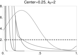
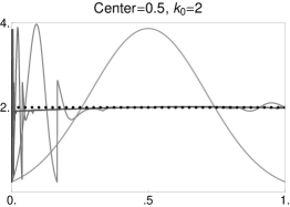
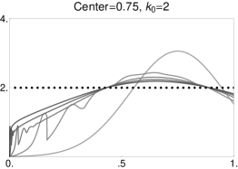
Figure 5: Evolution in self-similar variables for $d=2$

We conclude this section with a rigorous proof of a theorem supporting the conjecture that for ${k_{0}}<2$ there exists a limit function

$$\lim_{t\rightarrow\infty}g(t,x)=:g_{\infty}(x)>0.$$ (21)

Notice that (21) implies that the rescaled function $t^{2}g(t,yt):[0,1]\rightarrow\mathbb{R}$ converges, in the sense of probability measures, to a Dirac measure with positive mass.

Proposition 6.

1. If there exists $c_{0}>0$ such that $N(t)\geq c_{0}$ for all $t\geq 1$, then the relation (21) is satisfied.

2. If ${k_{0}}<1/3$ then $N(t)>N(1)/2$ for all $t\geq 1$.

Proof.

i) Suppose that $N(t)\geq c_{0}$. From (4) and (8) with $\tilde{g}=g$ we infer that

$$g(t,x)=g(max(1,x),x)\exp{\left(-{k_{0}}\int_{max(1,x)}^{t}\frac{g(s,s-x)}{N(s)}ds\right)}.$$

By assumption, we also have

$$\int_{max(1,x)}^{t}\frac{g(s,s-x)}{N(s)}ds\leq\frac{1}{c_{0}}\int_{max(1,x)}^{t}g(s,s-x)ds<\infty,$$

so $g(t,x)$ is bounded from below. Since it is also decreasing in $t$ for all $x$, there exists $g_{\infty}(x)$ as in (21).

ii) Due to (4), we have $-2N(t)N^{\prime}(t)={k_{0}}\int_{0}^{t}g(t,x)g(t,t-x)dx$ and by integration we obtain

$$N(1)^{2}-N(t)^{2} ={k_{0}}\int_{1}^{t}\int_{0}^{s}g(s,x)g(s,s-x)dxds$$ (22)

$$={k_{0}}\int_{0}^{t}\int_{max(1,x)}^{t}g(s,x)g(s,s-x)dsdx$$

$$\leq{k_{0}}\int_{0}^{t}g(max(1,x),x)\int_{max(1,x)}^{t}g(s,s-x)dsdx$$

$$\leq{k_{0}}\int_{0}^{t}g(max(1,x),x)\int_{0}^{t}g(max(1,s),s)dsdx$$

$$\leq{k_{0}}(2N(1)-N(t))^{2},$$

where the last inequality holds since

$$\int_{0}^{t}g(max(1,s),s)ds=\int_{0}^{1}g(1,s)ds+\int_{1}^{t}g(s,s)ds=N(1)+(N(1)-N(t)).$$

Now suppose that there exists $t>1$ such that $N(t)=N(1)/2$. By (22) we get ${k_{0}}\geq 1/3$ and using the continuity of $N$, we conclude that ${k_{0}}<1/3$ implies $N(t)>N(1)/2$ for all $t$. ∎

Acknowledgment

This work was supported by the EPSRC Science and Innovation award to the Oxford Centre for Nonlinear PDE (EP/E035027/1). Ondrej Budáč also gratefully acknowledges support through the SPP Foundation and by the Slovak Research and Development Agency under the contract No. APVV-0414-07.

References

- [1] A. Boudaoud, J. Bico and B. Roman, Elastocapillary coalescence: Aggregation and fragmentation with maximal size, Phys. Rev. E 76, 060102 (2007).
- [2] R. L. Drake, A general mathematical survey of the coagulation equation. In G.M. Hidy and J.R. Brock eds., Topics in current aerosol research (Part 2); International reviews in Aerosol Physics and Chemistry, Pergamon (1972), 201-376
- [3] M. Escobedo, S. Mischler and M. Rodriguez Ricard, On self-similarity and stationary problems for fragmentation and coagulation models, Ann. Inst. H. Poincaré Anal. Non Linéaire 22 (2005), 99-125.
- [4] N. Fournier and P. Laurençot, Existence of self-similar solutions to Smoluchowski’s coagulation equation, Comm. Math. Phys. 256, (2005) 589-609
- [5] N. Fournier and P. Laurençot, Well-posedness of Smoluchowski’s coagulation equation for a class of homogeneous kernels, J. Funct. Anal. 233, (2006) 351-379
- [6] S. K. Friedlander, Smoke, dust and haze: Fundamentals of aerosol dynamics. Wiley, New York, 1977.
- [7] T. Gallay and A. Mielke, Convergence results for a coarsening model using global linearization, J. Nonlinear Science 13 (2003), 311-346
- [8] F. Leyvraz, Scaling theory and exactly solvable models in the kinetics of irreversible aggregation, Phys. Reports 383 2/3 (2003), 95-212
- [9] G. Menon and R. L. Pego, Approach to self-similarity in Smoluchowski’s coagulation equations, Comm. Pure Appl. Math. 57 9 (2004), 1197-1232
- [10] G. Menon, B. Niethammer and R. L. Pego, Dynamics and self-similarity in min-driven clustering, Trans. AMS 362, 12 (2010), 6551-6590
- [11] M. Smoluchowski, Drei Vorträge über Diffusion, Brownsche Molekularbewegung und Koagulation von Kolloidteilchen, Phys. Zeitschr. 17 (1916), 557-599
- [12] R. M. Ziff, Kinetics of polymerization, 23, J. Statist. Phys. 23 (1980), 241-263