X-ray emitting MHD accretion shocks in classical T Tauri stars

Abstract

Context. Plasma accreting onto classical T Tauri stars (CTTS) is believed to impact the stellar surface at free-fall velocities, generating a shock. Current time-dependent models describing accretion shocks in CTTSs are one-dimensional, assuming that the plasma moves and transport energy only along magnetic field lines ($\beta\ll 1$).

Aims. We investigate the stability and dynamics of accretion shocks in CTTSs, considering the case of $\beta\;\lower 4.0pt\hbox{${\buildrel\displaystyle>\over{\sim}}$}\,1$ in the post-shock region. In these cases the 1D approximation is not valid and a multi-dimensional MHD approach is necessary.

Methods. We model an accretion stream propagating through the atmosphere of a CTTS and impacting onto its chromosphere, by performing 2D axisymmetric MHD simulations. The model takes into account the stellar magnetic field, the gravity, the radiative cooling, and the thermal conduction (including the effects of heat flux saturation).

Results. The dynamics and stability of the accretion shock strongly depends on the plasma $\beta$. In the case of shocks with $\beta>10$, violent outflows of shock-heated material (and possibly MHD waves) are generated at the base of the accretion column and strongly perturb the surrounding stellar atmosphere and the accretion column itself (modifying, therefore, the dynamics of the shock). In shocks with $\beta\approx 1$, the post-shock region is efficiently confined by the magnetic field. The shock oscillations induced by cooling instability are strongly influenced by $\beta$: for $\beta>10$, the oscillations may be rapidly dumped by the magnetic field, approaching a quasi-stationary state, or may be chaotic with no obvious periodicity due to perturbation of the stream induced by the post-shock plasma itself; for $\beta\approx 1$ the oscillations are quasi-periodic, although their amplitude is smaller and the frequency higher than those predicted by 1D models.

1 Introduction

In the last few years, high resolution ($R=600$) X-ray observations of several young stars accreting material from their circumstellar disk (TW Hya, BP Tau, V4046 Sgr, MP Mus and RU Lupi) suggested the presence of X-ray emission at temperature $T=2-5$ MK from plasma denser than $n_{\rm H}=10^{11}$ cm^-3 (Kastner et al. 2002; Schmitt et al. 2005; Günther et al. 2006; Argiroffi et al. 2007; Robrade & Schmitt 2007; Argiroffi et al. 2009). The emitting plasma is too dense to be enclosed inside coronal loop structures (Testa et al. 2004). Several authors suggested, therefore, that this soft X-ray emission component could be produced by the material accreting onto the star surface, flowing along the magnetic field lines of the nearly dipolar stellar magnetosphere, and heated to temperatures of few MK by a shock at the base of the accretion column (Calvet & Gullbring, 1998; Lamzin, 1998).

The idea that an accreting flow impacting onto a stellar surface leads to a shocked slab of material heated at millions degrees is not new. For instance, in the context of degenerate stars, several authors have studied the dynamics and energetic of accretion shocks and the effects of radiation on the formation, structure, and stability of the shocks (Langer et al., 1981, 1982; Chevalier & Imamura, 1982; Imamura, 1985; Chanmugam et al., 1985). Hujeirat & Papaloizou (1998) have also investigated the role of the magnetic field in confining the post-shock accreting material and in determining the evolution of the accretion shock. These studies have shown that the role of thermal and dynamical instabilities is critical to our ability to model radiative shock waves.

The first attempt to interpret the evidence of soft X-ray emission from dense plasma in Classical T Tauri stars (CTTSs) in terms of accretion shocks has quantitatively demonstrated that some non coronal features of the X-ray observations of TW Hya (Günther et al., 2007) and MP Mus (Argiroffi et al., 2007) could be explained through a simplified steady-flow shock model. However, steady models are known to be not a good approximation for radiative shocks, since they neglect the important effects of local thermal instabilities as well as global shock oscillations induced by radiative cooling (Sutherland & Dopita, 1993; Dopita & Sutherland, 1996; Safier, 1998; Sutherland et al., 2003a, b; Mignone, 2005).

In fact, the first time-dependent 1D models of radiative accretion shocks in CTTSs have shown quasi-periodic oscillations of the shock position induced by cooling (Koldoba et al., 2008; Sacco et al., 2008). In particular, Sacco et al. (2008) have developed a 1D hydrodynamic model including, among other important physical effects, a well tested detailed description of the stellar chromosphere and investigated the role of the chromosphere in determining the position and the thickness of the shocked region. For hydrodynamical simulations based on the parameters of MP Mus, Sacco et al. (2008) synthesized the high resolution X-ray spectrum, as it would be observed with the Reflection Grating Spectrometers (RGS) on board the XMM-Newton satellite, and found an excellent agreement with the observations.

Up to date time-dependent models of accretion shocks in CTTSs have been one dimensional, assuming that the plasma moves and transports energy only along magnetic field lines. This hypothesis is justified if the plasma $\beta\ll 1$ (where $\beta=$ gas pressure / magnetic pressure) in the shock-heated material. The photospheric magnetic field magnitude of CTTSs is believed to be around 1 kG (e.g. Johns-Krull et al. 1999). Such a strong stellar field is enough to confine efficiently accretion shocks with particle density below $10^{13}$ cm^-3 and temperature around 5 MK ($\beta<0.3$). However, recent polarimetric measurements indicate that, in some cases, the photospheric magnetic field strength could be less than 200 G (Valenti & Johns-Krull, 2004) and the plasma $\beta$ in the slab may be around 1 or even larger. In these cases, the magnetic field configuration in the post-shock region may change, influencing the physical structure of the material emitting in X-rays and the stability of the accretion shock.

The low-$\beta$ approximation was challenged by recent findings of Drake et al. (2009). In case of $\beta\ll 1$, the radiative shock instability is expected to lead to detectable periodic modulation of the X-ray emission from the shock-heated plasma, if the density and velocity of the accretion stream do not change over the time interval considered (in agreement with predictions of 1D models). However, the analysis of soft X-ray observations of the CTTS TW Hya (whose emission is believed to arise predominantly from accretion shocks) produced no evident periodic variations (Drake et al. 2009). These authors concluded, therefore, that 1D models may be too simple to describe the multi-dimensional structure of the shock and that the magnetic field may play an important role through the generation and damping of MHD waves.

In this paper, we investigate the stability and dynamics of accretion shocks in cases for which the low-$\beta$ approximation cannot be applied. We analyze the role of the stellar magnetic field in the dynamics and confinement of the slab of shock-heated material. To this end, we model an accretion stream propagating through the magnetized atmosphere of a CTTS and impacting onto its chromosphere, using 2D axisymmetric MHD simulations and, therefore, an explicit description of the ambient magnetic field. We investigate cases of $\beta\;\lower 4.0pt\hbox{${\buildrel\displaystyle>\over{\sim}}$}\,1$ in the post-shock region for which the deviations from 1D models are expected to be the largest. In Sect. 2 we describe the MHD model, and the numerical setup; in Sect. 3 we describe the results; in Sect. 4 we discuss the implications of our results and, finally, in Sect. 5, we draw our conclusions.

2 MHD modeling

The model describes an accretion stream impacting onto the surface of a CTTS. We assume that the accretion occurs along magnetic field lines linking the circumstellar disk to the star and consider only the portion of the stellar atmosphere close to the star.

The fluid is assumed to be fully ionized with a ratio of specific heats $\gamma=5/3$. The model takes into account the stellar magnetic field, the gravity, the radiative cooling, and the thermal conduction (including the effects of heat flux saturation). Since the magnetic Reynolds number $\gg 1$ considering the typical velocity ($10^{7}$ cm s^-1) and length scale ($10^{9}$ cm) of the system, the flow is treated as an ideal MHD plasma. The impact of the accretion stream is modeled by solving numerically the time-dependent MHD equations (written in non-dimensional conservative form):

$$\frac{\partial\rho}{\partial t}+\nabla\cdot(\rho\@vec{u})=0\leavevmode\nobreak\ ,$$ (1)

$$\frac{\partial\rho\@vec{u}}{\partial t}+\nabla\cdot(\rho\@vec{u}\@vec{u}-\@vec{B}\@vec{B})+\nabla P_{*}=\rho\@vec{g}\leavevmode\nobreak\ ,$$ (2)

$$\frac{\partial\rho E}{\partial t}+\nabla\cdot[\@vec{u}(\rho E+P_{*})-\@vec{B}(\@vec{u}\cdot\@vec{B})]=$$ (3)

$$\displaystyle\leavevmode\nobreak\ \leavevmode\nobreak\ \leavevmode\nobreak\ \leavevmode\nobreak\ \leavevmode\nobreak\ \leavevmode\nobreak\ \leavevmode\nobreak\ \leavevmode\nobreak\ \leavevmode\nobreak\ \leavevmode\nobreak\ \leavevmode\nobreak\ \leavevmode\nobreak\ \leavevmode\nobreak\ \leavevmode\nobreak\ \leavevmode\nobreak\ \leavevmode\nobreak\ \leavevmode\nobreak\ \leavevmode\nobreak\ \leavevmode\nobreak\ \leavevmode\nobreak\ \leavevmode\nobreak\ \leavevmode\nobreak\ \leavevmode\nobreak\ \leavevmode\nobreak\ \leavevmode\nobreak\ \rho\@vec{u}\cdot\@vec{g}-\nabla\cdot\@vec{F}_{\rm c}-n_{\rm e}n_{\rm H}\Lambda(T)\leavevmode\nobreak\ ,$$

$$\frac{\partial\@vec{B}}{\partial t}+\nabla\cdot(\@vec{u}\@vec{B}-\@vec{B}\@vec{u})=0\leavevmode\nobreak\ ,$$ (4)

where

$$P_{*}=P+\frac{B^{2}}{2}\leavevmode\nobreak\ ,\leavevmode\nobreak\ \leavevmode\nobreak\ \leavevmode\nobreak\ \leavevmode\nobreak\ \leavevmode\nobreak\ \leavevmode\nobreak\ \leavevmode\nobreak\ \leavevmode\nobreak\ \leavevmode\nobreak\ \leavevmode\nobreak\ \leavevmode\nobreak\ \leavevmode\nobreak\ \leavevmode\nobreak\ E=\epsilon+\frac{1}{2}u^{2}+\frac{1}{2}\frac{B^{2}}{\rho}\leavevmode\nobreak\ ,$$

are the total pressure, and the total gas energy (internal energy, $\epsilon$, kinetic energy, and magnetic energy) respectively, $t$ is the time, $\rho=\mu m_{H}n_{\rm H}$ is the mass density, $\mu=1.28$ is the mean atomic mass (assuming metal abundances 0.5 the solar values; Anders & Grevesse 1989), $m_{H}$ is the mass of the hydrogen atom, $n_{\rm H}$ is the hydrogen number density, $\@vec{u}$ is the gas velocity, $g$ is the gravity, $T$ is the temperature, $\@vec{B}$ is the magnetic field, $\@vec{F}_{\rm c}$ is the conductive flux, and $\Lambda(T)$ represents the optically thin radiative losses per unit emission measure (see Fig. 1) derived with the PINTofALE spectral code (Kashyap & Drake, 2000) with the APED V1.3 atomic line database (Smith et al., 2001), assuming the same metal abundances as before (as deduced from X-ray observations of CTTSs; Telleschi et al. 2007). We use the ideal gas law, $P=(\gamma-1)\rho\epsilon$.

Figure 1: Radiative losses for an optically thin plasma from the APED V1.3 atomic line database (Smith et al., 2001), assuming the metal abundances 0.5 the solar values (Anders & Grevesse 1989).

The thermal conductivity in an organized magnetic field is known to be highly anisotropic and it can be highly reduced in the direction transverse to the field. The thermal flux, therefore, is locally split into two components, along and across the magnetic field lines, $\@vec{F}_{\rm c}=F_{\parallel}\leavevmode\nobreak\ \@vec{i}+F_{\perp}\leavevmode\nobreak\ \@vec{j}$, where (see, for instance, Orlando et al. 2008)

$$\begin{array}[]{l}\displaystyle F_{\parallel}=\left(\frac{1}{[q_{\rm spi}]_{\parallel}}+\frac{1}{[q_{\rm sat}]_{\parallel}}\right)^{-1}\leavevmode\nobreak\ ,\\ \\ \displaystyle F_{\perp}=\left(\frac{1}{[q_{\rm spi}]_{\perp}}+\frac{1}{[q_{\rm sat}]_{\perp}}\right)^{-1}\leavevmode\nobreak\ ,\end{array}$$ (5)

to allow for a smooth transition between the classical and saturated conduction regime. In Eqs. 5, $[q_{\rm spi}]_{\parallel}$ and $[q_{\rm spi}]_{\perp}$ represent the classical conductive flux along and across the magnetic field lines (Spitzer, 1962)

$$\begin{array}[]{l}\displaystyle[q_{\rm spi}]_{\parallel}=-\kappa_{\parallel}[\nabla T]_{\parallel}\approx-9.2\times 10^{-7}T^{5/2}\leavevmode\nobreak\ [\nabla T]_{\parallel}\\ \\ \displaystyle[q_{\rm spi}]_{\perp}=-\kappa_{\perp}[\nabla T]_{\perp}\approx-3.3\times 10^{-16}\frac{n^{2}_{\rm H}}{T^{1/2}B^{2}}\leavevmode\nobreak\ [\nabla T]_{\perp}\end{array}$$ (6)

where $[\nabla T]_{\parallel}$ and $[\nabla T]_{\perp}$ are the thermal gradients along and across the magnetic field, and $\kappa_{\parallel}$ and $\kappa_{\perp}$ (in units of erg s^-1 K^-1 cm^-1) are the thermal conduction coefficients along and across the magnetic field lines, respectively. The saturated flux along and across the magnetic field lines, $[q_{\rm sat}]_{\parallel}$ and $[q_{\rm sat}]_{\perp}$, are (Cowie & McKee, 1977)

$$\begin{array}[]{l}\displaystyle[q_{\rm sat}]_{\parallel}=-\mbox{sign}\left([\nabla T]_{\parallel}\right)\leavevmode\nobreak\ 5\phi\rho c_{\rm s}^{3},\\ \\ \displaystyle[q_{\rm sat}]_{\perp}=-\mbox{sign}\left([\nabla T]_{\perp}\right)\leavevmode\nobreak\ 5\phi\rho c_{\rm s}^{3},\end{array}$$ (7)

where $c_{\rm s}$ is the isothermal sound speed, and $\phi$ is a number of the order of unity; we set $\phi=1$ according to the values suggested for stellar coronae (Giuliani, 1984; Borkowski et al., 1989; Fadeyev et al., 2002, and references therein).

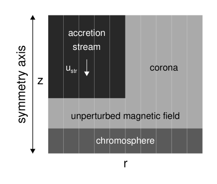
Figure 2: Initial geometry of the system in cylindrical coordinates. The stellar surface lies on the $r$ axis and the unperturbed stellar magnetic field is uniform and oriented along the $z$ axis (vertical lines). The accretion stream propagates downwards through the stellar corona with velocity $u_{\mathrm{str}}$. The $z$-axis is the symmetry axis of the problem.

We solve the MHD equations using cylindrical coordinates in the plane $(r,z)$, assuming axisymmetry and the stellar surface lying on the $r$ axis (see Fig. 2). The initial unperturbed stellar atmosphere is assumed to be magneto-static and to consist of a hot (maximum temperature $\approx 10^{6}$ K) and tenuous ($n_{\rm H}\approx 2\times 10^{8}$ cm^-3) corona linked through a steep transition region to an isothermal chromosphere that is uniformly at temperature $10^{4}$ K and is $8.5\times 10^{8}$ cm thick (see Fig. 3). The choice of an isothermal chromosphere is adopted for ease of modeling, and different choices of more detailed chromospheric models have been shown not to lead to significantly different results (Sacco et al. 2009, in preparation). The unperturbed stellar magnetic field is uniform, oriented along the $z$ axis and perpendicular to the stellar surface. The gravity is calculated assuming the star mass $M=1.2M_{\sun}$ and the star radius $R=1.3R_{\sun}$ which is appropriate for the CTTS MP Mus (see Argiroffi et al. 2007). Different choices of stellar parameters should not lead to different results.

Figure 3: Initial hydrogen number density (dashed line) and temperature (dotted line) as a function of height above the stellar surface, $z$, for the unperturbed stellar atmosphere.

The accretion stream is assumed to be constant and propagates along the $z$ axis. Initially the stream is in pressure equilibrium with the stellar corona and has a circular cross-section with radius $r_{\mathrm{str}}=5\times 10^{9}$ cm; its radial density distribution is given by

$$n_{\mathrm{str}}(r)=n_{\rm cor}+\frac{n_{\rm str0}-n_{\rm cor}}{\cosh\left[\sigma\left(r/r_{\rm str}\right)^{\sigma}\right]}\leavevmode\nobreak\ \leavevmode\nobreak\ \leavevmode\nobreak\ ,$$ (8)

where $n_{\mathrm{str0}}$ and $n_{\rm cor}$ are the hydrogen number density at the stream center and in the corona, and $\sigma=20$ is a steepness parameter. The above distribution describes a thin shear layer ($\sim 0.1\leavevmode\nobreak\ r_{\rm str}$) around the stream that smooths the stream density to the value of the surrounding medium and maintains numerical stability, allowing for a smooth transition of the Alfvén speed at the interface between the stream and the stellar atmosphere. The stream temperature is determined by the pressure balance across the stream boundary.

The velocity of the stream along the $z$ axis also has a radial profile:

$$u_{\mathrm{str}}(r)=\frac{u_{\rm str0}}{\cosh\left[\sigma\left(r/r_{\rm str}\right)^{\sigma}\right]}\leavevmode\nobreak\ \leavevmode\nobreak\ \leavevmode\nobreak\ ,$$ (9)

where $u_{\mathrm{str0}}$ is the free fall velocity at the center of the stream. The smooth shear layer of velocity avoids the growth of random perturbations with wavelengths of the order of the grid size (e.g. Bodo et al. 1994).

The simulations presented here describe the evolution of the system for a time interval of about 3000 s. We used the accretion parameters (velocity and density) that match the soft X-ray emission of MP Mus (Argiroffi et al. 2007), namely $n_{\rm str0}=10^{11}$ cm^-3 and $u_{\rm str0}=-500$ km s^-1 at a height $z=2.4\times 10^{10}$ cm above the stellar surface. The initial field strengths of $|\@vec{B}_{\mathrm{0}}|=1,\,10,\,50$ G in the unperturbed stellar atmosphere (see Table 1) maintain $\beta\;\lower 4.0pt\hbox{${\buildrel\displaystyle>\over{\sim}}$}\,1$ in the post-shock region, where $\beta=P/(B^{2}/8\pi)$ is the ratio of thermal to magnetic pressure. For instance, $|\@vec{B}_{\mathrm{0}}|=10$ G corresponds to $\beta$ ranging between $\approx 10^{4}$, at the base of the chromosphere, and $\approx 10^{-2}$ up in corona. We also performed a 1D hydrodynamic simulation in order to provide a baseline for the 2D calculations. This simulation corresponds to the strong magnetic field limit ($\beta\ll 1$), in which the plasma moves and transports energy exclusively along the magnetic field lines (see Sacco et al. 2008).

Table 1: Relevant parameters of the simulations

Name of	$|\@vec{B}_{\mathrm{0}}|$ [G]	Geometry	Mesh	time
simulation				covered [s]
HD-1D	-	Cartes. 1D	1024	3000
By-01	1	cylind. 2D	$512\times 1024$	3000
By-10	10	cylind. 2D	$512\times 1024$	4000
By-50	50	cylind. 2D	$512\times 1024$	3000
By-01-HR	1	cylind. 2D	$1024\times 2048$	1000
By-10-HR	10	cylind. 2D	$1024\times 2048$	1000
By-50-HR	50	cylind. 2D	$1024\times 2048$	2000

The calculations described in this paper were performed using pluto (Mignone et al., 2007), a modular, Godunov-type code for astrophysical plasmas. The code provides a multiphysics, multialgorithm modular environment particularly oriented toward the treatment of astrophysical flows in the presence of discontinuities such as in the case treated here. The code was designed to make efficient use of massively parallel computers using the message-passing interface (MPI) library for interprocessor communications. The MHD equations are solved using the MHD module available in pluto which is based on the Harten-Lax-van Leer Discontinuities (HLLD) approximate Riemann solver (Miyoshi & Kusano 2005). Miyoshi & Kusano (2005) have shown that the HLLD algorithm can exactly solve isolated discontinuities formed in the MHD system and, therefore, the adopted scheme is particularly appropriate to describe accretion shocks. The evolution of the magnetic field is carried out using the constrained transport method of Balsara & Spicer (1999) that maintains the solenoidal condition at machine accuracy. pluto includes optically thin radiative losses in a fractional step formalism (Mignone et al., 2007), which preserve $2^{nd}$ time accuracy, being the advection and source steps at least $2^{nd}$ order accurate; the radiative losses $\Lambda$ values are computed at the temperature of interest using a table lookup/interpolation method. The thermal conduction is solved with an explicit scheme that adds the parabolic contributions to the upwind fluxes computed at cell interfaces (Mignone et al., 2007). Such a scheme is subject to a rather restrictive stability condition (i.e. $\Delta t<(\Delta x)^{2}/(2\eta)$, where $\eta$ is the maximum diffusion coefficient), being the thermal conduction timescale generally shorter than the dynamical one (e.g. Hujeirat & Camenzind 2000; Hujeirat 2005; Orlando et al. 2005, 2008).

The symmetry of the problem allows us to solve the MHD equations in half of the spatial domain with the stream axis coincident with the $z$ axis. The 2D cylindrical $(r,z)$ mesh extends between 0 and $1.2\times 10^{10}$ cm in the $r$ direction and between 0 and $2.4\times 10^{10}$ cm in the $z$ direction and consists of a uniform grid with $512\times 1024$ grid points. Additional runs were done with setups identical to those used for runs By-01, By-10, and By-50 but with higher resolution ($1024\times 2048$ grid points; see Tab. 1) to evaluate the effect of spatial resolution (see Sect. 3.4); the simulations with higher resolution cover a time interval of about 1000 s.

We use fixed boundary conditions at the lower ($z=0$) boundary, imposing zero material and heat flux across the boundary. With this condition, matter may progressively accumulate at the base of the chromosphere; we have estimated that this effect may become significant on timescales a factor 100 longer than than those explored by our simulations. Axisymmetric boundary conditions are imposed at $r=0$ (i.e. along the symmetry axis of the problem), a constant inflow at the upper boundary ($z=2.4\times 10^{10}$ cm) for $r\leq r_{\rm str}$, and free outflow elsewhere.

3 Results

3.1 One-dimensional reference model

The results of our 1D reference hydrodynamic simulation, HD-1D, are analogous to those discussed by Sacco et al. (2008): the impact of the accretion stream onto the stellar chromosphere generates a reverse shock which propagates through the accretion column, producing a hot slab. According to Sacco et al., the expected temperature, $T_{\mathrm{slab}}$, and maximum thickness, $D_{\mathrm{slab}}$, of the slab, in the strong shock limit (Zel’Dovich & Raizer 1967) are:

$$T_{\mathrm{slab}}\approx\frac{3}{32}\frac{\mu m_{\mathrm{H}}}{k_{\mathrm{B}}}u_{\mathrm{str0}}^{2}\approx 5\leavevmode\nobreak\ \mbox{MK}\leavevmode\nobreak\ ,$$ (10)

$$D_{\mathrm{slab}}\approx 4.2\times 10^{2}\frac{u_{\mathrm{str0}}}{n_{\mathrm{str0}}}T_{\mathrm{slab}}^{3/2}\approx 2.5\times 10^{9}\leavevmode\nobreak\ \mbox{cm}\leavevmode\nobreak\ ,$$ (11)

where $k_{\mathrm{B}}$ is the Boltzmann constant.

Fig. 4 shows the time-space plot of the temperature evolution for run HD-1D. The base of the hot slab penetrates the chromosphere (the dashed line in Fig. 4 marks the initial position of the transition region between the chromosphere and the corona) down to the position at which the ram pressure, $P_{\mathrm{ram}}=\rho_{\mathrm{str0}}u_{\mathrm{str0}}^{2}$, of the post-shock plasma equals the thermal pressure of the chromosphere (Sacco et al. 2008). As evident from the figure, the shock front is not steady and the amplitude and period of the pulses rapidly reach stationary values as the initial transient disappears. The shock position oscillates with a period of $\approx 600$ s due to strong radiative cooling at the base of the slab, which robs the post-shock plasma of pressure support, causing the material above the cooled layer to collapse back before the slab expands again (see Sacco et al. 2008 for a detailed description of the system evolution). The maximum thickness of the slab is $D_{\mathrm{slab}}\approx 2.5\times 10^{9}$ cm, in agreement with the prediction (see Eq. 11). The post-shock plasma reaches the temperature $T_{\mathrm{slab}}\approx 5-7$ MK during the expansion phase, and $T_{\mathrm{slab}}\approx 2-4$ MK during the cooling phase.

As already mentioned, the evolution of the accretion shock described by the 1D reference model is appropriate if the magnetic field lines can be considered rigid to any force exerted by the accreting plasma flowing along the lines ($\beta\ll 1$). In case of plasma $\beta$ values around 1 or even higher, the hot slab is expected to be only partially confined by the magnetic field and flow can occur sideways because of the strong pressure of the post-shock plasma and may ultimately perturb the dynamics of the shock itself. Moreover, 2D or 3D structures leading to strongly cooling zones are expected to develop in the post-shock plasma if the latter is characterized by $\beta\;\lower 4.0pt\hbox{${\buildrel\displaystyle>\over{\sim}}$}\,1$. In this case, Sutherland et al. (2003a) showed that the evolution of 1D and 2D radiative shocks may be significantly different.

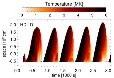
Figure 4: Time-space plot of the temperature evolution for run HD-1D. The spatial extent of the shock lies in the vertical direction at any instant in time. The dashed line marks the initial position of the transition region between the chromosphere and the corona.

3.2 Two-dimensional radiative MHD shock model

The cases of $\beta\;\lower 4.0pt\hbox{${\buildrel\displaystyle>\over{\sim}}$}\,1$ are described by our 2D model. The main differences on the evolution from the 1D model are expected to occur at the border of the stream where the shock-heated plasma might be not confined efficiently by the magnetic field; so we focus our attention there.

Fig. 5 shows the spatial distribution of temperature (on the left) and plasma $\beta$ (on the right) for runs By-01, By-10, and By-50 at time $t=530$ s (at early stage of evolution). Movies showing the complete evolution of 2D spatial distributions of mass density (on the left) and temperature (on the right), in log scale, for runs By-01, By-10, and By-50 are provided as on-line material. The accretion flow follows the magnetic field lines and impacts onto the chromosphere, forming a hot slab at the base of the stream with temperatures $\approx 5$ MK and $\beta\;\lower 4.0pt\hbox{${\buildrel\displaystyle>\over{\sim}}$}\,1$. In all the cases, the slab is rooted down in the chromosphere, where the thermal pressure equals the ram pressure, and part ($\approx 1/3$) of the shock column is buried under a column of optically thick material and may suffer significant absorption. In runs By-01 and By-10, the dense hot plasma behind the shock front causes a pressure driven flow parallel to the stellar surface, expelling accreted material sideways (see upper and middle panels in Fig. 5; see also on-line movies for runs By-01 and By-10). This outflow strongly perturbs the shock dynamics and is absent in the 1D shock model. As expected, this feature determines the main differences between these 2D and the 1D simulations.

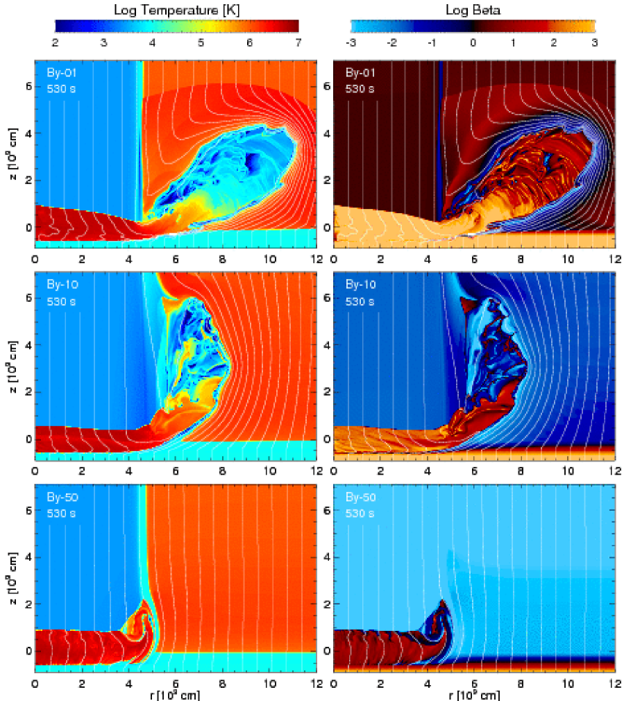
Figure 5: Temperature (left panels) and plasma $\beta$ (right panels) distributions in the $(r,z)$ plane, in log scale, in the simulations By-01, By-10, and By-50 at time $t=530$ s. The initial position of the transition region between the chromosphere and the corona is at $z=0$. The magnetic field is initially oriented along the $z$ axis; the white lines mark magnetic field lines.

In run By-01, the magnetic field is too weak to confine the post-shock plasma ($\beta\approx 10^{4}$ at the border of the slab) and a conspicuous amount of material continuously escapes from the border of the accretion column at its base where the flow impacts onto the stellar surface. The maximum escape velocity is comparable to the free-fall velocity, $u_{\mathrm{str0}}$, and this outflow acts as an additional cooling mechanism. The resulting outflow advects and stretches the magnetic field lines (see upper panels in Fig. 5), taking the material away from the accretion column and strongly perturbing the stellar atmosphere even at several stream radii. As a result of the outflow, a strong component of $\@vec{B}$ perpendicular to the stream velocity ($B_{\mathrm{r}}\approx 0.3|\@vec{B}_{\mathrm{0}}|$) appears in the post-shock region (see upper panels in Fig. 5). As discussed by Toth & Draine (1993), the presence of even a small magnetic field perpendicular to the flow can stabilize the overstable oscillations. In fact, at variance with the force due to gas pressure, the Lorentz force is not affected by cooling processes (see also Hujeirat & Papaloizou 1998) and this mechanism may contribute to stabilize the shock oscillations (see the on-line movie).

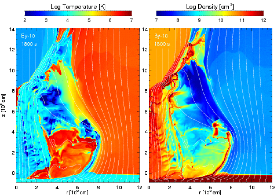
Figure 6: Temperature (left panel) and mass density (right panel) distributions in the $(r,z)$ plane, in log scale, in the simulation By-10, at time $t=1800$ s. The white lines mark magnetic field lines.

In the intermediate run By-10, the magnetic field is trapped at the head of the escaped material, leading to a continuous increase of the magnetic pressure and field tension there. As a result, the escaped material is kept close to the accretion column by the magnetic field (at variance with the By-01 case) and, eventually, may perturb the stream itself. In fact, the escaped material accumulates around the accretion column, forming a growing sheath of turbulent material gradually enveloping the stream. The magnetic pressure and field tension increase at the interface between the ejected material and the surrounding medium, pushing on the material and forcing it to plunge into the stream after $\approx 1.3$ ks. Fig. 6 shows the temperature and mass density distributions at time $t=1.8$ ks, when the expelled material has already entered into the stream and has strongly perturbed the accretion column (see also the on-line movie to follow the complete evolution). As a result of the stream perturbation, the hot slab may temporarily disappear altogether as shown in Fig. 6. In this phase, the region of impact of the stream onto the chromosphere is characterized by a rather complex structure with knots and filaments of material and may involve possible mixing of plasma of the surrounding corona with accretion material.

In the By-50 case, the post-shock plasma is confined efficiently by the magnetic field and no outflow of accreted material forms (see lower panels in Fig. 5). In particular, $\beta\approx 10^{-4}$ and the magnetic pressure $P_{\mathrm{B}}\approx 100P_{\mathrm{ram}}$ at the stream border, where $P_{\mathrm{ram}}=\rho u^{2}$ is the ram pressure. The 2D shock, therefore, evolves similarly to the 1D overstable shock simulation, alternating phases of expansion and collapse of the post-shock region (see the on-line movie). The maximum thickness of the slab is $D_{\mathrm{slab}}\approx 1.4\times 10^{9}$ cm, i.e. less than in the 1D case by a factor $\approx 1.8$. This result is analogous to that described by Sutherland et al. (2003a) in the case of 2D hydrodynamic radiative shocks and is explained as due to the formation of denser knots of more rapidly cooling gas. Note that, at variance with our MHD simulations, the hydrodynamic model of Sutherland et al. (2003a) does not include the thermal conduction. In our simulations, the thermal conduction acts as an additional cooling mechanism of the hot slab, draining energy from the shock-heated plasma to the chromosphere, and partially contrasts the radiative cooling. Depending on the temperature of the shock and on the plasma $\beta$, therefore, the thermal conduction may lead to significant differences between our results and those of Sutherland et al. (2003a).

Fig. 7 shows snapshots of the evolution of temperature distribution (in linear scale) in run By-50. The post-shock region gets larger ($t=1.05$ ks), reaches the maximum extension ($t=1.15$ ks), and collapses ($t=1.25$ ks); the cycle then repeats and the slab begins to get larger again ($t=1.35$ ks). Although the magnetic field is strong enough to confine the post-shock plasma, the plasma $\beta$ is slightly larger than 1 inside the slab and the 1D approximation is not valid there. As in the 2D hydrodynamic simulations (Sutherland et al. 2003a), therefore, complex 2D cooling structures, including knots and filaments of dense material, form there due to the thermal instability of the post-shock plasma (see $t=1.15$ ks in Fig. 7). As discussed by Sutherland et al. (2003a), these 2D complex structures lead to zones cooling more efficiently than those in 1D models (by virtue of the increased cold-hot gas boundary) and, therefore, the amplitude of oscillations is expected to be reduced. It is worth noting that the similarity of our results with those of the hydrodynamic models is due to the fact that, in run By-50, $\beta\;\lower 4.0pt\hbox{${\buildrel\displaystyle>\over{\sim}}$}\,1$ in the slab and 2D cooling structures can form. In the case of $\beta\ll 1$ everywhere in the slab, we expect that the stream can be considered as a bundle of independent fibrils (each of them describable in terms of 1D models), and the 2D MHD simulations would produce the same results of 1D models.

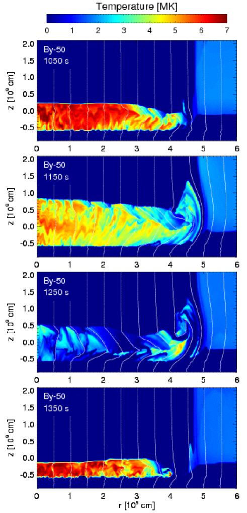
Figure 7: Temperature distribution in the $(r,z)$ plane, in linear scale, in the simulation By-50, at the labeled times. The white lines mark magnetic field lines.

We also study the global time evolution of 2D shocks by deriving time-space plots of the temperature evolution analogous to that derived for the 1D reference simulation (in order to compare directly our 1D and 2D results). From the 2D spatial distributions of temperature and mass density, we first derive profiles of temperature along the $z$-axis, by averaging the emission-measure-weighted temperature along the $r$-axis for $r<4\times 10^{9}$ cm (i.e. 80% of the stream radius); then, from these profiles, we derive the time-space plots of the average temperature evolution.

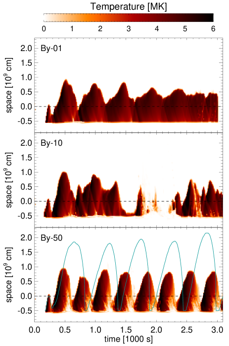
Figure 8: As in Fig. 4 for the 2D simulations By-01 (top), By-10 (middle) and By-50 (bottom). The blue curve in the bottom panel marks the shock position derived in the 1D reference model, HD-1D.

Fig. 8 shows the results for runs By-01, By-10, and By-50, and can be compared with Fig. 4. In all the cases, the amplitude of the shock oscillations is smaller than that observed in the 1D reference model. In runs By-01 and By-10, the evolution of the 2D shock is markedly different from that of the 1D shock (compare Fig. 4 with top and middle panels in Fig. 8): in run By-01, the oscillations of the shock are stabilized after 2.5 ks and the solution approaches a quasi-stationary state; in run By-10, the oscillations appear chaotic without an evident periodicity (at least in the time lapse explored here). As discussed before, the stabilization of the shock oscillations in the former case is due to a small magnetic field component perpendicular to the flow (Toth & Draine 1993), whereas the chaotic oscillations in the latter case are due to the continuous stream perturbation by the material ejected sideways at the stream base (see Fig 6). In the run By-50, the shock evolves somewhat similarly to the 1D overstable shock simulation, showing several expansion and collapse complete cycles of the post-shock region (see lower panel in Fig. 8). However, as already discussed before, some important differences arises: by comparing By-50 with HD-1D, the oscillations are reduced in amplitude by a factor $\sim 1.8$ and occur at higher frequency (period $P_{\mathrm{sh}}\approx 300$ s).

3.3 Effect of stream parameters

The details of the shock evolution described in this paper depend on the model parameters adopted. In particular, the temperature of the shock-heated plasma is determined by the free-fall velocity with which the plasma impacts onto the star (Eq.10); the stand-off height of the hot slab generated by the impact depends on the velocity and density of the stream (see Eq. 11). Assuming a typical value for the free-fall velocity of $400-500$ km s^-1 (leading to temperatures of $\approx 3-5$ MK, as deduced from observations), the maximum thickness of the slab is determined only by the density of the stream: the heavier the stream, the thinner is expected the slab. Also the sinking of the stream down in the chromosphere depend on the stream density and velocity at impact. In fact, we find that the slab penetrates the chromosphere down to the position at which the ram pressure, $\rho_{\mathrm{str0}}u_{\mathrm{str0}}^{2}$, of the post-shock plasma equals the thermal pressure of the chromosphere (see also Sacco et al. 2008). As a result, heavier streams are expected to sink more deeply into the chromosphere.

In the case of $\beta>1$, the shock evolution is expected to be influenced also by the stream radius, $r_{\mathrm{str}}$. In fact, as shown by our simulations, the complex plasma dynamics close to the border of the stream (e.g. the generation of outflows of accreted plasma; see runs By-01 and By-10) may affect the shock evolution in the inner portion of the slab. The shock evolution is expected to be modified in the whole slab if the oscillation period of the shock, $P_{\mathrm{sh}}$, is larger than the dynamical response time of the post-shock region, which can be approximated as the sound crossing time of half slab: $\tau_{\rm dyn}\sim r_{\mathrm{str}}/c_{\mathrm{s}}$, where $c_{\mathrm{s}}$ is the isothermal sound speed. In the cases discussed in this paper, the oscillation period is $P_{\mathrm{sh}}\approx 300$ s, and the sound crossing time of the slab is $\tau_{\rm dyn}\approx 200$ s; as shown by our simulations, the shock evolution is modified in the whole slab. Assuming an accretion stream with twice the radius considered here, we find $\tau_{\rm dyn}\approx 400$ s, and the region at the center of the slab should not be affected by the plasma dynamics at the stream border. In this case, we expect quasi-periodic shock oscillations (analogous to those described by run By-50) at the center of the stream and a strongly perturbed shock at the stream border.

3.4 Effect of spatial resolution

In problems involving radiative cooling, the spatial resolution and the numerical diffusion play an important role in determining the accuracy with which the dynamics of the system is described. In particular, in the case of radiative shocks, we expect that the details of the plasma radiative cooling depend on the numerical resolution: a higher resolution may lead to different peak density and hence influence the cooling efficiency of the gas, and therefore the amplitude and frequency of shock oscillations. In the simulations presented here, the thermal conduction partially contrasts the radiative cooling alleviating the problem of numerical resolution (see, for instance, Orlando et al. 2008).

In order to check if our adopted resolution is sufficient to capture the basic shock evolution over the time interval considered, we repeated simulations By-01, By-10, and By-50 but with twice the spatial resolution (runs By-01-HR, By-10-HR, and By-50-HR). The efficiency of radiative cooling is expected to be the largest in the model with $|\@vec{B}_{\mathrm{0}}|=50$ G, because there is no loss of material through sideways outflows. In fact, quasi-periodic oscillations of the accretion shock occur (see Fig. 8) and make this case adequate for a comparison of different spatial resolutions. Since this case is one of the most demanding for resolution, it can be considered a worst case comparison of convergence.

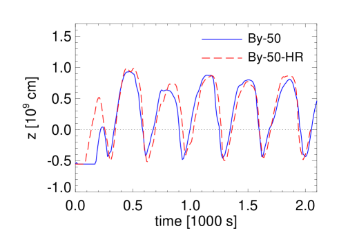
Figure 9: Evolution of the averaged shock-front location for runs By-50 (solid blue line) and By-50-HR (dashed red line). The dotted line marks the initial position of the transition region between the chromosphere and the corona.

Fig. 9 compares the evolution of the averaged shock-front location for runs By-50 and By-50-HR. The main differences between the simulations appear in the first bounce which starts earlier and is larger by a factor $\approx 2$ in By-50-HR than in By-50. The first expansion of the hot slab occurs after that the stream has penetrated the chromosphere down to the position where the ram pressure of the shock-heated material equals the thermal pressure of the chromosphere. The first bounce is a transient, therefore, and in fact its amplitude and width are different from those of subsequent bounces in all the simulations examined. On the other hand, Fig. 9 clearly shows that, apart from the first bounce, in general, the results of the two simulations agree quite well, showing differences $<10\%$. We expect, therefore, that increasing the spatial resolution, the results of our simulations may slightly change quantitatively (e.g. the amplitude of oscillations) but not qualitatively.

4 Discussion

4.1 Distribution of emission measure vs. temperature of the shock-heated plasma

As discussed in the introduction, there is a growing consensus that two distinct plasma components contribute to the X-ray emission of CTTSs: the stellar corona and the accretion shocks. This idea has been challenged recently by Argiroffi et al. (2009), who compared the distributions of emission measure, EM$(T)$, of two CTTSs with evidence of X-ray emitting dense plasma (MP Mus and TW Hya) with that of a star (TWA 5) with no evidence of accretion (i.e. only the coronal component is present) and with the EM($T$) derived from a 1D hydrodynamic model of accretion shocks (i.e. only the shock-heated plasma component is present; Sacco et al. 2008). They proved that the EM($T$) of MP Mus and TW Hya can be naturally interpreted as due to a coronal component, dominating at temperatures $T>5$ MK, plus a shock-heated plasma component, dominating at $T<5$ MK.

In case of shocks with $\beta>1$, our simulations show that the distributions of temperature and density at the base of the accretion column can be rather complex (see, for instance, Fig. 7). It is interesting, therefore, to investigate how the EM$(T)$ of the shock-heated plasma changes with $\beta$ and if it is possible to derive a diagnostics of the plasma-$\beta$ in the post-shock region.

In order to derive the EM($T$) distribution of the accretion region from the models, we first recover the 3D spatial distributions of density and temperature by rotating the corresponding 2D distributions around the symmetry $z$ axis ($r=0$). The emission measure in the $j$th domain cell is calculated as ${\rm em}_{\rm j}=n_{\rm Hj}^{2}V_{\rm j}$, where $n_{\rm Hj}^{2}$ is the particle number density in the cell, and $V_{\rm j}$ is the cell volume. The EM($T$) distribution is then derived by binning the emission measure values into slots of temperature; the range of temperature [$5<\log T(\mbox{K})<8$] is divided into 15 bins, all equal on a logarithmic scale ($\Delta\log T=0.2$).

Fig. 10 shows the EM($T$) distributions averaged over 3 ks for runs By-01, By-10, and By-50, together with the average EM$(T)$ derived from our 1D reference model HD-1D (blue dashed lines). The figure shows the EM($T$) distributions of plasma with density $n_{\mathrm{H}}>10^{11}$ cm^-3 (black) and $10^{10}<n_{\mathrm{H}}<10^{11}$ cm^-3 (red). The 2D MHD models have been normalized in order to have an X-ray luminosity $L_{\mathrm{X}}\approx 4\times 10^{29}$ erg in the band $[0.5-8.0]$ keV, in agreement with the luminosity derived from the low-temperature ($\log T<6.7$) portion of the EM($T$) distribution of MP Mus (Argiroffi et al. 2009). This is obtained assuming that $\approx 10$ accretion streams similar to that modeled here are present simultaneously. The 1D model has been normalized in order to match the EM peak in By-50. Inspecting Fig. 10 we note that: i) in all the cases, the EM($T$) has a peak at $\sim 5$ MK and a shape compatible with those observed in MP Mus and TW Hya and attributed to shock-heated material (e.g. Argiroffi et al. 2009); ii) most of the X-ray emission arises from shock-heated plasma with density $>10^{11}$ cm^-3 regardless of the $\beta$ (i.e. the most dense component of the post-shock region dominates); iii) the slope of the ascending branch of the EM($T$) distribution is comparable in runs By-50 and HD-1D, and gets steeper for decreasing values of $\beta$. The time-averaged X-ray luminosity derived from these EM($T$) distributions ranges between $5\times 10^{29}$ erg (run By-10) and $8\times 10^{29}$ erg (run By-01), having the X-ray luminosity only a weak dependence on the plasma $\beta$.

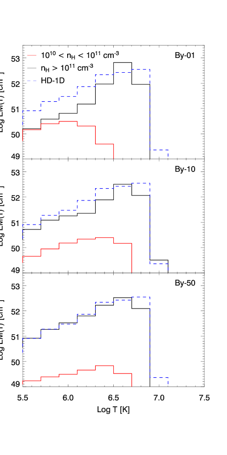
Figure 10: Distributions of emission measure vs. temperature, averaged over 3 ks, for runs By-01, By-10, and By-50. Black (red) lines mark the average EM($T$) distributions of plasma with density $n_{\mathrm{H}}>10^{11}$ cm^-3 ($10^{10}<n_{\mathrm{H}}<10^{11}$ cm^-3); dashed blue lines mark the average EM($T$) distribution for the 1D reference model HD-1D.

Our model supports, therefore, the idea that dense shock-heated plasma may contribute significantly to the low temperature portion of the EM($T$) distributions of CTTSs regardless of the $\beta$ value. We also suggest that the shape of the EM($T$) might be used as a diagnostics of $\beta$ in the post-shock region, if the coronal contribution to the low temperature tail can be neglected.

4.2 Mass accretion rates

Time-dependent models of radiative accretion shocks provide a strong theoretical support to the hypothesis that soft X-ray emission from CTTSs arises from shocks due to the impact of the accretion columns onto the stellar surface. However, several points remain still unclear. Among these, the most puzzling is probably the fact that the mass accretion rates derived from X-rays, Ṁ_X, are consistently lower by one or more orders of magnitude than the corresponding Ṁ values derived from UV/optical/NIR observations (e.g. Drake 2005; Schmitt et al. 2005; Günther et al. 2007; Argiroffi et al. 2009, Curran et al. 2009, in preparation). We have here the opportunity to discuss the problem of the accretion rate, in particular focusing on the cases with $\beta\;\lower 4.0pt\hbox{${\buildrel\displaystyle>\over{\sim}}$}\,1$ in the post-shock region.

The model parameters adopted in this paper describe a stream with an accretion rate of $\approx 9\times 10^{-12}M_{\mathrm{\odot}}$ yr^-1. According with the discussion in Sect. 4.1, $\approx 10$ streams are needed to match the soft X-ray luminosity of MP Mus. In this case the accretion rate is $\approx 9\times 10^{-11}M_{\mathrm{\odot}}$ yr^-1, which is in nice agreement with that deduced from observations, namely Ṁ${}_{\mathrm{X}}=5-8\times 10^{-11}M_{\mathrm{\odot}}$ yr^-1 (Argiroffi et al. 2007). Alternatively, the observed Ṁ_X may be reproduced by our model if the accretion stream has a larger cross section (with radius $r_{\mathrm{str}}\approx 10^{10}$ cm). In this case, we expect some changes to the dynamics of the shock-heated plasma as described in Sect. 3.3.

On the other hand, the mass accretion rate of MP Mus, as deduced from optical observations, is Ṁ${}_{\mathrm{opt}}\approx 3\times 10^{-9}M_{\mathrm{\odot}}$ yr^-1 (Argiroffi et al. 2009), exceeding by more than one order of magnitude the value obtained from X-rays. Analogous discrepancies are found in all CTTSs for which it is possible to derive Ṁ_X (see also Curran et al. 2009, in preparation). The discrepancy might be reconciled if Ṁ_X values are underestimated due, for instance, to absorption from optically thick plasma. However, as we explain below, even assuming that the absorption can account for the observed Ṁ discrepancy, the idea that the same streams determine both Ṁ_opt and Ṁ_X has to be discarded. In fact, assuming the accretion parameters adopted here, we derive that $\approx 300$ streams must be present to match Ṁ_opt or the stream should have a cross section $\approx 2\times 10^{22}$ cm², implying that, in both cases, $\approx 20$ % of the stellar surface should be involved in accretion. None of these hypothesis is realistic, being the surface filling factor of hot spots resulting from accretion up to a few percent (e.g. Bouvier & Bertout 1989; Hartmann & Kenyon 1990; Bouvier et al. 1993; Gullbring 1994; Kenyon et al. 1994; Drake et al. 2009 and references therein).

The above inconsistency can be removed if the mass density of accretion streams is larger than assumed here; for instance, for a density of the stream $n_{\rm str0}=5\times 10^{12}$ cm^-3 (a factor 50 larger than modeled), the mass accretion rate is $\approx 5\times 10^{-10}M_{\mathrm{\odot}}$ yr^-1 and few streams are needed to match Ṁ_opt. In this case, however, the model cannot explain the lower values of density derived from X-ray observations ($n_{\rm str0}\approx 10^{11}$ cm^-3; Argiroffi et al. 2007).

A possible solution to remove the discrepancy in the Ṁ values (and in the $n_{\rm str0}$ values) is that few accretion streams characterized by different mass density values are present at the same time: those with density $\approx 10^{11}$ cm^-3 would produce shocks that are visible in the X-ray band, leading to the observed Ṁ_X; those with higher densities would produce shocks not visible in the X-ray band and leading to the observed Ṁ_opt (being the dominant component in the UV/optical/NIR bands). The reason of the different visibility could be due to local absorption of the X-ray emission, as explained in the following.

Our simulations show that the accretion stream penetrates the chromosphere down to the position at which the ram pressure of the post-shock plasma equals the thermal pressure of the chromosphere (see also Sacco et al. 2008). Part of the shock-heated plasma is buried down in the chromosphere and is expected to be obscured by significant absorption from optically thick plasma (see also Sacco et al. 2009, in preparation). In the simulations presented here, this portion is 1/3 of the hot slab ($h_{\mathrm{sink}}\approx 5\times 10^{8}$ cm; see Fig. 8), and most of the post-shock plasma (above the chromosphere) is expected to be visible with minimum absorption. Instead, in denser streams, the shock column is buried more deeply in the chromosphere, due to the larger ram pressure, and its maximum thickness is smaller, according to Eq. 11 (see Sect. 3.3). Assuming the accretion parameters adopted in this paper but with $n_{\rm str0}=5\times 10^{12}$ cm^-3, Eq. 11 gives $D_{\mathrm{slab}}\approx 5\times 10^{7}$ cm, that is much smaller than the expected sinking of the stream in the chromosphere ($h_{\mathrm{sink}}\approx 7\times 10^{8}$ cm). In this case, the post-shock column is buried under a hydrogen column density $N_{\mathrm{H}}=n_{\mathrm{H}}h_{\mathrm{sink}}\approx 2\times 10^{22}$ cm^-2 and the photoelectric absorption of the Ovii triplet (i.e. the lines commonly used to trace the accretion in the X-ray band) is given by $\exp[-\sigma_{\mathrm{OVII}}N_{\mathrm{H}}]\approx 10^{-6}$. We conclude, therefore, that heavy streams may produce X-ray emitting shocks that, however, are hardly visible in X-rays, being buried too deeply in the chromosphere.

4.3 Variability of X-ray emission from shock-heated plasma

Another important point in the study of accretion shocks in CTTSs is the periodic variability of X-ray emission, due to the quasi-periodic oscillations of the shock position induced by cooling, predicted by time-dependent 1D models. However, in the only case analyzed up to date, namely TW Hya, no evidence of periodic variations of soft X-ray emission (thought to arise predominantly in an accretion shock) has been found (Drake et al. 2009). This result apparently contradicts the prediction of current 1D models and Drake et al. suggested that these models might be too simple to explain the 3D shock structure.

On the other hand, quasi-periodic shock oscillations are expected if the accretion stream is homogeneous and constant (no variations of mass density and velocity). However, there is substantial observational evidence that the streams are clumped and inhomogeneous (e.g. Gullbring et al. 1996; Safier 1998; Bouvier et al. 2003, 2007). In these conditions, periodic shock oscillations are expected to be hardly observable.

The 2D MHD simulations presented here show that, even assuming constant stream parameters, periodic oscillations are not expected if $\beta\gg 1$ in the post-shock region (runs By-01 and By-10). In these cases, in fact, the time-space plots of temperature evolution (top and middle panels in Fig. 8) predict that the oscillations may be rapidly dumped, approaching a quasi-stationary state with no significant variations of the shock position, or the variability may be chaotic (with no obvious periodicity) due to strong perturbation of the stream by the accreted material ejected sideways. In none of these cases, therefore, we expect to observe periodic modulation in the X-ray emission.

On the other extreme, for shocks with $\beta\ll 1$, we expect that the single accretion stream is structured in several fibrils, each independent from the others due to the strong magnetic field which prevents mass and energy exchange across magnetic field lines. Time-dependent 1D models describe one of these fibrils. Being independent from each other, the fibrils can be characterized by slightly different mass density and velocity, which would result in different instability periods, as well as by random phases of the oscillations. Drake et al. (2009), assuming that 1D models describe a single stream, derived the number of streams needed to account for the absence of periodic variability in TW Hya and concluded that this number contrasts with the presence of conspicuous rotationally modulated surface flux with small filling factor. Following Drake et al. (2009) but considering the fibrils instead of the streams, we may argue that an accretion stream consisting of $200-300$ different fibrils with radius $r_{\mathrm{fibr}}\approx 10^{8}$ cm and with different instability periods and random phases would produce a signal pulsed at a level of less than 5% as measured in TW Hya.

The intermediate situation is for shocks with $\beta$ around 1. In this case, our run By-50 shows quasi-periodic oscillations of the shock position (see bottom panel in Fig. 8) and predicts periodic variations of the X-ray emission arising from a single stream. In fact, in this case, the magnetic field is strong enough to confine the shock-heated plasma, but it is too weak to consider valid the 1D approximation inside the slab that cannot be described as a bundle of fibrils. As a result, the shock oscillates coherently in the slab. As noted by Drake et al. (2009), in this case it is not possible to reproduce the absence of periodic modulation of X-ray emission observed in TW Hya, and we conclude that shocks with $\beta\approx 1$ do not occur in this star.

It is worth emphasizing that further investigation is needed to understand how much the intermediate case described by run By-50 is frequent and observable: an intensive simulation campaign is needed to assess the range of $\beta$ values leading to streams with quasi-periodic oscillations; also a systematic analysis of the variability of soft X-ray emission should be performed, considering a complete sample of CTTSs with evidence of X-ray emitting accretion shocks, to assess if and when periodic variability is observed.

4.4 Effects of accretion shocks on the surrounding stellar atmosphere

In the case of shocks with $\beta\gg 1$, our simulations predict that the stellar atmosphere around the region of impact of the stream can be strongly perturbed by the impact, leading to the generation of MHD waves and plasma motion parallel to the stellar surface: the larger is the plasma $\beta$ in the post-shock region, the larger is the perturbation of the atmosphere around the shocked slab. The resulting ejected flow also advects the weak magnetic field such that the conditions for ideal MHD may break down, magnetic reconnection may be possible and eventually releases the stored energy from the magnetic field (not described however by our model that does not include resistivity effects).

A possible effect of the perturbation of the stellar atmosphere is that shocks with $\beta\gg 1$ may contribute to the stellar outflow. In fact, Cranmer (2008) suggested that the MHD waves and the material ejected from the stream (as in our runs By-01 and By-10) may trigger stellar outflow and proposed a theoretical model of accretion-driven winds in CTTSs (see, also, Cranmer 2009). His model originates from a description of the coronal heating and wind acceleration in the Sun and includes a source of wave energy driven by the impact of accretion streams onto the stellar surface (in addition to the convection-driven MHD turbulence which dominates in the solar case). The author found that this added energy seems to be enough to produce T Tauri-like mass loss rates. It would be interesting to assess how the different plasma-$\beta$ cases discussed in this paper contribute to the added energy.

4.5 Limits of the model

Our simulations were carried out in 2D cylindrical geometry, implying that all quantities are cyclic on the coordinate $\phi$. This choice is expected to affect some details of the simulations but not our main conclusions. In particular, adopting a 3D Cartesian geometry, the simulations would provide an additional degree of freedom for hydrodynamic and thermal instabilities, increasing the complexity of cooling zones and, therefore, the cooling efficiency of the plasma in the post-shock region. As a result, in 3D simulations, the amplitude of the shock oscillations might be slightly smaller and the frequency slightly higher than that observed in 2D simulations.

As discussed in Sect. 3.3, some details of our simulations depend on the choice of the model parameters. For instance, the temperature of shock-heated plasma, the stand-off height of the hot slab as well as the sinking of the stream down in the chromosphere depend on the stream density and velocity at impact. The accretion parameters adopted here originate from the values derived by Argiroffi et al. (2007) for MP Mus; the cases presented here are representative of a regime in which the shock-heated plasma has a temperature $\approx 5$ MK and part of the slab is above the chromosphere, making it observable with minimum absorption. The range of magnetic field strength considered has been chosen in order to explore shocks with $\beta\;\lower 4.0pt\hbox{${\buildrel\displaystyle>\over{\sim}}$}\,1$. Nevertheless, our results undoubtedly show that the stability and dynamics of accretion shocks strongly depends on $\beta$ and that a variety of phenomena, not described by 1D models, arises, including the generation of plasma motion parallel to the stellar surface and MHD waves.

It is worth noting that our model does not include magnetic resistivity effects. The complex shock evolution described by our simulations show that violent plasma flows may advect the magnetic field such that the conditions for ideal MHD may break down and magnetic reconnection may possibly occur (not described by our simulations). In particular, field lines at the stream border are squeezed close together and may reconnect, resulting in a change of the magnetic topology as well as in a release of magnetic energy. Since most of these events are expected to occur at the stream border, magnetic reconnection may play an important role in the dynamics and energetic of the ejected accreted plasma. For instance, the magnetic reconnection may trigger flares at the stream border outside the accretion column. This scenario is not in contradiction with Reale (2009), who showed that it is unlikely that flares can be triggered in an accreting flux tube. This issue deserves further investigation in future studies.

5 Conclusion

We investigated the stability and dynamics of accretion shocks in CTTSs, considering the case of $\beta\;\lower 4.0pt\hbox{${\buildrel\displaystyle>\over{\sim}}$}\,1$ in the post-shock region, through numerical MHD simulations. To our knowledge, the simulations presented here represent the first attempt to model 2D accretion shocks that simultaneously includes magnetic fields, radiative cooling, and magnetic-field-oriented thermal conduction. Our findings lead to several conclusions:

1. In all the cases, a hot slab of shock-heated material is generated at the base of the accretion column due to the impact of the stream with the chromosphere. In the case of shocks with $\beta>10$, violent outflows of shock-heated material and, possibly of MHD waves, are generated at the border of the hot slab and they may perturb the surrounding stellar atmosphere. For shocks with $\beta\approx 1$, the shock-heated plasma is efficiently confined by the magnetic field and no outflow forms.

2. If the magnetic field is too weak to confine the shock-heated plasma but is strong enough to keep it close to the stream, the escaped accreted material may strongly perturb the accretion column, modifying the dynamics and stability of the shock itself.

3. The accretion shocks are susceptible to radiative shock instability. The resulting shock oscillations strongly depend on the plasma $\beta$: for $\beta>10$, the oscillations may be rapidly dumped by the magnetic field, approaching a quasi-stationary state, or may be chaotic with no obvious periodicity due to perturbation of the stream induced by the post-shock plasma itself; for $\beta$ around 1 the oscillations are quasi-periodic with amplitude smaller and frequency higher than those predicted by 1D models.

We also suggest that the Ṁ discrepancy observed in CTTSs may be solved if few streams with significantly different mass density are present: heavy streams are not visible in X-rays due to strong absorption and determine the Ṁ value deduced from observations in UV/optical/NIR bands; light streams can be observed in X-rays and determine the Ṁ value deduced from X-ray observations. As for the absence of periodic X-ray modulation due to shock oscillations found in TW Hya by Drake et al. (2009), we find that no periodic modulation of X-rays is expected in cases of shocks with either $\beta\ll 1$ or $\beta\gg 1$, whereas periodic modulation is found for $\beta$ around 1, indeed a rather limited set of possible cases. We interpret the absence of periodic X-ray modulation in TW Hya as evidence of the fact that, in this star, $\beta$ differs significantly from 1 in the accretion shocks or the streams are inhomogeneous.