EMPIRICALLY DERIVED INTEGRATED STELLAR YIELDS OF Fe-PEAK ELEMENTS

Abstract

We present here the initial results of a new study of massive star yields of Fe-peak elements. We have compiled from the literature a database of carefully determined solar neighborhood stellar abundances of seven iron-peak elements, Ti, V, Cr, Mn, Fe, Co, and Ni, and then plotted [X/Fe] versus [Fe/H] to study the trends as functions of metallicity. Chemical evolution models were then employed to force a fit to the observed trends by adjusting the input massive star metallicity-sensitive yields of Kobayashi et al. (2006). Our results suggest that yields of Ti, V, and Co are generally larger as well as anticorrelated with metallicity, in contrast to the Kobayashi et al. (2006) predictions. We also find the yields of Cr and Mn to be generally smaller and directly correlated with metallicity compared to the theoretical results. Our results for Ni are consistent with theory, although our model suggests that all Ni yields should be scaled up slightly. The outcome of this exercise is the computation of a set of integrated yields, i.e., stellar yields weighted by a slightly flattened time-independent Salpeter initial mass function and integrated over stellar mass, for each of the above elements at several metallicity points spanned by the broad range of observations. These results are designed to be used as empirical constraints on future iron-peak yield predictions by stellar evolution modelers. Special attention is paid to the interesting behavior of [Cr/Co] with metallicity – these two elements have opposite slopes – as well as the indirect correlation of [Ti/Fe] with [Fe/H]. These particular trends, as well as those exhibited by the inferred integrated yields of all iron-peak elements with metallicity, are discussed in terms of both supernova nucleosynthesis and atomic physics.

1 INTRODUCTION

The iron peak elements are synthesized in supernova environments. The abundance data for these elements in Galactic halo and disk stars can provide important constraints on the conditions (i.e., the elemental content of the ejecta, the supernova mass cut, explosive energies, etc.) that occur in explosive nucleosynthesis in, for example, Type II supernovae (SNe II). Abundance trends with metallicity for these elements, i.e. galactic chemical evolution studies, can also provide insight into the individual contributions from both Type I (SNe Ia) and SNe II nucleosynthesis and into the progenitor masses for these objects. An examination of these iron-peak elements and the associated abundance trends, comparing stars with varying metallicities, also provides direct insights into the chemical evolution of the Galaxy - quantifying the nature and frequency of the sources of the production of these elements.

These studies of iron-peak elements, unfortunately, have suffered due to a lack of precise abundance values. For example, it has been possible to obtain stellar photospheric abundances of Cr from the moderately-strong (neutral) Cr I lines, which have accurately determined atomic properties, i.e., log gf values. On the other hand, the weaker ionic Cr II lines commonly employed in abundance analyses tend to not have as well determined atomic properties (measurement associated errors; Sobeck et al. 2007). There are significant discrepancies in the abundances determined using Cr I lines as opposed to Cr II lines (especially in metal deficient stars), which may be due to errors in the atomic properties of Cr II or in the atmospheric models and line transfer codes employed to determine these abundances (Sobeck et al. 2007).

The abundance trends discussed in this paper were originally noticed by McWilliam et al. (1995), who measured abundances of numerous elements in stars down to a metallicity of [Fe/H]=-4. In particular, they found that below [Fe/H]=-2.4 Cr/Fe decreased and Co/Fe increased with decreasing Fe/H. Thus, the Co/Cr ratio increases overall as Fe/H drops. They speculated that this particular behavior could be explained by the effects of metallicity or progenitor mass on stellar yields. In addition, alpha freeze-out, in which a high photon to baryon ratio in metal-poor stars results in an elevated volume density of alpha particles, favors the synthesis of nuclei heavier than Fe, e.g. Co, at the expense of lighter nuclei, e.g. Cr. At the same time, McWilliam et al. (1995) point out that the Mn/Fe ratio also increases with Fe/H and suggest that this may be linked to the contribution of Type Ia supernovae, SNe Ia.

The extensive study by Timmes et al. (1995) employed detailed chemical evolution models and the massive star yields of Woosley and Weaver (1995) in an attempt to model the evolution of numerous elements, including those of the Fe-peak, using extant data available at the time as constraints. Since the data did not extend below -3 in [Fe/H], the trends noted by McWilliam et al. (1995) were not noticeable in the plots presented in Timmes et al. (1995). However, their models were successful in modeling the available data.

The trends in Cr/Fe, Co/Fe, and Mn/Fe were considered in light of supernova parameters by Nakamura et al. (1999). Noting that stable Co and Fe are produced by isotopes originating in the complete silicon burning region during explosive nucleosynthesis, while Cr and Mn precursors come from the incomplete silicon burning zone farther out, these authors examined the effects of mass cut position, neutron excess, explosion energy, and progenitor mass on these element ratios. They found that the trends in the element ratios could be duplicated if the position of the mass cut migrated outward as metallicity increased. Varying the other three parameters independently appeared to have a less dramatic effect.

A major effort was made in this regard by François et al. (2004), who compiled data for 12 elements, including six Fe-peak elements Ti, Cr, Mn, Fe, Co, and Ni, and analyzed the trends present in [X/Fe] vs. [Fe/H] plots. Their analysis centered on the computation of a detailed two-infall (timescale) chemical evolution model for the Milky Way. This particular model was originally developed by Chiappini et al. (1997), who used independent formation time scales for the halo-thick disk and the thin disk as well as a surface density threshold for star formation to reproduce numerous features of the Milky Way Galaxy. François et al. (2004) employed the massive star yields of Woosley and Weaver (1995) for solar composition along with their own yield scaling factors to force matches to the data trends. Their final product is a table of recommended massive star yields derived empirically in this way, where the yield in solar masses is given as a function of stellar mass. A summary of their recommended changes to the original Woosley and Weaver (1995) yields was also provided.

More recently, Kobayashi et al. (2006) used new yield calculations to compute a chemical evolution model of the Galaxy. Their predictions for Fe-peak elements are generally in line with observations, although the specific behavior of Cr, Co, and Mn at low metallicity are not closely reproduced.

In summary, the trends found in the Fe-peak elements have inspired several promising theories about how they arise. At the same time, it is clear that the uncertainties involved in the computation of massive star yields are significant; the mass cut position and explosion energy for supernova models in particular would seem to be relatively unconstrained at this point. This situation makes it difficult to derive a reliable set of stellar yields.

The goal of this paper is to approach the problem from the reverse direction. By initially adopting the idea of François et al. (2004), we employ detailed chemical evolution models to derive empirically a set of robust integrated yields, i.e. values arrived at by integrating stellar yields over an initial mass function. In this way we produce quantities which serve as real targets for future yield computations. That is, regardless of the assumptions going into the stellar yield computations regarding mass cut position or explosion energy, the theoretical predictions, when integrated over an IMF, must match the inferred integrated yields. The latter then serve as major constraints for yield studies for the Fe-peak elements studied here. As is explained below, this is largely possible because at [Fe/H] values below about -2, where the interesting trends appear, the instantaneous recycling approximation is a good one, and thus details of star formation history do not play a significant role. We also note that we have included many more data in our analysis than were available, particularly at higher metallicities, for earlier studies, for example those by Mc William (1997).

The sources for the observational data used in this study, along with the abundance trends, are discussed in section 2. Sections 3 and 4 contain the results of our model studies of the observed trends. In section 5 we summarize our work and list our conclusions.

2 DATA SOURCES AND ABUNDANCE TRENDS

For our pool of element abundance data, we draw from the following references: Gratton and Sneden (1991), McWilliam et al. (1995), Feltzing & Gustafsson (1998), Cayrel et al. (2004), Sobeck et al. (2006) and Lai et al. (2008) . In general, our sample consists of high-resolution spectral data and (combined) covers a metallicity range of -4.0$\rm\lesssim$[Fe/H]$\rm\lesssim$+0.5. With regard to exact element abundances, there are data for these species: Ti I/II, V I/II, Cr I/II, Mn I, Fe I/II, Co I, and Ni I . The specific observational characteristics associated with each of the data sources are listed in Table 1. All of the chosen references employ the fundamental assumptions of plane-parallel geometry, one-dimensionality, and local thermodynamic equilibrium (LTE). We also remark that each of the studies utilize different telescope-instrument set-ups, data reduction techniques, stellar model atmospheres, and line transfer codes (there is no single, consistent approach for our sample).

We point out that abundance analyses, which employ a three-dimensional or non-LTE methodology, provide a rigorous treatment of radiative transfer in stars. However, such approaches up to this point have been limited in scope and have not yet been employed to determine abundances over the entire observable range of metallicity or in the many different stellar populations (i.e. there is a limited amount of available data). Furthermore, the magnitude of the change in the abundance data that occurs with the implementation of these methodologies depends upon a variety of factors including effective temperature, surface gravity, and metallicity (i.e. not all stellar abundances are affected similarly). Hence in order to assemble a large and cohesive data sample, we employ data exclusively from LTE analyses.

Figure 1 displays the results of our data compilation for Ti I, V I, Cr I, Mn I, Co I, and Ni I, where in each panel we plot [X/Fe] vs. [FeI/H]. Symbol color indicates the source of abundances, as defined in the legend. Below we discuss each of the general element abundance trends as a function of metallicity and remark upon any anomalous data points/behavior.

Titanium: In the upper left panel, the [Ti/Fe] abundance ratio appears to increase from its solar value to [Ti/Fe] $\rm\approx$ +0.4 in the range -1.0$\rm\leq$[Fe/H]$\rm\leq$+0.40. It then hovers around [Ti/Fe]=+0.4 as metallicity is decreased with some scatter at the extremely metal-poor end (especially from the McWilliam et al. (1995) data). This trend in the Ti data is also seen in the abundances compilations from Timmes et al. (1995) and François et al. (2004) over a similar metallicity range.

Vanadium: As shown in the upper middle panel, [V/Fe] remains roughly at its solar value across the full range of metallicity. There are four aberrantly high data points present from the McWilliam et al. (1995) sample at about [Fe/H]=-3.0. We note that there are no vanadium abundances from Cayrel et al. (2004). A flat trend is likewise displayed in the data plotted by Timmes et al. (1995).

Chromium: The upper left panel features Cr data. For -2.1$\rm\leq$[Fe/H]+0.4, Cr stays roughly constant with [Cr/Fe]$\rm\approx$0. Below [Fe/H]=-2.1, the [Cr/Fe] ratio declines steadily with decreasing metallicity (again note these data are from Cr I transitions only). A similar Cr behavior is exhibited in the Timmes et al. (1995) and François et al. (2004) compilations.

Manganese: The Mn trend is displayed in the bottom left panel. For the relatively metal-rich regime of -1.0$\rm<$[Fe/H]$\rm<$+0.4, Mn decreases from a super-solar value to approximately [Mn/Fe]$\rm\approx$-0.4. It seems that the Mn abundance is flat in the region -2.5$\rm<$[Fe/H]$\rm<$-1.0 and then, there is a slight indication of a further downturn at [Fe/H]$\rm\approx$-2.5 (there is large scatter in the extremely metal-poor stars especially from the Cayrel et al. (2004) sample). Results in both Timmes et al. (1995) and François et al. (2004) show a flat, subsolar behavior for [Mn/Fe] in the range -4.0$\rm\leq$[Fe/H]$\rm\leq$-1.0; above a metallicity of [Fe/H]=-1, an upward [Mn/Fe] trend is evident.

Cobalt: Shown in the bottom center panel, Co behavior remains relatively flat at [Co/Fe]$\rm\approx$0 in the range -2.2$\rm\leq$[Fe/H]$\rm\leq$+0.4. Then, the [Co/Fe] ratio proceeds to rise sharply as metallicity continues to decrease. A duplicate Co trend is seen in François et al. (2004) while Timmes et al. (1995) lack Co data below [Fe/H]$\rm\approx$-2.5.

Nickel: As displayed in the bottom right panel, the [Ni/Fe] ratio hovers around its solar value for -2.0$\rm\leq$[Fe/H]$\rm\leq$+0.4. For metallicities lower than [Fe/H]=-2.0, the Ni behavior shows considerable scatter with little discernible trend. This is in general agreement with what is exhibited in both Timmes et al. (1995) and François et al. (2004).

Two trends which are of particular interest to us are those of Cr and Co in the range -4.0$\rm\leq$[Fe/H]$\rm\leq$-2.2. The abundances of these two elements seem to mirror one another in this metallicity regime– see further discussion below in §4.

3 COMPUTATION OF INTEGRATED YIELDS

We now use the trends shown in Fig. 1 along with chemical evolution models in order to derive the integrated yield $\rm P_{x}$ as a function of metallicity for each of the six elements. We define an integrated yield of element x as

$$P_{x}\equiv\int^{m_{up}}_{m_{down}}mp_{x}(m)\phi(m)dm$$ (1)

where $\rm p_{x}(m)$ is the stellar yield, $\rm\phi(m)$ is the initial mass function, and $\rm m_{up}$ and $\rm m_{down}$, are, respectively, the upper and lower limits to the mass range of all stars formed. $\rm P_{x}$ is then the mass fraction of all stars formed within the mass range that is eventually expelled as new element $\rm x$.

The benefit of integrated yields is that they provide a convenient means of directly comparing different sets of published stellar yield predictions, where normally those yields are presented as a function of stellar mass. The stellar yield as a function of mass may vary widely, depending upon the assumptions made regarding mass cut, explosion energy, or other free stellar parameters. But in the end, a set of yields when integrated over a mass function, i.e., the integrated yield, must provide an adequate amount of each element to explain observed abundance patterns, regardless of the assumptions which went into the original yield calculations.

To derive integrated yields from the observed trends discussed above, we employed a chemical evolution code to compute a track through each [X/Fe] vs. [Fe/H] plot, adjusting the yields by scaling factors until we achieved suitable agreement between observation and theory. At that point the yields for each element were integrated over an IMF to produce a value for the integrated yield.

Our chemical evolution code is the one used most recently by Henry & Prochaska (2007) and is described in detail in the appendix of that paper. Briefly, the code carries out a time integration for a single zone characterized by a star formation history specified by an infall rate, an IMF which was a slightly flattened ($\rm\alpha$=-1.20) Salpeter relation (Salpeter, 1955), a star formation efficiency, and a star formation law. At each time step the new production of each element, obtained by integrating the stellar yield as a function of mass over the effective mass range, is added to the present level in order to update the current abundance level of that element in the interstellar medium. Thus, the program keeps track of the abundance of each element as a function of time and metallicity. Generally speaking, the relative contribution of stars of a particular mass is directly linked to the rate of star formation at the time in history when these stars were formed. The elements included in the calculation were H, He, C, N, O, Ne, Si, S, Ti, V, Cr, Mn, Fe, Co, and Ni. The values for the basic set of input parameters used in all models, unless otherwise noted, are provided in Table 2. Many of these values were adopted directly from Timmes et al. (1995) and our models were then checked for consistency against their results. We were able to reproduce the metallicity distribution function in their Fig. 38, the age-metallicity relationship in their Fig. 7, as well as their tracks in the [X/Fe] versus [Fe/H] plots relevant to the elements which we are investigating in this paper (adopting their yields).

We began the modeling by using the combination of massive star yields by Portinari et al. (1998) for H through S and Kobayashi et al. (2006) for Ti through Ni (see the list above). For low and intermediate mass stars we adopted the yields of He, C, and N by Marigo (2001). To determine the contributions of Type Ia supernovae we employed the prescriptions of Matteucci & Greggio (1986) along with the yields published by Nomoto et al. (1997). For the massive stars, Kobayashi et al. publish yields for both Type II supernovae and hypernovae. We assumed, as they did, that these two event types occur with equal frequency, and thus the stellar yield at a particular mass was set equal to the average of the supernova and hypernova yield. Note that the choice of the Kobayashi yields was arbitrary, as they only provided a starting point in our search for an empirical set of yields. Our outcome is not based upon our choice of the initial set of trial yields.

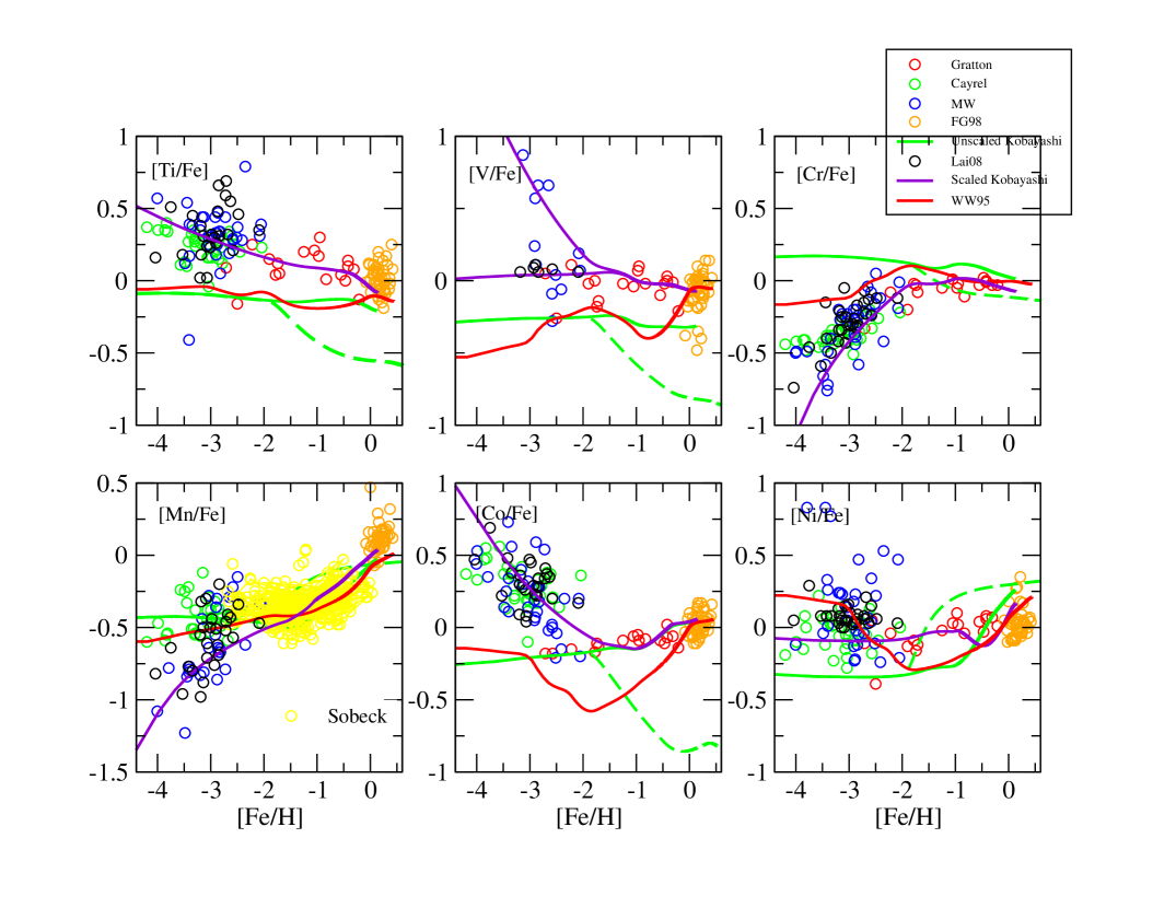
Figure 2: Like Fig. 1 but with model results included. The green tracks are from models which employ the original Fe-peak yields of Kobayashi et al. (2006), while the violet tracks are from models in which the scaled Kobayashi yields have been used. The red tracks refer to a model that employs the massive star Fe-peak yields of Woosley and Weaver (1995). The green dashed tracks show the results when details of the prescription of Matteucci et al. (2006) for SNIa events is employed. The legend shows the symbol and color for each data set of observed abundances.

Figure 2 shows the observed abundances in Fig. 1 but now with model tracks added. The solid green lines show the model results using the Kobayashi yields as published and unscaled. One can see that in the cases of Ti/Fe, V/Fe, Co/Fe, and perhaps Ni/Fe the model underpredicts the observed abundances, particularly at low metallicity. On the other hand, the same model predicts Cr/Fe levels above those observed but does well with Mn/Fe. In the case of V/Fe, the data are ambiguous, as it is unclear whether the ratio increases below [Fe]=-2, as indicated by a few of the McWilliam et al. (1995) points, or remains constant, as suggested by some data points from McWilliam et al. and Gratton and Sneden (1991).

In an alternative version of this model we employed the scheme for calculating the contributions of SNIa explosions discussed by Matteucci et al. (2006). This method, based upon empirical evidence, assumes the existence of a bimodal distribution of delay times, wherein 35-50% of the Type Ia progenitors have lifetimes around 10⁸ years, while the remaining systems involve small mass progenitors which require more time to evolve and have a broad distribution of delay times. This bimodal feature results in a significant number of Type Ia events beginning to occur at metallicities as low as [Fe/H]=-2.0, i.e., significantly earlier than the prescription of Matteucci & Greggio (1986) would predict. The result of using the Matteucci et al. (2006) scheme is shown with the dashed green line. Clearly there is no general improvement in the match between data and theory.

We note the significant scatter at low metallicity for most of the elements in Fig. 2, which makes interpretation of the trends more difficult. The possible explanations for this scatter include the lack of sufficient data, the presence of the ejecta from individual nucleosynthetic events such as the first stars, and insufficient mixing of that ejecta with the interstellar medium.

We next calculated a model using the massive star yields for Ti-Ni by Woosley and Weaver (1995), who listed isotope yields prior to decay. [Recall that François et al. (2004) used these yields in their analysis.] The isotopes whose individual yields contribute to the final yield for a particular Fe-peak element, either directly or through decay, are listed in Table 3. The solid red line shows the results in Fig. 2, and we point out that our tracks agree closely with the model results of Timmes et al. (1995), as expected. The quality of the match between observation and theory varies from element to element. For Ti/Fe, our computed track closely follows the one employing the Kobayashi et al. (2006) yields but neither reproduces the upward trend with declining metallicity. Roughly the same can be said for the case of V/Fe. For Cr/Fe our model reproduces the flat behavior of the data at metallicities above -2, but below that point the model has less of a downturn than the data. The model produces a good match with the data in the case of Mn/Fe, but falls well below the Co/Fe trends. Finally, in the case of Ni/Fe the WW95 model is consistent with the data at both the high and low metallicity ends, while sagging below the observations in the mid-range.

In order to improve the model fit to the observations and thus allow us to compute useful integrated yields, we applied scaling factors to the Kobayashi yields, thereby forcing a fit to the data. These factors were derived through trial and error and are listed in Table 4. In particular, for the Fe peak elements other than Fe itself, we adjusted the massive star yields in a succession of trial models until we obtained a reasonable eyeball fit to the data over the metallicity range from -4 $\rm<$ [Z] $\rm<$ +0.5. The model results in this case are shown in Fig. 2 with a solid violet line. We see that in the cases of Ti, V, Mn, and Co the trends are matched fairly well. We note that for V, a few of the points from the data of McWilliam et al. (1995) suggest an upward trend below a metallicity of -2. Thus, we used a second scaling factor to produce a model in which the behavior of those points in particular was reproduced. In the case of Ni, the scatter in the data below -2 is too large to speculate about the success of the model. Finally, the situation with Cr will be discussed further below as it relates to Co, but we simply point out here that while the apparent plateau below -3 is unexplained by our force fit model, the calculations employing either the Kobayashi et al. (2006) or Woosley and Weaver (1995) yields do produce a flattening in that low metallicity region.

We next derived the values for massive star integrated yields of the Fe-peak elements based upon our force fit model just described. We did this by rerunning the model incorporating the scaled Kobayashi yields and at each time (metallicity) point integrated the scaled yields over the same IMF as that used in the model calculations, i.e. a slightly flattened ($\rm\alpha$=-1.20) Salpeter IMF, according to equation 1. The integrated yields derived in this manner are provided in Table 5. Note that the integrated yields for V correspond to the upper model track.

The first two columns of the table give the log of the metallicity and its value normalized to the sun (Asplund et al., 2005), respectively, while subsequent columns list the log of the individual integrated yields. We emphasize that these integrated yields provide useful constraints for assessing published stellar yields, since any set of yields when integrated over an IMF should closely match them. Note that the IMF may have any form as long as the integral of the yields over that IMF gives the proper value for the integrated yield that is consistent with the observations.

The integrated scaled Kobayashi yields are plotted in Fig. 3 as a function of the log of metallicity (violet tracks) along with analogous values for the unscaled yields from the same authors (green tracks). (Since we did not use scaled Fe yields, only the unscaled integrated yield track is plotted for that element.) Clearly the largest offsets occur at metallicities below -2. In the cases of Ti, V, and Co, we find a clear decrease in the integrated yields as metallicity rises. This contrasts with the predictions of Kobayashi et al. (2006), who find relatively little metallicity sensitivity for the yields of these three elements. On the other hand, for Cr and Mn we infer a direct relation with metallicity for the yields of these elements, while again Kobayashi et al. (2006) find little metallicity effect. For Ni, our results are qualitatively similar to those of Kobayashi et al. (2006) below a metallicity of -1, after which we find that Ni yields decline while they infer a rise with increased metallicity. Quantitatively, the theoretical yields fall below our values at metallicities below solar.

While our general approach to yield evaluations resembles that of François et al. (2004), the details of the studies are different enough that a direct comparison of results is difficult if not impossible to make. For example, they scaled the yields of Woosley and Weaver (1995) for solar metallicity only, while we employed the Kobayashi et al. (2006) yields and accounted for metallicity effects. (Note that the latter set of yields was unavailable at the time of the François et al. study.) Obviously, a valid comparison would be possible only if the two research teams had based their studies on the same set of theoretical yields. We do point out, however, that both groups were successful at producing a model with scaled yields that resulted in good fits to the observations.

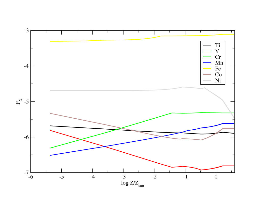
Figure 4: A comparison of integrated yields derived from the adjusted Kobayashi yields (the violet tracks in Fig. 3) for each of the seven Fe peak elements as a function of log Z/Z_⊙. The legend connects line color with the element. The value for Z_⊙ was assumed to be 0.0122 [Asplund et al. (2005).]

Finally, we compare our integrated yields from Table 5, of all seven of the Fe-peak elements we are considering, in Fig. 4 as a function of metallicity log Z. Here we see some interesting trends which we will attempt to interpret in the next section. First, Cr production increases while Co production decreases as a function of metallicity, resulting in the two tracks crossing at around log Z/Z_⊙ of -3. This result clearly is linked directly to the observed behavior of these two elements with metallicity (see data for these two elements in Fig. 1). Other interesting trends include the indirect behavior of V and Ti with metallicity.

Under conditions such as we have at low metallicity where the instantaneous recycling approximation applies, one can show using standard chemical evolution equations (Matteucci, 2001) that the only factors besides the integrated yields which might substantially influence the evolution of an element ratio are gas infall or outflow, through their diluting/concentrating effects. Therefore, we ran two variations of our force fit model in which we employed star formation time scales of 2 Gyr and 7 Gyr, where we previously used 4 Gyr in the basic model (see Table 2). We found no perceptible difference between the three models, suggesting that our integrated yield values are robust within a wide range of galaxy formation conditions and regions.

4 DISCUSSION

4.1 Abundance Ratios and Metallicity Trends

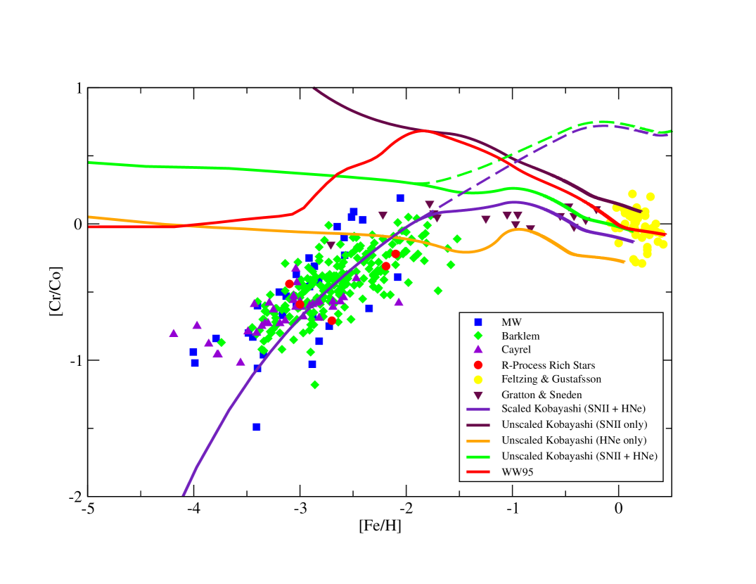
Figure 5: [Cr/Co] versus [Fe/H]. Data plotted are neutral species of the elements. Data sources are distinguished by symbol shape and color and are identified in the legend. Curves show the results of several chemical evolution models, also identified in the legend and explained in the text. The dashed green and violet lines show the effect of using the SNIa prescription of Matteucci et al. (2006) instead of that of Matteucci & Greggio (1986).

As discussed in the Introduction, the particular behavior of Cr/Co with increasing metallicity was originally pointed out by McWilliam et al. (1995) and deserves special attention. This behavior is illustrated in Fig. 5, where to the data displayed in Figs. 1 and 2 we have added abundances from Barklem et al. (2005) indicated with green diamonds. Also shown in the figure are five well-studied r-process-rich halo stars, indicated by red circles. The abundance ratios of Cr/Co in all of these high-resolution, high S/N studies (CS 22892-052, [Fe/H] = –3.1, Sneden et al. (2003); HD 115444, [Fe/H] = –3.0, Westin et al. (2000); HD 122563, [Fe/H] = –2.7, Westin et al. (2000); BD+17 3248, [Fe/H] = –2.1, Cowan et al. (2002); HD 221170, [Fe/H] = –2.2, Ivans et al. (2006)) are consistent with the behavior of the other sample stars illustrated here.

The data together show a steady increase by a factor of more than 10 in Cr/Co between -4 and -1.5 of [Fe/H], followed by a leveling off at roughly -1.5 as metallicity continues to increase. For comparison, data presented in Timmes et al. (1995), which extend down only to -3 in metallicity, show a slight decline in Cr/Fe, while Co/Fe remains level at their lowest metallicities, although the scatter is enough that it is difficult to discern a downward trend in Cr/Co [Timmes et al. (1995) do not explicitly plot Cr/Co].

In Fig. 5 we also show the predictions of several chemical evolution models, where the line types and colors are consistent with those used in Fig. 2. Here we see that the model which employed the scaled Kobayashi yields and successfully matched the Cr and Co trends with Fe in Fig. 2 satisfactorily reproduces the trend in Cr/Co in Fig. 5 (solid violet track), as expected. This is true at least out to -3.5 in metallicity, below which the data suggest the presence of a plateau, which is not predicted by our model. The model using the Kobayashi yields as published (solid green track), along with two variations of it in which all core collapse events are either SNII (solid maroon track) or hypernovae (solid orange track), are generally consistent with the data above a metallicity of -2 but fail to reproduce the downward trend at lower metallicities. Also, models in which the SNIa scheme of Matteucci et al. (2006) was used are indicated with dashed lines of the same color as the associated model that makes use of the same stellar yields and input parameters. Clearly, this change does not produce an improvement to the original models. Finally, the solid red line represents the model in which we employed the yields and input parameters of Woosley and Weaver (1995) and Timmes et al. (1995), respectively. This track does not match the data well except near solar metallicities, due in large part to the predicted behavior of Co/Fe (see Fig. 2).

In general, the yields of Kobayashi et al. (2006) coupled with either an equal mix of SNII and hypernovae or 100% hypernovae give reasonable matches to the data at metallicities above -1.5. At metallicities below this, however, the nearly level predicted values of Cr/Co for these two models fail to match the downward trend. Also, the all-SNII model predicts Cr/Co values which are generally too high at all metallicities.

An additional comment concerns the apparent plateau below about -3.5 in metallicity. Clearly, our forced fit using scaled Kobayashi yields does not reproduce this behavior. At the same time, however, we note that the model using the WW95 yields does predict a roughly constant value for [Cr/Co] over this metallicity range. Combining the WW95 results below -3 with the scaled Kobayashi model results above that level would clearly produce a good fit to the data.

Finally, we see that the general upward trend of [Cr/Co] with metallicity for [Fe/H] below -1.5 in Fig. 5 is explained by increasing Cr integrated yields and decreasing Co integrated yields below [Z]=-1.2 in Fig. 4. Above that same point, while Cr yields appear to level off, the Co yields actually reverse direction and go up. According to the discussion in Nakamura et al. (1999), the behavior of Cr and Co yields below -1.2 may be linked to a systematic outward migration of the mass cut with metallicity during the SN explosion.

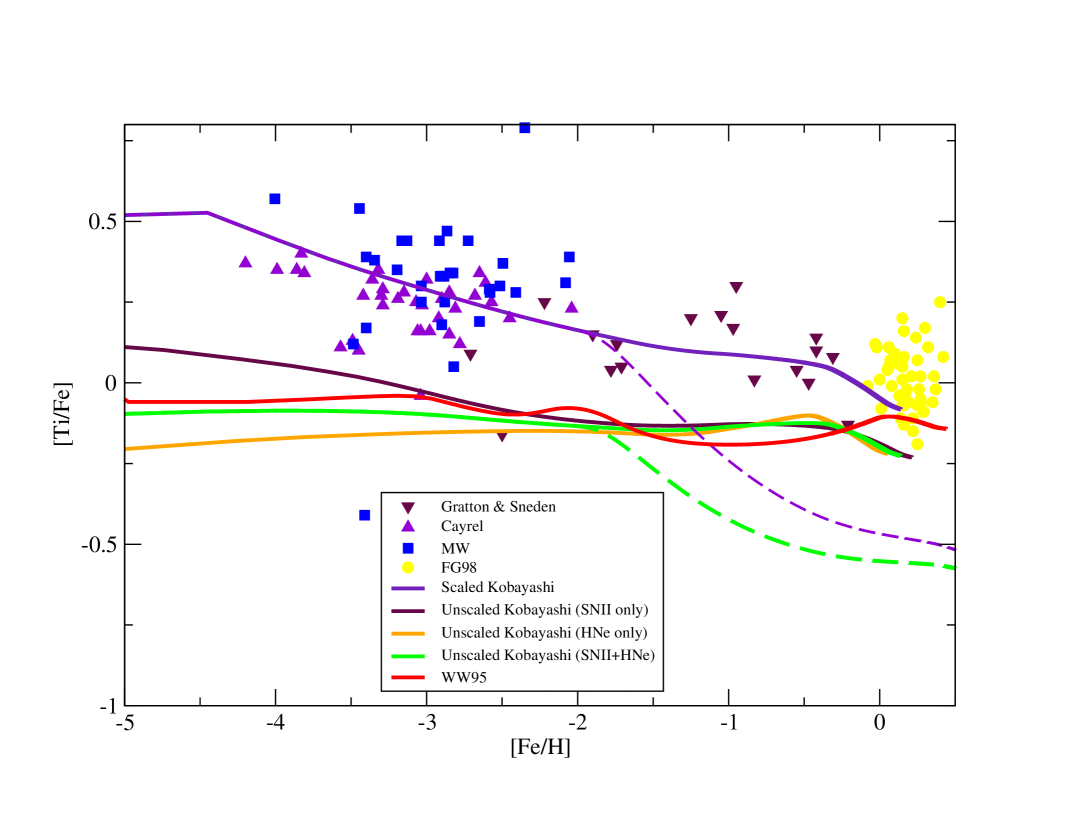
Figure 6: Like Fig. 5 but for [Ti/Fe] versus [Fe/H]. Data sources are distinguished by symbol shape and color and are identified in the legend. Curves show the results of several chemical evolution models, also identified in the legend and explained in the text. The dashed green and violet lines show the effect of using the SNIa prescription of Matteucci et al. (2006) instead of that of Matteucci & Greggio (1986).

The same models featured in the above analysis of [Cr/Co] are shown in Fig. 6, which displays the data and models relevant to [Ti/Fe]. Again we see that the scaled Kobayashi model successfully reproduces the trend in the data, while the others are less successful. In particular, the model employing the Woosley and Weaver (1995) yields (solid red track) fails by two orders of magnitude to reproduce the [Ti/Fe] behavior. Referring again to Fig. 4 we see that the observed downward trend in [Ti/Fe] is consistent with a similar trend in the integrated yield of Ti.

4.2 Recent Findings for Cr and Co

There have been two recent laboratory determinations of atomic data (e.g. oscillator strengths) for both the neutral (Sobeck et al. 2007) and first-ionized species (Nilsson et al. 2006) of chromium. The study by Lai et al. (2008) was the only one of our selected sample to employ these new data. They found that [CrI/Fe] ratio decreased in the region -4.3 $\rm\leq$ [Fe/H] $\rm\leq$ -2.0 while the [CrII/Fe] ratio remained solar over the same metallicity range. As a follow-up, they generated plots of Cr I and Cr II as a function of effective temperature (T_eff; a stellar atmospheric parameter) and discovered a trend in the Cr I data. Their finding may indicate that the neutral Cr abundances are affected by departures from LTE.

Similarly, there have been up-to-date laboratory determinations of oscillator strengths for both the neutral (Nitz et al. 1999) and first-ionized species (Crespo Lopez Urratia et al. 1994) of cobalt. The abundance investigation of 17 stars by Bergemann (2008), which employed a non-LTE methodology and these new atomic data, found that the [CoI/Fe] ratio increases as metallicity decreases in the range -2.5 $\rm\leq$ [Fe/H] $\rm\leq$ 0.0. This result contradicts the data from our selected studies and signifies that Co I abundances are susceptible to non-LTE effects. It is evident that further examination of both the Cr and Co abundance trends with [Fe/H] over the full extent of metallicity and in a statistically-significant data sample is warranted to validate these two recent findings.

4.3 Supernova Nucleosynthesis Explanations

As discussed above and indicated by red, filled circles in Fig. 5, we included five well-studied, metal-poor r-process-rich stars in our abundance comparisons of Cr/Co. Since the suggested site for the r-process is core-collapse (massive star) supernovae (see e.g., Sneden, Cowan, & Gallino 2008), the products of (early Galactic) nucleosynthesis in these halo stars, including the iron-peak elements, have not had major contributions from Type Ia SNe - those events presumably arising from objects that require much longer stellar evolutionary timescales than Type II SNe. There have been several attempts to explain the behavior of Cr/Co versus metallicity based upon Type II supernova nucleosynthesis. Thus, for example it has been shown that Co and Fe result from complete Si burning, while Cr is synthesized in these models from incomplete Si burning (Nakamura et al. 1999). We see in Fig. 1 that [Co/Fe] and [Cr/Fe] have opposite slopes with respect to metallicity.

We note that the results of Nakamura et al. supernova models depend critically upon the mass cuts between the nascent neutron star (or black hole) and the ejected envelope. The yields of the synthesized material depends upon the ejected mass, and thus directly upon these mass cuts. How these mass cuts depend upon progenitor masses and upon the explosion energies is also critical to determining the elemental yields. In addition there may be other contributing factors in these models such as rotation energy that could affect the nucleosynthesis products.

4.4 Ionization States, Atomic Data and Abundances

The selected abundance investigations do have a few weak points. For instance, they do not employ the most recent determinations of atomic data (with exception of V I, V II, and Fe I). Additionally, there is a general presumption of iron as a reliable and robust abundance indicator. However recently, Lai et al. (2008) found a correlation between excitation potential and both metallicity and effective temperature for Fe I transitions (in a sample of extremely metal deficient stars). As an alternative, Kraft & Ivans (2004) suggest the exclusive employment of Fe II transitions to derive metallicity (and thereby, avoid the issues associated with the use of Fe I lines). None of the chosen investigations did this in their respective determinations of metallicity.

Also for the majority of stars examined (with low temperature and metallicity), the dominant form of all of the elements is the first-ionized species (especially the elements with an ionization potential less than 7 eV: Ti, V, Cr). Yet, the selected studies largely rely upon transitions only from the neutral species of the element (and in fact, do not present any data for Mn II or Co II).

Then, the derivation of abundances from Fe-peak elements is sensitive to departures from LTE (effects such as overionization and resonance scattering; e.g. Shchukina & Trujillo Bueno 2001). For example, the abundance investigation of 14 stars by Bergemann & Gehren (2008), which employed a non-LTE methodology, found that the [MnI/Fe] ratio remained solar in a metallicity range -2.5 $\rm\leq$ [Fe/H] $\rm\leq$ 0.0. This finding contradicts the results of the selected abundance studies. Note though, that the magnitude of these non-LTE effects (for each of the elements) has yet to be quantified in rigorous and consistent analysis of a large stellar sample.

5 SUMMARY & CONCLUSIONS

The principal goal of this paper has been to produce a set of integrated stellar yields which can be used by theorists in the future to test their yield predictions for Fe-peak elements. Utilizing an extensive data base of published stellar iron peak elemental abundances for the solar vicinity, we have produced plots of the form [X/Fe] versus [Fe/H] for the elements Ti, V, Cr, Mn, Co, and Ni. We next employed detailed one-zone chemical evolution models to evaluate the massive star yields of Woosley and Weaver (1995) and Kobayashi et al. (2006) in their ability to reproduce these trends. Finally, we scaled the latter yield set and used it as input to our models in order to force a fit to the data for each plot. From this scaled set we then derived our empirical integrated yields, using a slightly flattened time-independent Salpeter initial mass function. Our analysis led to the following conclusions:

• As recognized previously by other authors, there are clear upward trends of [Ti/Fe] and [Co/Fe] and downward trends of [Co/Fe] and [Mn/Fe] as metallicity decreases. This is especially the case below [Fe/H] of roughly -2.

• The above trends appear to be the result of changes in massive star yields with metallicity and are unrelated to star formation history.

• Models utilizing yields of Kobayashi et al. (2006) and Woosley and Weaver (1995) generally reproduce the data near solar metallicity. However, the agreement between observation and theory at lower metallicities is generally less satisfactory.

• A set of integrated yields as a function of metallicity was derived from global data trends for six elements.

In applying scaling factors to the yields of Kobayashi et al. (2006) to force a fit to the observations, we make the following comparisons between the empirical and theoretical yields. Our results suggest that actual yields of Ti, V, and Co are generally larger as well as anticorrelated with metallicity compared to the Kobayashi et al. (2006) predictions. We also find the yields of Cr and Mn to be generally smaller and directly correlated with metallicity compared to the theoretical results. Our results for Ni are consistent with theory, although our model suggests that all Ni yields should be scaled up slightly.

One clear problem with our analysis involves the scatter in the data and in some cases the difficulty in establishing the nature or direction of the trend. A good example can be seen in the plot of [V/Fe] versus [Fe/H] in Fig. 1, where we see both a possible flat as well as an upward trend below [Fe/H]=-2. A second example appears in the graph of [Cr/Fe] versus [Fe/H] at metallicities below -3. Here we see an apparent bifurcation in the data as one branch remains horizontal while the other continues trending downward. In the case of V, we have attempted to match both branches, while in the Cr case we ignore the horizontal branch for now. At these low metallicities it is likely that the abundance pattern observed in a star is the result of expelled material from only one earlier-generation star instead of a well-mixed contribution from many such stars. Thus, star to star variations echo analogous differences in the yields of the earlier stars. This is not an effect which our models are designed to take into account. Rather homogeneous mixing is assumed. Future work should attempt to explore the causes of the observed scatter and its possible link to apparent bifurcations in the data. For now we have attempted only to analyze what we see as global trends in each plot in Fig. 1.

Table 1: Observational Characteristics of the Selected Abundance Analyses

Study	Telescope/Instrument	Program Stars	Wavelength Coverage Region [Å]	S/N Range	Resolution	Metallicity Range	Species Detected
Gratton $\rm\&$ Sneden 1991	CAT/CES	19	4122-6434	150	50000	-2.7$\rm<$[Fe/H]$\rm<$-0.2	Ti I/II;V I/II;Cr I/II;Mn I;Fe I/II;Co I;Ni I
McWilliam et al. 1995	LCO/echelle	33	3600-7600	12-47	22000	-4.1$\rm<$[Fe/H]$\rm<$-1.9	Ti I/II;V I/II;Cr I;Mn I;Fe I/II;Co I;Ni I
Feltzing $\rm\&$ Gustafsson 1998	McD/2-d coudé	47	3900-7000	200	100000	-0.1$\rm<$[Fe/H]$\rm<$+0.5	Ti I;V I/II;Cr I/II;Mn I;Fe I/II;Co I;Ni I
Cayrel et al. 2004	VLT/UVES	70	3300-10000	95-430	45000	-4.1$\rm<$[Fe/H]$\rm<$-2.7	Ti I/II;Cr I;Mn I;Fe I/II;Co I;Ni I
Sobeck et al. 2006	McD/2-d coudé; Keck/HIRES	216	6010-6025	40-240	40000-60000	-2.7$\rm<$[Fe/H]$\rm<$+0.1	Mn I
Lai et al. 2008	Keck/HIRES	28	3020-7665	8-425	40000	-4.2$\rm<$[Fe/H]$\rm<$-2.6	Ti I/II;V I/II;Cr I/II;Mn I/II;Fe I/II;Co I;Ni I

Table 2: Basic Input Parameters for Chemical Evolution Models

Parameter	Value
Star Formation Efficiency	2.8 Gyr-1
Star Formation Power Law Exponent	1.5
Initial Mass Function Exponent, $\rm\alpha$	-1.20
Stellar Mass Range Lower Limit	0.08 M⊙
Stellar Mass Range Upper Limit	40 M⊙
Infall Time Scale	4 Gyr
Current Total Mass Density	50 M⊙ pc-2
Current Age	13 Gyr
Type Ia Factor, c	0.007
Hypernova Fraction, $\rm\epsilon$	0.5

Table 3: WW95 Yields: Isotopes Contributing to Stable Element

Element	Isotopes
Ti	46Ti, 47Ti, 48Ti, 49Ti, 50Ti, 47V, 48V, 49V, 48Cr, 49Cr
V	50V, 51V, 51Cr, 51Mn
Cr	50Cr, 52Cr, 53Cr, 54Cr, 52Mn, 53Mn, 54Mn, 52Fe
Mn	55Mn, 55Fe, 55Co
Fe	54Fe, 56Fe, 57Fe, 58Fe, 56Co, 57Co, 58Co, 56Ni
Co	59Fe, 59Co, 59Ni, 59Cu
Ni	60Co, 61Co, 58Ni, 60Ni, 61Ni, 62Ni, 64Ni, 60Cu

Table 4: Scaling Factors for the Kobyashi et al. Yields

Element	[Fe/H] Range	Scaling Factor
Ti	full range	0.15-0.063x
V	x$\rm\leq$-2	-0.34-0.32x
V	x$\rm>$-2	+0.30
Cr	x$\rm\leq$-2	+0.50+0.30x
Cr	x$\rm>$-2	-0.10
Mn	x$\rm\leq$-1.5	+0.36+0.18x
Mn	x$\rm>$-1.5	+0.10
Co	x$\rm\leq$-1.75	-0.39-0.89x
Co	x$\rm>$-1.75	0.0
Ni	x$\rm\leq$-1.0	-0.75-x
Ni	x$\rm>$-1.0	+0.25

Table 5: Integrated Yields

$\rm\log Z$	[Z]	$\rm\log P_{Ti}$	$\rm\log P_{V}$	$\rm\log P_{Cr}$	$\rm\log P_{Mn}$	$\rm\log P_{Fe}$	$\rm\log P_{Co}$	$\rm\log P_{Ni}$
-$\rm\infty$	-$\rm\infty$	-5.70	-5.83	-6.32	-6.52	-3.32	-5.34	-4.69
-6.0	-4.3	-5.76	-6.14	-6.03	-6.34	-3.30	-5.58	-4.71
-4.0	-2.3	-5.86	-6.67	-5.51	-6.04	-3.23	-5.94	-4.69
-3.0	-1.3	-5.89	-6.83	-5.32	-5.87	-3.15	-6.05	-4.61
-2.0	-0.3	-5.91	-5.83	-5.33	-5.70	-3.12	-5.95	-4.76
-1.7	0.0	-5.88	-6.83	-5.32	-5.62	-3.13	-5.78	-4.96
-1.3	+0.4	-5.88	-6.82	-5.31	-5.61	-3.11	-5.76	-5.44

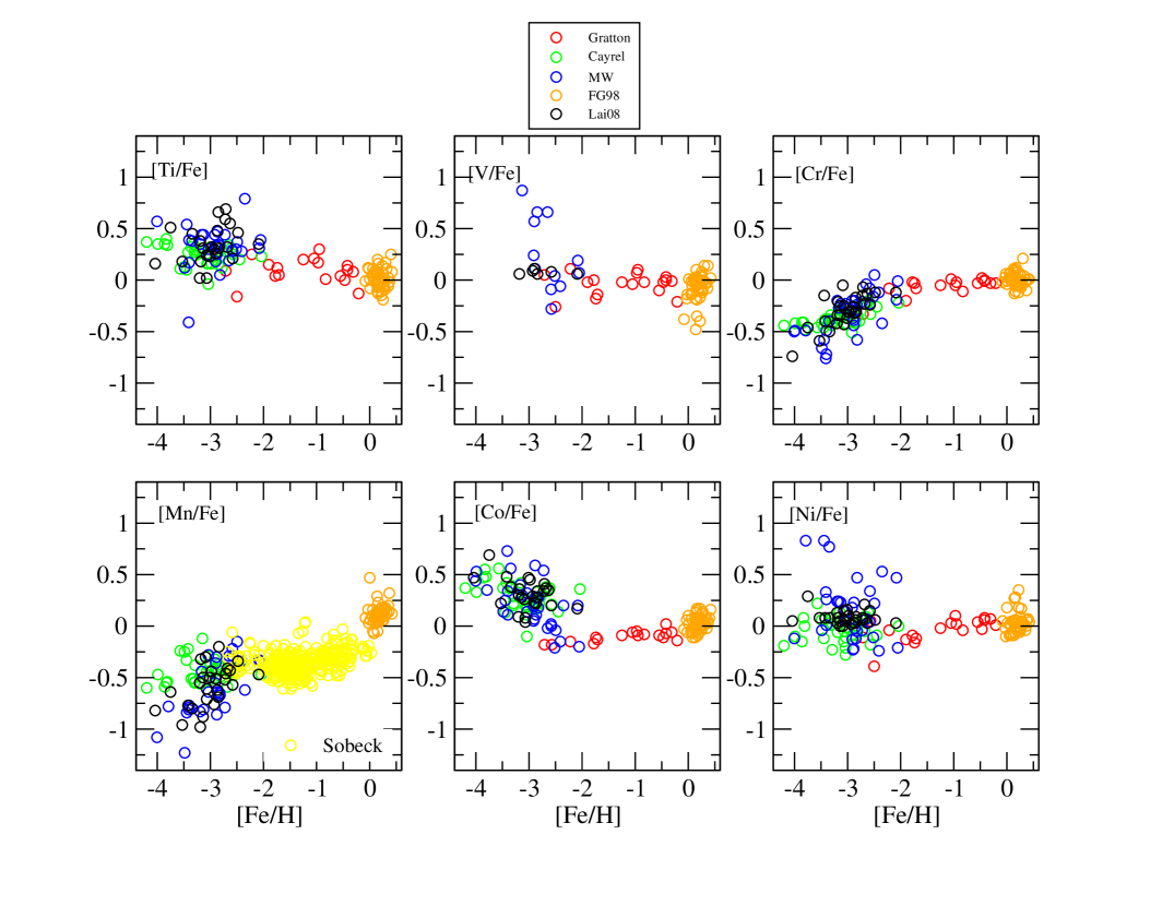
Figure 1: Plots of [X/Fe] versus [Fe/H], showing observed values published in those sources indicated by symbol color defined in the legend. The specific ratio representing the dependent variable is indicated in the upper left corner of each panel.

Figure 3: The integrated yield P_x versus log Z/Z_⊙ for the seven elements of the Fe peak under consideration. Green tracks refer to unadjusted yields from Kobayashi et al. (2006), while violet tracks show values for the adjusted yields. The value for Z_⊙ was assumed to be 0.0122 [Asplund et al. (2005).]

References

- Asplund et al. (2005) Asplund, M., Grevesse, N., & Sauval, A.J. 2005, in Cosmic Abundances as Records of Stellar Evolution and Nucleosynthesis, ASP Conf. Ser. 30, F.N. Bash & T.G. Barnes, eds.
- Barklem et al. (2005) Barklem, P.S., Christlieb, N., Beers, T.C., Hill, V., Bessell, M.S., Holmberg, J., Marsteller, B., Rossi, S., Zickgraf, F.-J., & Reimers, D. 2005, A&A, 439, 129
- Bergemann & Gehren (2008) Bergemann & Gehren 2008, A&A, 492, 823
- Bergemann et al. (2008) Bergemann 2008, Phys. Scr., T133
- Cayrel et al. (2004) Cayrel, R., Depagne, E., Spite, M., Hill, V., Spite, F., François, P., Plez, B., Beers, T., Primas, F., Andersen, J., Barbuy, B., Bonifacio, P., Molaro, P., & Nordström, B. 2004, A&A, 416, 1117
- Chiappini et al. (1997) Chiappini, C., Matteucci, F., & Gratton, R. 1997, ApJ. 477, 765
- Cowan et al. (2002) Cowan, J. J., et al. 2002, ApJ, 572, 861
- Crespo et al. (1994) Crespo Lopez-Urrutia, J.R., Neger, T., and Jager, H. 1994, J Phys D, 27, 994