Modelling Clock Synchronization in the Chess gMAC WSN Protocol

Abstract

We present a detailled timed automata model of the clock synchronization algorithm that is currently being used in a wireless sensor network (WSN) that has been developed by the Dutch company Chess. Using the Uppaal  model checker, we establish that in certain cases a static, fully synchronized network may eventually become unsynchronized if the current algorithm is used, even in a setting with infinitesimal clock drifts.

1 Introduction

Wireless sensor networks consist of autonomous devices that communicate via radio and use sensors to cooperatively monitor physical or environmental conditions. In this paper, we formally model and analyze a distributed algorithm for clock synchronization in wireless sensor networks that has been developed by the Dutch company Chess in the context of the MyriaNed project [16]. Figure 1 displays a sensor node developed by Chess.

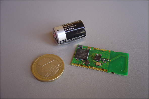
Figure 1: Chess MyriaNode 2.4 Ghz wireless sensor node

The algorithm that we consider is part of the Medium Access Control (MAC) layer, which is responsible for the access to the wireless shared channel. Within its so-called gMAC protocol, Chess uses a Time Division Multiple Access (TDMA) protocol. Time is divided in fixed length frames, and each frame is subdivided into slots (see Figure 2).

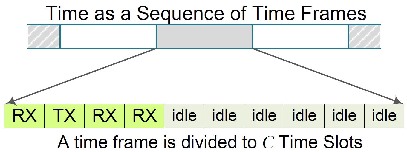
Figure 2: The structure of a time frame

Slots can be either active or sleeping (idle). During active slots, a node is either listening for incoming messages from neighboring nodes (RX) or it is sending a message (TX). During sleeping slots a node is switched to energy saving mode. Since energy efficiency is a major concern in the design of wireless sensor networks, the number of active slots is typically much smaller than the total number of slots (less than $1\%$ in the current implementation). The active slots are placed in one contiguous sequence which currently is placed at the beginning of the frame. A node can only transmit a single message per time frame, during its TX slot. The protocol takes care that neighboring nodes have different TX slots.

One of the greatest challenges in the design of the MAC layer is to find suitable mechanisms for clock synchronization: we must ensure that whenever some node is sending all its neighbors are listening. Sensor nodes come equipped with a crystal clock, which may drift. This may cause the TDMA time slot boundaries to drift and thus lead to situations in which nodes get out of sync. To overcome this problem nodes will have to adjust their clocks now and then. Also, the notion of guard time is introduced: at the beginning of its TX slot, a sender waits a certain amount of time to ensure that all its neighbors are ready to receive messages. Similarly, a sender does not transmit for a certain amount of time at the end of its TX slot. In order to save energy it is important to reduce these guard times to a minimum. Many clock synchronization protocols have been proposed for wireless sensor networks, see e.g.  [17, 6, 18, 13, 2, 12, 15]. However, these protocols (with the exception of [18, 2] and possibly [15]) involve a computation and/or communication overhead that is unacceptable given the extremely limited resources (energy, memory, clock cycles) available within the Chess nodes.

To experiment with its designs, Chess currently builds prototypes and uses advanced simulation tools. However, due to the huge number of possible network topologies and clock speeds of nodes, it is difficult to discover flaws in the clock synchronization algorithm via these methods. Timed automata model checking has been succesfully used for the analysis of worst case scenarios for protocols that involve clock synchronization, see for instance [5, 9, 20]. To enable model checking, models need to be much more abstract than for simulation, and also the size of networks that can be tackled is much smaller, but the big advantage is that the full state space of the model can be explored.

In this paper, we present a detailed model of the Chess gMAC algorithm using the input language of the timed automata model checking tool Uppaal  [4]. Another Uppaal  model for the gMAC algorithm is presented in [10], but that model deviates and abstracts from several aspects in the implementation in order to make verification feasible. The aim of the present paper is to construct a model that comes as close as possible to the specification of the clock synchronization algorithm presented in [16]. Nevertheless, our model still does not incorporate some features of the full algorithm and network, such as dynamic slot allocation, synchronization messages, uncertain communication delays, and unreliable radio communication. At places where the informal specification of [16] was incomplete or ambiguous, the engineers from Chess kindly provided us with additional information on the way these issues are resolved in the current implementation of the network [21]. In the current implementation of Chess, a node can only adjust its clock once every time frame during the sleeping period, using an extension of the Median algorithm of [18]. This contrasts with the approach in [10] in which a sensor node may adjust its clock after every received message. In the present paper we faithfully model the Median algorithm as implemented by Chess. Another feature of the gMAC algorithm that was not addressed in [10] but that we model in this paper is the radio switching time: there is some time involved in the transition from sending mode to receiving mode (and vice versa), which in some cases may affect the correctness of the algorithm.

The Median algorithm works reasonably well in practice, but by means of simulation experiments, Assegei [2] already exposed some flaws in the algorithm: in some test cases where new nodes join or networks merge, the algorithm fails to converge or nodes may stay out of sync for a certain period of time. Our analysis with Uppaal  confirms these results. In fact, we show that the situation is even worse: in certain cases a static, fully synchronized network may eventually become unsynchronized if the Median algorithm is used, even in a setting with infinitesimal clock drifts.

In Section 2, we explain the gMAC algorithm in more detail. Section 3 describes our Uppaal  model of gMAC. In Section 4, the analysis results are described. Finally, in Section 5, we draw some conclusions. In this paper, we assume that the reader has some basic knowledge of the timed automaton tool Uppaal. For a detailed account of Uppaal, we refer to [4, 3] and to http://www.uppaal.com. The Uppaal model described in this paper is available at http://www.mbsd.cs.ru.nl/publications/papers/fvaan/chess09/.

2 The gMAC Protocol

In this section we provide additional details about the gMAC protocol as it has currently been implemented by Chess.

2.1 The Synchronization Algorithm

In each frame, each node broadcasts one message to its neighbors. The timing of this message is used for synchronization purposes: a receiver may estimate the clock value of a sender based on the time when the message is received. Thus there is no need to send around (logical) clock values. In the current implementation of Chess, clock synchronization is performed once per frame using the following algorithm [2, 21]:

1. In its sending slot, a node broadcasts a packet which contains its transmission slot number.

2. Whenever a node receives a message it computes the phase error, that is the difference (number of clock cycles) between the expected receiving time and the actual receiving time of the incoming message. Note that the difference between the sender’s sending slot number (which is also the current slot number of the sender) and the current slot number of the receiving node must also be taken into account when calculating the phase errors.

3. After the last active slot of each frame, a node calculates the offset from the phase errors of all incoming messages in this frame with the following algorithm:

        if (number of received messages == 0)
                 offset = 0;
        else if (number of received messages <= 2)
                 offset = the phase error of the first received message * gain;
        else
                 offset = the median of all phase errors * gain
   

   Here gain is a coefficient with value 0.5, used to prevent oscillation of the clock adjustment.

4. During the sleeping period, the local clock of each node is adjusted by the computed offset obtained from step 3.

In situations when two networks join, it is possible that the phases of these networks differ so much that the nodes in one network are in active slots whereas the nodes in the other network are in sleeping slots and vice versa. In this case, no messages can be exchanged between two networks. Therefore in the Chess design, a node will send an extra message in one (randomly selected) sleeping slot to increase the chance that networks can communicate and synchronize with each other. This slot is called the synchronization slot and the message is in the same format as in the transmission slot. The extreme value of offset can be obtained when two networks join: it may occur that the offset is larger than half the total number of clock cycles of sleeping slots in a frame. Chess uses another algorithm called join to handle this extreme case. We decided not to model joining of networks and synchronization messages because currently we do not have enough information about the join algorithm.

2.2 Guard Time

The correctness condition for gMAC that we would like to establish is that whenever a node is sending all its neighbors are in receiving mode. However, at the moment when a node enters its TX slot we cannot guarantee, due to the phase errors, that its neighbors have entered the corresponding RX slot. This problem is illustrated in Figure 3 (a). Given two nodes 1 and 2, if a message is transmitted during the entire sending slot of node 1 then this message may not be successfully received by node 2 because of the imperfect slot alignment. Taking the clock of node 1 as a reference, the clock of node 2 may drift backwards or forwards. In this situation, node 1 and node 2 may have a different view of the current slot number within the time interval where node 1 is sending a message.

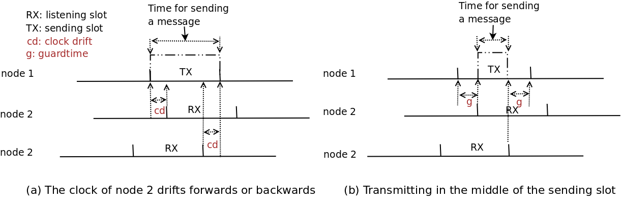
Figure 3: The need for introducing guard times

To cope with this problem, messages are not transmitted during the entire sending slot but only in the middle, as illustrated in Figure 3 (b). Both at the beginning and at the end of its sending slot, node 1 does not transmit for a preset period of ${\sf g}$ clock ticks, in order to accomodate the forwards and backwards clock drift of node 2. Therefore, the time available for transmission equals the total length of the slot minus $2{\sf g}$ clock ticks.

2.3 Radio Switching Time

The radio of a wireless sensor node can either be in sending mode, or in receiving mode, or in idle mode. Switching from one mode to another takes time. In the current implementation of the Chess gMAC protocol, the radio switching time is around $130\mu$sec. The time between clock ticks is around $30\mu$sec and the guard time ${\sf g}$ is $9$ clock ticks. Hence, in the current implementation the radio switching time is smaller than the guard time, but this may change in future implementations. If the first slot in a frame is an RX slot, then the radio is switched to receiving mode some time before the start of the frame to ensure that the radio will receive during the full first slot. However if there is an RX slot after the TX slot then, in order to keep the implementation simple, the radio is switched to the receiving mode only at the start of the RX slot. Therefore messages arriving in such receiving slots may not be fully received. This issue may also affect the performance of the synchronization algorithm.

3 Uppaal Model

In this section, we describe the Uppaal  model that we constructed of the gMAC protocol.

We assume a finite, fixed set of wireless nodes ${\sf Nodes}=\{0,\ldots,{\sf N}-1\}$. The behavior of an individual node ${\sf id}\in{\sf Nodes}$ is described by five timed automata ${\sf Clock}({\sf id})$, ${\sf Receiver}({\sf id})$, ${\sf Sender}({\sf id})$, ${\sf Synchronizer}({\sf id})$ and ${\sf Controller}({\sf id})$. Figure 4 shows how these automata are interrelated. All components interact with the clock, although this is not shown in Figure 4. Automaton ${\sf Clock}({\sf id})$ models the hardware clock of node ${\sf id}$, automaton ${\sf Sender}({\sf id})$ the sending of messages by the radio, automaton ${\sf Receiver}({\sf id})$ the receiving part of the radio, automaton ${\sf Synchronizer}({\sf id})$ the synchronization of the hardware clock, and automaton ${\sf Controller}({\sf id})$ the control of the radio and the clock synchronization.

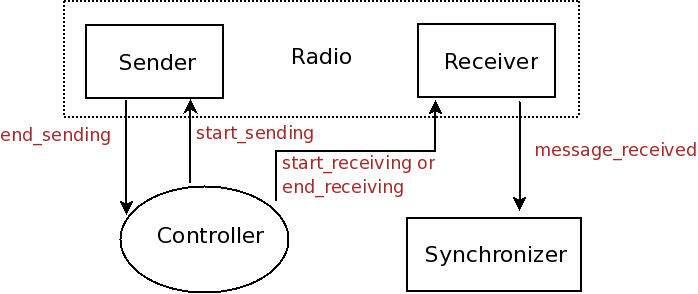
Figure 4: Message flow in the model

Table 1 lists the parameters that are used in the model (constants in Uppaal terminology), together with some basic constraints. The domain of all parameters is the set of natural numbers. We will now describe the five automaton templates used in our model.

Parameter	Description	Constraints
${\sf N}$	number of nodes	$0<{\sf N}$
${\sf C}$	number of slots in a time frame	$0<{\sf C}$
${\sf n}$	number of active slots in a time frame	$0<{\sf n}\leq{\sf C}$
${\sf tsn}[{\sf id}]$	TX slot number for node ${\sf id}$	$0\leq{\sf tsn}[{\sf id}]<{\sf n}$
${\sf k_{0}}$	number of clock ticks in a time slot	$0<{\sf k_{0}}$
${\sf g}$	guard time	$0<{\sf g}$
${\sf r}$	radio switch time	$0\leq{\sf r}$
${\sf min}[{\sf id}]$	minimal time between two clock ticks of node ${\sf id}$	$0<{\sf min}[{\sf id}]$
${\sf max}[{\sf id}]$	maximal time between two clock ticks of node ${\sf id}$	${\sf min}[{\sf id}]\leq{\sf max}[{\sf id}]$

Table 1: Protocol parameters

Clock

Timed automaton ${\sf Clock}({\sf id})$ models the behavior of the hardware clock of node ${\sf id}$. The automaton is shown in Figure 5. At the start of the system state variable ${\sf csn}[{\sf id}]$, that records the current slot number, is initialized to ${\sf C}-1$, that is, to the last sleeping slot. Hardware clocks are not perfect and so we assume a minimal time $\min[{\sf id}]$ and a maximal time $\max[{\sf id}]$ between successive clock ticks. Integer variable ${\sf clk}[{\sf id}]$ records the current value of the hardware clock. For convenience (and to reduce the size of the state space), we assume that the hardware clock is reset at the end of each slot, that is after ${\sf k_{0}}$ clock ticks. Also, a state variable ${\sf csn}[{\sf id}]$, which records the current slot number of node ${\sf id}$, is updated each time at the start of a new slot.

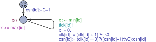
Figure 5: Automaton ${\sf Clock}[{\sf id}]$

Sender

The sending behavior of the radio is described by the automaton ${\sf Sender}[{\sf id}]$ shown in Figure 6.

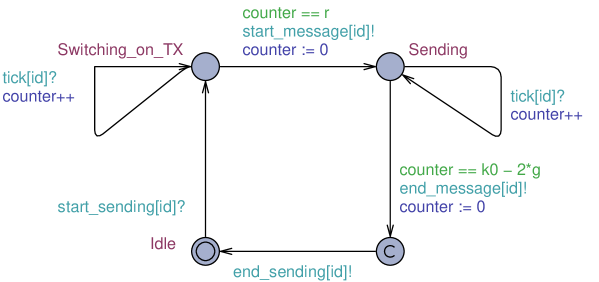
Figure 6: Automaton ${\sf Sender}[{\sf id}]$

The behavior is rather simple. When the controller asks the sender to transmit a message (via a $\sf start\_sending[{\sf id}]$ signal), the radio first switches to sending mode (this takes ${\sf r}$ clock ticks) and then transmits the message (this takes ${\sf k_{0}}-2\cdot{\sf g}$ ticks). Immediately after the message transmission has been completed, an $\sf end\_sending[{\sf id}]$ signal is sent to the controller to indicate that the message has been sent.

Receiver

The automaton ${\sf Receiver}[{\sf id}]$ models the receiving behavior of the radio. The automaton is shown in Figure 7. Again the behavior is rather simple. When the controller asks the receiver to start receiving, the receiver first switches to receiving mode (this takes ${\sf r}$ ticks). After that, the receiver may receive messages from all its neighbors. A function $\sf neighbor$ is used to encode the topology of the network: $\sf neighbor(j,id)$ holds if messages sent by $\sf j$ can be received by ${\sf id}$. Whenever the receiver detects the end of a message transmission by one of its neighbors, it immediately informs the synchronizer via a $\sf message\_received[{\sf id}]$ signal. At any moment, the controller can switch off the receiver via an $\sf end\_receiving[{\sf id}]$ signal.

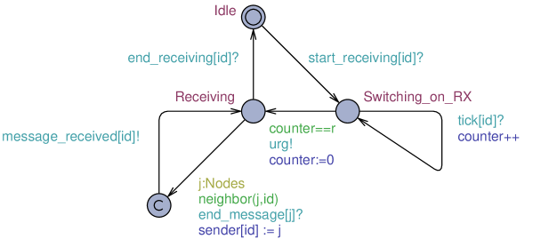
Figure 7: Automaton ${\sf Receiver}[{\sf id}]$

Controller

The task of the ${\sf Controller}[{\sf id}]$ automaton, displayed in Figure 9, is to put the radio in sending and receiving mode at the appropriate moments. Figure 9 shows the definition of the predicates used in this automaton. The radio should be put in sending mode ${\sf r}$ ticks before message transmission starts (at time ${\sf g}$ in the transmission slot of ${\sf id}$). If ${\sf r}>{\sf g}$ then the sender needs to be activated ${\sf r}-{\sf g}$ ticks before the end of the slot that precedes the transmission slot. Otherwise, the sender must be activated at tick ${\sf g}-{\sf r}$ of the transmission slot. If the first slot in a frame is an RX slot, then the radio is switched to receiving mode ${\sf r}$ time units before the start of the frame to ensure that the radio will receive during the full first slot. However if there is an RX slot after the TX slot then, as described in Section 2.3, the radio is switched to the receiving mode only at the start of the RX slot. The controller stops the radio receiver whenever either the last active slot has passed or the sender needs to be switched on.

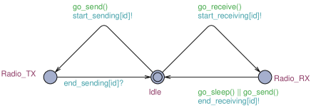
Figure 8: Automaton ${\sf Controller}[{\sf id}]$

bool go_send(){return (r>g)
 ?((csn[id]+1)%C==tsn[id] && clk[id]==k0-(r-g))
 :(csn[id]==tsn[id] && clk[id]==g-r);}

bool go_receive(){return
(r>0 && 0!=tsn[id] && csn[id]==C-1 && clk[id]==k0-r)
|| (r==0 && 0!=tsn[id] && csn[id]==0)
|| (0<csn[id] && csn[id]<n && csn[id]-1==tsn[id]);}

bool go_sleep(){return csn[id]==n;}

Figure 9: Predicates used in ${\sf Controller}[{\sf id}]$

All the channels used in the ${\sf Controller}[{\sf id}]$ automaton (${\sf start\_sending}$, ${\sf end\_sending}$, ${\sf start\_receiving}$, ${\sf end\_receiving}$ and ${\sf synchronize}$) are urgent, which means that these signals are sent at the moment when the transitions are enabled.

Synchronizer

Finally, automaton ${\sf Synchronizer}[{\sf id}]$ is shown in Figure 11. The automaton maintains a list of phase differences of all messages received in the current frame, using a local array ${\sf phase\_errors}$. Local variable ${\sf msg\_counter}$ records the number of messages received.

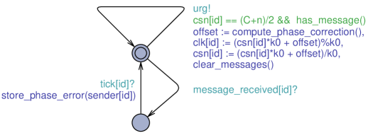
Figure 10: Automaton ${\sf Synchronizer}[{\sf id}]$

        void store_phase_error(int sender)
        {
        phase_errors[msg_counter] =
           (tsn[sender] * k0 + k0 - g)
                - (csn[id] * k0 + clk[id]);
        msg_counter++
        }

Figure 11: Function used in ${\sf Synchronizer}[{\sf id}]$

Whenever the receiver gets a message from a neighboring node (${\sf message\_received}[{\sf id}]$), the synchronizer computes and stores the phase difference using the function ${\sf store\_phase\_error}$ at the next clock tick. Here the phase difference is defined as the expected time at which the message transmission ends (tsn[sender] * k0 + k0 - g) minus the actual time at which the message transmission ends (csn[id] * k0 + clk[id]), counting from the start of the frame. The complete definition is listed in Figure 11. Recall that in our model we abstract from transmission delays.

As explained in Section 2.1, the synchronizer computes the value of the phase correction (offset) and adjusts the clock during the sleeping period of a frame. Hence, in order to decide in which slot we may perform the synchronization, we need to know the maximal phase difference between two nodes. In our model, we assume no joining of networks. When a node receives a message from another node, the phase difference computed using this message will not exceed the length of an active period. Otherwise one of these two nodes will be in sleeping period while the other is sending, hence no message can be received at all. In practice, the number of sleeping slots is much larger than the number of active slots. Therefore it is safe to perform the adjustment in the middle of sleeping period because the desired property described above holds. When the value of gain is smaller than $1$ the maximal phase difference will be even smaller.

The function of ${\sf compute\_phase\_correction}$ implements exactly the algorithm listed in Section 2.1.

4 Analysis Results

In this section, we present some verification results that we obtained for simple instances of the model that we described in Section 3. We checked the following invariant properties using the Uppaal model checker:

INV1 : A[] forall (i: Nodes) forall (j : Nodes)
   SENDER(i).Sending && neighbor(i,j)imply RECEIVER(j).Receiving

INV2 : A[] forall (i:Nodes) forall (j:Nodes) forall (k:Nodes)
   SENDER(i).Sending && neighbor(i,k) && SENDER(j).Sending && neighbor(j,k)
                   imply i == j

INV3 : A[] not deadlock

The first property states that always when some node is sending, all its neighbors are listening. The second property states that never two different neighbors of a given node are sending simultaneously. The third property states that the model contains no deadlock, in the sense that in each reachable state at least one component can make progress. The three invariants are basic sanity properties of the gMAC protocol, at least in a setting with a static topology and no transmission failures.

We used Uppaal on a Sun Fire X4440 machine (with 4 Opteron 8356 2.3 Ghz quad-core processors and 128 Gb DDR2-667 memory) to verify instances of our model with different number of nodes, different network topologies and different parameter values. Table 2 lists some of our verification results, including the resources Uppaal needed to verify if the network is synchronized or not. In all experiments, ${\sf C}=10$ and ${\sf k_{0}}=29$.

${\sf N}/{\sf n}$	Topology	${\sf g}$	${\sf r}$	$\frac{{\sf min}}{{\sf max}}$	CPU Time	Peak Memory Usage	Sync
$3/3$	clique	$2$	$0$	$1$	$1.944$ s	$24,180$ KB	YES
$3/3$	clique	$2$	$0$	$\frac{100,000}{100,001}$	$492.533$ s	$158,064$ KB	NO
$3/3$	clique	$2$	$1$	$1$	$1.976$ s	$68.144$ KB	YES
$3/3$	clique	$2$	$0$	$\frac{100,000}{100,001}$	$116.68$ s	$68,144$ KB	NO
$3/3$	line	$2$	$0$	$1$	$1.068$ s	$68,144$ KB	YES
$3/3$	line	$2$	$0$	$\frac{100,000}{100,000}$	$441.308$ s	$68,144$ KB	NO
$3/3$	line	$2$	$1$	$1$	$1.041$ s	$68,144$ KB	YES
$3/3$	line	$2$	$1$	$\frac{100,000}{100,000}$	$99.274$ s	$68,144$ KB	NO
$3/3$	clique	$3$	$0$	$1$	$1.851$ s	$28,040$ KB	YES
$3/3$	clique	$3$	$0$	$\frac{100,000}{100,001}$	$575.085$ s	$272,312$ KB	NO
$3/3$	clique	$4$	$0$	$\frac{350}{351}$	$115.166$ s	$516,636$ KB	NO
$3/3$	clique	$4$	$0$	$\frac{351}{352}$	$147.864$ s	$630,044$ KB	YES
$3/3$	clique	$3$	$2$	$1$	$1.827$ s	$24,184$ KB	YES
$3/3$	clique	$3$	$2$	$\frac{100,000}{100,001}$	$109.633$ s	$26,056$ KB	NO
$3/3$	clique	$4$	$2$	$\frac{100,000}{100,001}$	$533.345$ s	$350,504$ KB	NO
$3/3$	clique	$5$	$2$	$\frac{587}{588}$	$72.473$ s	$332,552$ KB	NO
$3/3$	clique	$5$	$2$	$\frac{588}{589}$	$99.101$ s	$407,884$ KB	YES
$3/3$	clique	$3$	$5$	$1$	$0.076$ s	$21,884$ KB	NO
$3/3$	line	$3$	$0$	$1$	$1.05$ s	$23,348$ KB	YES
$3/3$	line	$3$	$0$	$\frac{451}{452}$	$29.545$ s	$148,012$ KB	NO
$3/3$	line	$3$	$0$	$\frac{452}{453}$	$35.257$ s	$148,012$ KB	YES
$3/3$	line	$3$	$2$	$1$	$1.052$ s	$22,916$ KB	YES
$3/3$	line	$3$	$2$	$\frac{100,000}{100,001}$	$82.383$ s	$78,360$ KB	NO
$3/3$	line	$4$	$2$	$\frac{100,000}{100,001}$	$414.201$ s	$53,752$ KB	NO
$3/3$	line	$5$	$2$	$\frac{453}{454}$	$33.16$ s	$147,796$ KB	NO
$3/3$	line	$5$	$2$	$\frac{454}{455}$	$38.811$ s	$162,184$ KB	YES
$3/3$	line	$3$	$5$	$1$	$0.048$ s	$78,360$ KB	NO
$4/4$	clique	$3$	$0$	$1$	$231.297$ s	$1,437,643$ KB	YES
$4/4$	clique	$3$	$0$	$\frac{450}{451}$	Memory Exhausted
$4/4$	clique	$3$	$2$	$1$	$229.469$ s	$1,438,368$ KB	YES
$4/4$	clique	$3$	$2$	$\frac{100,000}{100,001}$	$14,604.531$ s	$2,317,040$ KB	NO
$4/3$	line	$3$	$0$	$1$	$4.749s$ s	$94,748$ KB	YES
$4/3$	line	$3$	$0$	$\frac{450}{451}$	Memory Exhausted
$4/3$	line	$3$	$2$	$1$	$4.738$ s	$94,748$ KB	YES
$4/3$	line	$3$	$2$	$\frac{100,000}{100,001}$	$1,923.655$ s	$1,264,844$ KB	YES
$5/5$	clique	$3$	$0$	$1$	Memory Exhausted
$5/5$	clique	$3$	$2$	$1$	Memory Exhausted
$5/3$	line	$3$	$0$	$1$	$46.54$ s	$249,976$ KB	YES
$5/3$	line	$3$	$2$	$1$	$46.489$ s	$250,880$ KB	YES
$6/3$	line	$3$	$0$	$1$	$508.19$ s	$2,316,416$ KB	YES
$6/3$	line	$3$	$2$	$1$	$502.871$ s	$2,317,040$ KB	YES
$7/3$	line	$3$	$0$	$1$	Memory Exhausted
$7/3$	line	$3$	$2$	$1$	Memory Exhausted

Table 2: Model checking experiments

Clearly, the values of network parameters, in particular clock parameters ${\sf min}$ and ${\sf max}$, affect the result of the verification. Table 2 shows several instances where the protocol is correct for perfect clocks (${\sf min}={\sf max}$) but fails when we decrease the ratio $\frac{{\sf min}}{{\sf max}}$. It is easy to see that the protocol will always fail when ${\sf r}\geq{\sf g}$. Consider any node $i$ that is not the last one to transmit within a frame. Right after its sending slot, node $i$ needs ${\sf r}$ ticks to get its radio into receiving mode. This means that — even with perfect clocks — after ${\sf g}$ ticks another node already has started sending even though the radio of node $i$ is not yet receiving. Even when ${\sf r}<{\sf g}$, the radio switching time has a clear impact on correctness: the larger the radio switching time is, the larger the guard time has to be in order to ensure correctness. Using Uppaal, we can fully analyze line topologies with at most seven nodes if all clocks are perfect. For larger networks Uppaal runs out of memory. A full parametric analysis of this protocol will be challenging, also due to the impact of the network topology and the selected slot allocation. Using Uppaal, we discovered that for certain topologies and slot allocations the Median algorithm may always violate the above correctness assertions, irrespective of the choice of the guard time. For example, in a $4$ node-network with clique topology and ${\sf min}$ and ${\sf max}$ of $100.000$ and $100.001$, respectively, if the median of the clock drifts of a node becomes $-1$, the median algorithm divides it by $2$ and generates $0$ for clock correction value and indeed no synchronization happens. If this scenario repeats in three consecutive time frames for the same node, that node runs ${\sf g}=3$ clock cycles behind and gets out of sync.

Another example in which the algorithm may fail is displayed in Figure 12. This network has 4 nodes, connected by a line topology, that send in slots 1, 2, 3, 1, respectively.

Figure 12: A problematic network configuration

Since all nodes have at most two neighbors, the Median algorithm prescribes that nodes will correct their clocks based on the first phase error that they see in each frame. For the specific topology and slot allocation of Figure 12, this means that node 0 adjusts its clock based on phase errors of messages it gets from node 1, node 1 adjusts its clock based on messages from node 0, node 2 adjusts its clock based on messages from node 3, and node 3 adjusts its clock based on messages from node 2. Hence, for the purpose of clock synchronization, we have two disconnected networks! Thus, if the clock rates of nodes 0 and 1 are lower than the clock rates of nodes 2 and 3 by just an arbitrary small margin, then two subnetworks will eventually get out of sync. These observations are consistent with results that we obtained using Uppaal. If, for instance, we set ${\sf min}[{\sf id}]=99$ and ${\sf max}[{\sf id}]=100$, for all nodes ${\sf id}$ then neither INV1 nor INV2 holds. In practice, it is unlikely that the above scenario will occur due to the fact that in the implementation slot allocation is random and dynamic. Due to regular changes of the slot allocation, with high probability node 1 and node 2 will now and then adjusts their clocks based on messages they receive from each other.

However, variations of the above scenario may occur in practice, even in a setting with dynamic slot allocation. In fact, the above synchronization problem is also not restricted to line topologies. We call a subset $C$ of nodes in a network a community if each node in $C$ has more neighbors within $C$ than outside $C$ [14]. For any network in which two disjoint communities can be identified, the Median algorithm allows for scenarios in which these two parts become unsynchronized. Due to the median voting mechanism, the phase errors of nodes outside a community will not affect the nodes within this community, independent of the slot allocation. Therefore, if nodes in one community $A$ run slow and nodes in another community $B$ run fast then the network will become unsynchronized eventually, even in a setting with infinitesimal clock drifts. Figure 13 gives an example of a network with two communities.

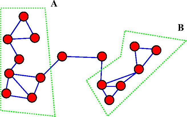
Figure 13: Another problematic network configuration with two communities

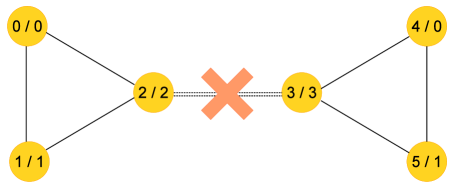
Figure 14: A network with two communities that we analyzed using Uppaal

Using Uppaal, we succeeded to analyze instances of the simple network with two communities displayed in Figure 14. The numbers on the vertices are the node identifiers and the transmission slot numbers, respectively. Table 3 summarizes the results of our model checking experiments.

${\sf g}$	${\sf r}$	Fast Clock	Slow Clock	CPU Time	Peak Memory Usage
		Cycle Length	Cycle Length
$2$	$0$	$1$	$1$	Memory Exhausted
$2$	$0$	$99$	$100$	$457.917$ s	$2,404,956$ KB
$2$	$1$	$99$	$100$	$445.148$ s	$2,418,032$ KB
$3$	$0$	$99$	$100$	$416.796$ s	$2,302,548$ KB
$3$	$2$	$1$	$1$	Memory Exhausted
$3$	$2$	$99$	$100$	$22.105$ s	$83,476$ KB
$3$	$2$	$451$	$452$	$798.121$ s	$3,859,104$ KB
$3$	$2$	$452$	$453$	Memory Exhausted
$4$	$0$	$99$	$100$	$424.935$ s	$2,323,004$ KB
$4$	$1$	$99$	$100$	$464.503$ s	$2,462,176$ KB
$4$	$2$	$99$	$100$	$420.742$ s	$2,323,952$ KB

Table 3: Model checking experiments of a network with two communities

We still need to explore how realistic our counterexamples are. We believe that network topologies with multiple communities occur in many WSN applications. Nevertheless, in practice the gMAC protocol appears to perform quite well for static networks. It might be that problems do not occur so often in practice due to the probabilistic distributions of clock drift and jitter.

5 Conclusions

We presented a detailled Uppaal model of relevant parts of the clock synchronization algorithm that is currently being used in a wireless sensor network that has been developed by Chess [16, 21]. The final model that we presented here may look simple, but the road towards this model was long and we passed through numerous intermediate versions on the way. Using Uppaal, we established that in certain cases a static, fully synchronized network may eventually become unsynchronized if the current Median algorithm is used, even in a setting with infinitesimal clock drifts.

In [10], we proposed a slight variation of the gMAC algorithm that does not have the correctness problems of the Median algorithm. However, our algorithm still has to be tested in practice. Assegei [2] proposed and simulated three alternative algorithms, to be used instead of the Median algorithm, in order to achieve decentralized, stable and energy-efficient synchronization of the Chess gMAC protocol. It should be easy to construct Uppaal models for Assegei’s algorithms: basically, we only have to modify the definition of the compute_phase_correction function. Recently, Pussente & Barbosa [15], also proposed a very interesting new clock synchronization algorithm — in a somewhat different setting — that achieves an $O(1)$ worst-case skew between the logical clocks of neighbors. Much additional research is required to analyze correctness and performance of these algorithms in the realistic settings of Chess with large networks, message loss, and network topologies that change dynamically. Starting from our current Uppaal model, it should be relatively easy to construct models for the alternative synchronization algorithms in order to explore their properties.

Analysis of clock synchronization algorithms for wireless sensor networks is an extremely challenging area for quantitative formal methods. One challenge is to come up with the right abstractions that will allow us to verify larger instances of our model. Another challenge is to make more detailled (probabilistic) models of radio communication and to apply probabilistic model checkers and specification tools such as PRISM [11] and CaVi [7].

Several other recent papers report on the application of Uppaal  for the analysis of protocols for wireless sensor networks, see e.g. [8, 7, 19, 10]. In [22], Uppaal is also used to automatically test the power consumption of wireless sensor networks. Our paper confirms the conclusions of [8, 19]: despite the small number of nodes that can be analyzed, model checking provides valuable insight in the behavior of protocols for wireless sensor networks, insight that is complementary to what can be learned through the application of simulation and testing.

Acknowledgement

We are most grateful to Frits van der Wateren for his patient explanations of the subtleties of the gMAC protocol. We thank Hernán Baró Graf for spotting a mistake in an earlier version of our model, and Mark Timmer for pointing us to the literature on communities in networks. Finally, we thank the anonymous reviewers for their comments.

References

- [1]
- [2] F.A. Assegei (2008): Decentralized frame synchronization of a TDMA-based wireless sensor network. Master’s thesis, Eindhoven University of Technology, Department of Electrical Engineering.
- [3] G. Behrmann, A. David, K. G. Larsen, J. Håkansson, P. Pettersson, W. Yi & M. Hendriks (2006): Uppaal 4.0. In: Third International Conference on the Quantitative Evaluation of SysTems (QEST 2006), 11-14 September 2006, Riverside, CA, USA. IEEE Computer Society, pp. 125–126.
- [4] G. Behrmann, A. David & K.G. Larsen (2004): A Tutorial on Uppaal. In: M. Bernardo & F. Corradini, editors: Formal Methods for the Design of Real-Time Systems, International School on Formal Methods for the Design of Computer, Communication and Software Systems, SFM-RT 2004, Bertinoro, Italy, September 13-18, 2004, Revised Lectures, Lecture Notes in Computer Science 3185. Springer, pp. 200–236.
- [5] J. Bengtsson, W.O.D. Griffioen, K.J. Kristoffersen, K.G. Larsen, F. Larsson, P. Pettersson & Wang Yi (1996): Verification of an Audio Protocol with Bus Collision Using UPPAAL. In: R. Alur & T.A. Henzinger, editors: Proceedings of the 8th International Conference on Computer Aided Verification, New Brunswick, NJ, USA, Lecture Notes in Computer Science 1102. Springer-Verlag, pp. 244–256.
- [6] R. Fan & N.A. Lynch (2006): Gradient Clock Synchronization. Distributed Computing 18(4), pp. 255–266.
- [7] A. Fehnker, M. Fruth & A. McIver (2009): Graphical Modelling for Simulation and Formal Analysis of Wireless Network Protocols. In: M. Butler, C.B. Jones, A. Romanovsky & E. Troubitsyna, editors: Methods, Models and Tools for Fault Tolerance, Lecture Notes in Computer Science 5454. Springer, pp. 1–24.
- [8] A. Fehnker, L. van Hoesel & A. Mader (2007): Modelling and Verification of the LMAC Protocol for Wireless Sensor Networks. In: J. Davies & J. Gibbons, editors: Integrated Formal Methods, 6th International Conference, IFM 2007, Oxford, UK, July 2-5, 2007, Proceedings, Lecture Notes in Computer Science 4591. Springer, pp. 253–272. Available at http://dx.doi.org/10.1007/978-3-540-73210-5_14.
- [9] K. Havelund, A. Skou, K.G. Larsen & K. Lund (1997): Formal modeling and analysis of an audio/video protocol: an industrial case study using UPPAAL. In: Proceedings of the 18th IEEE Real-Time Systems Symposium (RTSS ’97), December 3-5, 1997, San Francisco, CA, USA. IEEE Computer Society, pp. 2–13.
- [10] F. Heidarian, J. Schmaltz & F.W. Vaandrager (2009): Analysis of a Clock Synchronization Protocol for Wireless Sensor Networks. In: A. Cavalcanti & D. Dams, editors: Proceedings 16th International Symposium of Formal Methods (FM2009), Eindhoven, the Netherlands, November 2-6, 2009, Lecture Notes in Computer Science 5850. Springer, pp. 516–531.
- [11] M.Z. Kwiatkowska, G. Norman & D. Parker (2004): PRISM 2.0: A Tool for Probabilistic Model Checking. In: Proceedings of the 1st International Conference on Quantitative Evaluation of Systems (QEST04). IEEE Computer Society, pp. 322–323.
- [12] C. Lenzen, T. Locher & R. Wattenhofer (2008): Clock Synchronization with Bounded Global and Local Skew. In: 49th Annual IEEE Symposium on Foundations of Computer Science, FOCS 2008, October 25-28, 2008, Philadelphia, PA, USA. IEEE Computer Society, pp. 509–518. Available at http://dx.doi.org/10.1109/FOCS.2008.10.
- [13] L. Meier & L. Thiele (2005): Gradient Clock Synchronization in Sensor Networks. Technical Report 219, Computer Engineering and Networks Laboratory, ETH Zurich.
- [14] M.E.J. Newman (2004): Detecting community structure in networks. The European Physical Journal B 38, pp. 321–330.
- [15] R.M. Pussente & V.C. Barbosa (2009): An algorithm for clock synchronization with the gradient property in sensor networks. Journal of Parallel and Distributed Computing 69(3), pp. 261 – 265. Available at http://www.sciencedirect.com/science/article/B6WKJ-4TYJTY5-1/%2/38716d7d9f37c51edb8ba05e508fa2ce.
- [16] QUASIMODO (2009). Preliminary description of case studies. Available at http://www.quasimodo.aau.dk/safe_html/internal/Deliverables/F%inal/Deliverable-5.2.pdf. Deliverable 5.2 from the FP7 ICT STREP project 214755 (QUASIMODO).
- [17] B. Sundararaman, U. Buy & A. D. Kshemkalyani (2005): Clock synchronization for wireless sensor networks: a survey. Ad Hoc Networks 3(3), pp. 281 – 323. Available at http://www.sciencedirect.com/science/article/B7576-4FDMVS4-1/%2/63ed40b032c6bf3ad5fca7fdcbe9e35a.
- [18] R. Tjoa, K.L. Chee, P.K. Sivaprasad, S.V. Rao & J.G Lim (2004): Clock drift reduction for relative time slot TDMA-based sensor networks. In: Proceedings of the IEEE International Symposium on Personal, Indoor and Mobile Radio Communications (PIMRC2004). pp. 1042–1047.
- [19] S. Tschirner, L. Xuedong & W. Yi (2008): Model-based validation of QoS properties of biomedical sensor networks. In: L. de Alfaro & J. Palsberg, editors: Proceedings of the 8th ACM & IEEE International conference on Embedded software, EMSOFT 2008, Atlanta, GA, USA, October 19-24, 2008. ACM, pp. 69–78.
- [20] F.W. Vaandrager & A.L. de Groot (2006): Analysis of a Biphase Mark Protocol with Uppaal and PVS. Formal Aspects of Computing Journal 18(4), pp. 433–458. Available at http://www.ita.cs.ru.nl/publications/papers/fvaan/BMP.html.
- [21] F. van der Wateren (2009). Personal communication.
- [22] M. Woehrle, K. Lampka & L. Thiele (2009): Exploiting Timed Automata for Conformance Testing of Power Measurements. In: J. Ouaknine & F. W. Vaandrager, editors: Formal Modeling and Analysis of Timed Systems, 7th International Conference, FORMATS 2009, Budapest, Hungary, September 14-16, 2009. Proceedings, Lecture Notes in Computer Science 5813. Springer, pp. 275–290. Available at http://dx.doi.org/10.1007/978-3-642-04368-0_21.