A Model Analysis of Triaxial Deformation Dynamics in Oblate-Prolate Shape Coexistence Phenomena

Abstract

From a viewpoint of oblate-prolate symmetry and its breaking, we adopt the quadrupole collective Hamiltonian to study dynamics of triaxial deformation in shape coexistence phenomena. It accommodates the axially symmetric rotor model, the $\gamma$-unstable model, the rigid triaxial rotor model and an ideal situation for the oblate-prolate shape coexistence as particular cases. Numerical solutions of this model yield a number of interesting suggestions. (1) The relative energy of the excited $0^{+}$ state can be a signature of the potential shape along the $\gamma$ direction. (2) Specific $E2$ transition probabilities are sensitive to the breaking of the oblate-prolate symmetry. (3) Nuclear rotation may induce the localization of collective wave functions in the $(\beta,\gamma)$ deformation space.

1 Introduction

In recent years, experimental data suggesting coexistence of the ground-state rotational band with the oblate shape and the excited band with the prolate shape have been obtained in proton-rich unstable nuclei. [1, 2, 3] Together with a variety of shape coexistence phenomena observed in various regions of nuclear chart, [4, 5, 6, 7] some of which involve the spherical shape also, these discoveries stimulate development of nuclear structure theory capable of describing this new class of phenomena. [8, 9, 10, 11, 12, 13] Recently, Hinohara et al. [14, 15] carried out detailed microscopic calculations for the oblate-prolate shape mixing by means of the adiabatic self-consistent collective coordinate (ASCC) method.[8] They suggest that the excitation spectrum of ⁶⁸Se may be regarded as a case corresponding to an intermediate situation between the well-developed oblate-prolate shape coexistence limit, where the shapes of the two coexisting rotational bands are well localized in the $(\beta,\gamma)$ deformation space, and the $\gamma$-unstable limit, where a large-amplitude shape fluctuation takes place in the $\gamma$ degree of freedom. Here, $\beta$ and $\gamma$ are well-known dynamical variables denoting the magnitude of the quadrupole deformation and the degree of axial symmetry breaking, respectively. These calculations indicate the importance of the coupled motion of the large-amplitude shape fluctuation in the $\gamma$ degree of freedom and the three-dimensional rotation associated with the triaxial shape.

In order to discuss the oblate-prolate shape coexistence phenomena in a wider perspective including their relations to other classes of low-energy spectra of nuclei, we introduce in this paper a simple phenomenological model capable of describing the coupled motion of the large-amplitude $\gamma$-vibrational motions and the three-dimensional rotational motions. We call it (1+3)D model in order to explicitly indicate the numbers of vibrational ($\gamma$) and rotational (three Euler angles) degrees of freedom. This model is able to describe several interesting limits in a unified perspective. It includes the axially symmetric rotor model, the $\gamma$-unstable model, [16] the triaxial rigid rotor model [17] and an ideal situation of the oblate-prolate shape coexistence. It also enables us to describe intermediate situations between these different limits by varying a few parameters. This investigation will provide a new insight concerning connections between microscopic descriptions of oblate-prolate shape mixing and various macroscopic pictures on low-energy spectra in terms of phenomenological models. It is intended to be complementary to the microscopic approach we are developing on the basis of the ASCC method.

The (1+3)D model is introduced on the basis of the well-known five-dimensional (5D) quadrupole collective Hamiltonian [18] by fixing the axial deformation parameter $\beta$. Simple functional forms are assumed for the collective potential and the collective mass (inertial function) with respect to the triaxial deformation $\gamma$. We analyze properties of excitation spectra, quadrupole moments and transition probabilities from a viewpoint of oblate-prolate symmetry and its breaking varying a few parameters characterizing the collective potential and the collective mass. Specifically, we investigate the sensitivity of these properties to 1) the barrier-height between the oblate and prolate local minima in the collective potential, 2) the asymmetry parameter that controls the degree of oblate-prolate symmetry breaking in the collective potential, and 3) the mass-asymmetry parameter introducing the oblate-prolate asymmetry in the vibrational and rotational collective mass functions. Dynamical mechanism determining localization and delocalization of collective wave functions in the deformation space is investigated. We find a number of interesting features which have received little attention until now: 1) the unique behavior of the excited $0^{+}$ state as a function of the barrier-height parameter, 2) specific $E2$ transition probabilities sensitive to the degree of oblate-prolate symmetry breaking, 3) the rotation-assisted localization of collective wave functions in the deformation space. We also examine the validity of the (1+3)D model by taking into account the $\beta$ degree of freedom, i.e., by solving the collective Schrödinger equation for a 5D quadrupole collective Hamiltonian that simulates the situation under consideration.

In the present paper, therefore, we intend to clarify the role of the $\beta$-$\gamma$ dependence of the collective mass. Since the original papers by Bohr and Mottelson, [19, 20] the collective Schrödinger equation with the 5D quadrupole collective Hamiltonian[18] has been widely used as the basic framework to investigate low-frequency quadrupole modes of excitation in nuclei. The collective potential and the collective masses appearing in the Hamiltonian have been introduced either phenomenologically [21, 22, 23, 24] or through microscopic calculations. [25, 26, 27, 28, 29, 31, 32, 33, 34, 35] In recent years, powerful algebraic methods of solving the collective Schrödinger equation have been developed [36, 37] and analytical solutions have been found [38, 39, 40, 41, 42] for some special forms of the collective potential (see the recent review [43] for an extensive list of references). However, all collective masses are assumed to be equal and a constant in these papers[38, 39, 40, 41, 42]. It should be emphasized that this approximation is justified only for harmonic vibrations about the spherical shape. The collective masses express inertia of vibrational and rotational motions, so that they play crucial roles in determining the collective dynamics. In general, they are coordinate-dependent, i.e., functions of $\beta$ and $\gamma$. In fact, various microscopic calculations for the collective masses indicate their significant variations as functions of $\beta$ and $\gamma$. [28, 29, 31, 32, 33, 34, 35, 44, 45, 46, 47, 48] In phenomenological analysis of experimental data, for instance, Jolos and Brentano [49] have shown that it is necessary to use different collective masses for the rotational and $\beta$- and $\gamma$-vibrational modes in order to describe interband $E2$ transitions in prolately deformed nuclei.

This paper is organized as follows. After recapitulating the 5D quadrupole collective Hamiltonian and the collective Schrödinger equation in §2, we introduce in §3 the (1+3)D model of triaxial deformation dynamics. In §4, using the (1+3)D model, we first discuss properties of excitation spectra for the collective potentials possessing oblate-prolate symmetry. We then investigate how they change when this symmetry is broken in the collective potential and/or in the collective mass. In §5 we examine the validity of the (1+3)D model by introducing $\beta$-$\gamma$ coupling effects on the basis of the 5D quadrupole collective Hamiltonian. Concluding remarks are given in §6.

2 Five-dimensional quadrupole collective Hamiltonian

We start with the 5D quadrupole collective Hamiltonian involving five collective coordinates, i.e., two deformation variables ($\beta,\gamma$) and three Euler angles:

$$H =T_{\rm vib}+T_{\rm rot}+V(\beta,\gamma),$$ (1)

$$T_{\rm vib} =\frac{1}{2}D_{\beta\beta}(\beta,\gamma){\dot{\beta}}^{2}+D_{\beta\gamma}(\beta,\gamma){\dot{\beta}}{\dot{\gamma}}+\frac{1}{2}D_{\gamma\gamma}(\beta,\gamma){\dot{\gamma}}^{2},$$ (2)

$$T_{\rm rot} =\sum_{k=1}^{3}\frac{1}{2}\mathcal{J}_{k}(\beta,\gamma)\omega_{k}^{2}.$$ (3)

Here, the collective potential $V(\beta,\gamma)$ is a function of two deformation coordinates, $\beta$ and $\gamma$, which represent the magnitudes of quadrupole deformation and triaxiality, respectively. It must be a scalar under rotation, so that it can be written as a function of $\beta^{2}$ and $\beta^{3}\cos 3\gamma$[18]. As is well known, one can restrict the range of $\gamma$ to be $0^{\circ}\leq\gamma\leq 60^{\circ}$ by virtue of the transformation properties between different choices of the principal axes. The first term $T_{\rm vib}$ in Eq. (1) represents the kinetic energies of shape vibrations; it is a function of $\beta$ and $\gamma$ as well as their time derivatives $\dot{\beta}$ and $\dot{\gamma}$. The second term $T_{\rm rot}$ represents the rotational energy written in terms of three angular velocities $\omega_{k}$ which are related to the time derivatives of the Euler angles. The three moments of inertia can be written as

$$\mathcal{J}_{k}(\beta,\gamma)=4\beta^{2}D_{k}(\beta,\gamma)\sin^{2}\gamma_{k},$$ (4)

with respect to the principal axes ($k=1-3$), where $\gamma_{k}=\gamma-(2\pi k)/3$. In this paper, we adopt Bohr-Mottelson’s notation [18] for the six collective mass functions, $D_{\beta\beta},D_{\beta\gamma},D_{\gamma\gamma},D_{1},D_{2}$ and $D_{3}$. They must fulfill the following conditions,

$$D_{1}(\beta,\gamma=0^{\circ}) =D_{2}(\beta,\gamma=0^{\circ}),$$ (5)

$$D_{3}(\beta,\gamma=0^{\circ}) =D_{\gamma\gamma}(\beta,\gamma=0^{\circ})\beta^{-2},$$ (6)

$$D_{1}(\beta,\gamma=60^{\circ}) =D_{3}(\beta,\gamma=60^{\circ}),$$ (7)

$$D_{2}(\beta,\gamma=60^{\circ}) =D_{\gamma\gamma}(\beta,\gamma=60^{\circ})\beta^{-2},$$ (8)

in the prolate ($\gamma=0^{\circ}$) and the oblate ($\gamma=60^{\circ}$) axially symmetric limits.[27]

The classical collective Hamiltonian (1) is quantized according to the Pauli prescription. Then, the explicit expressions for the vibrational and rotational kinetic energies are given by [26]

$$\hat{T}_{\rm vib}=\frac{-\hbar^{2}}{2\sqrt{WR}}\left\{\frac{1}{\beta^{4}}\left[\partial_{\beta}\left(\beta^{2}\sqrt{\frac{R}{W}}D_{\gamma\gamma}\partial_{\beta}\right)-\partial_{\beta}\left(\beta^{2}\sqrt{\frac{R}{W}}D_{\beta\gamma}\partial_{\gamma}\right)\right]\right.$$

$$\left.+\frac{1}{\beta^{2}\sin 3\gamma}\left[-\partial_{\gamma}\left(\sqrt{\frac{R}{W}}\sin 3\gamma D_{\beta\gamma}\partial_{\beta}\right)+\partial_{\gamma}\left(\sqrt{\frac{R}{W}}\sin 3\gamma D_{\beta\beta}\partial_{\gamma}\right)\right]\right\}$$ (9)

and

$$\hat{T}_{\rm rot}=\sum_{k=1}^{3}\frac{\hat{I}_{k}^{2}}{2\mathcal{J}_{k}(\beta,\gamma)},$$ (10)

respectively, where $W$ and $R$ are the abbreviations of

$$W(\beta,\gamma) =\beta^{-2}\left[D_{\beta\beta}(\beta,\gamma)D_{\gamma\gamma}(\beta,\gamma)-D_{\beta\gamma}^{2}(\beta,\gamma)\right],$$ (11)

$$R(\beta,\gamma) =D_{1}(\beta,\gamma)D_{2}(\beta,\gamma)D_{3}(\beta,\gamma),$$ (12)

and ${\hat{I}_{k}}$ are the angular momentum operators with respect to the principal-axis frame associated with a rotating deformed nucleus (the body-fixed PA frame).

The collective Schrödinger equation is written as

$$[\hat{T}_{\rm vib}+\hat{T}_{\rm rot}+V(\beta,\gamma)]\Psi_{IM\alpha}(\beta,\gamma,\Omega)=E_{I,\alpha}\Psi_{IM\alpha}(\beta,\gamma,\Omega),$$ (13)

where the collective wave function $\Psi_{IM\alpha}(\beta,\gamma,\Omega)$ is specified by the total angular momentum $I$, its projection $M$ onto the $z$-axis in the laboratory frame and $\alpha$ distinguishing eigenstates possessing the same values of $I$ and $M$. In Eq. (13), $\Omega$ denotes a set of the three Euler angles, which are here dynamical variables describing the directions of the body-fixed PA frame with respect to the laboratory frame. Using the rotational wave functions $\mathcal{D}^{I}_{MK}(\Omega)$, the orthonormalized collective wave functions in the laboratory frame can be written as

$$\Psi_{IM\alpha}(\beta,\gamma,\Omega)=\sum_{K}\Phi_{IK\alpha}(\beta,\gamma)\langle\Omega|IMK\rangle,$$ (14)

where

$$\langle\Omega|IMK\rangle=\sqrt{\frac{2I+1}{16\pi^{2}(1+\delta_{K0})}}\left(\mathcal{D}^{I}_{MK}(\Omega)+(-)^{I}\mathcal{D}^{I}_{M-K}(\Omega)\right).$$ (15)

The functions $\Phi_{IK\alpha}(\beta,\gamma)$ are vibrational wave functions orthonormalized by

$$\int d\tau^{\prime}\sum_{K}\Phi^{\ast}_{IK\alpha}(\beta,\gamma)\Phi_{IK\alpha^{\prime}}(\beta,\gamma)=\delta_{\alpha\alpha^{\prime}}$$ (16)

with the intrinsic volume element

$$d\tau^{\prime}=2\beta^{4}\sqrt{W(\beta,\gamma)R(\beta,\gamma)}\sin{3\gamma}d\beta d\gamma.$$ (17)

In Eqs. (14) and (16), the sum is taken over even values of $K$ from 0 to $I$ for even $I$ (from 2 to $I-1$ for odd $I$). Detailed discussions on the symmetries and boundary conditions in the vibrational wave functions $\Phi_{IK\alpha}(\beta,\gamma)$ are given, e.g., in Ref. 27).

3 Reduction to the (1+3)-dimensional collective Hamiltonian

For the reason mentioned in §1, we are particularly interested in triaxial deformation dynamics. In order to concentrate on the $\gamma$ degree of freedom, we introduce a simple (1+3)D model involving only one vibrational coordinate $\gamma$ and three rotational coordinates. This is done by freezing the $\beta$ degree of freedom in the 5D quadrupole collective Hamiltonian (2.1) as explained below.

The collective potential of this model takes a very simple form:

$$V(\gamma)=V_{0}\sin^{2}3\gamma+V_{1}\cos 3\gamma.$$ (18)

This form is readily obtained by retaining up to the second order with respect to $\beta^{3}\cos 3\gamma$ and fixing $\beta$ at a constant value in an expansion of $V(\beta,\gamma)$ in powers of $\beta^{2}$ and $\beta^{3}\cos 3\gamma$.[50] When $V_{1}=0$, the collective potential is symmetric about $\gamma=30^{\circ}$ with respect to the transformation $\gamma\to 60^{\circ}-\gamma$. For brevity, let us call this symmetry and transformation OP (oblate-prolate) symmetry and OP inversion, respectively. For positive $V_{0}$, two degenerate minima appear at the oblate ($\gamma=60^{\circ}$) and the prolate ($\gamma=0^{\circ}$) shapes, and they are separated by a barrier that takes the maximum at $\gamma=30^{\circ}$. We therefore call $V_{0}$ barrier-height parameter. On the other hand, the maximally triaxial shape at $\gamma=30^{\circ}$ becomes the minimum for negative $V_{0}$, and it becomes deeper as $|V_{0}|$ increases. When $V_{1}\neq 0$, the OP symmetry is broken, and the oblate (prolate) shape becomes the minimum for a combination of positive $V_{0}$ and positive (negative) $V_{1}$. We call $V_{1}$ asymmetry parameter after its controlling the magnitude of the OP symmetry breaking. Thus, by varying the two parameters $V_{0}$ and $V_{1}$, we can see how the excitation spectrum depends on the barrier height and symmetry breaking between the two local minima in the collective potential.

We present in Fig. 1 some examples of the collective potential $V(\gamma)$ that seem to be relevant to a variety of oblate-prolate shape coexistence phenomena. In this figure, we can clearly see how the asymmetry between the oblate and prolate minima grows as a function of $V_{1}$ and how the barrier height measured from the second minimum sensitively depends on the ratio of $V_{1}$ to $V_{0}$.

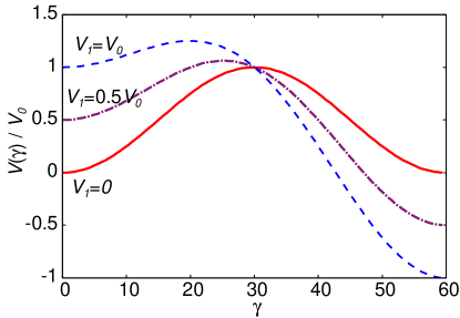
Figure 1: The collective potentials $V(\gamma)$ defined by Eq. (2.4) are plotted for the $V_{0}>0$ case with solid, dash-dotted and dashed lines as functions of $\gamma$ for $V_{1}/V_{0}=0.0,0.5$ and $1.0$, respectively.

The vibrational kinetic energy term reduces, in the (1+3)D model Hamiltonian, to the following form:

$$\hat{T}_{\rm vib}=\frac{-\hbar^{2}}{2\sqrt{D_{\gamma\gamma}(\beta_{0},\gamma)R(\beta_{0},\gamma)}}\frac{1}{\sin 3\gamma}\partial_{\gamma}\left(\sqrt{\frac{R(\beta_{0},\gamma)}{D_{\gamma\gamma}(\beta_{0},\gamma)}}\sin 3\gamma\partial_{\gamma}\right).$$ (19)

We parametrize the collective mass functions as

$$D_{\gamma\gamma}(\gamma) \equiv D_{\gamma\gamma}(\beta_{0},\gamma)=D\beta_{0}^{2}(1+\epsilon\cos 3\gamma),$$ (20)

$$D_{k}(\gamma) \equiv D_{k}(\beta_{0},\gamma)\hskip 5.0pt=D(1+\epsilon\cos\gamma_{k}).$$ (21)

These are the most simple forms involving only one parameter $\epsilon$ that controls the degree of OP symmetry breaking in these four mass functions under the requirement that they should fulfill the conditions (5)–(8). We call $\epsilon$ mass-asymmetry parameter. These functional forms are obtainable also by taking the lowest-order term that brings about the OP symmetry breaking in the expressions of the collective mass functions microscopically derived by Yamada[48] using the SCC method. [51] In this paper, we use $\beta_{0}^{2}=0.1$ and $D=50$ MeV^-1, which roughly simulate the values obtained in the microscopic ASCC calculation[14, 15].

We solve the collective Schrödinger equation (13) replacing $V(\beta,\gamma)$, $\hat{T}_{\rm vib}$ and $\mathcal{J}_{k}(\beta,\gamma)$ in $\hat{T}_{\rm rot}$ by Eqs. (18), (19) and $\mathcal{J}_{k}(\beta_{0},\gamma)$, respectively, with Eqs.  (20) and  (21). Accordingly, the collective wave function is denoted $\Psi_{IM\alpha}(\gamma,\Omega)$. Note that the sign change $V_{1}\to-V_{1}$ corresponds to the OP inversion. One can then easily confirm that the OP inversion is equivalent to the simultaneous sign change of the parameters, $(\epsilon,\pm V_{1})\to(-\epsilon,\mp V_{1})$, in the (1+3)D model Hamiltonian. Therefore, it is enough to study only the case of positive $\epsilon$.

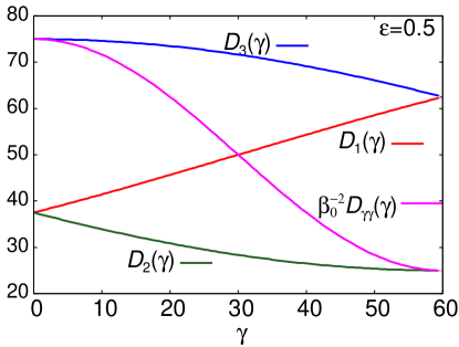
(a) Mass Parameters

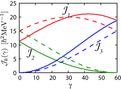
(b) Moments of Inertia

Figure 2: (a) The vibrational and rotational collective mass functions $D_{\gamma\gamma}(\gamma)$ and $D_{k}(\gamma)$, defined by Eqs. (2.2) and (2.3), are plotted as functions of $\gamma$ for the mass-asymmetry parameter $\epsilon=0.5$. (b) Three rotational moments of inertia $\mathcal{J}_{k}(\beta,\gamma)$ with $k=$1, 2 and 3, defined by Eqs. (1.2) and (2.3), are plotted with solid lines as functions of $\gamma$ for the mass-asymmetry parameter $\epsilon=0.5$. The magnitude of the quadrupole deformation $\beta$ is fixed at $\beta^{2}=0.1$. For comparison, the moments of inertia for the $\epsilon=0$ case are also plotted with dashed lines.

Figure 2(a) shows, for an example of $\epsilon=0.5$, how the collective mass functions $D_{\gamma\gamma}$ and $D_{k}$ behave as functions of $\gamma$. Figure 2(b) indicates the degree of oblate-prolate asymmetry in the moments of inertia $\mathcal{J}_{k}(\gamma)$ brought about by the terms involving $\epsilon$. From these figures we can anticipate that, for positive (negative) $\epsilon$ and under the parameterizations of Eqs. (20) and (21), the rotational energy favors the oblate (prolate) shape while the vibrational energy prefers the prolate (oblate) shape.

4 Triaxial deformation dynamics

We have built a new computer code to solve the collective Schrödinger equation (13) for general 5D quadrupole collective Hamiltonian as well as its reduced version for the (1+3)D model. Numerical algorithm similar to that of Kumar and Baranger [27] is adopted in this code, except that we discretize the ($\beta,\gamma$) plane using meshes in the $\beta$ and $\gamma$ directions in place of their triangular mesh. Numerical accuracy and convergence were checked by comparing our numerical results with analytical solutions in the spherical harmonic vibration limit, in the so-called square-well type $\beta$ dependence limit and in the $\gamma$-unstable model. [16] In the following, we discuss how the solutions of the collective Schrödinger equation depend on the barrier-height parameter $V_{0}$, the asymmetry parameter $V_{1}$ and the mass-asymmetry parameter $\epsilon$. We use the adjectives yrast and yrare for the lowest and the second-lowest states for a given angular momentum $I$, respectively, and distinguish the two by suffices as $I_{1}$ and $I_{2}$.

4.1 Excitation spectra in the presence of OP symmetry

Let us first discuss the situation where $V_{1}=0$ and $\epsilon=0$. In this case, both the collective potential and the collective mass functions are symmetric about $\gamma=30^{\circ}$, so that the (1+3)D model Hamiltonian possesses OP symmetry. Furthermore, the collective mass parameter $D$ and $\beta_{0}$ enter the collective Schödinger equation only in the form of the overall factor $(2D\beta_{0}^{2})^{-1}$ in the kinetic energy terms. Hence, only the ratio of the barrier-height parameter $V_{0}$ to this factor is important to determine the collective dynamics. In the particular case of $V_{0}=0$, i.e., $V(\gamma)=0$, which is well known as the Wilets-Jean $\gamma$-unstable model,[16] the excitation spectra are completely scaled by this factor.

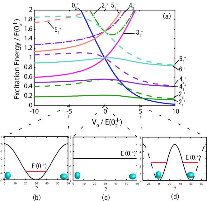
Figure 3: In the upper panel (a), dependence of excitation spectrum on the parameter $V_{0}$ is displayed. Excitation energies as well as $V_{0}$ values are normalized by the excitation energy $E(0_{2}^{+})$ of the second (the first excited) $0^{+}$ state for $V(\gamma)=0$. In the lower panels (b), (c) and (d), the potentials $V(\gamma)$ and the ground $0^{+}$ state energies $E(0_{1}^{+})$ are illustrated for three different values of $V_{0}/E(0_{2}^{+})=-5.0,0.0$ and 5.0, respectively. Note that $E(0_{1}^{+})=0$ for $V_{0}=0$. Because the collective potential $V(\gamma)$ is a periodic function of $60^{\circ}$ in $\gamma$, only the region $0^{\circ}\leq\gamma\leq 60^{\circ}$ is drawn with a solid line in (d).

In Fig. 3, we show the excitation spectra for the case of $V_{1}=0$ and $\epsilon=0$ as functions of $V_{0}$. Here, the excitation energies are normalized by the excitation energy of the first excited $0^{+}$ state (denoted $0_{2}^{+}$) at $V_{0}=0$, $E(0_{2}^{+})$ (which is 1.8 MeV for $\beta_{0}^{2}=0.1$ and $D=50$ MeV^-1 adopted in the present calculation). Accordingly, this figure is valid for any value of $(2D\beta_{0}^{2})^{-1}$ by virtue of the scaling property mentioned above. In the lower panels of this figure, the collective potentials $V(\gamma)$ and the ground $0^{+}$ state energies $E(0_{1}^{+})$ are illustrated for three typical situations: 1) a triaxially deformed case where a deep minimum appears at the triaxial shape with $\gamma=30^{\circ}$, 2) the $\gamma$-unstable case, where the collective potential is flat with respect to $\gamma$, and 3) an extreme case of shape coexistence where the oblate and prolate minima are exactly degenerate in energy. (Strictly, shape coexistence does not appear in a case where the two minima are exactly degenerate as we shall see in Fig. 9.) Note that the collective potential $V(\gamma)$ is a periodic function of $60^{\circ}$ in $\gamma$. Therefore, it is displayed by the solid line only in the region $0^{\circ}\leq\gamma\leq 60^{\circ}$.

In the positive-$V_{0}$ side of this figure, it is clearly seen that a doublet structure emerges when the barrier-height parameter $V_{0}$ becomes very large. In other words, approximately degenerate pairs of eigenstates appear for every angular momentum when $V_{0}/E(0_{2}^{+})\gg 1$. This is nothing but the doublet pattern known well in the problems of double-well potential. [52] In the present case, this doublet structure is associated with the OP symmetry. Furthermore, one immediately notices a very unique behavior of the $0_{2}^{+}$ state. When the barrier-height parameter $V_{0}$ decreases (from the limiting situation mentioned above), its energy rises more rapidly than those of the yrare $2_{2}^{+}$, $4_{2}^{+}$ and $6_{2}^{+}$ states. Thus, a level crossing of the $0_{2}^{+}$ and $2_{2}^{+}$ states takes place at $V_{0}/E(0_{2}^{+})\simeq 3$. When $V_{0}$ further decreases and approaches zero, the excitation energy of the $0_{2}^{+}$ state approaches those of the $4_{2}^{+}$ and $6_{1}^{+}$ states. In the $\gamma$-unstable limit of $V_{0}=0$, they are degenerate.

In the negative-$V_{0}$ side, the excitation energies of the $3_{1}^{+}$ and $5_{1}^{+}$ states drastically decrease as $V_{0}$ decreases, and the excitation spectrum characteristic to the Davydov-Filippov rigid triaxial rotor model [17] appears when the triaxial minimum becomes very deep, i.e., when $V_{0}/E(0_{2}^{+})\ll-1$.

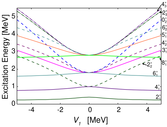
Figure 4: Dependence of excitation spectrum on the asymmetry parameter $V_{1}$ is displayed for the case of $V_{0}=0$.

4.2 Breaking of the OP symmetry in the collective potential

Next, let us investigate effects of the OP-symmetry-breaking term $V_{1}\cos 3\gamma$ in the collective potential $V(\gamma)$. The effects are manifestly seen for the case of $\epsilon=0$ and $V_{0}=0$. We present in Fig. 4 the excitation spectrum for this case as a function of the asymmetry parameter $V_{1}$. For $V_{1}=0$, the spectrum exhibits the degeneracy characteristic to the $\gamma$-unstable model: [16] e.g., the $0_{2}^{+},3_{1}^{+},4_{2}^{+}$ and $6_{1}^{+}$ states are degenerate. With increasing the magnitude of $V_{1}$, such degeneracies are lifted and the yrare $0_{2}^{+},2_{2}^{+},4_{2}^{+}$ and $6_{2}^{+}$ states as well as the odd angular momentum $3_{1}^{+}$ and $5_{1}^{+}$ states rise in energy. As a consequence, the well-known ground-state rotational band spectrum appears for sufficiently large values of $|V_{1}|$. For instance, we can see in Fig. 4 that, as $V_{1}$ increases, the ratio of the yrast $2_{1}^{+}$ and $4_{1}^{+}$ energies, $E(4_{1}^{+})/E(2_{1}^{+})$, increases from 2.5 at $V_{1}=0$, which is the value peculiar to the $\gamma$-unstable model, to be 3.3 for sufficiently large $V_{1}$. This figure beautifully demonstrates the fact that the breaking of spherical symmetry is not sufficient for the appearance of regular rotational spectra even if the magnitude of quadrupole deformation is considerably large: we also need appreciable amount of the OP symmetry breaking. We also note that the spectrum does not depend on the sign of $V_{1}$. This is because, for $\epsilon=0$, both the vibrational and rotational kinetic energy terms in the (1+3)D collective Hamiltonian possess the symmetry under the OP inversion. In short, the inversion $V_{1}\to-V_{1}$ merely interchanges the roles of the oblate and the prolate shapes.

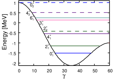
(a) $V_{0}=-2.0$MeV, $V_{1}=1.0$MeV

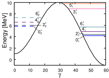
(c) $V_{0}=10.0$MeV, $V_{1}=1.0$MeV

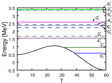
(b) $V_{0}=1.0$MeV, $V_{1}=0.5$MeV

Figure 5: The collective potentials $V(\gamma)$ and eigen-energies are displayed in panels (a), (b) and (c) for $(V_{0},V_{1})=(-2.0,-1.0),(1.0,0.5)$ and (10.0, 1.0) MeV, respectively.

Let us proceed to more general situations where $\epsilon=0$ but both $V_{0}$ and $V_{1}$ are nonzero. Three typical situations are illustrated in Fig. 5. In this figure, the collective potentials and energy spectra are drawn for three different sets of parameters, $(V_{0},V_{1})=(-2,1),(1,0.5)$ and (10, 1) MeV. Panel (a) simulates a situation where the minimum of the collective potential occurs at a triaxial shape but it is rather shallow, so that the potential pocket accommodates only the ground $0^{+}$ state and the first excited $2^{+}$ state. Panel (b) simulates the situation encountered in the microscopic ASCC calculation [14, 15], where two local minima appear both at the oblate and prolate shapes but the barrier between them is so low that strong shape mixing may take place. Panel (c) illustrates an ideal situation for shape coexistence, where the barrier between the oblate and prolate minima is so high that two rotational bands associated with them retain their identities.

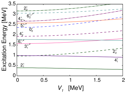
(a) $V_{0}=-2.0$MeV

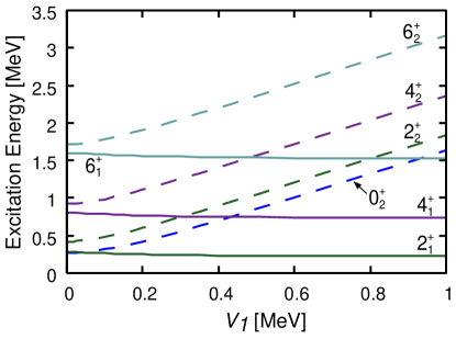
(c) $V_{0}=10.0$MeV

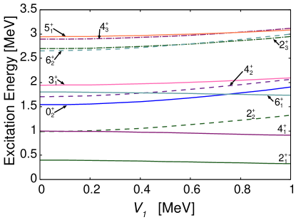
(b) $V_{0}=1.0$MeV

Figure 6: Dependence of excitation spectrum on the asymmetry parameter $V_{1}$ is displayed for $V_{0}=-2.0$ (panel a), 1.0 (panel b) and 10.0 MeV (panel c).

For three typical situations illustrated in Fig. 5, we examine the sensitivity of excitation spectra to the asymmetry parameter $V_{1}$. This is done in Fig. 6, (Panels (a), (b) and (c) display the excitation spectra as functions of $V_{1}$ for $V_{0}=-2,1$ and 10 MeV, respectively.) We see that the dependence on $V_{1}$ is rather weak in the cases (a) and (b). In contrast, the effect of the $V_{1}$ term is extremely strong in the case (c): the approximate doublet structure at $V_{0}=0$ is quickly broken as soon as the $V_{1}$ term is switched on, and the excitation energies of the yrare partners $(0_{2}^{+},2_{2}^{+},4_{2}^{+},6_{2}^{+})$ remarkably increase as $V_{1}$ increases. Quantitatively, the energy splittings between the yrast and yrare states with the same angular momenta are proportional to $V_{1}^{2}$ for $V_{1}\lesssim 0.2$ MeV and then increase almost linearly in the region of $V_{1}\gtrsim 0.2$ MeV. The quadratic dependence on $V_{1}$ in the small-$V_{1}$ region can be understood as the second-order perturbation effects in the double-well problem. In this case, what is important is not the absolute magnitude of $V_{1}$ but its ratio to the energy splitting due to the quantum tunneling through the potential barrier between the two minima. The structure of the collective wave functions is drastically changed by the small perturbation. Indeed, for $V_{1}\gtrsim 0.2$ MeV, they are already well localized in one of the potential pockets, as we shall discuss below in connection with Fig. 9. Once the collective wave functions are well localized, the energy shifts are mainly determined by the diagonal matrix elements of the $V_{1}$ term (with respect to the localized wave functions), leading to the almost linear dependence on $V_{1}$.

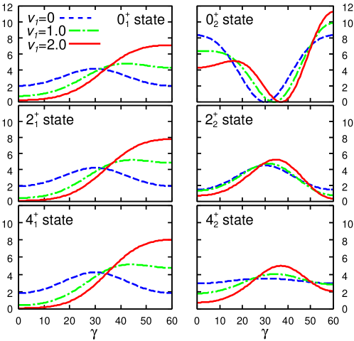
Figure 7: Collective wave functions squared $\sum_{K}|\Phi_{IK\alpha}(\gamma)|^{2}$ of the yrast and the yrare states for the collective potentials $V(\gamma)$ with $V_{1}=0.0,1.0$ and $2.0$ MeV. The barrier-height parameter $V_{0}$ is fixed at $-2.0$ MeV.

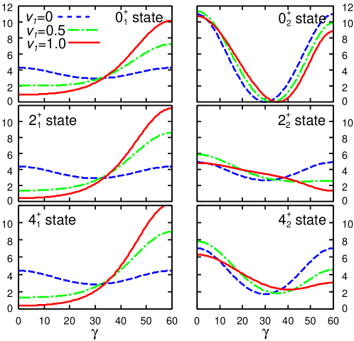
Figure 8: The same as Fig. 7 but for $V_{0}=1.0$ and $V_{1}=$0.0, 0.5 and 1.0 MeV.

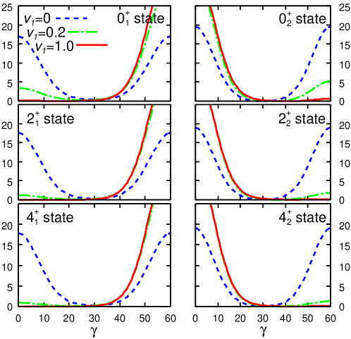
Figure 9: The same as Fig. 7 but for $V_{0}=10.0$ and $V_{1}=$0.0, 0.2 and 1.0 MeV.

The effects of the $V_{1}$ term are seen more clearly in the collective wave functions. Figures 7, 8 and 9 show the collective wave functions squared $\sum_{K}|\Phi_{IK\alpha}(\gamma)|^{2}$ of the yrast and yrare states for $V_{0}=-2,1$ and 10 MeV, which respectively correspond to the potentials in panels (a), (b) and (c) of Fig. 5. In Figs. 7 and 8, one sees that the localization (with respect to the $\gamma$ coordinate) of the collective wave functions of the yrast states grows as $V_{1}$ increases, while that of the yrare states are insensitive to $V_{1}$. This can be easily understood by considering the kinetic-energy effects tend to dominate over the potential-energy effects with increase in the excitation energies. It is interesting to note that in Fig. 8, although the yrast $4_{1}^{+}$ state is situated above the potential barrier, its wave function is well localized around the oblate minimum. Concerning the yrare $4_{2}^{+}$ state, although its wave function has the maximum at the prolate shape due to the orthogonality to the $4_{1}^{+}$ state, it is considerably extended over the entire region of $\gamma$. For the reason mentioned above, the effects of the $V_{1}$ term on localization properties of the yrare states are much weaker than those of the yrast states.

In Fig. 9, we see drastic effects of the $V_{1}$ term. At $V_{1}=0$, the wave functions squared are symmetric about $\gamma=30^{\circ}$. This symmetry is immediately broken after the $V_{1}$ term is switched on: the wave functions of the yrast states rapidly localize around the potential minimum even if the energy difference between the two local minima is very small. In striking contrast to the situation presented in Fig. 8, the wave functions of the yrare states also localize about the second minimum of the potential. We confirmed that $V_{1}$ of 0.2 MeV is sufficient to bring about such strong localization. As pointed out above in connection with the double-well problem, this value of $V_{1}$ is small but comparable to the energy splittings. Thus, one can regard Fig. 9 as a very good example demonstrating that even small symmetry breaking in the collective potential is able to cause a dramatic change in the properties of the collective wave function, provided that the barrier is sufficiently high.

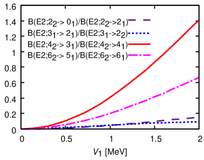
Figure 10: Dependence on the asymmetry parameter $V_{1}$ of selected $E2$ branching ratios that vanish in the oblate-prolate symmetric limit $V_{1}=0$. The barrier-height parameter $V_{0}$ is fixed at $-2.0$ MeV.

In the remaining part of this subsection, we discuss how the $V_{1}$ term affects properties of electric quadrupole ($E2$) transitions and moments. In Fig. 10, the $B(E2)$ ratios that vanish in the $V_{1}=0$ limit are plotted as functions of $V_{1}$ for the $V_{0}=-2.0$ MeV case corresponding to Figs. 5(a), 6(a) and 7. Vanishing of these ratios is well known as one of the signatures of the triaxial shape with $\gamma=30^{\circ}$ in the rigid triaxial rotor model. [17] It should be emphasized, however, that this is in fact a consequence of OP symmetry: these $E2$ transitions vanish due to the exact cancellation between the contribution from the prolate side ($0^{\circ}\leq\gamma<30^{\circ}$) and that from the oblate side ($30^{\circ}<\gamma\leq 60^{\circ}$). Therefore, the localization around $\gamma=30^{\circ}$ is not a necessary condition. In fact, these ratios vanish also in the $\gamma$-unstable model. [16] As anticipated, we see in Fig. 10 that these ratios increase as the collective potential becomes more asymmetric with respect to the oblate and prolate shapes. In particular, the significant rises of the ratios, $B(E2;4_{2}^{+}\rightarrow 3_{1}^{+})/B(E2;4_{2}^{+}\rightarrow 4_{1}^{+})$ and $B(E2;6_{2}^{+}\rightarrow 5_{1}^{+})/B(E2;6_{2}^{+}\rightarrow 6_{1}^{+})$, are remarkable. This may be interpreted as an incipient trend that the sequence of states $(2_{2}^{+},3_{1}^{+},4_{2}^{+},5_{1}^{+}$ and $6_{2}^{+})$ forms a $\gamma$-vibrational bandlike structure about the axially symmetric shape (oblate in the present case) when $V_{1}$ becomes very large.

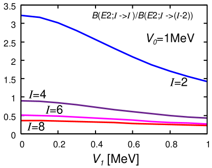
(a) $V_{0}=1.0$MeV

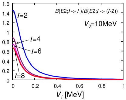
(b) $V_{0}=10.0$MeV

Figure 11: Dependence on the asymmetry parameter $V_{1}$ of the branching ratios $B(E2;I_{\rm yrare}\rightarrow I_{\rm yrast})$/ $B(E2;I_{\rm yrare}\rightarrow(I-2)_{\rm yrare})$. Here, $I_{\rm yrast}$ and $I_{\rm yrare}$ denote the yrast and the yrare states having the same values of angular momenta $I$, while $(I-2)_{\rm yrare}$ the yrare states with angular momentum $I-2$. The left and right panels display the results of calculation for $V_{0}=1.0$ and 10.0 MeV, respectively.

In Fig. 11, the ratios $B(E2;I_{\rm yrare}\rightarrow I_{\rm yrast})$/ $B(E2;I_{\rm yrare}\rightarrow(I-2)_{\rm yrare})$ are plotted as functions of $V_{1}$ for the two cases of $V_{0}=1.0$ and 10.0 MeV. The $V_{0}=1.0$ case corresponds to Figs. 5(b), 6(b) and 8, while the $V_{0}=10.0$ case corresponds to Figs. 5(c), 6(c) and 9. Here, the numerator denotes $B(E2)$ values for $\Delta I=0,~{}E2$ transitions from the yrare to the yrast states with the same angular momenta $I$, while the denominator indicates $\Delta I=-2,~{}E2$ transitions between the yrare states. One immediately notices a sharp contrast between the two cases: when the barrier between the oblate and prolate local minima is very low ($V_{0}=1.0$ MeV), these values are sizable even at $V_{1}=1.0$MeV, although they gradually decrease with increase of $V_{1}$. In contrast, when the barrier is very high ($V_{0}=10.0$ MeV), they quickly decrease once the OP-symmetry-breaking term is turned on. The reason why the interband $E2$ transitions almost vanish is apparent from Fig. 9; the collective wave functions of the yrast and yrare states are well localized around the oblate and prolate shapes, respectively.

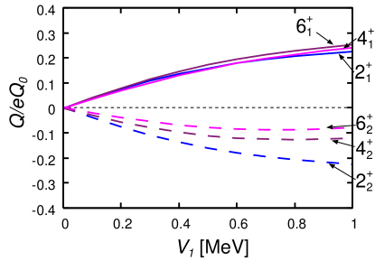
(a) $V_{0}=1.0$MeV

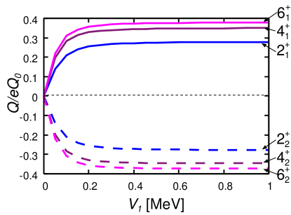
(b) $V_{0}=10.0$MeV

Figure 12: Dependence of the spectroscopic quadrupole moments on the asymmetry parameter $V_{1}$, calculated for $V_{0}=1.0$ MeV (left panel) and $V_{0}=10.0$ MeV (right panel). Their values are plotted in units of the intrinsic quadrupole moment, $eQ_{0}=3e/\sqrt{5\pi}ZR_{0}^{2}\beta_{0}$.

One can further confirm the same point by looking at the spectroscopic quadrupole moments displayed in Fig. 12 in a way parallel to Fig. 11. They vanish in the presence of the OP symmetry due to the exact cancellation between the contributions from the oblate side and from the prolate side. In Fig. 12(a) for the low barrier case ($V_{0}=1.0$ MeV), the quadrupole moments of both the yrast and yrare states first increase after the $V_{1}$ term is switched on, but those for the yrare states eventually saturate. This trend is obvious especially for the $4_{2}^{+}$ and $6_{2}^{+}$ states. These results are easily understandable from the properties of their wave functions displayed in Fig. 8. That is, while the localization in the yrast states develops with $V_{1}$ increasing, the wave functions of the yrare states widely extend over the entire region of $\gamma$, and the effects of the $V_{1}$ term are rather weak. In contrast, Fig. 12(b) for the high barrier case ($V_{0}=10.0$ MeV) demonstrates that both the yrast and yrare states quickly acquire quadrupole moments as soon as the $V_{1}$ term is switched on. This is a direct consequence of the wave function localization displayed in Fig. 9. Note again that the sign change, $V_{1}\leftrightarrow-V_{1}$, corresponds to the OP inversion.

When $V_{0}$ is large and $V_{1}$ is small, just as in the above case, the yrast and the yrare states can be grouped, in a very good approximation, into two rotational bands: one associated with the oblate shape and the other with the prolate shape. This is an ideal situation for the emergence of an oblate-prolate shape coexistence phenomenon. According to the realistic HFB calculations for the collective potential [53], however, it seems hard to obtain such a large value of $V_{0}$. Therefore, for the shape coexistence phenomena we need to take into account dynamical effects going beyond the consideration on the collective potential energies. We shall discuss this point in the succeeding subsection.

4.3 Breaking of OP symmetry in the collective mass

We examine dynamical effects on the localization properties of the collective wave functions. As mentioned in §1, we are particularly interested in understanding the nature of the shape coexistence phenomena observed in nuclei for which approximately degenerate oblate and prolate local minima and a rather low barrier between them are suggested from the microscopic potential energy calculations. [53, 14, 15] In the followings, we therefore concentrate our discussion on the case of the collective potential with a low barrier ($V_{0}=1.0$) and weak OP asymmetry ($V_{1}=0.5$) represented in Fig. 5(b). We shall investigate how the results discussed in the previous subsections for the $\epsilon=0$ case, where the collective mass $D_{\gamma\gamma}(\gamma),D_{k}(\gamma)$ and the rotational moments of inertia $\mathcal{J}_{k}(\gamma)$ are symmetric functions about $\gamma=30^{\circ}$, are modified when the mass-asymmetry parameter $\epsilon$ becomes nonzero.

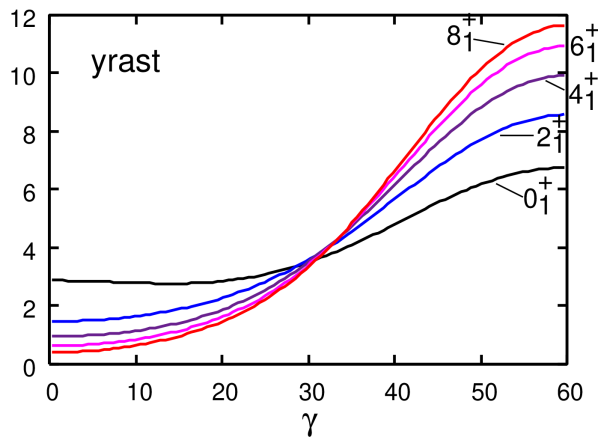
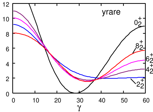
Figure 13: Dependence on angular momentum of the collective wave functions calculated for the mass-asymmetry parameter $\epsilon=0.5$ and the collective potential $V(\gamma)$ with $V_{0}=1.0$ and $V_{1}=0.5$ MeV. The left and the right panels display the results of calculation for the yrast and the yrare states, respectively.

In Fig. 13, the collective wave functions squared $\sum_{K}|\Phi_{IK\alpha}(\gamma)|^{2}$ calculated for $\epsilon=0.5$ are displayed. It is clearly seen that, for the yrast states, the localization around the oblate shape ($\gamma=60^{\circ}$) develops with increase in the angular momentum. The reason is easily understood: for positive $\epsilon$, the rotational moments of inertia perpendicular to the oblate symmetry axis (2nd axis), $\mathcal{J}_{1}(\gamma=60^{\circ})$ and $\mathcal{J}_{3}(\gamma=60^{\circ})$, are larger than those perpendicular to the prolate symmetry axis (3rd axis), $\mathcal{J}_{1}(\gamma=0^{\circ})$ and $\mathcal{J}_{2}(\gamma=0^{\circ})$, as shown in Fig. 2(b). Therefore, the rotational energy for a given angular momentum decreases by increasing the probability of existence around the oblate shape. Since the rotational energy dominates over the vibrational and potential energies, the localization is enhanced for higher angular momentum states. We call this kind of dynamical effect rotation-assisted localization. On the other hand, the wave functions of the yrare states exhibit two-peak structure: the first peak at the prolate shape ($\gamma=0^{\circ}$) and the second at the oblate shape($\gamma=60^{\circ}$) except in the $2_{2}^{+}$ state. One might naively expect that the yrare states would localize about the prolate shape because of the orthogonality requirement to the yrast states. However, the second peak is formed around the oblate shape in order to save the rotational energy keeping the orthogonality condition.

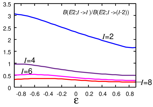
Figure 14: Dependence on the mass-asymmetry parameter $\epsilon$ of the ratios $B(E2;I_{\rm yrare}\rightarrow I_{\rm yrast})/B(E2;I_{\rm yrare}\rightarrow(I-2)_{\rm yrare})$, calculated for $V_{0}=1.0$ and $V_{1}=0.5$ MeV. Here, $I_{\rm yrast}$ and $I_{\rm yrare}$ denote the yrast and the yrare states having the same values of angular momenta $I$, while $(I-2)_{\rm yrare}$ the yrare states with angular momentum $I-2$.

Due to the two peak structure of the yrare wave functions mentioned above, the ratios of $B(E2)$ values from an yrare state to an yrast state to those between the yrare states remain rather large for a wide region of the mass-asymmetry parameter $\epsilon$. This is shown in Fig. 14.

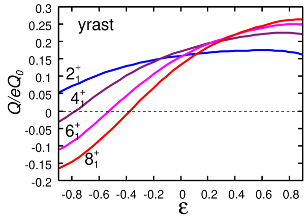
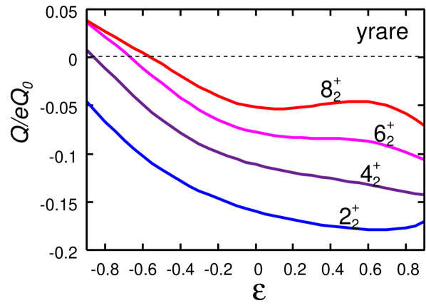
Figure 15: Dependence of the quadrupole moments on the mass-asymmetry parameter $\epsilon$, calculated for $V_{0}=1.0$ and $V_{0}=0.5$ MeV. The left and the right panels display the results of calculation for the yrast and the yrare states, respectively.

In spite of the two-peak structure of the yrare wave functions, we can find a feature of shape coexistence in the spectroscopic quadrupole moments $Q$, which are shown in Fig. 15 as functions of $\epsilon$. Let us first concentrate on the $\epsilon>0$ part of this figure. We see that the $Q$ values of the yrast states are positive, indicating their oblatelike character, while the yrare states have negative $Q$, indicating their prolatelike character. This can be regarded as a feature of the shape coexistence. It is furthermore seen that the absolute magnitude of $Q$ increases as $\epsilon$ increases, except the $8_{2}^{+}$ state. As discussed above in connection with Fig. 13, for positive $\epsilon$, the oblate shape is favored to lower the rotational energy. Consequently, with $\epsilon$ increasing, the collective wave functions in the yrast band tend to localize around the oblate shape more and more and those of the yrare states localize around the prolate shape because of the orthogonality if the angular momentum is not so high.

It is also noticeable that the absolute magnitude of $Q$ in the yrare band decreases with increase in the angular momentum. This is because the cancellation mechanism between the contributions from the oblatelike and prolatelike regions of the collective wave function works more strongly as the two-peak structure grows.

Next, let us discuss on the $\epsilon<0$ part of Fig. 15. For negative $\epsilon$, the prolate shape is favored to lower the rotational energy. On the other hand, the collective potential under consideration ($V_{1}=0.5$ MeV) is lower for the oblate shape. Hence, the rotational energy and the potential energy compete to localize the collective wave function into the opposite directions. It is seen in Fig. 15 that the spectroscopic quadrupole moments of the yrast states decrease with $\epsilon$ decreasing and that this trend is stronger for higher angular momentum states. As a consequence, the $Q$ values of the $6_{1}^{+}$ and $8_{1}^{+}$ states become negative for large negative $\epsilon$, which implies that the rotational effect dominates there.

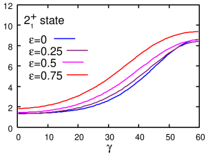
(a) $2_{1}^{+}$

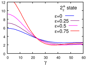
(b) $2_{2}^{+}$

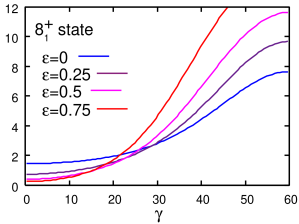
(c) $8_{1}^{+}$

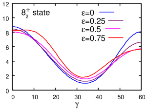
(d) $8_{2}^{+}$

Figure 16: Dependence of the collective wave functions on the mass-asymmetry parameter $\epsilon$, calculated for $V_{0}=1.0$ and $V_{1}=0.5$ MeV. The upper-left and the upper-right panels display the results of calculation for the yrast and the yrare states with $I^{\pi}=2^{+}$, while the lower-left and the lower-right panels show those for the yrast and the yrare states with $I^{\pi}=8^{+}$.

Finally, we show in Fig. 16 how the localization properties of the collective wave functions depend on the mass-asymmetry parameter $\epsilon$, taking the $2^{+}$ and $8^{+}$ states as representatives of low and high angular momentum states. It is clearly seen that, for the yrast states, while the the localization of the $2_{1}^{+}$ state around the oblate shape is rather insensitive to $\epsilon$, that of $8_{1}^{+}$ state remarkably develops with increasing $\epsilon$. For the yrare states, the localization of the $2_{2}^{+}$ state around the prolate shape grows with increasing $\epsilon$, while the $8_{2}^{+}$ state retains the two-peak structure discussed above for every value of $\epsilon$. The different effects of the mass-asymmetry parameter $\epsilon$ on the $2^{+}$ and $8^{+}$ states are comprehensible from the consideration of the relative importance of the rotational and vibrational energies shown in Table I. We see that the rotational energies dominate in the $8^{+}$ states, while the vibrational energies are comparable in magnitude to the rotational energies in the $2^{+}$ states. Thus, the effect of the mass-asymmetry parameter $\epsilon$ on the localization properties of the $8^{+}$ states can be easily accounted by the rotational energy. On the other hand, in the situation characterized by the parameters $V_{0}=1.0$ and $V_{1}=0.5$ MeV, the properties of the $2^{+}$ states are determined by a delicate competition between the rotational and vibrational kinetic energies as well as the potential energy. The growth of the prolate peak with increasing $\epsilon$ in the $2_{2}^{+}$ state turns out due mainly to the increase of the vibrational mass $D_{\gamma\gamma}$ at the prolate shape.

Table 1: Expectation values of the vibrational and rotational energies in units of MeV for the $2_{1}^{+},2_{2}^{+},8_{1}^{+}$and $8_{2}^{+}$ states. The results for $\epsilon=0.0$ and $0.5$ are shown.

		$2_{1}^{+}$	$2_{2}^{+}$	$8_{1}^{+}$	$8_{2}^{+}$
$\epsilon=0.0$	$\langle\hat{T}_{\rm vib}\rangle$	0.23	0.42	0.35	1.09
	$\langle\hat{T}_{\rm rot}\rangle$	0.29	0.55	2.56	2.87
$\epsilon=0.5$	$\langle\hat{T}_{\rm vib}\rangle$	0.20	0.51	0.49	1.03
	$\langle\hat{T}_{\rm rot}\rangle$	0.24	0.60	2.40	3.18

Summarizing this subsection, we have found that the OP symmetry breaking in the collective mass plays an important role in developing the localization of the collective wave functions of the yrast states. On the other hand, the asymmetry of the collective mass tends to enhance the two peak structure of the yrare states.

5 Role of $\beta$-$\gamma$ couplings

In this section, we examine whether or not the results obtained in the previous section using the (1+3)D model remain valid when we take into account the $\beta$ degree of freedom. Because this is a vast subject, we here concentrate on the situation in which we are most interested: namely, the case with $V_{0}=1.0,V_{1}=0.5$ MeV and $\epsilon=0.5$.

5.1 A simple (2+3)-dimensional model

We come back to the collective Schrödinger equation (13) for the general 5D quadrupole collective Hamiltonian and set up the collective potential in the following form:

$$V(\beta,\gamma)=\frac{1}{2}C(\beta^{2}-\beta_{0}^{2})^{2}-v_{0}\beta^{6}\cos^{2}3\gamma+v_{1}\beta^{3}\cos 3\gamma+C_{6}\beta^{6},$$ (22)

where $v_{0}=V_{0}/\beta_{0}^{6}$ and $v_{1}=V_{1}/\beta_{0}^{3}$. The first term ensures that the collective wave functions localize around $\beta\simeq\beta_{0}$. The second and third terms are reduced to the collective potential $V(\gamma)$ in the (1+3)D model when the collective coordinate $\beta$ is frozen at $\beta=\beta_{0}$. The fourth term guarantees that the potential satisfies the boundary condition, $V(\beta,\gamma)\rightarrow\infty$ as $\beta\rightarrow\infty$. Obviously, the collective potential (22) fulfills the requirement that it should be a function of $\beta^{2}$ and $\beta^{3}\cos 3\gamma$. We note that various parameterizations of the collective potential similar to Eq.(22) have been used by many authors. [27, 37, 40] It is certainly interesting and possible to derive the coefficients $C,v_{0},v_{1},C_{6}$ and $\beta_{0}$ using microscopic theories of nuclear collective motion. In this paper, however, we simply treat these coefficients as phenomenological parameters and determine these values so that the resulting collective potential $V(\beta,\gamma)$ qualitatively simulates that obtained using the microscopic HFB calculation [53] for ⁶⁸Se . They are $C=800,~{}V_{0}=1.0,~{}V_{1}=0.5,~{}C_{6}=1000$ MeV and $\beta_{0}^{2}=0.1$. In Fig. 17, the collective potential with these coefficients is drawn in the $(\beta,\gamma$) plane. One may immediately notice the following characteristic features of this collective potential. 1) There are two local minima, one at the oblate shape and the other at the prolate shape. They are approximately degenerate in energy but the oblate minimum is slightly lower. 2) There is a valley along the $\beta=\beta_{0}$ line connecting the two local minima. 3) The spherical shape is a local maximum, which is approximately 4 MeV higher than the oblate minimum.

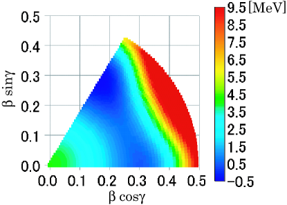
Figure 17: Map of the two-dimensional collective potential $V(\beta,\gamma)$ defined by Eq. (22) for $C=800.0,~{}V_{0}=1.0,~{}V_{1}=0.5,~{}C_{6}=1000.0$ MeV and $\beta_{0}^{2}=0.1$.

We set up the collective mass functions appearing in the collective kinetic energy terms as follows:

$$D_{\beta\beta}(\beta,\gamma) =D(1-\epsilon^{\prime}\beta\cos 3\gamma),$$ (23)

$$D_{\gamma\gamma}(\beta,\gamma) =D\beta^{2}(1+\epsilon^{\prime}\beta\cos 3\gamma),$$ (24)

$$D_{\beta\gamma}(\beta,\gamma) =D\epsilon^{\prime}\beta\sin 3\gamma,$$ (25)

$$D_{k}(\beta,\gamma) =D(1+\epsilon^{\prime}\beta\cos\gamma_{k}),$$ (26)

where $\epsilon^{\prime}=\epsilon/\beta_{0}$. These expressions are adopted to take into account the lowest-order $(\beta,\gamma)$ dependence of the collective mass functions derived by Yamada [48] by means of the SCC method. [51] We use the same values for $D$ and $\epsilon$ as in Fig. 13, namely $D$=50MeV^-1 and $\epsilon=0.5$.

5.2 Comparison of the (1+3)D and the (2+3)D model calculations

We have solved the collective Schrödinger equation (13) using the collective potential (22) and the collective masses (23)-(26). Below, the results of the numerical calculation are presented and compared with those of the (1+3)D model.

Figures 18 and 19 display on the ($\beta,\gamma$) plane the two-dimensional collective wave functions squared, $\sum_{K}|\Phi_{IK\alpha}(\beta,\gamma)|^{2}$, and the $\beta^{4}$-weighted ones, $\beta^{4}\sum_{K}|\Phi_{IK\alpha}(\beta,\gamma)|^{2}$, respectively, of the yrast and yrare states with even angular momenta $I=0-8$. The $\beta^{4}$ factor carries the major $\beta$ dependence of the intrinsic volume element $d\tau^{\prime}$ given by Eq. (17). We see in Fig. 18 that, except the $0^{+}$ states, the yrast (yrare) wave functions are well localized around the oblate (prolate) shape. While the localization of the yrast wave functions grows as the angular momentum increases, the yrare wave functions gradually develop the second peaks around the oblate shape. These behaviors are qualitatively the same as those we have seen for the collective wave functions in the (1+3)D model in Fig. 13. For the $0^{+}$ states, the wave functions squared in Fig. 18 appear to be spread over a rather wide region around the spherical shape, but the $\beta^{4}$-weighted ones in Fig. 19 take the maxima (as functions of $\beta$) near the constant-$\beta$ line with $\beta=\beta_{0}$. Thus, we can see in Fig. 19 a very good correspondence with the (1+3)D wave functions including the $0^{+}$ states also. That is, the behaviors along the constant-$\beta$ line of the collective wave functions in the (2+3)D model exhibit qualitatively the same features as those of the (1+3)D model. (A minor difference is seen only in the relative heights of the oblate and prolate peaks of the $0_{2}^{+}$ wave function.) We note that the localization properties of the collective wave function are seen better in the $\beta^{4}$-weighted wave functions squared than those multiplied by the total intrinsic volume element, $d\tau^{\prime}\sum_{K}|\Phi_{IK\alpha}(\beta,\gamma)|^{2}$, which always vanish at the oblate and prolate shapes due to the $\sin 3\gamma$ factor contained in $d\tau^{\prime}$.

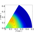
(a) $0_{1}$ state

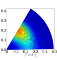
(b) $2_{1}$ state

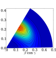
(c) $4_{1}$ state

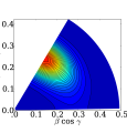
(d) $6_{1}$ state

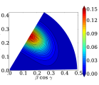
(e) $8_{1}$ state

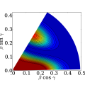
(f) $0_{2}$ state

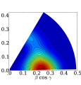
(g) $2_{2}$ state

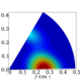
(h) $4_{2}$ state

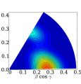
(i) $6_{2}$ state

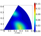
(j) $8_{2}$ state

Figure 18: Collective wave functions squared $\sum_{K}|\Phi_{IK\alpha}(\beta,\gamma)|^{2}$ calculated for the mass-asymmetry parameter $\epsilon=0.5$ and the two-dimensional collective potential $V(\beta,\gamma)$ with $C=800.0,V_{0}=1.0,~{}V_{1}=0.5,~{}C_{6}=1000.0$ MeV and $\beta_{0}^{2}=0.1$. The upper and the lower panels display the results for the yrast and the yrare states, respectively.

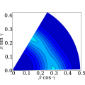
(a) $0_{1}$ state

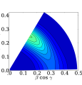
(b) $2_{1}$ state

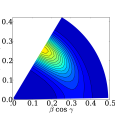
(c) $4_{1}$ state

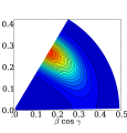
(d) $6_{1}$ state

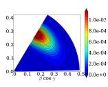
(e) $8_{1}$ state

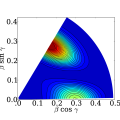
(f) $0_{2}$ state

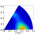
(g) $2_{2}$ state

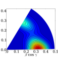
(h) $4_{2}$ state

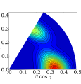
(i) $6_{2}$ state

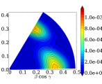
(j) $8_{2}$ state

Figure 19: The same as Fig. 18 but for weighted collective wave functions squared $\beta^{4}\sum_{K}|\Phi_{IK\alpha}(\beta,\gamma)|^{2}$.

Finally we compare in Fig. 20 the excitation spectrum obtained in the (2+3)D model with that in the (1+3)D model. It is evident that they agree very well. Aside from the quantitative difference that the excitation energies are a little higher and the $B(E2)$ values increase more rapidly with increase in the angular momentum in the (2+3)D model than in the (1+3)D model, the essential features of the excitation spectrum are the same. In particular, we find a beautiful agreement in the level sequences: the energy ordering of these eigenstates are exactly the same between the two calculations. This agreement implies that the $\beta$-$\gamma$ coupling plays only a secondary role here, and the major feature of the excitation spectrum is determined by triaxial deformation dynamics. In this dynamics, the $\gamma$ dependence of the collective mass functions plays an important role as well as that of the collective potential.

The excitation spectra of Fig. 20 are quite different from any of the patterns known well in axially symmetric deformed nuclei, in the rigid triaxial rotor model and in the $\gamma$-unstable model. It also deviates considerably from the spectrum expected in an ideal situation of the oblate-prolate shape coexistence where two rotational bands keep their identities without strong mixing between them. Among a number of interesting features, we first notice the unique character of the $0_{2}^{+}$ state. It is significantly shifted up in energy from its position expected when the yrare $0_{2}^{+},2_{2}^{+},4_{2}^{+},6_{2}^{+}$ and $8_{2}^{+}$ states form a regular rotational band. As we have discussed in connection with Fig. 3, the position of the $0_{2}^{+}$ state relative to the $2_{2}^{+}$ state serves as a sensitive measure indicating where the system locates between the $\gamma$-unstable situation ($V_{0}=V_{1}=0$) and the ideal oblate-prolate shape coexistence (large $V_{0}$ and small $V_{1}$). Thus, the results of our calculation suggest that experimental data for the excitation energy of the $0_{2}^{+}$ state provide very valuable information on the barrier height between the oblate and prolate local minima. In this connection, we also note that the $3_{1}^{+}$ ($5_{1}^{+}$) state is situated slightly higher in energy than the $6_{1}^{+}$ and $4_{2}^{+}$ ($8_{1}^{+}$ and $6_{2}^{+}$) states. These are other indicators suggesting that the system is located in an intermediate situation between the two limits mentioned above.

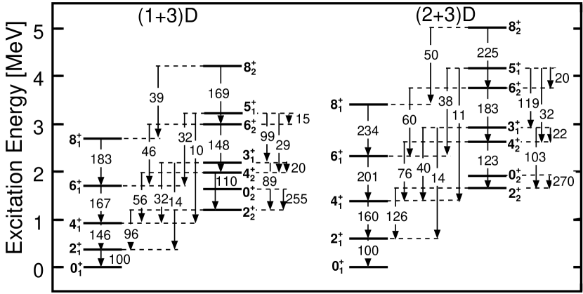
Figure 20: Comparison of the excitation spectra and the $E2$-transition properties in the (1+3)D model (left side) and those in the (2+3)D model (right side), calculated for the potential parameters $V_{0}=1.0,V_{1}=0.5$ MeV and the mass-asymmetry parameter $\epsilon=0.5$. Additional parameters for the two-dimensional potential $V(\beta,\gamma)$ in the (2+3)D model are $C=800.0$ and $C_{6}=1000.0$ MeV. The $B(E2)$ values are written on the transition arrows normalizing $B(E2;2_{1}\rightarrow 0_{1})$ as 100. Weak $E2$ transitions whose $B(E2)$ values smaller than 10 are not shown.

In Fig. 20, we furthermore notice interesting properties of the $E2$ transitions from the yrare to the yrast states: for instance, the $E2$ transitions with $\Delta I=-2$, or $B(E2;I_{\rm yrare}\rightarrow(I-2)_{\rm yrast})$, and those with $\Delta I=+2$, or $B(E2;I\rightarrow(I+2)_{\rm yrast})$, are much smaller than other yrare-to-yrast $E2$ transitions. These transitions are forbidden in the $\gamma$-unstable model [16] because they transfer the boson seniority $v$ by $\Delta v=2$ and $\Delta v=0$, respectively. Thus, some features characteristic to the $\gamma$-unstable situation persist here. On the other hand, although $B(E2;3_{1}\rightarrow 4_{2})$ and $B(E2;5_{1}\rightarrow 6_{2})$ are also forbidden transitions with $\Delta v=0$ in the $\gamma$-unstable limit, they are not very small in Fig. 20 and indicate a significant deviation from the $\gamma$-unstable limit.

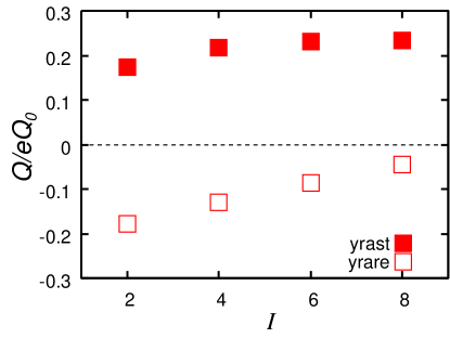
(a) (1+3)D

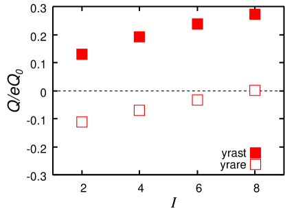
(b) (2+3)D

Figure 21: The same as Fig. 20 but for the spectroscopic quadrupole moments in units of the intrinsic quadrupole moment, $eQ_{0}=3e/\sqrt{5\pi}ZR_{0}^{2}\beta_{0}$. The results of calculation in the (1+3)D model and in the (2+3)D model are displayed as functions of angular momentum $I$ in the left and right panels, respectively. The values for the yrast (yrare) states are shown by filled (open) squares.

The spectroscopic quadrupole moments $Q$ calculated in the (1+3)D and the (2+3)D models are compared in Fig. 21. It is seen again that the two calculations show the same qualitative features: both calculations yield the positive (negative) sign for the spectroscopic quadrupole moments of the yrast (yrare) states to indicate an oblatelike (prolatelike) character. Quantitatively, in the (2+3)D model, the yrast $Q$ value increases with angular momentum more significantly and the absolute values of the yrare $Q$ moments are slightly smaller than those of the (1+3)D model. As we discussed above, in both calculations, the $Q$ value of the yrare states approaches zero with the angular momentum increasing due to the cancellation mechanism associated with the growth of the two peak structure in the collective wave functions. In spite of such deviations from a simple picture, we can see in Fig. 21 some qualitative features characteristic to the oblate-prolate shape coexistence.

We conclude that the excitation spectrum and the properties of the quadrupole transitions and moments exhibited in Figs. 20 and 21 can be regarded as those characteristic to an intermediate situation between the well-developed oblate-prolate shape coexistence and the $\gamma$-unstable limit.

6 Concluding Remarks

From a viewpoint of the oblate-prolate symmetry and its breaking, we have proposed a simple (1+3)D model capable of describing the coupled motion of the large-amplitude shape fluctuation in the $\gamma$-degree of freedom and the three-dimensional rotation. Using this model, we have made a systematic investigation of the oblate-prolate shape coexistence phenomena and their relationships to other classes of low-frequency quadrupole modes of excitation, including particular cases described by the $\gamma$-unstable model and the rigid triaxial rotor model. We have also adopted the (2+3)D model to check the validity of freezing the $\beta$ degree of freedom in the (1+3)D model. We have obtained a number of interesting suggestions for the properties of low-lying states that are characteristic to an intermediate situation between the well-developed oblate-prolate shape-coexistence and $\gamma$-unstable limits. In particular, 1) the relative energies of the excited $0^{+}$ states can be indicators of the barrier height of the collective potential. 2) Specific $E2$ transition probabilities are sensitive to the oblate-prolate symmetry breaking. 3) Nuclear rotation can assist the localization of the collective wave functions in the $(\beta,\gamma)$ deformation space. However, even if the rotation-assisted localization is realized in the yrast band, it is not necessarily in the yrare band: the two-peak structure may develop in the yrare band.

References

- [1] S. M. Fischer et al., Phys. Rev. Lett. 84 (2000), 4064.
- [2] S. M. Fischer et al., Phys. Rev. C 67 (2003), 064318.
- [3] J. Ljungvall et al., Phys. Rev. Lett. 100 (2008), 102502.
- [4] J. L. Wood, K. Heyde, W. Nazarewicz, M. Huyse and P. van Duppen, Phys. Rep. 215 (1992), 101.
- [5] A. N. Andreyev et al., Nature 405 (2000), 430.
- [6] T. Duget, M. Bender, P. Bonche and P.-H. Heenen, \PLB559,2003,201.
- [7] R. R. Rodríguez-Guzmán , J. L. Egido and L. M. Robledo, Phys. Rev. C 69 (2004), 054319.
- [8] M. Matsuo, T. Nakatsukasa and K. Matsuyanagi, Prog. Theor. Phys. 103 (2000), 959.
- [9] M. Kobayasi, T. Nakatsukasa, M. Matsuo and K. Matsuyanagi, Prog. Theor. Phys. 113 (2005), 129.
- [10] T. Nikšić, Z. P. Li, D. Vretenar, L. Próchniak, J. Meng and P. Ring, Phys. Rev. C 79 (2009), 034303.
- [11] Z. P. Li, T. Nikšić, D. Vretenar, J. Meng, G. A. Lalazissis and P. Ring, Phys. Rev. C 79 (2009), 054301.
- [12] M. Bender and P.-H. Heenen, Phys. Rev. C 78 (2008), 024309.
- [13] M. Girod, J.-P. Delaroche, A. Görgen and A. Obertelli, Phys. Lett. B 676 (2009), 39.
- [14] N. Hinohara, T. Nakatsukasa, M. Matsuo and K. Matsuyanagi, Prog. Theor. Phys. 119 (2008), 59; Prog. Theor. Phys. 117 (2007), 451.
- [15] N. Hinohara, T. Nakatsukasa, M. Matsuo and K. Matsuyanagi, Phys. Rev. C 80 (2009), 014305.
- [16] L. Wilets and M. Jean, Phys. Rev. 102 (1956), 788.
- [17] A. S. Davydov and G. F. Filippov, Nucl. Phys. 8 (1958), 237.
- [18] A. Bohr and B. R. Mottelson, Nuclear Structure, Vol. II (W. A. Benjamin Inc., 1975; World Scientific, 1998).
- [19] A. Bohr, Mat. Fys. Medd. Dan. Vid. Selsk. 26, No. 14 (1952).
- [20] A. Bohr and B. R. Mottelson, Mat. Fys. Medd. Dan. Vid. Selsk. 27, No. 16 (1953).
- [21] G. Gneuss and W. Greiner, Nucl.Phys. 171 (1971), 449.
- [22] P. O. Hess, M. Seiwert, J. Maruhn and W. Greiner, Z. Phys. A 296 (1980), 147.
- [23] J. Libert and P. Quentin, Z. Phys. A 306 (1982), 315.
- [24] D. Troltenier, J. Maruhn, W. Greiner and P. O. Hess, Z. Phys. A 343, (1992) 25.
- [25] T. Marumori, M. Yamamura and H. Bando, Prog. Theor. Phys. 28 (1962), 87.
- [26] S. T. Belyaev, Nucl. Phys. 64 (1965), 17.
- [27] K. Kumar and M. Baranger, Nucl. Phys. A 92 (1967), 608.
- [28] K. Kumar, Nucl. Phys. A 92 (1967), 653; Nucl. Phys. A 231 (1974), 189.
- [29] M. Baranger and K. Kumar, Nucl. Phys. 62 (1965), 113; Nucl. Phys. A 110 (1968), 490; Nucl. Phys. A 110 (1968), 529; Nucl. Phys. A 122 (1968), 241; Nucl. Phys. A 122 (1968), 273.
- [30] I. Deloncle, J. Libert, L. Bennour and P. Quentin, Phys. Lett. B 233 (1989), 16.
- [31] S. G. Rohoziński, J. Dobaczewski, B. Nerlo-Pomorska, K. Pomorski and J. Srebrny, Nucl. Phys. A 292 (1977), 66.
- [32] L. Próchniak, K. Zajac, K. Pomorski, S. G. Rohoziński and J. Srebrny, Nucl. Phys. A 648 (1999), 181.
- [33] J. Libert, M. Girod and J.-P. Delaroche, Phys. Rev. C 60 (1999), 054301.
- [34] L. Próchniak, P. Quentin, D. Samsoen and J. Libert, Nucl. Phys. A 730 (2004), 59.
- [35] J. Srebrny et al., Nucl. Phys. A 766 (2006), 25.
- [36] D. J. Rowe, Nucl. Phys. A 735 (2004), 372.
- [37] D. J. Rowe, T. A. Welsh and M. A. Caprio, Phys. Rev. C 79 (2009), 054304.
- [38] F. Iachello, Phys. Rev. Lett. 85 (2000), 3580; Phys. Rev. Lett. 87 (2001), 052502; Phys. Rev. Lett. 91 (2003), 132502.
- [39] M. A. Caprio and F. Iachello, Nucl. Phys. A 781 (2007), 26.
- [40] M. A. Caprio, arXiv:0902.0022.
- [41] S. De Baerdemacker, L. Fortunato, V. Hellemans and K. Heyde, Nucl. Phys. A 769 (2006), 16.
- [42] D. Bonatsos et al., Phys. Rev. C 76 (2007), 064312.
- [43] L. Fortunato, Eur. Phys. J. A 26, s01 (2005), 1.
- [44] S. G. Lie and G. Holzwarth, Z. Phys. 249 (1972),332; Phys. Rev. C 12 (1975), 1035.
- [45] T. Tamura, K. Weeks and T. Kishimoto, Phys. Rev. C 20 (1979), 307.
- [46] K. Weeks and T. Tamura, Phys. Rev. C 22 (1980), 888; Phys. Rev. C 22 (1980), 1323.
- [47] H. Sakamoto, Phys. Rev. C 52 (1995), 177; Phys. Rev. C 64 (2001), 024303.
- [48] K. Yamada, Prog. Prog. Theor. Phys. 89 (1993), 995.
- [49] R. V. Jolos and P. von Brentano, Phys. Rev. C 79 (2009), 044310; Phys. Rev. C 78 (2008), 064309; Phys. Rev. C 77 (2008), 064317; Phys. Rev. C 76 (2007), 024309; Phys. Rev. C 74 (2006), 064307;
- [50] N. Onishi, I. Hamamoto, S. Åberg and A. Ikeda, Nucl. Phys. A 452 (1986), 71.
- [51] T. Marumori, T. Maskawa, F. Sakata and A. Kuriyama, Prog. Theor. Phys. 64 (1980), 1294.
- [52] L. D. Landau and E. M. Lifschitz, Quantum Mechanics (Non-relativistic Theory) (Pergamon Press, 1958).
- [53] M. Yamagami, K. Matsuyanagi and M. Matsuo, Nucl. Phys. A 693 (2001), 579.