Influence of detector motion in entanglement measurements with photons

Abstract

We investigate how the polarization correlations of entangled photons described by wave packets are modified when measured by moving detectors. For this purpose, we analyze the Clauser-Horne-Shimony-Holt Bell inequality as a function of the apparatus velocity. Our analysis is motivated by future experiments with entangled photons designed to use satellites. This is a first step towards the implementation of quantum information protocols in a global scale.

Entanglement plays a central role in quantum theory being one of its most distinguishing features emaranhamento1 ; emaranhamento2 . It allows for the proof that no theory of local hidden variables can ever reproduce all of the predictions of quantum mechanics Bell1 . As for applications, entanglement is crucial to quantum cryptography cripto1 ; cripto2 ; cripto3 , teleportation tele1 , dense coding densecoding1 and to the conception of quantum computers (see, e.g., Refs. comp0 ; comp2 and references therein). Currently, there is much interest in testing quantum mechanics for large space distances and eventually in implementing quantum information protocols in global scales freespace0a ; freespace0b ; freespace1 ; freespace2 ; freespace3 . Photons seem to be the ideal physical objects for this purpose. Since present technology limits the use of fiber optics in this context up to about 100 km fiber , the most viable alternative to go beyond happens to be free-space transmission using satellites and ground stations satellite1 ; satellite4 ; satellite5 . Here, rather than discussing the paramount technical challenges related to these experiments, we focus on an intrinsic physical restriction posed by the motion of the satellites when special relativity is taken into consideration. We address this issue by investigating the Clauser-Horne-Shimony-Holt (CHSH) Bell inequality CHSH69 for two entangled photons when one of the detectors is boosted with some velocity. Hereafter we assume $\hbar=c=1$ unless stated otherwise.

Let us assume a system composed of two photons, $A$ and $B$, as emitted in opposite directions along the $z$ axis in a SPS cascade peres95 . The polarization of photons $A$ and $B$ is measured along arbitrary directions as defined by the unit vectors $\hat{\bf a}_{i}$ and $\hat{\bf b}_{j}$ ($i,j=1,2$), respectively, which are orthogonal to the $z$ axis. The distance between the two detectors is large enough to make both measurements causally disconnected. It is well known that the CHSH Bell inequality

$$|E(\hat{\bf a}_{2},\hat{\bf b}_{1})+E(\hat{\bf a}_{2},\hat{\bf b}_{2})+E(\hat{\bf a}_{1},\hat{\bf b}_{1})-E(\hat{\bf a}_{1},\hat{\bf b}_{2})|\leq 2$$ (1)

is satisfied for local hidden variable theories. Here

$$E(\hat{\bf a}_{i},\hat{\bf b}_{j})\equiv\lim_{N\to\infty}\frac{1}{N}\sum_{n=1}^{N}P^{A}(\hat{\bf a}_{i})P^{B}(\hat{\bf b}_{j})$$ (2)

is the polarization correlation function obtained after an arbitrarily large number $N$ of experiments is performed, and $P^{A}(\hat{\bf a}_{i})$ assume $+1$ or $-1$ values depending on whether the polarization of photon $A$ is measured along $\hat{\bf a}_{i}$ or orthogonally to it, respectively, and analogously for $P^{B}(\hat{\bf b}_{j})$.

Now, we investigate inequality (1) in the context of quantum mechanics when we allow one of the detectors to move along the $z$ axis (say, carried by a satellite). Let us write the normalized state of a two-photon system as PT03 ; LT05

$$|\psi\rangle=\sum_{s_{A},s_{B}}\int d^{3}{k}_{A}d^{3}{k}_{B}\,\psi_{s_{A}s_{B}}(\mathbf{k}_{A},\mathbf{k}_{B})|{\bf k}_{A},{\bf\hat{\epsilon}}^{s_{A}}_{{\bf k}_{A}}\rangle|{\bf k}_{B},{\bf\hat{\epsilon}}^{s_{B}}_{{\bf k}_{B}}\rangle$$ (3)

where

$$\langle{\bf k^{\prime}}_{X}|{\bf k}_{X}\rangle=\delta(\mathbf{k^{\prime}}_{X}-\mathbf{k}_{X}),\;\;\;\;\langle{\bf\hat{\epsilon}}^{s_{X}}_{{\bf k}_{X}}|{\bf\hat{\epsilon}}^{s^{\prime}_{X}}_{{\bf k}_{X}}\rangle=\delta_{s_{X},s^{\prime}_{X}},$$

and

$$\sum_{s_{A},s_{B}}\int d^{3}{k}_{A}d^{3}{k}_{B}|\psi_{s_{A}s_{B}}(\mathbf{k}_{A},\mathbf{k}_{B})|^{2}=1.$$ (4)

Here, $X=A,B$ distinguishes between both particles, $k_{X}=(\left\|\mathbf{k}_{X}\right\|,\mathbf{k}_{X})$ are the corresponding four-momenta, and $s_{X}=\pm 1$ labels two orthogonal helicity eigenstates $|{\bf\hat{\epsilon}}^{s_{X}}_{{\bf k}_{X}}\rangle$ for fixed three-momentum ${\bf k}_{X}$. We note that $|{\bf\hat{\epsilon}}^{s_{X}}_{{\bf k}_{X}}\rangle$ is associated with the complex three-vector

$${\bf\hat{\epsilon}}^{s_{X}}_{{\bf k}_{X}}=R(\hat{\bf k}_{X}){\bf\hat{\epsilon}}^{s_{X}}_{z},$$ (5)

where ${\bf\hat{\epsilon}}^{s_{X}}_{z}\equiv(1/\sqrt{2})(1,is_{X},0)$ are orthonormal vectors in the $x\bot y$ plane and $R(\hat{\bf k}_{X})$ is the matrix which rotates $\hat{\bf z}=(0,0,1)$ into

$$\hat{{\bf k}}_{X}={\bf k}_{X}/\|{\bf k}_{X}\|\equiv(\sin\theta\cos\phi,\sin\theta\sin\phi,\cos\theta)$$

with $\theta,\phi$ being the usual spherical angles. Next, by using $|{\bf\hat{\epsilon}}^{s_{X}}_{{\bf k}_{X}}\rangle$, we define a new pair of normalized states PT03

$$|{\hat{\bf e}}_{x}({\bf k}_{X})\rangle=\frac{x_{+}({\bf k}_{X})|{\bf\hat{\epsilon}}^{+}_{{\bf k}_{X}}\rangle+x_{-}({\bf k}_{X})|{\bf\hat{\epsilon}}^{-}_{{\bf k}_{X}}\rangle}{[|x_{+}({\bf k}_{X})|^{2}+|x_{-}({\bf k}_{X})|^{2}]^{1/2}},$$ (6)

and

$$|{\hat{\bf e}}_{y}({{\bf k}_{X}})\rangle=\frac{y_{+}({\bf k}_{X})|{\bf\hat{\epsilon}}^{+}_{{\bf k}_{X}}\rangle+y_{-}({\bf k}_{X})|{\bf\hat{\epsilon}}^{-}_{{\bf k}_{X}}\rangle}{[|y_{+}({\bf k}_{X})|^{2}+|y_{-}({\bf k}_{X})|^{2}]^{1/2}},$$ (7)

associated with the unit three-vectors $\hat{\bf e}_{x}({\bf k}_{X})$ and $\hat{\bf e}_{y}({\bf k}_{X})$ which (i) are the closest ones to $\hat{\bf x}=(1,0,0)$ and $\hat{\bf y}=(0,1,0)$, respectively, and (ii) are contained in the plane orthogonal to ${\bf k}_{X}$. Here

$$x_{\pm}({\bf k}_{X})\equiv\frac{1}{\sqrt{2}}(\cos\theta\cos\phi\pm i\sin\phi),$$ (8)

$$y_{\pm}({\bf k}_{X})\equiv\frac{1}{\sqrt{2}}(\cos\theta\sin\phi\mp i\cos\phi),$$ (9)

and we note that $\hat{\bf e}_{x}({\bf k}_{X})$ and $\hat{\bf e}_{y}({\bf k}_{X})$ do not have to be mutually orthogonal. By using Eqs. (6)-(7), the horizontal and vertical polarization states can be defined as

$$|H_{X}\rangle=\int d^{3}k_{X}f_{{\bf p}_{X}}({\bf k}_{X})|{\bf k}_{X},{\hat{\bf e}}_{x}({{\bf k}_{X}})\rangle$$ (10)

and

$$|V_{X}\rangle=\int d^{3}k_{X}f_{{\bf p}_{X}}({\bf k}_{X})|{\bf k}_{X},{\hat{\bf e}}_{y}({{\bf k}_{X}})\rangle,$$ (11)

respectively, where the function $f_{{\bf p}_{X}}({\bf k}_{X})$ gives the photon momentum dispersion. By imposing that the dispersion is restricted to the $x\bot y$ plane and described by a Gaussian function, we write

$$|f_{\mathbf{p}_{X}}(\mathbf{k}_{X})|^{2}=\pi^{-1}w^{-2}\delta(k^{z}_{X}-p_{X}^{z})e^{-(k^{r}_{X}/w)^{2}}\;\;(w>0),$$ (12)

where $k^{r}_{X}\equiv\sqrt{(k^{x}_{X})^{2}+(k^{y}_{X})^{2}\,}$ and we assume that $\mathbf{p}_{A}=-\mathbf{p}_{B}=(0,0,|p|)$ since photons $A$ and $B$ move in opposite directions along the $z$ axis.

Let us now assume that our two-photon entangled system is prepared in the state

$$|\psi\rangle=\frac{1}{\sqrt{2}}(|H_{A}\rangle\otimes|H_{B}\rangle+|V_{A}\rangle\otimes|V_{B}\rangle)$$ (13)

and investigate the polarization correlations when the detector that measures, say, photon $A$ is carried by a satellite with three-velocity ${\bf v}=(0,0,v)$, while the other one, which measures photon $B$, lies at rest at the ground station. This is important to note that each detector will see the state $|\psi\rangle$ in their proper frames unitarily transformed as H68 ; W96

$$|\psi\rangle\to|\psi^{\prime}\rangle=U_{A}(\Lambda)\otimes I_{B}|\psi\rangle,$$ (14)

where $I_{B}$ is the identity operator which acts in the Hilbert space associated with particle $B$ and

$$U_{A}(\Lambda)|{\bf k}_{A},{\bf\hat{\epsilon}}^{s_{A}}_{{\bf k}_{A}}\rangle=[(\Lambda\ k_{A})^{0}/k_{A}^{0}]^{{1}/{2}}$$

$$\times\sum_{s^{\prime}_{A}=\pm 1}D_{s^{\prime}_{A}s_{A}}(\Lambda,{\bf k}_{A})|\Lambda{\bf k}_{A},{\bf\hat{\epsilon}}^{s^{\prime}_{A}}_{\Lambda{\bf k}_{A}}\rangle.$$ (15)

Here

$$D_{s^{\prime}_{A}s_{A}}(\Lambda,{\bf k}_{A})=\exp{[-is^{\prime}_{A}\Theta(\Lambda,{\bf k}_{A})]}\delta_{s^{\prime}_{A}s_{A}}$$ (16)

is the Wigner rotation, where $\Theta(\Lambda,{\bf k}_{A})$ is a phase factor GBA03 ; LPT03 . We note that ${\Lambda{\bf k}_{A}}$ denotes the spatial part of the four-vector ${\Lambda k_{A}}$. For our particular choice where the satellite moves along the $z$ direction with velocity $v$, the corresponding boost matrix $\Lambda$ is

$$\Lambda_{\cal Z}=\left(\begin{array}[]{cccc}\cosh\alpha&0&0&\sinh\alpha\\ 0&1&0&0\\ 0&0&1&0\\ \sinh\alpha&0&0&\cosh\alpha\\ \end{array}\right)$$

with $\alpha\equiv-\tanh^{-1}v,$ in which case $\Theta(\Lambda_{\cal Z},{\bf k}_{A})=0$. By using Eqs. (13), (14) and (15), we obtain

$$|\psi^{\prime}\rangle=\frac{1}{\sqrt{2}}(|H^{\prime}_{A}\rangle\otimes|H_{B}\rangle+|V^{\prime}_{A}\rangle\otimes|V_{B}\rangle),$$ (17)

where

$$|H^{\prime}_{A}\rangle=\int d^{3}k_{A}\sqrt{{([{\Lambda_{\cal Z}}}]^{-1}k_{A})^{0}/k_{A}^{0}}\;f_{{\bf p}_{A}}([{{\Lambda_{\cal Z}}}]^{-1}{\bf k}_{A})$$

$$\times\frac{x_{+}([{{\Lambda}_{\cal Z}}]^{-1}{\bf k}_{A})|{\bf k}_{A},{\bf\hat{\epsilon}}^{+}_{{\bf k}_{A}}\rangle+x_{-}([{\Lambda_{\cal Z}]^{-1}}{\bf k}_{A})|{\bf k}_{A},{\bf\hat{\epsilon}}^{-}_{{\bf k}_{A}}\rangle}{[|x_{+}([{{\Lambda_{\cal Z}}}]^{-1}{\bf k}_{A})|^{2}+|x_{-}([{{\Lambda}_{\cal Z}}]^{-1}{\bf k}_{A})|^{2}]^{1/2}},$$

(18)

$$|V^{\prime}_{A}\rangle=\int d^{3}k_{A}\sqrt{{([{\Lambda}_{\cal Z}}]^{-1}k_{A})^{0}/k_{A}^{0}}\;f_{{\bf p}_{A}}([{{\Lambda}_{\cal Z}}]^{-1}{\bf k}_{A})$$

$$\times\frac{y_{+}([{{\Lambda}_{\cal Z}}]^{-1}{\bf k}_{A})|{\bf k}_{A},{\bf\hat{\epsilon}}^{+}_{{\bf k}_{A}}\rangle+y_{-}([{\Lambda_{\cal Z}}]^{-1}{\bf k}_{A})|{\bf k}_{A},{\bf\hat{\epsilon}}^{-}_{{\bf k}_{A}}\rangle}{[|y_{+}([{\Lambda_{\cal Z}]^{-1}}{\bf k}_{A})|^{2}+|y_{-}([{{\Lambda}_{\cal Z}}]^{-1}{\bf k}_{A})|^{2}]^{1/2}}.$$

Next, we restrict the photon polarization measurements to the $x\bot y$ plane. This is convenient, hence, to define the operators

$$\!P^{X}_{xx}=|{\hat{x}_{X}}\rangle\langle{\hat{x}_{X}}|\otimes I^{X}_{\bf{k}}, P^{X}_{xy}=|{\hat{x}_{X}}\rangle\langle{\hat{y}_{X}}|\otimes I^{X}_{\bf{k}},$$ (20)

$$\!P^{X}_{yy}=|{\hat{y}_{X}}\rangle\langle{\hat{y}_{X}}|\otimes I^{X}_{\bf{k}}, P^{X}_{yx}=|{\hat{y}_{X}}\rangle\langle{\hat{x}_{X}}|\otimes I^{X}_{\bf{k}},$$ (21)

where $I^{X}_{\bf{k}}$ is the identity operator acting in the momentum space of particle $X$ and

$$|\hat{x}_{X}\rangle\equiv x_{+}({\bf k}_{X})|{\bf\hat{\epsilon}}^{+}_{{\bf k}_{X}}\rangle+x_{-}({\bf k}_{X})|{\bf\hat{\epsilon}}^{-}_{{\bf k}_{X}}\rangle+x_{l}({\bf k}_{X})|{\bf\hat{\epsilon}}^{l}_{{\bf k}_{X}}\rangle$$ (22)

and

$$|\hat{y}_{X}\rangle\equiv y_{+}({\bf k}_{X})|{\bf\hat{\epsilon}}^{+}_{{\bf k}_{X}}\rangle+y_{-}({\bf k}_{X})|{\bf\hat{\epsilon}}^{-}_{{\bf k}_{X}}\rangle+y_{l}({\bf k}_{X})|{\bf\hat{\epsilon}}^{l}_{{\bf k}_{X}}\rangle$$ (23)

are associated with the unit vectors $\hat{\bf x}=(1,0,0)$ and $\hat{\bf y}=(0,1,0)$, respectively. We recall that $x_{\pm}({\bf k}_{X})$ and $y_{\pm}({\bf k}_{X})$ are given in Eqs. (8) and (9), respectively, and $x_{l}({\bf k}_{X})\equiv\hat{\bf x}\cdot\hat{{\bf k}}_{X}$, $y_{l}({\bf k}_{X})\equiv\hat{\bf y}\cdot\hat{{\bf k}}_{X}$. In order to span a complete basis, we have introduced an unphysical longitudinal polarization state $|{\bf\hat{\epsilon}}^{l}_{{\bf k}_{X}}\rangle$ associated with the three-vector ${\bf\hat{\epsilon}}^{l}_{{\bf k}_{X}}\equiv\hat{{\bf k}}_{X}$, as in Ref. PT03 . Now, we use Eqs. (20)-(21) to introduce the operator

$$\sigma^{X}_{\varphi}=(P^{X}_{xx}-P^{X}_{yy})\cos{2\varphi}+(P^{X}_{xy}+P^{X}_{yx})\sin{2\varphi},$$ (24)

which will be useful further to compute the left-hand side of the CHSH Bell inequality (1). The eigenvalues $+1$ and $-1$ of the operator $\sigma^{X}_{\varphi}$ correspond to polarization eigenstates associated with directions tilted by angles $\varphi$ and $\varphi+\pi/2$ with respect to the $x$ axis, respectively. The correlation between the polarization measurements for the two particles $A$ and $B$ associated with directions defined by the angles $\varphi$ and $\varpi$, respectively, is given by

$$\langle\sigma^{A}_{\varphi}\otimes\sigma^{B}_{\varpi}\rangle_{\Psi}=\langle\Psi|\sigma^{A}_{\varphi}\otimes\sigma^{B}_{\varpi}|\Psi\rangle,$$ (25)

where $|\Psi\rangle$ is the state of the two-photon system.

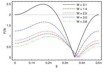
Figure 1: (Color online) $F(\vartheta)$ is plotted as a function of $\vartheta$ assuming $\alpha\to\infty$ for different values of the wave packet width properly normalized: $W=w/|p|$. The larger the wave packets the smaller the polarization correlations.

For our purposes, this is enough to consider the case where $\hat{\bf a}_{2}=\hat{\bf b}_{1}=\hat{\bf x}$. By assuming that the unit vectors $\hat{\bf a}_{1}$ and $\hat{\bf b}_{2}$ are counter-clockwisely and clockwisely rotated by an angle $\vartheta$ with respect to the $x$ axis, respectively, the left-hand side of Eq. (1)

$$F(\vartheta)\equiv|E(\hat{\bf a}_{2},\hat{\bf b}_{1})+E(\hat{\bf a}_{2},\hat{\bf b}_{2})+E(\hat{\bf a}_{1},\hat{\bf b}_{1})-E(\hat{\bf a}_{1},\hat{\bf b}_{2})|$$ (26)

is cast in the form

$$F(\vartheta)=|\langle\sigma^{A}_{0}\otimes\sigma^{B}_{0}+\sigma^{A}_{0}\otimes\sigma^{B}_{-\vartheta}+\sigma^{A}_{\vartheta}\otimes\sigma^{B}_{0}-\sigma^{A}_{\vartheta}\otimes\sigma^{B}_{-\vartheta}\rangle_{\psi^{\prime}}|,$$ (27)

where the two-photon state $|\psi^{\prime}\rangle$ is given in Eq. (17).

Next, we perform a numerical investigation of Eq. (27). As a consistency check, we have firstly verified that the standard CHSH Bell inequality, where $F(\vartheta)|_{\rm max}=2.5$, is recovered for $\alpha=0$ and $w=0$. We recall that $\alpha<0$ and $\alpha>0$ correspond to the cases where photon $A$ and the corresponding detector move towards the same and opposite directions, respectively. In Fig. 1 we exhibit how $F(\vartheta)$ is sensitive to the width of the photon wave packet properly normalized: $W\equiv w/|p|$. The plot assumes $\alpha\to\infty$ but the same pattern is verified for any other fixed $\alpha$ (including $\alpha=0$). We see that the larger the wave packet the more $|\psi\rangle$ gets mixed in polarization once momentum degrees of freedom are ignored and, thus, the smaller the polarization correlation. In Fig. 2, we plot $F(\vartheta)$ for different velocities of the moving detector assuming $W=0.6$. For large enough $|\alpha|$ ($\alpha<0$), we have that $F(\vartheta)$ is arbitrarily small in the whole domain. This shows how important the detector motion can be to polarization measurements when the velocity is high enough PST02 ; LM09 . In order to understand the pattern observed in Fig. 2, we note that as $\alpha$ decreases, photon $A$ becomes more redshifted according to the moving detector. As a consequence, $W$, which quantifies the wave dispersion normalized by the photon energy, “looks like” larger in the detection frame. Hence, from Fig. 1, $F(\vartheta)$ should indeed drop as $\alpha$ decreases. In Fig. 3, we plot $\Delta F(\vartheta)=F(\vartheta)-F_{0}(\vartheta)$, where $F_{0}(\vartheta)$ is obtained by imposing that both detectors lie at rest while realistic values are used to calculate $F(\vartheta)$: we take the mean velocity of the International Space Station, $v\approx 7.7\,\times 10^{3}{\rm m/s}$, to fix $\alpha=2.6\,\times 10^{-5}$ and present technology for the production of entangled photons to fix $W=10^{-3}$ width .

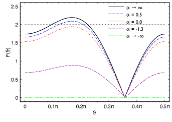
Figure 2: (Color online) $F(\vartheta)$ is plotted as a function of $\vartheta$ with $W=0.6$ for different values of the apparatus velocity. Note that $F(\vartheta)$ drops as $\alpha$ decreases.

Theoretical studies on the influence of the detector velocity in entanglement measurements is demanded by new perspectives of using satellites in quantum information experiments. Some laboratory effort to verify the influence of the detector motion in Bell inequalities using photons can be found in the literature. In Ref. SGZS02 , Stefanov, Zbinden, Ginsin and Suarez used an energy-time entangled photon pair state finding no signal for the influence of the detector motion in their results. Although we cannot make any positive statement about their results because we assume a distinct entangled state here, this is quite fair to expect from Figs. 2 and 3 that any signal of the detector velocity would only be obvious for very relativistic systems. Furthermore, Fig. 1 shows that the influence of the detector motion may be quite damped by using sharp enough wave packets ($W\ll 1$). In particular, for $w=0$ the detector velocity has no influence at all in $F(\vartheta)$. Incidentally, this may be an useful information for future applications of quantum protocols in a global scale. Although for present technology, detector motion effects should not play a dominant role as suggested by Fig. 3, this will not be probably the case in the future when more precision will be attained. This is worthwhile to recall that the Global Positioning System would not work if the tiny desynchronization between satellite and ground antennas were not corrected by General Relativity formulas A03 derived 80 years earlier.

Figure 3: (Color online) The graph exhibits $\Delta F(\vartheta)=F(\vartheta)-F_{0}(\vartheta)$. $F_{0}(\vartheta)$ is obtained by imposing that both detectors lie at rest, while realistic values are used to calculate $F(\vartheta)$: we take the mean velocity of the International Space Station to fix $\alpha=2.6\,\times 10^{-5}$ and present technology for the production of entangled photons to fix $W=10^{-3}$.

References

• (1) E. Schrödinger, Naturwissenschaften 23, 807 (1935).
• (2) R. Horodecki, P. Horodecki, M. Horodecki, and K. Horodecki, Rev. Mod. Phys 81, 865 (2009).
• (3) J. S. Bell, Physics 1, 195 (1964).
• (4) S. Wiesner, SIGACT News 15, 78 (1983).
• (5) C. H. Bennett and G. Brassard, in Proceedings of IEEE International Conference on Computers, Systems, and Signal Processing, Bangalore, 1984 (IEEE, New York, 1984), p. 175.
• (6) A. K. Ekert, Phys. Rev. Lett. 67, 661 (1991).
• (7) C. H. Bennett, G. Brassard, C. Crépeau, R. Jozsa, A. Peres, and W. K. Wootters, Phys. Rev. Lett. 70, 1895 (1993).
• (8) C. H. Bennett and S. J. Wiesner, Phys. Rev. Lett. 69, 2881 (1992).
• (9) A. Ekert and R. Jozsa, Rev. Mod. Phys. 68, 733 (1996).
• (10) P. Kok, W. J. Munro, K. Nemoto, T. C. Ralph, J. P. Dowling, and G. J. Milburn, Rev. Mod. Phys. 79, 135 (2007).
• (11) M. Aspelmeyer et al., Science 301, 621 (2003).
• (12) C.-Z. Peng et al., Phys. Rev. Lett 94, 150501 (2005).
• (13) K. J. Resch et al., Optics Express 13, 202 (2005).
• (14) R. Ursin et al., Nature Physics 3, 481 (2007).
• (15) A. Fedrizzi, R. Ursin, T. Herbst, M. Nespoli, R. Prevedel, T. Scheidl, F. Tiefenbacher, T. Jannewein, and A. Zeilinger, Nature Physics 5, 389 (2009).
• (16) N. Gisin, G. Ribordy, W. Tittel, and H. Zbinden, Rev. Mod. Phys 74, 145 (2002).
• (17) M. Aspelmeyer, T. Jennewein, M. Pfennigbauer, W. Leeb, and A. Zeilinger, Selected Topics in Quantum Electronics, IEEE Journal of 9, 1541 (2003).
• (18) P. Villoresi et al., New J. Phys. 10, 033038 (2008).
• (19) R. Ursin et al., Space-QUEST: Experiments with quantum entanglement in space. IAC Proc. A2.1.3 (2008). arXiv: quant-ph/0806.0945v1.
• (20) J. F. Clauser, M. A. Horne, A. Shimony, and R. A. Holt, Phys. Rev. Lett. 23, 880 (1969).
• (21) A. Peres, Quantum Theory: Concepts and Methods (Kluwer, Dordrecht, 1995).
• (22) A. Peres and D. R. Terno, J. Mod. Optics 50, 1165 (2003).
• (23) N. H. Lindner and D. R. Terno, J. Mod. Opt. 52, 1177 (2005).
• (24) F. R. Halpern, Special Relativity and Quantum Mechanics, (Prentice-Hall, Englewood Cliffs, NJ, 1968).
• (25) S. Weinberg, The Quantum Theory of Fields (Cambridge University Press, Cambridge, 1996), Vol. I.
• (26) R. M. Gingrich, A. J. Bergou, and C. Adami, Phys. Rev. A 68, 042102 (2003).
• (27) N. H. Lindner, A. Peres, and D. R. Terno, Jour. Phys. A 36, L449 (2003).
• (28) A. Peres, P. F. Scudo, and D. R. Terno, Phys. Rev. Lett. 88, 230402 (2002).
• (29) A. G. S. Landulfo and G. E. A. Matsas, Phys. Rev. A 79, 044103 (2009).
• (30) A. Fedrizzi, T. Herbst, A. Poppe, T. Jennewein, and A. Zeilinger, Optics Express 15, 15377 (2007).
• (31) A. Stefanov, H. Zbinden, N. Gisin, and A. Suarez, Phys. Rev. Lett. 88, 120404 (2002).
• (32) N. Ashby, Living Rev. Relativity 6, (2003), 1 (http:// www.livingreviews.org/lrr-2003-1).