New exact solutions with constant asymptotic values at infinity of the NVN integrable nonlinear evolution equation via $\bar{\partial}$-dressing method

Abstract

The classes of exact multi line soliton, periodic solutions and solutions with functional parameters, with constant asymptotic values at infinity $u|_{\xi^{2}+\eta^{2}\rightarrow\infty}\rightarrow-\epsilon$, for the hyperbolic and elliptic versions of the Nizhnik-Veselov-Novikov (NVN) equation via $\bar{\partial}$-dressing method of Zakharov and Manakov were constructed.

At fixed time these solutions are exactly solvable potentials correspondingly for one-dimensional perturbed telegraph and two-dimensional stationary Schrödinger equations. Physical meaning of stationary states of quantum particle in exact one line and two line soliton potential valleys was discussed.

In the limit $\epsilon\rightarrow 0$ exact special solutions $u^{(1)}$, $u^{(2)}$ (line solitons and periodic solutions) were found which sum $u^{(1)}+u^{(2)}$ (linear superposition) is also exact solution of NVN equation.

1 Introduction

Exact solutions of differential equations of mathematical physics, linear and nonlinear, are very important for the understanding of various physical phenomena. In the last three decades the Inverse Scattering Transform (IST) method has been generalized and successfully applied to several two-dimensional nonlinear evolution equations such as Kadomtsev-Petviashvili, Davey-Stewartson, Nizhnik-Veselov-Novikov, Zakharov-Manakov system, Ishimori, two-dimensional integrable Sin-Gordon and others (see books  [1]-[4] and references therein).

The extension of nonlocal Riemann-Hilbert problem by Zakharov and Manakov [5] and $\bar{\partial}$-problem approach [6] led to the discovery of more general $\bar{\partial}$-dressing method [7]-[10] which became very powerful method for solving two-dimensional integrable nonlinear evolution equations. In the present paper the $\bar{\partial}$-dressing method of Zakharov and Manakov was used for the construction of the classes of exact multisoliton and periodic solutions of the famous (2+1)-dimensional Nizhnik-Veselov-Novikov (NVN) integrable equation

$$u_{t}+\kappa_{1}u_{\xi\xi\xi}+\kappa_{2}u_{\eta\eta\eta}+3\kappa_{1}(u\partial^{-1}_{\eta}u_{\xi})_{\xi}+3\kappa_{2}(u\partial^{-1}_{\xi}u_{\eta})_{\eta}=0,$$ (1.1)

where $u(\xi,\eta,t)$ is scalar function, $\kappa_{1},\,\kappa_{2}$ are arbitrary constants, $\xi=x+\sigma y,\,\eta=x-\sigma y$, and $\sigma^{2}=\pm 1$; $\partial_{\xi}\equiv\frac{\partial}{\partial\xi},\,\partial_{\eta}\equiv\frac{\partial}{\partial\eta}$ and $\partial^{-1}_{\xi}$, $\partial^{-1}_{\eta}$ are operators inverse to $\partial_{\xi}$ and $\partial_{\eta}$: $\partial^{-1}_{\eta}\partial_{\eta}=\partial^{-1}_{\xi}\partial_{\xi}=1$. Equation (1.1) was first introduced and studied by Nizhnik  [11] for hyperbolic version (NVN-II equation) with $\sigma=1$ and independently by Veselov and Novikov [12] for elliptic version (NVN-I equation) with $\sigma=i$, $\kappa_{1}=\overline{\kappa}_{2}=\kappa$. The NVN equation is integrable by the IST due to representation of it as the compatibility condition for two linear auxiliary problems [11],[12]:

$$L_{1}\psi=\big{(}\partial_{\xi\eta}^{2}+u\big{)}\psi=0,$$ (1.2)

$$L_{2}\psi=\big{(}\partial_{t}+\kappa_{1}\partial_{\xi}^{3}+\kappa_{2}\partial_{\eta}^{3}+3\kappa_{1}\big{(}\partial_{\eta}^{-1}u_{\xi}\big{)}+3\kappa_{2}\big{(}\partial_{\xi}^{-1}u_{\eta}\big{)}\big{)}\psi=0$$ (1.3)

in the form of the Manakov’s triad

$$[L_{1},L_{2}]=BL_{1},\quad B=3\big{(}\kappa_{1}\partial_{\eta}^{-1}u_{\xi\xi}+\kappa_{2}\partial_{\xi}^{-1}u_{\eta\eta}\big{)}.$$ (1.4)

The present paper is the continuation of Dubrovsky et al work and follows the notations, review of the subject and general considerations presented in the previous papers [22]-[24]. We apply the $\bar{\partial}$-dressing method of Zakharov and Manakov for the construction of classes of exact solutions with non-zero constant asymptotic values at infinity:

$$u(\xi,\eta,t)=\tilde{u}(\xi,\eta,t)+u_{\infty}=\tilde{u}(\xi,\eta,t)-\epsilon,$$ (1.5)

where $\tilde{u}(\xi,\eta,t)\rightarrow 0$ as $\xi^{2}+\eta^{2}\rightarrow\infty$. In this case the first linear auxiliary problem in (1.2) has the form:

$$\big{(}\partial_{\xi\eta}^{2}+\tilde{u}\big{)}\psi=\epsilon\psi.$$ (1.6)

For $\sigma=1$ with real space variables $\xi\Rightarrow t-x,\,\eta\Rightarrow t+y$ equation (1.6) can be interpreted as perturbed telegraph equation with potential $u=\tilde{u}-\epsilon$ or perturbed string equation for $\epsilon=0$. For $\sigma=i$ with complex space variables $\xi\Rightarrow x+iy=z,\,\eta\Rightarrow x-iy=\overline{z}$ equation (1.6) coincides with the famous two-dimensional stationary Schrödinger equation

$$\big{(}-2\partial_{z\bar{z}}^{2}+V_{Schr}\big{)}\psi=E\psi$$ (1.7)

with $V_{Schr}=-2\tilde{u}$ and $E=-2\epsilon$. For this reason the construction via $\bar{\partial}$-dressing method of exact solutions of the NVN equations with constant asymptotic values at infinity means simultaneous calculation of exact eigenfunctions (wave functions) $\psi$ and exactly solvable potentials $u=\tilde{u}-\epsilon$ and $V_{Schr}=-2\tilde{u}$ for above mentioned famous linear equations.

The inverse scattering transform for the first auxiliary linear problem (1.6) (or in particular for 2D Schrödinger equation (1.7)) has been developed in a number of papers. Detailed review one can find in the book of Konopelchenko [3]. On the basis of developed for (1.6) IST using time evolution given by second auxiliary problem (1.3) several classes of exact solutions of NVN equation were constructed [3], [4],[11]-[21]. Some exact solutions of NVN-II equation with $\sigma=1$ were obtained in the work [11] via the transformation operators. Veselov et al constructed finite zone solutions of NVN equation [12]. The classes of rational localized solutions of so called $NVN-I_{\pm}$-equation (with $E>0$ and $E<0$ for (1.7)) corresponding to the case of simple poles of wave function $\psi$ were presented in the works [14]-[16]. Special care requires the case of $E=0$ for (1.7), i. e. the case of $NVN-I_{0}$ equation [17]. The use of Darbu transformations for the construction of exact solutions of NVN equation was demonstrated by Matveev et al [18]. The class of dromion-like solutions of NVN equation via Mottard transformations was constructed by Athorne et al [21]. We have already constructed classes of exact potentials for perturbed telegraph equation (1.6) with potential $u=\tilde{u}-\epsilon$ and perturbed string equation with $u=\tilde{u},\epsilon=0$ via $\overline{\partial}$-dressing method in the paper [22] and obtained some rationally localized solutions of NVN-equation with simple and multiple pole wave functions $\psi$ via $\overline{\partial}$-dressing method [23],[24].

Present work is concentrated on further use of $\overline{\partial}$-dressing method for the construction of exact solutions of two-dimensional integrable nonlinear evolution equations, exact potentials and wave functions of famous linear auxiliary problems (1.6) or (1.7) and the study of their possible applications. While many studies of this subject were performed the question of physical interpretation and exploitation of results obtained via $\overline{\partial}$-dressing are still of great interest.

The paper is organized as described further. Basic ingredients of the $\bar{\partial}$-dressing method for the NVN equation (1.1) in brief are presented in sections 2,3 and general determinant formula for multi line soliton solutions and useful formulas for the conditions of reality and potentiality of $u$ are obtained. In sections 4 and 5 the classes of exact multi line soliton solutions for hyperbolic version with $\sigma=1$ and for elliptic version with $\sigma=i$ of the NVN equation respectively are constructed. The classes of periodic solutions for both versions of NVN equation are constructed in section 6. The classes of solutions with functional parameters are constructed in section 7. The simplest examples of exact one, two line soliton solutions with corresponding exact wave functions of auxiliary linear problems, periodic solutions and solutions with functional parameters are presented in sections 3,4 and 5,6,7 of the paper.

2 Basic ingredients of the $\bar{\partial}$-dressing method and general determinant formulas for exact solutions

As a matter of convenience here we briefly reviewed the basic ingredients of the $\bar{\partial}$-dressing method [7]-[10] for the NVN equation (1.1) in the case of $u(\xi,\eta,t)$ with generically non-zero asymptotic value at infinity (1.6). We followed the treatment of the papers [23],[24] without repetition of theirs detailed calculations.

At first one postulates the non-local $\bar{\partial}$-problem:

$$\frac{\partial\chi(\lambda,\bar{\lambda})}{\partial\bar{\lambda}}=(\chi*R)(\lambda,\bar{\lambda})={\int\int}_{C}\chi(\mu,\overline{\mu})R(\mu,\overline{\mu};\lambda,\bar{\lambda})d\mu\wedge d\overline{\mu}$$ (2.1)

where in our case $\chi$ and $R$ are the scalar complex-valued functions and $\chi$ has canonical normalization: $\chi\rightarrow 1$ as $\lambda\rightarrow\infty$. It should be assumed that the problem (2.1) is unique solvable. Then one introduces the dependence of kernel $R$ of the $\bar{\partial}$-problem (2.1) on the space and time variables $\xi$,$\eta$,$t$:

$$\frac{\partial R}{\partial\xi} = i\mu R(\mu,\overline{\mu};\lambda,\overline{\lambda};\xi,\eta,t)-R(\mu,\overline{\mu};\lambda,\overline{\lambda};\xi,\eta,t)i\lambda,$$

$$\frac{\partial R}{\partial\eta} = -i\frac{\epsilon}{\mu}R(\mu,\overline{\mu};\lambda,\overline{\lambda};\xi,\eta,t)+R(\mu,\overline{\mu};\lambda,\overline{\lambda};\xi,\eta,t)i\frac{\epsilon}{\lambda},$$ (2.2)

$$\frac{\partial R}{\partial t} = i(\kappa_{1}\mu^{3}-\kappa_{2}\frac{\epsilon^{3}}{\mu^{3}})R(\mu,\overline{\mu};\lambda,\overline{\lambda};\xi,\eta,t)-R(\mu,\overline{\mu};\lambda,\overline{\lambda};\xi,\eta,t)i(\kappa_{1}\lambda^{3}-\kappa_{2}\frac{\epsilon^{3}}{\lambda^{3}}).$$

Integrating (2) one obtains

$$R(\mu,\overline{\mu};\lambda,\bar{\lambda};\xi,\eta,t)=R_{0}(\mu,\overline{\mu};\lambda,\bar{\lambda})e^{F(\mu;\xi,\eta,t)-F(\lambda;\xi,\eta,t)}$$ (2.3)

where

$$F(\lambda;\xi,\eta,t)=i\big{[}\lambda\xi-\frac{\epsilon}{\lambda}\eta+\big{(}\kappa_{1}\lambda^{3}-\kappa_{2}\frac{\epsilon^{3}}{\lambda^{3}}\big{)}t\big{]}.$$ (2.4)

By the use of ”long” derivatives

$$D_{1}=\partial_{\xi}+i\lambda,\quad D_{2}=\partial_{\eta}-i\frac{\epsilon}{\lambda},\quad D_{3}=\partial_{t}+i\Big{(}\kappa_{1}\lambda^{3}-\kappa_{2}\frac{\epsilon^{3}}{\lambda^{3}}\Big{)}$$ (2.5)

expressing the dependence (2) of kernel $R$ of the $\bar{\partial}$-problem (2.1) on the space and time variables $\xi$,$\eta$,$t$ in the following equivalent form

$$[D_{1},R]=0,\quad[D_{2},R]=0,\quad[D_{3},R]=0$$ (2.6)

one can construct the operators of auxiliary linear problems

$$\tilde{L}=\sum\limits_{l,m,n}u_{lmn}(\xi,\eta,t)D_{1}^{l}D_{2}^{m}D_{3}^{n}.$$ (2.7)

These operators must satisfy to the conditions

$$\Big{[}\frac{\partial}{\partial\overline{\lambda}},\tilde{L}\Big{]}\chi=0,\quad\tilde{L}\chi(\lambda,\overline{\lambda})|_{\lambda\rightarrow\infty}\rightarrow 0$$ (2.8)

of absence singularities at the points $\lambda=0$ and $\lambda=\infty$ of the complex plane of spectral variable $\lambda$. For such operators $\tilde{L}$ the function $\tilde{L}\chi$ obeys the same $\bar{\partial}$-equation as the function $\chi$. There are may be several operators $\tilde{L}_{i}$ of this type, by virtue of the unique solvability of (2.1) one has $\tilde{L}_{i}\chi=0$ for each of them. In considered case one constructs two such operators:

$$\tilde{L}_{1}=D_{1}D_{2}+u_{1}D_{1}+u_{2}D_{2}+u,$$ (2.9)

$$\tilde{L}_{2}=D_{3}+\kappa_{1}D_{1}^{3}+\kappa_{2}D_{2}^{3}+V_{1}D_{1}^{2}+V_{2}D_{2}^{2}+V_{3}D_{1}+V_{4}D_{2}+V.$$ (2.10)

Using the conditions (2.8) and series expansions of wave functions $\chi$ near the points $\lambda=0$ and $\lambda=\infty$

$$\chi=\chi_{0}+\chi_{1}\lambda+\chi_{2}\lambda^{2}+\ldots,\quad\chi=\chi_{\infty}+\frac{\chi_{-1}}{\lambda}+\frac{\chi_{-2}}{\lambda^{2}}+\ldots,$$ (2.11)

one obtains the reconstruction formulas for the field variables $u_{1}$,$u_{2}$ and $V_{1}$,$V_{2}$,$V_{3}$,$V_{4}$ through the coefficients $\chi_{0}$ and $\chi_{\infty}$ of expansions (2.11) (for calculation details see papers [23],[24]):

$$u_{1}=-\frac{\chi_{\infty\eta}}{\chi_{\infty}},\quad V_{1}=-3\kappa_{1}\frac{\chi_{\infty\xi}}{\chi_{\infty}};$$ (2.12)

$$u_{2}=-\frac{\chi_{0\xi}}{\chi_{0}},\quad V_{2}=-3\kappa_{2}\frac{\chi_{0\eta}}{\chi_{0}};$$ (2.13)

$$V_{3}=3i\kappa_{2}\epsilon\chi_{1\eta},\quad V_{4}=-3i\kappa_{1}\chi_{-1\xi}.$$ (2.14)

According to well known terminology the operator $\tilde{L}_{1}$ in (2.9) is pure potential operator when its first derivatives are absent. Due to canonical normalization of wave function $\chi|_{\lambda\rightarrow\infty}\rightarrow 1$ ($\chi_{\infty}=1$):

$$u_{1}=-\frac{\chi_{\infty\eta}}{\chi_{\infty}}=0,\quad V_{1}=-3\kappa_{1}\frac{\chi_{\infty\xi}}{\chi_{\infty}}=0.$$ (2.15)

For zero value of the term $u_{2}\partial_{\eta}$ in $\tilde{L}_{1}$ one must to require $\chi_{0}=const$, without restriction we can choose $\chi_{0}=1$, and then due to (2.13)

$$u_{2}=-\frac{\chi_{0\xi}}{\chi_{0}}=0,\quad V_{2}=-3\kappa_{2}\frac{\chi_{0\eta}}{\chi_{0}}=0.$$ (2.16)

Using (2.8),(2.12) - (2.16)(for calculation details see also [23],[24]) one obtains the following expressions for $V_{3}$,$V_{4}$ and $u$:

$$V_{3}=3i\kappa_{2}\epsilon\chi_{1\eta}=3\kappa_{2}\partial_{\xi}^{-1}u_{\eta},\quad V_{4}=-3i\kappa_{1}\chi_{-1\xi}=3\kappa_{1}\partial_{\eta}^{-1}u_{\xi},$$ (2.17)

$$u=-\epsilon-i\chi_{-1\eta}=-\epsilon+i\epsilon\chi_{1\xi}.$$ (2.18)

The field variable $V$ in (2.10) due to gauge freedom [25] in the present paper is chosen to be equal to zero. In terms of the wave function

$$\psi:=\chi e^{F(\lambda;\xi,\eta,t)}=\chi e^{i\big{[}\lambda\xi-\frac{\epsilon}{\lambda}\eta+\big{(}\kappa_{1}\lambda^{3}-\kappa_{2}\frac{\epsilon^{3}}{\lambda^{3}}\big{)}t\big{]}},$$ (2.19)

under the reduction $u_{1}=0$ and $u_{2}=0$ (the condition of potentiality $\tilde{L}_{1}$), one obtains from (2.9),(2.10) due to (2.8) and (2.15)-(2.17) the linear auxiliary system (1.2),(1.3) and NVN integrable nonlinear equation (1.1) as compatibility condition (1.4) of linear auxiliary problems in (1.2), (1.3).

The solution of the $\bar{\partial}$-problem (2.1) with constant normalization $\chi_{\infty}=1$ is equivalent to the solution of the following singular integral equation:

$$\chi(\lambda)=1+\int\int\limits_{C}{\frac{d{\lambda}^{\prime}\wedge d{\bar{\lambda}}^{\prime}}{2\pi i(\lambda^{\prime}-\lambda)}}\int\int\limits_{C}\chi(\mu,\bar{\mu})R(\mu,\overline{\mu};\lambda,\bar{\lambda}){d\mu\wedge d\bar{\mu}}.$$ (2.20)

From (2.20) one obtains for the coefficients $\chi_{0}$ and $\chi_{-1}$ of the series expansions (2.11) of $\chi$ the following expressions:

$$\chi_{0}=1+\int\int\limits_{C}{\frac{d{\lambda}\wedge d{\bar{\lambda}}}{2\pi i\lambda}}\int\int\limits_{C}\chi(\mu,\bar{\mu})R_{0}(\mu,\overline{\mu};\lambda,\bar{\lambda})e^{F(\mu)-F(\lambda)}{d\mu\wedge d\bar{\mu}}$$ (2.21)

and

$$\chi_{-1}=-\int\int\limits_{C}{\frac{d{\lambda}\wedge d{\bar{\lambda}}}{2\pi i}}\int\int\limits_{C}\chi(\mu,\bar{\mu})R_{0}(\mu,\overline{\mu};\lambda,\bar{\lambda})e^{F(\mu)-F(\lambda)}{d\mu\wedge d\bar{\mu}}$$ (2.22)

where $F(\lambda)$ is short notation for $F(\lambda;\xi,\eta,t)$ given by the formula (2.4). The conditions of reality $u$ and of potentiality of the operator $\tilde{L}_{1}$ give some restrictions for the kernel $R_{0}$ of the $\bar{\partial}$-problem (2.1). In the Nizhnik case ($\sigma=1,\bar{\kappa}_{1}=\kappa_{1},\bar{\kappa}_{2}=\kappa_{2}$) of the NVN equations (1.1) with real space variables $\xi=x+y$, $\eta=x-y$ the condition of reality of $u$ leads from (2.18) and (2.22) in the limit of ”weak” fields ($\chi=1$ in (2.22)) to the following restriction for the kernel $R_{0}$ of the $\bar{\partial}$ - problem:

$$R_{0}(\mu,\overline{\mu};\lambda,\overline{\lambda})=\overline{R_{0}(-\overline{\mu},-\mu;-\overline{\lambda},-\lambda)}.$$ (2.23)

For the Veselov-Novikov case ($\sigma=i,\kappa_{1}=\kappa_{2}=\kappa=\bar{\kappa}$) of the NVN equations (1.1) with complex space variables $\xi=z=x+iy$, $\eta=\bar{z}=x-iy$ the condition of reality of $u$ leads from (2.18) and (2.22) in the limit of ”weak” fields to another restriction on the kernel $R_{0}$ of the $\bar{\partial}$ - problem:

$$R_{0}(\mu,\overline{\mu};\lambda,\overline{\lambda})=\frac{\epsilon^{3}}{{|\mu|}^{2}{|\lambda|}^{2}\overline{\mu}\overline{\lambda}}\;\overline{R_{0}(-\frac{\epsilon}{\overline{\lambda}},-\frac{\epsilon}{\lambda},-\frac{\epsilon}{\overline{\mu}}-\frac{\epsilon}{\mu})}.$$ (2.24)

The potentiality condition for the operator $\tilde{L}_{1}$ in (2.9) for the choice $\chi_{0}=1$ due to (2.21) has the following form:

$$\chi_{0}-1=\int\int\limits_{C}\frac{d\lambda\wedge d\overline{\lambda}}{2\pi i\lambda}\;\int\int\limits_{C}\;\chi(\mu,\overline{\mu})\,R_{0}(\mu,\overline{\mu};\lambda,\overline{\lambda})e^{F(\mu)-F(\lambda)}d\mu\wedge d\overline{\mu}=0.$$ (2.25)

Here we obtained general formulas for multisoliton solutions corresponding to the degenerate delta-kernel $R_{0}$:

$$R_{0}(\mu,\bar{\mu};\lambda,\bar{\lambda})=\pi\sum\limits_{k}A_{k}\delta(\mu-M_{k})\delta(\lambda-\Lambda_{k}).$$ (2.26)

In this case the wave function $\chi(\lambda)$ due to (2.20) has the form:

$$\chi(\lambda)=1+2i\sum\limits_{k}\frac{A_{k}}{\Lambda_{k}-\lambda}\chi(M_{k})e^{F(M_{k})-F(\Lambda_{k})}.$$ (2.27)

The coefficient $\chi_{-1}$ due to (2.22) and (2.26) has the form:

$$\chi_{-1}=-2i\sum\limits_{k}A_{k}\chi(M_{k})e^{F(M_{k})-F(\Lambda_{k})}.$$ (2.28)

For the wave functions $\chi(M_{k})$ from (2.27) one obtains the following system of equations:

$$\sum\limits_{l}\tilde{A}_{kl}\chi(M_{l})=1,\quad\tilde{A}_{lk}=\delta_{lk}+\frac{2iA_{k}}{M_{l}-\Lambda_{k}}e^{F(M_{k})-F(\Lambda_{k})}.$$ (2.29)

Instead of matrix $\tilde{A}$ in (2.29) it is convenient to introduce matrix $A$ given by expression

$$A_{lk}=\delta_{lk}+\frac{2iA_{k}}{M_{l}-\Lambda_{k}}e^{F(M_{l})-F(\Lambda_{k})}.$$ (2.30)

Both these matrices $\tilde{A}$ in (2.29) and $A$ (7.19) are connected by the relation

$${A}_{lk}=e^{F(M_{l})}\tilde{A}_{lk}e^{-F(M_{k})}.$$ (2.31)

From (2.29) due to (2.31) one derives the expression for the wave function $\chi$ at discrete values of spectral variable:

$$\chi(M_{l})=\sum\limits_{k}\tilde{A}_{lk}^{-1}=\sum\limits_{k}e^{F(M_{k})-F(M_{l})}A_{lk}^{-1}.$$ (2.32)

As a matter of convenience hereafter we described some useful formulas for wave functions satisfying to linear auxiliary problems (1.2),(1.3). From (2.19) and (2.32) one obtains the wave function $\psi(M_{l},\xi,\eta,t)=\chi(M_{l})e^{F(M_{l})}$ at discrete points $\lambda=M_{l}$ in the space of spectral variables:

$$\psi(M_{l},\xi,\eta,t)=\chi(M_{l})e^{F(M_{l})}=\sum\limits_{k}e^{F(M_{k})}A_{lk}^{-1}.$$ (2.33)

For the wave function (2.19) at arbitrary point $\lambda$ from (2.27) - (2.32) follows the expression:

$$\psi(\lambda,\xi,\eta,t)=\chi(\lambda)e^{F(\lambda)}=\Big{[}1+2i\sum\limits_{k}\frac{A_{k}}{\Lambda_{k}-\lambda}e^{F(M_{k})-F(\Lambda_{k})}\chi(M_{k})\Big{]}e^{F(\lambda)}=$$

$$\Big{[}1+2i\sum\limits_{k,l}\frac{A_{k}}{\Lambda_{k}-\lambda}e^{-F(\Lambda_{k})}A_{kl}^{-1}e^{F(M_{l})}\Big{]}e^{F(\lambda)}.$$ (2.34)

Inserting (2.32) into (2.28) one obtains for the coefficient $\chi_{-1}$

$$\chi_{-1}=-2i\sum\limits_{k,l}A_{k}e^{F(M_{k})-F(\Lambda_{k})}e^{F(M_{l})-F(M_{k})}A_{kl}^{-1}=$$

$$=-2i\sum\limits_{k,l}A_{k}e^{F(M_{l})-F(\Lambda_{k})}A_{kl}^{-1}=i\,tr\Big{(}\frac{\partial A}{\partial\xi}A^{-1}\Big{)}.$$ (2.35)

and due to reconstruction formula $u=-\epsilon-i\chi_{-1\eta}$ the convenient determinant formula for the solution $u$ of NVN equation (1.1):

$$u=-\epsilon+\frac{\partial}{\partial\eta}tr\Big{(}\frac{\partial A}{\partial\xi}A^{-1}\Big{)}=-\epsilon+\frac{\partial^{2}}{\partial\xi\partial\eta}\ln(\det A).$$ (2.36)

Here and below useful determinant identities

$$Tr(\frac{\partial A}{\partial\xi}A^{-1})=\frac{\partial}{\partial\xi}\ln(\det A),\quad 1+trD=det(1+D)$$ (2.37)

are used; the matrix $D$ from last identity of (7.12) is degenerate with rank 1.

Potentiality condition (2.25) by the use of (2.26)-(2.32) can be transformed to the form:

$$\chi_{0}-1=-\frac{1}{2\epsilon}\sum\limits_{k,l=1}^{N}A_{kl}^{-1}B_{lk}=0$$ (2.38)

where degenerate matrix $B$ with rank 1 is defined by the formula

$$B_{lk}=-\frac{4i\epsilon}{\Lambda_{k}}A_{k}e^{F(M_{l})-F(\Lambda_{k})}.$$ (2.39)

Due to (7.12)-(7.20) potentiality condition (2.25) takes the form:

$$0=\sum\limits_{k,m=1}^{N}A_{km}^{-1}B_{mk}=tr(A^{-1}B)=det(BA^{-1}+1)-1,$$ (2.40)

here matrix $BA^{-1}$ is degenerate of rank 1 and in deriving the last equality in (7.16) the second matrix identity of (7.12) is used. Equivalently due to (7.16) the potentiality condition takes the form

$$\det(A+B)=\det{A}.$$ (2.41)

3 Fulfilment of potentiality condition. General formulas for one line and two line solitons

Formula (2.36) for exact solutions $u(\xi,\eta,t)$ of NVN equations (1.1) is effective if the reality $\bar{u}=u$ conditions (2.23),(2.24) and potentiality condition (2.25) of operator $L_{1}$ are satisfied. This is the major and the most difficult part of all constructions. Here we demonstrated how one can to fulfil the condition of potentiality (2.25) by delta-kernel with two terms:

$$R_{0}(\mu,\bar{\mu};\lambda,\bar{\lambda})=\pi\Big{(}A\delta(\mu-\mu_{1})\delta(\lambda-\lambda_{1})+B\delta(\mu-\mu_{2})\delta(\lambda-\lambda_{2})\Big{)}.$$ (3.1)

Inserting (3.1) into (2.25) one obtains in the limit of weak fields ($\chi=1$ in (2.25)):

$$\chi_{0}-1=\int\int\limits_{C}\frac{1}{2i\lambda}\Big{(}A\delta(\mu-\mu_{1})\delta(\lambda-\lambda_{1})+B\delta(\mu-\mu_{2})\delta(\lambda-\lambda_{2})\Big{)}\times$$

$$\times e^{F(\mu)-F(\lambda)}d\mu\wedge d\overline{\mu}\,d\lambda\wedge d\overline{\lambda}=2i\bigl{(}\frac{A}{\lambda_{1}}e^{F(\mu_{1})-F(\lambda_{1})}+\frac{B}{\lambda_{2}}e^{F(\mu_{2})-F(\lambda_{2})}\bigr{)}=0.$$ (3.2)

The equality (3.2) is valid if

$$F(\mu_{1})-F(\lambda_{1})=F(\mu_{2})-F(\lambda_{2}),\quad\frac{A}{\lambda_{1}}=-\frac{B}{\lambda_{2}}.$$ (3.3)

Due to the definition of $F(\lambda)=i\big{[}\lambda\xi-\frac{\epsilon}{\lambda}\eta+\big{(}\kappa_{1}\lambda^{3}-\kappa_{2}\frac{\epsilon^{3}}{\lambda^{3}}\big{)}t\big{]}$ from space-dependent part of (3.3) the system of equations follows:

$$\mu_{1}-\lambda_{1}=\mu_{2}-\lambda_{2},\quad\frac{\epsilon}{\mu_{1}}-\frac{\epsilon}{\lambda_{1}}=\frac{\epsilon}{\mu_{2}}-\frac{\epsilon}{\lambda_{2}}.$$ (3.4)

One can show that time-dependent part of (3.3) doesn’t lead to new equation and satisfies due to the system (3.4). The system (3.4) has the following solutions:

$$1)\,\mu_{1}=\lambda_{1},\;\mu_{2}=\lambda_{2};\qquad 2)\,\mu_{1}=-\lambda_{2},\;\mu_{2}=-\lambda_{1}.$$ (3.5)

The solution $\mu_{1}=\lambda_{1},\;\mu_{2}=\lambda_{2}$ corresponds to lump solution and will not be considered here, (for more information about lump solutions see [20], [21]). For the second solution $\mu_{1}=-\lambda_{2},\;\mu_{2}=-\lambda_{1}$ taking into account second relation from (3.3) one obtains:

$$\frac{A}{\lambda_{1}}=-\frac{B}{\lambda_{2}}=\frac{B}{\mu_{1}}=a,$$ (3.6)

where $a$ is some arbitrary complex constant. It is evident that to the potentiality condition (2.25) the kernel $R_{0}$ (which is the sum of expressions of the type (3.1) with parameters defined by (3.4)-(3.6))

$$R_{0}(\mu,\bar{\mu};\lambda,\bar{\lambda})=\pi\sum\limits_{k=1}^{N}\Big{[}a_{k}\lambda_{k}\delta(\mu-\mu_{k})\delta(\lambda-\lambda_{k})+a_{k}\mu_{k}\delta(\mu+\lambda_{k})\delta(\lambda+\mu_{k})\Big{]}=$$

$$=\pi\sum\limits_{k=1}^{2N}A_{k}\delta(M-M_{k})\delta(\Lambda-\Lambda_{k})$$ (3.7)

with the sets of amplitudes $A_{k}$ and spectral parameters $M_{k},\Lambda_{k}$

$$(A_{1},..,A_{2N}):=(a_{1}\lambda_{1},...,a_{N}\lambda_{N};a_{1}\mu_{1},...,a_{N}\mu_{N});$$

$$(M_{1},...,M_{2N}):=(\mu_{1},...,\mu_{N};-\lambda_{1},...,-\lambda_{N}),$$

$$(\Lambda_{1},...,\Lambda_{2N}):=(\lambda_{1},...,\lambda_{N};-\mu_{1},...,-\mu_{N})$$ (3.8)

satisfies.

In order to avoid repetition of similar calculations in the following sections we prepared some useful formulas in general position for calculating one- and two- line soliton solutions and corresponding wave functions. The determinants of matrix $A$ (7.19) with parameters (3) corresponding to the simplest kernels (3) with $N=1$ and $N=2$ have the forms:

$$1.\quad N=1:\det A=\Big{(}1+p_{1}e^{\Delta F(\mu_{1},\lambda_{1})}\Big{)}^{2};$$ (3.9)

$$2.\quad N=2:\det A=\Big{(}1+p_{1}e^{\Delta F(\mu_{1},\lambda_{1})}+p_{2}e^{\Delta F(\mu_{2},\lambda_{2})}+qe^{\Delta F(\mu_{1},\lambda_{1})+\Delta F(\mu_{2},\lambda_{2})}\Big{)}^{2}$$ (3.10)

here $p_{k}$, $\Delta F(\mu_{k},\lambda_{k})$ $(k=1,2)$ and $q$ are given by the expressions

$$p_{k}:=ia_{k}\frac{\mu_{k}+\lambda_{k}}{\mu_{k}-\lambda_{k}};\quad\Delta F(\mu_{k},\lambda_{k}):=F(\mu_{k})-F(\lambda_{k}),$$ (3.11)

$$q:=-p_{1}p_{2}\cdot\frac{(\lambda_{1}-\lambda_{2})(\lambda_{2}+\mu_{1})(\mu_{1}-\mu_{2})(\lambda_{1}+\mu_{2})}{(\lambda_{1}+\lambda_{2})(\lambda_{2}-\mu_{1})(\mu_{1}+\mu_{2})(\lambda_{1}-\mu_{2})}.$$ (3.12)

The formula for one line soliton solution due to (2.36),(3.9) is:

$$u(\xi,\eta,t)=-\epsilon-\epsilon{\frac{2p_{1}(\mu_{1}-\lambda_{1})^{2}}{\mu_{1}\lambda_{1}}}{\frac{e^{\Delta F(\mu_{1},\lambda_{1})}}{(1+p_{1}e^{\Delta F(\mu_{1},\lambda_{1})})^{2}}}.$$ (3.13)

By using the equations (2.27),(7.19) and (2.32) corresponding to one line soliton solution (3.13) wave functions one calculates:

$$\tilde{\chi_{1}}:=\chi_{1}(\mu_{1})=\chi_{1}(-\lambda_{1})=\frac{1}{1+p_{1}e^{\Delta F(\mu_{1},\lambda_{1})}};$$ (3.14)

$$\chi_{1}(\lambda)=1-\Big{(}\frac{\lambda_{1}}{\lambda-\lambda_{1}}+\frac{\mu_{1}}{\lambda+\mu_{1}}\Big{)}\frac{2ia_{1}e^{\Delta F(\mu_{1},\lambda_{1})}}{1+p_{1}e^{\Delta F(\mu_{1},\lambda_{1})}}.$$ (3.15)

Considering (3.14), (3.15) wave functions $\psi_{1}(\mu_{1})=\chi_{1}(\mu_{1})e^{F(\mu_{1})}$, $\psi_{1}(-\lambda_{1})=\chi_{1}(-\lambda_{1})e^{F(-\lambda_{1})}$ and $\psi_{1}(\lambda)=\chi_{1}(\lambda)e^{F(\lambda)}$ satisfy to linear auxiliary problems (1.2), (1.3) and at the same time to famous linear equations (1.6), (1.7) and have the following forms:

$$\psi_{1}(\mu_{1})=\frac{e^{F(\mu_{1})}}{1+p_{1}e^{\Delta F(\mu_{1},\lambda_{1})}},\quad\psi_{1}(-\lambda_{1})=\frac{e^{-F(\lambda_{1})}}{1+p_{1}e^{\Delta F(\mu_{1},\lambda_{1})}};$$ (3.16)

$$\psi_{1}(\lambda)=e^{F(\lambda)}-\Big{(}\frac{\lambda_{1}}{\lambda-\lambda_{1}}+\frac{\mu_{1}}{\lambda+\mu_{1}}\Big{)}\frac{2ia_{1}e^{\Delta F(\mu_{1},\lambda_{1})}e^{F(\lambda)}}{1+p_{1}e^{\Delta F(\mu_{1},\lambda_{1})}}.$$ (3.17)

For two line soliton solution one obtains via (2.36),(3.10) after simple calculations the expression:

$$u(\xi,\eta,t)=-\epsilon-2\epsilon\frac{N(\xi,\eta,t)}{D(\xi,\eta,t)},$$ (3.18)

where the nominator $N$ and denominator $D$ are given by the expressions

$$N(\xi,\eta,t)={\frac{(\lambda_{1}-\mu_{1})^{2}}{\lambda_{1}\mu_{1}}}e^{\Delta F(\mu_{1},\lambda_{1})}(qp_{2}e^{2\Delta F(\mu_{2},\lambda_{2})}+p_{1})+$$

$$+{\frac{(\lambda_{2}-\mu_{2})^{2}}{\lambda_{2}\mu_{2}}}e^{\Delta F(\mu_{2},\lambda_{2})}(qp_{1}e^{2\Delta F(\mu_{1},\lambda_{1})}+p_{2})+$$

$$+p_{1}p_{2}(\lambda_{1}-\mu_{1}-\lambda_{2}+\mu_{2})\Big{(}{\frac{\lambda_{1}-\mu_{1}}{\lambda_{1}\mu_{1}}}-{\frac{\lambda_{2}-\mu_{2}}{\lambda_{2}\mu_{2}}}\Big{)}e^{\Delta F(\mu_{1},\lambda_{1})+\Delta F(\mu_{2},\lambda_{2})}+$$

$$+q(\lambda_{1}-\mu_{1}+\lambda_{2}-\mu_{2})\Big{(}{\frac{\lambda_{1}-\mu_{1}}{\lambda_{1}\mu_{1}}}+{\frac{\lambda_{2}-\mu_{2}}{\lambda_{2}\mu_{2}}}\Big{)}e^{\Delta F(\mu_{1},\lambda_{1})+\Delta F(\mu_{2},\lambda_{2})},$$ (3.19)

$$D(\xi,\eta,t)=(1+p_{1}e^{\Delta F(\mu_{1},\lambda_{1})}+p_{2}e^{\Delta F(\mu_{2},\lambda_{2})}+qe^{\Delta F(\mu_{1},\lambda_{1})+\Delta F(\mu_{2},\lambda_{2})})^{2}.$$ (3.20)

It is remarkable that for the choice $q=p_{1}p_{2}$, i. e. under the condition

$$\frac{(\lambda_{1}-\lambda_{2})(\lambda_{2}+\mu_{1})(\mu_{1}-\mu_{2})(\lambda_{1}+\mu_{2})}{(\lambda_{1}+\lambda_{2})(\lambda_{2}-\mu_{1})(\mu_{1}+\mu_{2})(\lambda_{1}-\mu_{2})}=-1$$ (3.21)

or for equivalent

$$(\lambda_{1}\mu_{1}+\lambda_{2}\mu_{2})(\lambda_{1}-\mu_{1})(\lambda_{2}-\mu_{2})=0$$ (3.22)

the formula for two line soliton solution (3.18) with $N$, $D$ given by (3),(3.20) reduces to very simple expression:

$$u(\xi,\eta,t)=-\epsilon-\epsilon{\frac{2p_{1}(\mu_{1}-\lambda_{1})^{2}}{\mu_{1}\lambda_{1}}}{\frac{e^{\Delta F(\mu_{1},\lambda_{1})}}{(1+p_{1}e^{\Delta F(\mu_{1},\lambda_{1})})^{2}}}-$$

$$-\epsilon{\frac{2p_{2}(\mu_{2}-\lambda_{2})^{2}}{\mu_{2}\lambda_{2}}}{\frac{e^{\Delta F(\mu_{2},\lambda_{2})}}{(1+p_{2}e^{\Delta F(\mu_{2},\lambda_{2})})^{2}}}.$$ (3.23)

It should be emphasized that in the present paper multi line soliton solutions are considered, for such solutions by construction $\mu_{k}\neq\lambda_{k},(k=1,2)$. Considering this due to (3.22) the condition $q=p_{1}p_{2}$ satisfies if

$$\lambda_{1}\mu_{1}+\lambda_{2}\mu_{2}=0.$$ (3.24)

The corresponding to two line soliton solution (3) wave functions calculated in described case by the formulas (2.27),(2.32), under condition $p_{1}p_{2}=q$, have the following simple forms:

$$\chi_{2}(\mu_{1}) = \tilde{\chi_{1}}\tilde{\chi_{2}}\Big{[}1-i\,a_{2}e^{\Delta F(\mu_{2},\lambda_{2})}\frac{(\lambda_{1}+\lambda_{2})(\lambda_{2}+\mu_{1})(\lambda_{2}+\mu_{2})}{(\lambda_{1}-\lambda_{2})(\lambda_{2}-\mu_{1})(\lambda_{2}-\mu_{2})}\Big{]},$$ (3.25)

$$\chi_{2}(-\lambda_{1}) = \tilde{\chi_{1}}\tilde{\chi_{2}}\Big{[}1-i\,a_{2}e^{\Delta F(\mu_{2},\lambda_{2})}\frac{(\lambda_{1}-\lambda_{2})(\lambda_{2}-\mu_{1})(\lambda_{2}+\mu_{2})}{(\lambda_{1}+\lambda_{2})(\lambda_{2}+\mu_{1})(\lambda_{2}-\mu_{2})}\Big{]},$$ (3.26)

$$\chi_{2}(\mu_{2}) = \tilde{\chi_{1}}\tilde{\chi_{2}}\Big{[}1+i\,a_{1}e^{\Delta F(\mu_{1},\lambda_{1})}\frac{(\lambda_{1}+\lambda_{2})(\lambda_{2}-\mu_{1})(\lambda_{1}+\mu_{1})}{(\lambda_{1}-\lambda_{2})(\lambda_{2}+\mu_{1})(\lambda_{1}-\mu_{1})}\Big{]},$$ (3.27)

$$\chi_{2}(-\lambda_{2}) = \tilde{\chi_{1}}\tilde{\chi_{2}}\Big{[}1+i\,a_{1}e^{\Delta F(\mu_{1},\lambda_{1})}\frac{(\lambda_{1}-\lambda_{2})(\lambda_{2}+\mu_{1})(\lambda_{1}+\mu_{1})}{(\lambda_{1}+\lambda_{2})(\lambda_{2}-\mu_{1})(\lambda_{1}-\mu_{1})}\Big{]},$$ (3.28)

$$\chi_{2}(\lambda)=1+2i\Big{(}\frac{\lambda_{1}a_{1}}{\lambda_{1}-\lambda}\chi_{2}(\mu_{1})e^{\Delta F(\mu_{1},\lambda_{1})}+\frac{\mu_{1}a_{1}}{-\mu_{1}-\lambda}\chi_{2}(-\lambda_{1})e^{\Delta F(\mu_{1},\lambda_{1})}+$$

$$+\frac{\lambda_{2}a_{2}}{\lambda_{2}-\lambda}\chi_{2}(\mu_{2})e^{\Delta F(\mu_{2},\lambda_{2})}+\frac{\mu_{2}a_{2}}{-\mu_{2}-\lambda}\chi_{2}(-\lambda_{2})e^{\Delta F(\mu_{2},\lambda_{2})}\Big{)},$$ (3.29)

where $\tilde{\chi_{1}}$ $\tilde{\chi_{2}}$ are the wave functions (see (3.14))

$$\tilde{\chi_{1}}=\chi_{1}(\mu_{1})=\chi_{1}(-\lambda_{1})=\frac{1}{1+p_{1}e^{\Delta F(\mu_{1},\lambda_{1})}},$$

$$\tilde{\chi_{2}}=\chi_{1}(\mu_{2})=\chi_{1}(-\lambda_{2})=\frac{1}{1+p_{2}e^{\Delta F(\mu_{2},\lambda_{2})}}$$ (3.30)

corresponding to one line soliton solutions. Two soliton $\psi_{2}$ wave functions (2.33), (2) satisfying to linear auxiliary problems (1.2), (1.3) and at the same time to famous linear equations (1.6), (1.7) due to (3.25)-(3) have following forms:

$$\psi_{2}(\mu_{1})={\frac{e^{F(\mu_{1})}}{1+p_{1}e^{\Delta F(\mu_{1},\lambda_{1})}}}{\frac{1+p_{2}e^{\Delta F(\mu_{2},\lambda_{2})}\frac{(\lambda_{1}+\lambda_{2})(\lambda_{2}+\mu_{1})}{(\lambda_{1}-\lambda_{2})(\lambda_{2}-\mu_{1})}}{1+p_{2}e^{\Delta F(\mu_{2},\lambda_{2})}}},$$ (3.31)

$$\psi_{2}(-\lambda_{1})={\frac{e^{F(-\lambda_{1})}}{1+p_{1}e^{\Delta F(\mu_{1},\lambda_{1})}}}{\frac{1+p_{2}e^{\Delta F(\mu_{2},\lambda_{2})}\frac{(\lambda_{1}-\lambda_{2})(\lambda_{2}-\mu_{1})}{(\lambda_{1}+\lambda_{2})(\lambda_{2}+\mu_{1})}}{1+p_{2}e^{\Delta F(\mu_{2},\lambda_{2})}}},$$ (3.32)

$$\psi_{2}(\mu_{2})={\frac{e^{F(\mu_{2})}}{1+p_{2}e^{\Delta F(\mu_{2},\lambda_{2})}}}{\frac{1-p_{1}e^{\Delta F(\mu_{1},\lambda_{1})}\frac{(\lambda_{1}+\lambda_{2})(\lambda_{2}-\mu_{1})}{(\lambda_{1}-\lambda_{2})(\lambda_{2}+\mu_{1})}}{1+p_{1}e^{\Delta F(\mu_{1},\lambda_{1})}}},$$ (3.33)

$$\psi_{2}(-\lambda_{2})={\frac{e^{-F(\lambda_{2})}}{1+p_{2}e^{\Delta F(\mu_{2},\lambda_{2})}}}{\frac{1-p_{1}e^{\Delta F(\mu_{1},\lambda_{1})}\frac{(\lambda_{1}-\lambda_{2})(\lambda_{2}+\mu_{1})}{(\lambda_{1}+\lambda_{2})(\lambda_{2}-\mu_{1})}}{1+p_{1}e^{\Delta F(\mu_{1},\lambda_{1})}}},$$ (3.34)

$$\psi_{2}(\lambda)=e^{F(\lambda)}+2i\Big{(}\frac{\lambda_{1}a_{1}}{\lambda_{1}-\lambda}\psi_{2}(\mu_{1})e^{-F(\lambda_{1})}+\frac{\mu_{1}a_{1}}{-\mu_{1}-\lambda}\psi_{2}(-\lambda_{1})e^{F(\mu_{1})}+$$

$$+\frac{\lambda_{2}a_{2}}{\lambda_{2}-\lambda}\psi_{2}(\mu_{2})e^{-F(\lambda_{2})}+\frac{\mu_{2}a_{2}}{-\mu_{2}-\lambda}\psi_{2}(-\lambda_{2})e^{F(\mu_{2})}\Big{)}e^{F(\lambda)}.$$ (3.35)

All formulas (3.9)-(3) derived in the present section will be effective if the reality conditions (2.23), (2.24) are satisfied. The reality condition $u=\bar{u}$ imposes additional restrictions on the parameters $a_{k}$, $\lambda_{k}$, $\mu_{k}$ (3) of the kernel (3). These restrictions and the calculations of exact multi line soliton solutions $u$ with corresponding wave functions are suitable for hyperbolic and elliptic versions of NVN equation (1.1) separately.

4 Exact multi line soliton solutions of NVN-II equation

In the present section the hyperbolic version of NVN equation (1.1) or NVN-II equation, i. e. the case $\sigma^{2}=1$ with real space variables $\xi=x+y$ and $\eta=x-y$, will be covered. In order to satisfy the reality condition (2.23) let us require for each term in the sum (3):

$$a_{k}\lambda_{k}\delta(\mu-\mu_{k})\delta(\lambda-\lambda_{k})+a_{k}\mu_{k}\delta(\mu+\lambda_{k})\delta(\lambda+\mu_{k})=$$

$$=\overline{a}_{k}\overline{\lambda}_{k}\delta(\mu+\overline{\mu}_{k})\delta(\lambda+\overline{\lambda}_{k})+\overline{a}_{k}\overline{\mu}_{k}\delta(\mu-\overline{\lambda}_{k})\delta(\lambda-\overline{\mu}_{k}).$$ (4.1)

From (4) two possibilities follow:

$$1.\>a_{k}\lambda_{k}=\overline{a}_{k}\overline{\lambda}_{k},a_{k}\mu_{k}=\overline{a}_{k}\overline{\mu}_{k},\mu_{k}=-\overline{\mu}_{k},\lambda_{k}=-\overline{\lambda}_{k};\quad 2.\>a_{k}\lambda_{k}=\overline{a}_{k}\overline{\mu}_{k},\mu_{k}=\overline{\lambda}_{k}.$$ (4.2)

In the first case in (4.2) one obtains that the spectral points $\mu_{k}$, $\lambda_{k}$ and amplitudes $a_{k}$ are pure imaginary:

$$\mu_{k}=-\overline{\mu}_{k}:=i\mu_{k0},\>\>\lambda_{k}=-\overline{\lambda}_{k}:=i\lambda_{k0},\>\>a_{k}=-\overline{a}_{k}:=-ia_{k0}.$$ (4.3)

For the second case in (4.2) it is appropiate to introduce the following notations for amplitudes and spectral points

$$a_{k}=\overline{a}_{k}:=a^{\prime}_{k0};\quad\lambda^{\prime}_{k},\quad\mu^{\prime}_{k}:=\overline{\lambda}^{\prime}_{k}.$$ (4.4)

So the kernel (2.26), (3) satisfying to potentiality (2.25) and reality (2.23) conditions in considered two cases (4.2) due to (4.3), (4.4) can be chosen in the following form

$$R_{0}(\mu,\overline{\mu},\lambda,\overline{\lambda})=\pi\sum\limits_{k=1}^{2(L+N)}A_{k}\delta(\mu-M_{k})\delta(\lambda-\Lambda_{k})$$ (4.5)

of $L$ pairs of the type $\pi\big{(}a_{l0}\lambda_{l0}\delta(\mu-i\mu_{l0})\delta(\lambda-i\lambda_{l0})+a_{l0}\mu_{l0}\delta(\mu+i\lambda_{l0})\delta(\lambda+i\mu_{l0})\big{)},\quad(l=1,...,L)$ and $N$ pairs of the type $\pi\big{(}a^{\prime}_{n0}\lambda^{\prime}_{n}\delta(\mu-\mu^{\prime}_{n})\delta(\lambda-\lambda^{\prime}_{n})+a^{\prime}_{n0}\overline{\lambda}^{\prime}_{n}\delta(\mu+\lambda^{\prime}_{n})\delta(\lambda+\mu^{\prime}_{n})\big{)}$,  with $\mu^{\prime}_{n}=\bar{\lambda}^{\prime}_{n}\quad(n=1,...,N)$ of corresponding items. In (4.5) for application of general determinant formulas (7.19), (2.36) and (7.17) due to (4.3)-(4.5) the following sets of amplitudes $A_{k}$ and spectral parameters $M_{k}$, $\Lambda_{k}$

$$(A_{1},..,A_{2(L+N)})=$$

$$=(a_{10}\lambda_{10},..,a_{L0}\lambda_{L0};a_{10}\mu_{10},..a_{L0}\mu_{L0};a^{\prime}_{10}\lambda^{\prime}_{1},..,a^{\prime}_{N0}\lambda^{\prime}_{N};a^{\prime}_{10}\mu^{\prime}_{1},..a^{\prime}_{N0}\mu^{\prime}_{N}),$$

$$(M_{1},..,M_{2(L+N)})=(i\mu_{10},..,i\mu_{L0};-i\lambda_{10},..,-i\lambda_{L0};\mu^{\prime}_{1},..,\mu^{\prime}_{N};-\lambda^{\prime}_{1},..,-\lambda^{\prime}_{N}),$$

$$(\Lambda_{1},..,\Lambda_{2(L+N)})=(i\lambda_{10},..,i\lambda_{L0};-i\mu_{10},..,-i\mu_{L0};\lambda^{\prime}_{1},..,\lambda^{\prime}_{N};-\mu^{\prime}_{1},..,-\mu^{\prime}_{N}).$$ (4.6)

are introduced.

General determinant formula (2.36) with matrix $A$ from (7.19) with corresponding parameters (4) of kernel $R_{0}$ (4.5) of $\overline{\partial}$-problem (2.1) gives exact multi line soliton solutions $u(\xi,\eta,t)$ with constant asymptotic value $-\epsilon$ at infinity of hyperbolic version of NVN equation. At the same time an application of general scheme of $\overline{\partial}$-dressing method gives exact potentials $u$ and corresponding wave functions $\chi^{[L,N]}(M_{l})$, $\psi^{[L,N]}(M_{l})=\chi^{[L,N]}(M_{l})e^{F(M_{l})}$ at discrete spectral parameters $M_{l}$ and $\chi^{[L,N]}(\lambda)$, $\psi^{[L,N]}(\lambda)=\chi^{[L,N]}(\lambda)e^{F(\lambda)}$ at continuous spectral parameter $\lambda$ of linear auxiliary problems (1.2),(1.3) and one-dimensional perturbed telegraph equation (1.6). For the convenience here and henceforth the symbols $\chi^{[L,N]},\psi^{[L,N]}$ denote the wave functions of multi line soliton exact solution corresponding to the general kernel (4.5) with $L+N$ pairs of items.

The rest of the present section is devoted to the presentation for considered case (4.2) of the explicit forms of some one line of types $[1,0],[0,1]$ and two line of types $[2,0],[0,2],[1,1]$ soliton solutions of hyperbolic version of NVN equation and exact potentials with corresponding wave functions of one-dimensional perturbed telegraph equation (1.6).

4.1  $[1,0]$ and $[2,0]$ line solitons

The kernels of type $R_{0}$ (4.5) with values $L=1,2;\quad N=0$ (i. e. $a_{l0}\neq 0,l=1,2;a^{\prime}_{n0}=0,n=1,...,N$) in (4) are correspond to $[1,0]$, $[2,0]$ solitons. For nonsingular one line $[1,0]$ and two line $[2,0]$ soliton solutions of hyperbolic version of NVN equation parameters $\mu_{k},\lambda_{k},a_{k}$ in general formulas (3.9)-(3) of Section 3 must be identified due to (4) by the following way:

$$\mu_{k}=-\overline{\mu}_{k}:=i\mu_{k0},\>\>\lambda_{k}=-\overline{\lambda}_{k}:=i\lambda_{k0},\>\>a_{k}=-\overline{a}_{k}:=-ia_{k0},\quad(k=1,2)$$ (4.7)

and real parameters $p_{k}$ (3.11)

$$p_{k}=a_{k0}\frac{\mu_{k0}+\lambda_{k0}}{\mu_{k0}-\lambda_{k0}}=e^{\phi_{0k}}>0,\quad(k=1,2)$$ (4.8)

since positive constants must be chosen. The real phases $\Delta F(\mu_{k},\lambda_{k})=F(\mu_{k})-F(\lambda_{k}):=\varphi_{k},(k=1,2)$ (3.9)-(3) are given in considered case by the expressions:

$$\varphi_{k}(\xi,\eta,t)=(\lambda_{k0}-\mu_{k0})\xi+\Big{(}\frac{\epsilon}{\lambda_{k0}}-\frac{\epsilon}{\mu_{k0}}\Big{)}\eta-\kappa_{1}\big{(}\lambda_{k0}^{3}-\mu_{k0}^{3}\big{)}t-\kappa_{2}\Big{(}\frac{\epsilon^{3}}{\lambda_{k0}^{3}}-\frac{\epsilon^{3}}{\mu_{k0}^{3}}\Big{)}t.$$ (4.9)

One line soliton $[1,0]$ solution generating by simplest kernel $R_{0}$ of the type (4.5) with $L=1,N=0$ and parameters (4) due to (3.13) and (4.8), (4.9) is nonsingular line soliton:

$$u=-\epsilon-\frac{\epsilon(\lambda_{10}-\mu_{10})^{2}}{2\lambda_{10}\mu_{10}}\frac{1}{\cosh^{2}\frac{\varphi+\phi_{01}}{2}}.$$ (4.10)

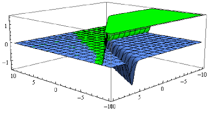
Figure 1: One line soliton $[1,0]$ solution $\tilde{u}(x,y,t=0)=u(x,y,t=0)+\epsilon$ (4.10) (blue) and squared absolute value of corresponding wave function $|\psi^{[1,0]}(i\mu_{10})|^{2}$ (green) (4.11) with parameters $a_{10}=-1,\epsilon=1,\lambda_{10}=1,\mu_{10}=4$.

Wave functions $\psi^{[1,0]}(i\mu_{10})$, $\psi^{[1,0]}(-i\lambda_{10})$ and $\psi^{[1,0]}(\lambda)$ due to formulas (3.16), (3.17) and (4.7)-(4.9) have the following forms:

$$\psi^{[1,0]}(i\mu_{10})=\frac{e^{F(i\mu_{10})}}{1+e^{\varphi_{1}+\phi_{0}}},\quad\psi^{[1,0]}(-i\lambda_{10})=\frac{e^{-F(i\lambda_{10})}}{1+e^{\varphi_{1}+\phi_{01}}};$$ (4.11)

$$\psi^{[1,0]}(\lambda)=e^{F(\lambda)}-\Big{(}\frac{i\lambda_{10}}{\lambda-i\lambda_{10}}+\frac{i\mu_{10}}{\lambda+i\mu_{10}}\Big{)}{\frac{2a_{10}e^{\varphi_{1}+F(\lambda)}}{1+e^{\varphi_{1}+\phi_{01}}}}.$$ (4.12)

Graphs of one line $[1,0]$ soliton (4.10) and the squared absolute value of wave function $\psi^{[1,0]}(i\mu_{10})$ (4.11) for certain values of parameters are presented in Fig.1. Graph of the squared absolute value of another wave function - $\psi^{[1,0]}(-i\lambda_{10})$ has the similar form but with localization along another one half of potential valley

Two line soliton $[2,0]$ solution in considered case of kernel $R_{0}$ (4.5) with parameters (3.12),(4)-(4.8) is given by the formula (3.18). It is remarkable that under the condition $q=p_{1}p_{2}$ (see (3.22)) which is equivalent to the relation:

$$(\lambda_{10}\mu_{10}+\lambda_{20}\mu_{20})(\lambda_{10}-\mu_{10})(\lambda_{20}-\mu_{20})=0,$$ (4.13)

i. e. to relation $\lambda_{10}\mu_{10}+\lambda_{20}\mu_{20}=0$ (due to $\lambda_{n0}\neq\mu_{n0}$, we do not consider in the present paper lumps!), the solution (3.18) radically simplifies and due to (3) takes the form:

$$u(\xi,\eta,t)=-\epsilon-\frac{\epsilon(\lambda_{10}-\mu_{10})^{2}}{2\lambda_{10}\mu_{10}}\frac{1}{\cosh^{2}{\frac{\varphi_{1}(\xi,\eta,t)+\phi_{01}}{2}}}-\frac{\epsilon(\lambda_{20}-\mu_{20})^{2}}{2\lambda_{20}\mu_{20}}\frac{1}{\cosh^{2}{\frac{\varphi_{2}(\xi,\eta,t)+\phi_{02}}{2}}}.$$ (4.14)

a) b) Figure 2: Two line soliton $[2,0]$ solution ${\tilde{u}(x,y,{t=0})=u(x,y,{t=0})+\epsilon}$ (4.14) (a) and squared absolute value of corresponding wave function $|\psi^{[2,0]}(i\mu_{10})|^{2}$ (green) (b), with parameters $a_{10}=1,\lambda_{10}=1,\mu_{10}=-3;a_{20}=-1,\lambda_{20}=4,\epsilon=-1$.

The corresponding wave functions $\chi^{[2,0]},\psi^{[2,0]}$ calculated in considered case of kernel $R_{0}$ (4.5) with parameters (4)-(4.8) by the formulas (2.27)-(2), under condition $p_{1}p_{2}=q$, i. e. under $\lambda_{10}\mu_{10}+\lambda_{20}\mu_{20}=0$, are given by the simple formulas (3.25)-(3). Graphs of two line $[2,0]$ soliton (4.14) and the squared absolute value of wave function - $\psi^{[2,0]}(i\mu_{10})$ (3.31) for certain values of parameters are presented in Fig.2 (the squared absolute values of other wave functions (3.32-3.34) have similar forms but with localization along another three possible halves of two potential valleys).

${\overline{\partial}}$-dressing in present paper is carried out for the fixed nonzero value of parameter $\epsilon$. Nevertheless one can correctly set $\epsilon=c_{k}\mu_{k0},(k=1,2)$ ($c_{k}$-arbitrary complex constant) and consider the limit $\epsilon\rightarrow 0$ in all derived formulas and obtain some interesting results also for the case of $\epsilon=0$. Limiting procedure $\epsilon=c_{k}\mu_{k0}\rightarrow 0,(k=1,2)$ can be correctly performed by the following settings in all required formulas: $\epsilon\rightarrow 0$ and $\mu_{k0}\rightarrow 0$ in cases when uncertainty is absent, but $\frac{\mu_{20}}{\mu_{10}}=-\frac{\lambda_{10}}{\lambda_{20}}\rightarrow\frac{c_{1}}{c_{2}}$ in accordance with the relations $\epsilon=c_{k}\mu_{k0}$ and $\mu_{10}\lambda_{10}+\mu_{20}\lambda_{20}=0$; the last relation is assumed to be valid in considered limit. The two line soliton solution (4.14) in the limit $\epsilon\rightarrow 0$ takes the form:

$$u=-\frac{c_{1}\lambda_{10}}{2\cosh^{2}{\frac{\varphi_{1}(\xi,\eta,t)+\phi_{01}}{2}}}-\frac{c_{2}\lambda_{20}}{2\cosh^{2}{\frac{\varphi_{2}(\xi,\eta,t)+\phi_{02}}{2}}},$$ (4.15)

where the phases $\varphi_{k}(\xi,\eta,t)$ and $\phi_{0k}$ due to (4.8), (4.9) have in considered limit the forms:

$$\varphi_{k}(\xi,\eta,t)=\lambda_{k0}\xi-c_{k}\eta-\kappa_{1}\lambda_{k0}^{3}t+\kappa_{2}c_{k}^{3}t,\quad\phi_{0k}=\ln(-a_{k0}).$$ (4.16)

One can check by direct substitution that NVN-II equation (1.1) with $\sigma=1$ satisfies by $u$ given by (4.15), it satisfies also by each item

$$u^{(k)}=-\frac{c_{k}\lambda_{k0}}{2\cosh^{2}{\frac{\varphi_{k}(\xi,\eta,t)+\phi_{0k}}{2}}},\quad(k=1,2)$$ (4.17)

of the sum (4.15). So in considered case the linear principle of superposition $u=u^{(1)}+u^{(2)}$ for such special solutions $u^{(1)},u^{(2)}$ (4.17) is valid.

4.2  $[0,1]$ and $[0,2]$ line solitons

To $[0,1]$, $[0,2]$ solitons the kernels of type $R_{0}$ (4.5) with values $L=0;\quad N=1,2$ (i. e. $a_{l0}=0,l=1,...,L;a^{\prime}_{n0}\neq 0,n=1,2$) in (4) are correspond. For nonsingular one line $[0,1]$ and two line $[0,2]$ soliton solutions of hyperbolic version of NVN equation parameters $\mu_{k},\lambda_{k},a_{k}$ in general formulas (3.9)-(3) of Section 3 must be identified due to (4) by the following way:

$$\mu_{k}=\overline{\lambda}_{k},\>\>a_{k}=\overline{a}_{k}:=a_{k0},\quad(k=1,2).$$ (4.18)

The parameters $p_{k}$, $(k=1,2)$, $q$ in (3.9)-(3) due to (4.18) are given by the expressions:

$$p_{k}=-a_{k0}\frac{\lambda_{kR}}{\lambda_{kI}}:=e^{\phi_{0k}}>0,\quad q=p_{1}p_{2}\cdot\Bigg{|}\frac{(\lambda_{1}-\lambda_{2})(\lambda_{1}+\bar{\lambda}_{2})}{(\lambda_{1}+\lambda_{2})(\lambda_{1}-\bar{\lambda}_{2})}\Bigg{|}^{2},$$ (4.19)

where the parameters $p_{k}:=e^{\phi_{0k}}>0$ are chosen as positive constants.

The real phases $\Delta F(\mu_{k},\lambda_{k})=F(\mu_{k})-F(\lambda_{k}):=\varphi_{k},(k=1,2)$ in (3.9)-(3) are given due to (2.4) in considered case by the expressions:

$$\varphi_{k}(\xi,\eta,t)=i\Big{[}(\overline{\lambda}_{k}-\lambda_{k})\xi-\epsilon\Big{(}\frac{1}{\overline{\lambda}_{k}}-\frac{1}{\lambda_{k}}\Big{)}\eta+\kappa_{1}(\overline{\lambda}_{k}^{3}-\lambda_{k}^{3})t-\kappa_{2}\epsilon^{3}\Big{(}\frac{1}{\overline{\lambda}_{k}^{3}}-\frac{1}{\lambda_{k}^{3}}\Big{)}t\Big{]}.$$ (4.20)

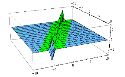
Figure 3: One line soliton $[0,1]$ solution $\tilde{u}(x,y,t=0)=u(x,y,t=0)+\epsilon$ (4.21) (blue) and squared absolute value of corresponding wave functions $|\psi^{[0,1]}(\overline{\lambda}_{1})|^{2}=|\psi^{[0,1]}(-\lambda_{1})|^{2}$ (green) (4.22) with parameters $a_{10}=-1,\lambda_{1R}=0.2,\lambda_{1I}=2,\epsilon=-1$.

One line soliton $[0,1]$ solution generated by simplest kernel $R_{0}$ of the type (4.5) with $L=0,N=1$ and parameters (4) due to (3.13) and (4.18)-(4.20) is nonsingular line soliton:

$$u=-\epsilon+\frac{2\epsilon\lambda_{1I}^{2}}{|\lambda_{1}|^{2}}\frac{1}{\cosh^{2}\frac{\varphi_{1}(\xi,\eta,t)+\phi_{01}}{2}}.$$ (4.21)

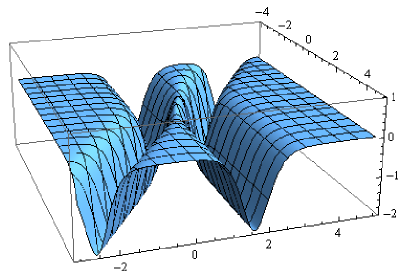
Figure 4: Two line soliton $[0,2]$ solution $\tilde{u}(x,y,t=0)=u(x,y,t=0)+\epsilon$ with parameters $a_{10}=-1,\lambda_{1R}=0.2,\lambda_{1I}=2;a_{20}=-1,\lambda_{2R}=0.1,\lambda_{2I}=1,\epsilon=-2$.

The corresponding wave functions $\psi^{[0,1]}(\mu_{1})=\chi^{[0,1]}(\mu_{1})e^{F(\mu_{1})}$, $\psi^{[0,1]}(-\lambda_{1})=\chi^{[0,1]}(-\lambda_{1})e^{F(-\lambda_{1})}$ and $\psi^{[0,1]}(\lambda)=\chi^{[0,1]}(\lambda)e^{F(\lambda)}$ of linear auxiliary problems (1.2),(1.3) and exact potential $u=\tilde{u}-\epsilon$ of one-dimensional perturbed telegraph equation (1.6) due to (3.16)-(3.17) and (4.18)-(4.20) have the forms:

$$\psi^{[0,1]}(\overline{\lambda}_{1})={\frac{e^{F(\overline{\lambda}_{1})}}{1+e^{\varphi_{1}+\phi_{01}}}},\quad\psi^{[0,1]}(-\lambda_{1})={\frac{e^{-F(\lambda_{1})}}{1+e^{\varphi_{1}+\phi_{01}}}};$$ (4.22)

$$\psi^{[0,1]}(\lambda)=e^{F(\lambda)}-\Big{(}\frac{\lambda_{1}}{\lambda-\lambda_{1}}+\frac{\overline{\lambda}_{1}}{\lambda+\overline{\lambda}_{1}}\Big{)}\frac{2ia_{10}e^{\varphi_{1}+F(\lambda)}}{1+e^{\varphi_{1}+\phi_{01}}}.$$ (4.23)

Graphs of one line $[0,1]$ soliton (4.21) and the squared absolute values of wave functions (4.22) for certain values of parameters are shown in Fig.3.

Two line soliton solution in considered case of kernel (4.5) with $L=0,N=2$ and parameters (4),(4.19) is given by the formula (3.18). It is interesting to note that the condition $q=p_{1}p_{2}$ in the considered case of kernel $R_{0}$ of the type (4.5) with $L=0,N=2$ and parameters (4),(4.18), (4.19) due to (3.24) takes the form $\lambda_{1}\mu_{1}+\lambda_{2}\mu_{2}=|\lambda_{1}|^{2}+|\lambda_{2}|^{2}=0$ and can not be satisfied for $\lambda_{k}\neq 0$, by this reason splitting of two line soliton solution (3.18)-(3.20) into the simple form (3) in the present case is impossible. Graph of two line $[0,2]$ soliton given by (3.18)-(3.20) for certain values of corresponding parameters is shown in Fig.4.

4.3  $[1,1]$ line soliton

To $[1,1]$ soliton corresponds the kernel of type $R_{0}$ (4.5) with values $L=1;\quad N=1$ (i. e. $a_{10}\neq 0,a^{\prime}_{10}\neq 0$) in (4). For nonsingular two line $[1,1]$ soliton solution of hyperbolic version of NVN equation parameters $\mu_{k},\lambda_{k},a_{k}$ in general formulas (3.9)-(3) of Section 3 must be identified due to (4) by the following way:

$$\mu_{1}=-\overline{\mu}_{1}:=i\mu_{10},\>\>\lambda_{1}=-\overline{\lambda}_{1}:=i\lambda_{10},\>\>a_{1}=-\overline{a}_{1}:=-ia_{10},$$

$$\mu_{2}=\mu^{\prime}_{1},\>\>\lambda_{2}=\lambda^{\prime}_{1}=\overline{\mu^{\prime}}_{1},\>\>a_{2}=a^{\prime}_{1}=\overline{a^{\prime}}_{1}:=a^{\prime}_{10},$$ (4.24)

$a_{2}$, $\lambda_{2}$, $\mu_{2}$ in formulas (3.18)-(3) due (4) must be identified with $a^{\prime}_{1}$, $\lambda^{\prime}_{1}$, $\mu^{\prime}_{1}$ in (4.5). The parameters $p_{k}$, $(k=1,2)$, $q$ in (3.9)-(3) due to (3.11) and (4) are given by expressions:

$$p_{1}=a_{10}\frac{\mu_{10}+\lambda_{10}}{\mu_{10}-\lambda_{10}}:=e^{\phi_{01}}>0,\quad p_{2}=-a_{20}\frac{\lambda_{2R}}{\lambda_{2I}}:=e^{\phi_{02}}>0.$$ (4.25)

Two line soliton $[1,1]$ solution in considered case with parameters (3.12), (4) is given by the formula (3.18). It is remarkable that under the condition $q=p_{1}p_{2}$ (see (3.22)) which is equivalent to the relation:

$$(-\lambda_{10}\mu_{10}+|\lambda_{2}|^{2})(i\lambda_{10}-i\mu_{10})(\lambda_{2}-\overline{\lambda}_{2})=0,$$ (4.26)

i. e. to relation $-\lambda_{10}\mu_{10}+|\lambda_{2}|^{2}=0$ (due to $\lambda_{n0}\neq\mu_{n0}$, we do not consider in the present paper lumps!), the solution (3) radically simplifies and due to (3) takes the form:

$$u(\xi,\eta,t)=-\epsilon-\frac{\epsilon(\lambda_{10}-\mu_{10})^{2}}{2\lambda_{10}\mu_{10}}\frac{1}{\cosh^{2}{\frac{\varphi_{1}(\xi,\eta,t)+\phi_{01}}{2}}}+\frac{2\epsilon\lambda^{2}_{2I}}{|\lambda_{2}|^{2}}\frac{1}{\cosh^{2}\frac{\varphi_{2}(\xi,\eta,t)+\phi_{02}}{2}},$$ (4.27)

where phases $\varphi_{1}(\xi,\eta,t)$, $\varphi_{2}(\xi,\eta,t)$ are given by the formulas (4.9),(4.20).

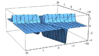
Figure 5: Two line soliton $[1,1]$ solution $\tilde{u}(x,y,t=0)=u(x,y,t=0)+\epsilon$ (4.27) with parameters $a_{10}=-0.1,\lambda_{10}=2,\epsilon=-2;a_{20}=-0.1,\lambda_{2R}=0.1,\lambda_{2I}=1$.

a b Figure 6: Nonbounded $|\psi^{[1,1]}(i\mu_{10})|^{2}$(a) and bounded $|\psi^{[1,1]}(\overline{\lambda}_{1})|^{2}=|\psi^{[1,1]}(-\lambda_{1})|^{2}$(b) squared absolute values of wave functions (green) corresponding to solution in the Fig.5.

The corresponding wave functions $\chi^{[1,1]},\psi^{[1,1]}$ calculated in considered case of kernel $R_{0}$ (4.5) with parameters (4),(4) and by the formulas (2.27)-(2), under condition $p_{1}p_{2}=q$, i. e. under $-\lambda_{10}\mu_{10}+|\lambda_{2}|^{2}=0$, are given by the simple formulas (3.25)-(3). Graphs of two line $[1,1]$ soliton (4.27) and squared absolute values of some wave functions given by (3.31)-(3.33) for certain values of parameters are shown in Fig.5-Fig.6 (graphs of $|\psi^{[1,1]}(i\mu_{10})|^{2}$ and $|\psi^{[1,1]}(-i\lambda_{10})|^{2}$ are similar to each other but with localization along two different halves of corresponding potential valley).

In all considered cases for NVN-II equation (hyperbolic version) multi line solitons are finite but corresponding wave functions can take infinite values in some areas of the plane $(x,y)$, (Fig.1, 2, 6a). Only in two considered cases, for soliton $[0,1]$ and soliton $[1,1]$ the squared absolute value of corresponding wave functions $|\psi^{[0,1]}(\overline{\lambda}_{1})|^{2}=|\psi^{[0,1]}(-\lambda_{1})|^{2}$ (Fig.3) and $|\psi^{[1,1]}(\overline{\lambda}_{1})|^{2}=|\psi^{[1,1]}(-\lambda_{1})|^{2}$ (Fig.6b) are finite.

We have to mention that exact potentials (of types [0,1] and [1,0]) of (1.6) with corresponding wave functions (4.11), (4.22) in the paper [22] have been calculated and used for the construction of exact solutions of two-dimensional generalized integrable sine-Gordon equation (2DGSG). In the present paper time evolution (2) is taken into account and corresponding multi line soliton solutions of NVN-II equation are calculated.

5 Exact multi line soliton solutions of NVN-I equation

For elliptic version of NVN equation (1.1), or NVN-I equation, with $\sigma^{2}=-1$ and complex space variables $\xi:=z=x+iy$, $\eta:=\bar{z}=x-iy$ an application of reality condition (2.24) to each term of the sum (3) for $R_{0}$ gives the following relation:

$$a_{k}\lambda_{k}\delta(\mu-\mu_{k})\delta(\lambda-\lambda_{k})+a_{k}\mu_{k}\delta(\mu+\lambda_{k})\delta(\lambda+\mu_{k})=$$

$$=\frac{\epsilon^{3}}{|\lambda|^{2}|\mu|^{2}\overline{\lambda}\overline{\mu}}\Big{[}\overline{a}_{k}\overline{\lambda}_{k}\delta\Big{(}-\frac{\epsilon}{\overline{\lambda}}-\mu_{k}\Big{)}\delta\Big{(}-\frac{\epsilon}{\overline{\mu}}-\lambda_{k}\Big{)}+\overline{a}_{k}\overline{\mu}_{k}\delta\Big{(}-\frac{\epsilon}{\overline{\lambda}}+\lambda_{k}\Big{)}\delta\Big{(}-\frac{\epsilon}{\overline{\mu}}+\mu_{k}\Big{)}\Big{]}=$$

$$=\frac{\epsilon\overline{a}_{k}}{\overline{\mu}_{k}}\delta\Big{(}\lambda+\frac{\epsilon}{\overline{\mu}_{k}}\Big{)}\delta\Big{(}\mu+\frac{\epsilon}{\overline{\lambda}_{k}}\Big{)}+\frac{\epsilon\overline{a}_{k}}{\overline{\lambda}_{k}}\delta\Big{(}\lambda-\frac{\epsilon}{\overline{\lambda}_{k}}\Big{)}\delta\Big{(}\mu-\frac{\epsilon}{\overline{\mu}_{k}}\Big{)}.$$ (5.1)

We should underline that in the present paper complex delta functions (with complex arguments) are used. The last equality in (5.1) by the well known property of complex delta functions $\delta(\varphi(z))=\sum\limits_{k}\delta(z-z_{k})/|\varphi^{\prime}(z_{k})|^{2}$ is obtained; $z_{k}$ in last formula are simple roots of equation $\varphi(z_{k})=0$.

From (5.1) two possibilities are follow:

$$1.\quad a_{k}\lambda_{k}=\frac{\epsilon\overline{a}_{k}}{\overline{\mu}_{k}},\>\>\lambda_{k}=-\frac{\epsilon}{\overline{\mu}_{k}},\>\>\mu_{k}=-\frac{\epsilon}{\overline{\lambda}_{k}};\quad 2.\quad a_{k}\lambda_{k}=\frac{\epsilon\overline{a}_{k}}{\overline{\lambda}_{k}},\>\>\lambda_{k}=\frac{\epsilon}{\overline{\lambda}_{k}},\>\>\mu_{k}=\frac{\epsilon}{\overline{\mu}_{k}}.$$ (5.2)

For the first case in (5.2) taking into account the reality of $\epsilon$ one obtains

$$a_{k}=-\overline{a}_{k}:=ia_{k0},\>\>\epsilon=-\mu_{k}\overline{\lambda}_{k}=-\overline{\mu}_{k}\lambda_{k};\quad\arg(\mu_{k})=\arg(\lambda_{k})+m\pi,$$ (5.3)

i. e. pure imaginary amplitudes $a_{k}$ ($a_{k0}=\overline{a}_{k0}$) and the relation between arguments of discrete spectral points $\mu_{k}$ and $\lambda_{k}$ with $m$ arbitrary integer. From the second possibility in (5.2) for satisfying the reality condition (2.24) the following relations

$$a_{k}=\overline{a}_{k}:=a^{\prime}_{k0},\quad\epsilon=|\mu^{\prime}_{k}|^{2}=|\lambda^{\prime}_{k}|^{2};\>\>\arg(\mu^{\prime}_{k})=\arg(\lambda^{\prime}_{k})+\delta_{k}$$ (5.4)

with real amplitudes $a_{k}=\overline{a}_{k}:=a^{\prime}_{k0}$ and arbitrary constants $\delta_{k}$ are follow.

So the kernel (2.26), (3) satisfying to potentiality (2.25) and reality (2.23) conditions in considered two cases (4.2) due to (5.2)-(5.4) can be chosen in the following form

$$R_{0}(\mu,\overline{\mu},\lambda,\overline{\lambda})=\pi\sum\limits_{k=1}^{2(L+N)}A_{k}\delta(\mu-M_{k})\delta(\lambda-\Lambda_{k})$$ (5.5)

of $L$ pairs of the type $i\pi\big{(}a_{l0}\lambda_{l}\delta(\mu-\mu_{l})\delta(\lambda-\lambda_{l})+a_{l0}\mu_{l}\delta(\mu+\lambda_{l})\delta(\lambda+\mu_{l})\big{)}$  (here $\epsilon=-\mu_{l}\overline{\lambda}_{l}=-\overline{\mu}_{l}\lambda_{l},\quad(l=1,..,L)$); and $N$ pairs of the type $\pi\big{(}a^{\prime}_{n0}\lambda^{\prime}_{n}\delta(\mu-\mu^{\prime}_{n})\delta(\lambda-\lambda^{\prime}_{n})+a^{\prime}_{n0}\mu_{n}\delta(\mu+\lambda^{\prime}_{n})\delta(\lambda+\mu^{\prime}_{n})\big{)}$  (here $\epsilon=|\lambda^{\prime}_{n}|^{2}=|\mu^{\prime}_{n}|^{2},\quad(n=1,..,N)$) of corresponding items. Here in (5.5) for application of general determinant formulas (7.19), (2.36) and (7.17) due to (5.2)-(5.4) the following sets of amplitudes $A_{k}$ and spectral parameters $M_{k}$, $\Lambda_{k}$

$$(A_{1},..,A_{2(L+N)})=$$

$$=(ia_{10}\lambda_{1},..,ia_{L0}\lambda_{L};ia_{10}\mu_{1},..,ia_{L0}\mu_{L};a^{\prime}_{10}\lambda^{\prime}_{1},..,a^{\prime}_{N0}\lambda^{\prime}_{N};a^{\prime}_{10}\mu^{\prime}_{1},..,a^{\prime}_{N0}\mu^{\prime}_{N}),$$

$$(M_{1},..,M_{2(L+N)})=(\mu_{1},..,\mu_{L};-\lambda_{1},..,-\lambda_{L};\mu^{\prime}_{1},..,\mu^{\prime}_{N};-\lambda^{\prime}_{1},..,-\lambda^{\prime}_{N}),$$

$$(\Lambda_{1},..,\Lambda_{2(L+N)})=(\lambda_{1},..,\lambda_{N};-\mu_{1},..,-\mu_{N};\lambda^{\prime}_{1},..,\lambda^{\prime}_{N};-\mu^{\prime}_{1},..,-\mu^{\prime}_{N})$$ (5.6)

are introduced.

General determinant formula (2.36) with matrix $A$ from (7.19) with corresponding parameters (5) of kernels $R_{0}$ (5.5) of $\overline{\partial}$-problem (2.1) gives exact multi line soliton solutions $u(z,\overline{z},t)$ with constant asymptotic value $-\epsilon$ at infinity of elliptic version of NVN equation. Simultaneously an application of general scheme of $\overline{\partial}$-dressing method gives exact potentials $u$ and corresponding wave functions $\chi^{[L,N]}(M_{l})$, $\psi^{[L,N]}(M_{l})=\chi^{[L,N]}(M_{l})e^{F(M_{l})}$ at discrete spectral parameters $M_{l}$ and $\chi^{[L,N]}(\lambda)$, $\psi^{[L,N]}(\lambda)=\chi^{[L,N]}(\lambda)e^{F(\lambda)}$ at continuous spectral parameter $\lambda$ of linear auxiliary problems (1.2),(1.3) and two-dimensional stationary Schrödinger equation (1.7). Here and below the symbols $\chi^{[L,N]},\psi^{[L,N]}$ denote the wave functions of multi line soliton exact solution corresponding to the general kernel (5.5) with $L+N$ pairs of items.

The rest of the section is devoted to the presentation for considered two cases (5.2) of the explicit forms of some one line of types $[1,0],[0,1]$ and two line soliton solutions of types $[2,0],[0,2],[1,1]$ of elliptic version of NVN equation and exact potentials with corresponding wave functions of two-dimensional stationary Schrödinger equation (1.7).

5.1  $[1,0],[2,0]$ line solitons

To $[1,0]$, $[2,0]$ line solitons the kernels of type $R_{0}$ (5.5) with values $L=1,2;\quad N=0$ (i. e. $a_{l0}\neq 0,l=1,2;a^{\prime}_{n0}=0,n=1,...,N$) in (5) are correspond.

For nonsingular one line $[1,0]$ and two line $[2,0]$ soliton solutions of elliptic version of NVN equation parameters $\mu_{k},\lambda_{k},a_{k}$ in general formulas (3.9)-(3) of Section 3 must be identified due to (5) by the following way:

$$a_{k}=-\overline{a}_{k}:=ia_{k0},\quad\mu_{k}=-{\frac{\epsilon}{\overline{\lambda}_{k}}}\quad(k=1,2),$$ (5.7)

and real parameters $p_{k}$ (3.11)

$$p_{k}=a_{k0}\frac{\lambda_{k}+\mu_{k}}{\lambda_{k}-\mu_{k}}=e^{\phi_{0k}}>0,\quad(k=1,2)$$ (5.8)

as positive constants must be chosen. The real phases $\Delta F(\mu_{k},\lambda_{k})=F(\mu_{k})-F(\lambda_{k}):=\varphi_{k},(k=1,2)$ in (3.9)-(3) are given in considered case by the expressions:

$$\varphi_{k}(z,\bar{z},t)=i\big{[}(\mu_{k}-\lambda_{k})z-(\overline{\mu}_{k}-\overline{\lambda}_{k})\overline{z}+\kappa(\mu^{3}_{k}-\lambda_{k}^{3})t-\overline{\kappa}(\overline{\mu}_{k}^{3}-\overline{\lambda}_{k}^{3})t\big{]}.$$ (5.9)

One line soliton $[1,0]$ solution corresponding to simplest kernel $R_{0}$ of the type (5.5) with parameters (5) due to (5.7)-(5.9) is nonsingular line soliton:

$$u=-\epsilon-\frac{\epsilon(\lambda_{1}-\mu_{1})^{2}}{2\lambda_{1}\mu_{1}}\frac{1}{\cosh^{2}\frac{\varphi_{1}+\phi_{01}}{2}}=-\epsilon+\frac{|\lambda_{1}-\mu_{1}|^{2}}{2}\frac{1}{\cosh^{2}\frac{\varphi_{1}+\phi_{01}}{2}};\quad\epsilon=-\lambda_{1}\bar{\mu}_{1}.$$ (5.10)

a b

c Figure 7: Potential $V_{Shr}$ (5.13) (blue) with the energy level $E$ (yellow) and corresponding squared absolute values of wave functions $|\psi^{[1,0]}(\mu_{1})|^{2}=|\psi^{[1,0]}(-\lambda_{1})|^{2}$ (5.11) (green) with parameters: a) $a_{10}=-0.1,\lambda_{1}=e^{i\frac{\pi}{6}},\mu_{1}=4e^{i\frac{7\pi}{6}},E=-2\epsilon=-8$; b) $a_{10}=-0.1,\lambda_{1}=e^{i\frac{\pi}{6}},\mu_{1}=4e^{i\frac{\pi}{6}},E=-2\epsilon=8$; c) $a_{10}=0.1,\lambda_{1}=e^{i\frac{\pi}{6}},\mu_{1}=0,E=-2\epsilon=0$.

The corresponding wave functions $\psi^{[1,0]}(\mu_{1})=\chi^{[1,0]}(\mu_{1})e^{F(\mu_{1})}$, $\psi^{[1,0]}(-\lambda_{1})=\chi^{[1,0]}(-\lambda_{1})e^{F(-\lambda_{1})}$ and $\psi^{[1,0]}(\lambda)=\chi(\lambda)e^{F(\lambda)}$ of linear auxiliary problems (1.2),(1.3) and exact potential $V_{Shr}$ of 2D stationary Schrödinger equation (1.7) with energy level $E:=-2\epsilon$ due to (2), (3.14)-(3.17) have the forms:

$$\psi(\mu_{1})=\frac{e^{F(\mu_{1})}}{1+e^{\varphi_{1}+\phi_{01}}},\quad\psi(-\lambda_{1})=\frac{e^{-F(\lambda_{1})}}{1+e^{\varphi_{1}+\phi_{01}}},$$ (5.11)

$$\psi(\lambda)=e^{F(\lambda)}+\Big{(}\frac{\lambda_{1}}{\lambda-\lambda_{1}}+\frac{\mu_{1}}{\lambda+\mu_{1}}\Big{)}\frac{2a_{10}e^{\varphi_{1}+F(\lambda)}}{1+e^{\varphi_{1}+\phi_{01}}};$$ (5.12)

$$V_{Schr}=-\frac{E(\lambda_{1}-\mu_{1})^{2}}{\lambda_{1}\mu_{1}}\frac{1}{\cosh^{2}\frac{\varphi_{1}+\phi_{01}}{2}}=-\frac{|\lambda_{1}-\mu_{1}|^{2}}{\cosh^{2}\frac{\varphi_{1}+\phi_{01}}{2}};\quad E=-2\epsilon=2\lambda_{1}\bar{\mu}_{1}.$$ (5.13)

a b

c Figure 8: Potential $V_{Shr}$ corresponding two line soliton $[2,0]$ solution (5) (blue) with the energy level $E$ (yellow) with parameters: a) $a_{10}=-1,\lambda_{1}=e^{i\frac{\pi}{8}},\mu_{1}=1.05e^{i\frac{9\pi}{8}};a_{20}=-1,\tau=1,E=-2\epsilon=-2.1$; b) $a_{10}=-0.1,\lambda_{1}=e^{i\frac{\pi}{6}},\mu_{1}=4e^{i\frac{\pi}{6}};a_{20}=-0.1,\tau=1,E=-2\epsilon=8$; c) $a_{10}=0.1,\lambda_{1}=e^{i\frac{\pi}{6}},\mu_{1}=0;a_{20}=0.1,\tau=1,E=-2\epsilon=0$.

Graphs of Schrödinger potentials (5.13) (connected with one line $[1,0]$ solitons $V_{Schr}=-2\tilde{u}$ (5.10)) and squared absolute values of wave functions (5.11) for stationary states with energies $E<0$, $E>0$ and  $E=0$ (equation (1.7) for particle with mass $m=1$) for certain values of corresponding parameters are shown in Fig.7. One can prove that two wave functions (5.11) for all signs of energy correspond to stationary states of a particle with opposite to each other conserved projections (on direction of valley) of momentum. In all above mentioned stationary states with wave functions (5.11) particle is bounded in transverse direction to potential valley and moves freely along the direction of potential valley.

Two line soliton $[2,0]$ solution in considered case of kernel $R_{0}$ of the type (5.5) with parameters (5) is given by the formula (3.18), it is remarkable that under the condition $q=p_{1}p_{2}$ this solution radically simplifies. Indeed, due to (3.24) condition $q=p_{1}p_{2}$ is satisfied if $\lambda_{1}\mu_{1}+\lambda_{2}\mu_{2}=0$ and in this case two line soliton solution (3.18) takes the form (3):

$$u(z,\bar{z},t)=-\epsilon-\frac{\epsilon(\lambda_{1}-\mu_{1})^{2}}{2\lambda_{1}\mu_{1}}\frac{1}{\cosh^{2}{\frac{\varphi_{1}(z,\bar{z},t)+\phi_{01}}{2}}}-\frac{\epsilon(\lambda_{2}-\mu_{2})^{2}}{2\lambda_{2}\mu_{2}}\frac{1}{\cosh^{2}{\frac{\varphi_{2}(z,\bar{z},t)+\phi_{02}}{2}}}=$$

$$=-\epsilon+\frac{|\lambda_{1}-\mu_{1}|^{2}}{2}\frac{1}{\cosh^{2}{\frac{\varphi_{1}(z,\bar{z},t)+\phi_{01}}{2}}}+\frac{|\lambda_{2}-\mu_{2}|^{2}}{2}\frac{1}{\cosh^{2}{\frac{\varphi_{2}(z,\bar{z},t)+\phi_{02}}{2}}}.$$ (5.14)

From the relation $\lambda_{1}\mu_{1}+\lambda_{2}\mu_{2}=0$ taking into account the first condition (5.2) ($\lambda_{1}\overline{\mu}_{1}=\overline{\lambda}_{1}\mu_{1}=\lambda_{2}\overline{\mu}_{2}=\overline{\lambda}_{2}\mu_{2}=-\epsilon$) follows $\overline{\mu}_{2}/\overline{\mu}_{1}=-\mu_{2}/\mu_{1}=\lambda_{1}/\lambda_{2}$ and from the last relation one obtains

$$\mu_{2}=i\tau{\mu}_{1},\quad\lambda_{2}=i\tau^{-1}{\lambda}_{1},\quad\tau=\bar{\tau}$$ (5.15)

with arbitrary real constant $\tau$.

Wave functions corresponding to two line soliton $[2,0]$ solution (5) in considered case of kernel $R_{0}$ of the type (5.5) with parameters (5) and (5.7)-(5.9), under condition $p_{1}p_{2}=q$, are given by very simple expressions (3.25)-(3).

a b

c Figure 9: Squared absolute values of wave functions $|\psi^{[2,0]}(\mu_{1})|^{2}=|\psi^{[2,0]}(-\lambda_{1})|^{2}$ (green) corresponding to different values of energy $E$ in the Fig.8(a,b,c).

Graphs of Schrödinger potentials (connected with two line $[2,0]$ soliton $V_{Schr}=-2\tilde{u}$ solutions (5)) and squared absolute values $|\psi^{[2,0]}(\mu_{1})|^{2}=|\psi^{[2,0]}(-\lambda_{1})|^{2}$ of some wave functions from (3.31)-(3.34) for certain values of parameters are shown in Fig.8 and Fig.9 (graphs of $|\psi^{[2,0]}(\mu_{2})|^{2}=|\psi^{[2,0]}(-\lambda_{2})|^{2}$ are similar to graphs of $|\psi^{[2,0]}(\mu_{1})|^{2}=|\psi^{[2,0]}(-\lambda_{1})|^{2}$ but with localization along another soliton valley).

Calculated via ${\overline{\partial}}$-dressing method wave functions (3.31)-(3.34) at discrete values of spectral parameters correspond to possible physical basis states of particle localized in the field of two potential valleys. ${\overline{\partial}}$-dressing in present paper is carried out for the fixed nonzero value of parameter $\epsilon$ or, in context of present section, for nonzero energy $E\neq 0$. Nevertheless one can correctly consider the limit $\epsilon\rightarrow 0$ in all derived formulas and obtain some interesting results also for the case of zero energy $E=-2\epsilon=0$. Limiting procedure $E=-2\epsilon=\mu_{k}\bar{\lambda}_{k}+\bar{\mu}_{k}\lambda_{k}\rightarrow 0,(k=1,2)$ can be correctly performed by the following settings in all required formulas: $\epsilon\rightarrow 0$ and $\mu_{k}\rightarrow 0$ in cases when uncertainty is absent, but ${\frac{\epsilon}{\mu_{k}}}\rightarrow-\bar{\lambda}_{k}$ in accordance with the relation $\epsilon=-\mu_{k}\bar{\lambda}_{k}$; in addition the formula $\lambda_{2}=i\tau^{-1}\lambda_{1}$ (5.15) (followed from the relations $\bar{\mu}_{k}\lambda_{k}=\mu_{k}\bar{\lambda}_{k}$ and $\mu_{1}\lambda_{1}+\mu_{2}\lambda_{2}=0$) with arbitrary real constant $\tau$ is assumed to be valid. The two line soliton solution due to (5) in considered limit has the form:

$$u=\frac{|\lambda_{1}|^{2}}{2\cosh^{2}{\frac{\varphi_{1}(z,\bar{z})+\phi_{01}}{2}}}+\frac{|\lambda_{2}|^{2}}{2\cosh^{2}{\frac{\varphi_{2}(z,\bar{z})+\phi_{02}}{2}}},$$ (5.16)

the phases $\varphi_{k}(z,\bar{z})$ and $\phi_{0k}$ due to (2.4),(5.9),(5.8) have in considered limit the forms:

$$\varphi_{k}(z,\bar{z},t)=-i\big{(}\lambda_{k}z-\overline{\lambda}_{k}\overline{z}+\kappa\lambda_{k}^{3}t-\overline{\kappa}\overline{\lambda}_{k}^{3}t\big{)},\quad\phi_{0k}=\ln{a_{k0}}.$$ (5.17)

One can check by direct substitution that NVN-I equation (1.1) with $\sigma=i$ satisfies by $u=\tilde{u}=-V_{Schr}/2$ given by (5.16), but it also satisfies by each item

$$u^{(k)}={\frac{|\lambda_{k}|^{2}}{2\cosh^{2}{\frac{\varphi_{k}(z,\bar{z})+\phi_{0k}}{2}}}},\quad(k=1,2)$$ (5.18)

of the sum (5.16). Thus, in considered case the linear principle of superposition $u=u^{(1)}+u^{(2)}$ for such special solutions $u^{(1)},u^{(2)}$ (5.18) is valid. One can show using (5.15),(5.17) that line solitons $u^{(1)}$ and $u^{(2)}$ are propagate in the plane $(x,y)$ in perpendicular to each other directions. Schrödinger potentials $V_{Schr}$ (of the types [1,0] and [2,0]) with corresponding squared absolute value wave functions of zero energy limit $E=0$ are also pictured by graphs of Fig.7, Fig.8 and Fig.9.

5.2 $[0,1],[0,2]$ line solitons

The kernels of type $R_{0}$ (5.5) with values $L=0;\quad N=1,2$ (i. e. $a_{l0}=0,l=1,..,L;a^{\prime}_{n0}\neq 0,n=1,2$) in (5) correspond to $[0,1]$, $[0,2]$ line solitons. For nonsingular one line $[0,1]$ and two line $[0,2]$ soliton solutions of elliptic version of NVN equation parameters $a_{k},\mu_{k},\lambda_{k}$ in general formulas (3.9)-(3) of Section 3 must be identified due to (5) by the following way:

$$a_{k}=\overline{a}_{k}:=a_{k0},\quad\epsilon=|\mu_{k}|^{2}=|\lambda_{k}|^{2},\quad(k=1,2).$$ (5.19)

Real parameters $p_{k}$ due to (3.11), (5) and (5.19)

$$p_{k}=ia_{k0}\frac{\mu_{k}+\lambda_{k}}{\mu_{k}-\lambda_{k}}=a_{k0}\cot\frac{\delta_{k}}{2}:=e^{\phi_{0k}}>0,\quad\mu_{k}:=\lambda_{k}e^{i\delta_{k}},\quad(k=1,2)$$ (5.20)

appear as positive constants. The real phases $\Delta F(\mu_{k},\lambda_{k})=F(\mu_{k})-F(\lambda_{k}):=\varphi_{k},(k=1,2)$ are given in considered case by the expressions:

$$\varphi_{k}(z,\bar{z},t)=i[(\mu_{k}-\lambda_{k})z-(\overline{\mu}_{k}-\overline{\lambda}_{k})\overline{z}+\kappa(\mu_{k}^{3}-\lambda_{k}^{3})t-\overline{\kappa}(\overline{\mu}_{k}^{3}-\overline{\lambda}_{k}^{3})t].$$ (5.21)

One line soliton $[0,1]$ solution corresponding to simplest kernel $R_{0}$ of the type (5.5) with parameters (5) due to (3.13) and (5.19)-(5.20) and (5.21) is nonsingular line soliton:

$$u=-\epsilon+\frac{|\lambda_{1}-\mu_{1}|^{2}}{2}\frac{1}{\cosh^{2}\frac{\varphi_{1}+\phi_{01}}{2}}=-\epsilon+\frac{2\epsilon\sin^{2}\frac{\delta_{1}}{2}}{\cosh^{2}\frac{\varphi_{1}+\phi_{01}}{2}}.$$ (5.22)

The corresponding wave functions $\psi^{[0,1]}(\mu_{1})=\chi^{[0,1]}(\mu_{1})e^{F(\mu_{1})}$, $\psi^{[0,1]}(-\lambda_{1})=\chi^{[0,1]}(-\lambda_{1})e^{F(-\lambda_{1})}$ and $\psi^{[0,1]}(\lambda)=\chi^{[0,1]}(\lambda)e^{F(\lambda)}$ of linear auxiliary problems (1.2),(1.3) and exact potential $V_{Shr}$ of 2D stationary Schrödinger equation (1.7) with energy level $E:=-2\epsilon$ have forms:

$$\psi(\mu_{1})=\frac{e^{F(\mu_{1})}}{1+e^{\varphi_{1}+\phi_{01}}},\quad\psi(-\lambda_{1})=\frac{e^{-F(\lambda_{1})}}{1+e^{\varphi_{1}+\phi_{01}}},$$ (5.23)

$$\psi(\lambda)=e^{F(\lambda)}-\Big{(}\frac{\lambda_{1}}{\lambda-\lambda_{1}}+\frac{\mu_{1}}{\lambda+\mu_{1}}\Big{)}\frac{2ia_{10}e^{\varphi_{1}+F(\lambda)}}{1+e^{\varphi_{1}+\phi_{01}}};$$ (5.24)

$$V_{Schr}=-\frac{|\lambda_{1}-\mu_{1}|^{2}}{\cosh^{2}\frac{\varphi_{1}+\phi_{01}}{2}}=-\frac{4\epsilon\sin^{2}(\frac{\delta_{1}}{2})}{\cosh^{2}\frac{\varphi_{1}+\phi_{01}}{2}};E=-2\epsilon=-2|\lambda_{1}|^{2}=-2|\mu_{1}|^{2}.$$ (5.25)

a b

Figure 10: Potential $V_{Shr}$ (5.22) (blue) with the energy level $E$ (yellow) and corresponding squared absolute value of wave function $|\psi^{[0,1]}(\mu_{1})|^{2}$ (5.23) (green) with parameters: a) $a_{10}=-1,\lambda=2-i,\delta=\frac{10\pi}{9},E=-2\epsilon=-10$; b) $a_{10}=-1,\lambda=2-i,\delta=\frac{\pi}{3},E=-2\epsilon=-10$.

Graphs of Schrödinger potential $V_{Schr}$ (5.25) (connected with one line $[0,1]$ soliton $V_{Schr}=-2\tilde{u}$ solution (5.22)) and the squared absolute value of wave function $\psi^{[0,1]}(\mu_{1})$ from (5.23) for certain values of parameters are shown in Fig.10: a) $(V_{Shr})_{min}<E<0$, b) $(V_{Shr})_{min}=E<0$ (the squared absolute value $|\psi^{[0,1]}(-\lambda_{1})|^{2}$ has the similar form but with localization along another one half of potential valley).

Two line soliton $[0,2]$ solution in considered case of kernel kernel $R_{0}$ of the type (5.5) with parameters (5) and (5.19),(5.20) and (5.21) is given by the formula (3.18). It is remarkable that under the condition $q=p_{1}p_{2}$ this solution radically simplifies. Indeed, due to (3.24) condition $q=p_{1}p_{2}$ is satisfied if $\lambda_{1}\mu_{1}+\lambda_{2}\mu_{2}=0$, in this case two line soliton solution (3.18) takes the form (3):

$$u(z,\bar{z},t)=-\epsilon+{\frac{|\lambda_{1}-\mu_{1}|^{2}}{2}}\frac{1}{\cosh^{2}{\frac{\varphi_{1}(z,\bar{z},t)+\phi_{01}}{2}}}+\frac{|\lambda_{1}-\mu_{1}|^{2}}{2}\frac{1}{\cosh^{2}{\frac{\varphi_{2}(z,\bar{z},t),+\phi_{02}}{2}}}=$$

$$=-\epsilon+\frac{2\epsilon\sin^{2}{\frac{\delta_{1}}{2}}}{\cosh^{2}{\frac{\varphi_{1}(z,\bar{z},t)+\phi_{01}}{2}}}+\frac{2\epsilon\sin^{2}{\frac{\delta_{2}}{2}}}{\cosh^{2}{\frac{\varphi_{2}(z,\bar{z},t)+\phi_{02}}{2}}},\quad\mu_{k}=\lambda_{k}e^{i\delta_{k}},\epsilon=|\lambda_{k}|^{2}=|\mu_{k}|^{2}.$$ (5.26)

a b

Figure 11: Potential $V_{Shr}$ corresponding two line soliton $[0,2]$ solution (5)(blue) with the energy level $E$(yellow) with parameters: (a) $a_{10}=-1,\lambda_{1}=2-i,\delta_{1}=\frac{10\pi}{9};a_{20}=1,\delta_{2}=\frac{3\pi}{10},E=-2\epsilon=-10$; (b) $a_{10}=1,\lambda_{1}=2-i,\delta_{1}=\frac{\pi}{3};a_{20}=1,\delta_{2}=\frac{3\pi}{5},E=-2\epsilon=-10$.

The corresponding to two line soliton solution (5) wave functions in considered case of kernel $R_{0}$ of the type (5.5) with parameters (5) and (5.19),(5.20) and (5.21), under condition $p_{1}p_{2}=q$, are given by very simple expressions (3.25)-(3).

a b

Figure 12: Squared absolute value of wave function $|\psi^{[0,2]}(\mu_{1})|^{2}$ (green) for the different types of crossings of potentials valleys by energy planes in the Fig.11 (a,b).

Graphs of Schrödinger potentials (connected with two line $[0,2]$ solitons $V_{Schr}=-2\tilde{u}$ (5)) and squared absolute value $|\psi^{[0,2]}(\mu_{1})|^{2}$ of one wave function from four linear independent partners (3.31)-(3.34) for certain values of parameters are shown in Fig.11 and Fig.12 (the squared absolute values of other wave functions have the similar forms but with localization along another three possible halves of two potential valleys). In all considered in the present section cases of one line [0,1] and two line [0,2] solitons $u=\tilde{u}-\epsilon$ and Schrödinger potentials $V_{Schr}=-2\tilde{u}$ corresponding wave functions (Fig.10, Fig.12) are not bounded.

5.3  $[1,1]$ line soliton

The kernel of type $R_{0}$ (5.5) with values $L=1;\quad N=1$ (i. e. $a_{10}=1;a^{\prime}_{10}=1$) in (5) correspond to $[1,1]$ line soliton. For this soliton solution parameters $a_{k},\mu_{k},\lambda_{k}$ in general formulas (3.9)-(3) of Section 3 must be identified due to (5) by the following way:

$$a_{1}=-\overline{a}_{1}:=ia_{10},\quad\epsilon=-\mu_{1}\overline{\lambda}_{1}$$

$$a_{2}=a^{\prime}_{1}=\overline{a}^{\prime}_{1}:=a^{\prime}_{10},\>\mu_{2}=\mu^{\prime}_{1},\>\lambda_{2}=\lambda^{\prime}_{1},\quad\epsilon=|\mu^{\prime}_{1}|^{2}=|\lambda^{\prime}_{1}|^{2}.$$ (5.27)

$a_{2}$, $\lambda_{2}$, $\mu_{2}$ in formulas (3.18)-(3) due (5) must be identified with $a^{\prime}_{1}$, $\lambda^{\prime}_{1}$, $\mu^{\prime}_{1}$ in (5.5). Real parameters $p_{1}$, $p_{2}$ due to (3.11), (5) and (5)

$$p_{1}=-a_{10}\frac{\mu_{1}+\lambda_{1}}{\mu_{1}-\lambda_{1}}:=e^{\phi_{01}}>0,\quad p_{2}=ia_{20}\frac{\mu_{2}+\lambda_{2}}{\mu_{2}-\lambda_{2}}=a_{20}\cot\frac{\delta_{2}}{2}:=e^{\phi_{02}}>0,$$ (5.28)

appear as positive constants.

Two line soliton $[1,1]$ solution in considered case of kernel kernel $R_{0}$ of the type (5.5) with parameters (3.12) and (5),(5.28) is given by the formula (3.18). It is remarkable that under the condition $q=p_{1}p_{2}$ this solution radically simplifies. Indeed, due to (3.24) condition $q=p_{1}p_{2}$ is satisfied if $\lambda_{1}\mu_{1}+\lambda_{2}\mu_{2}=0$, in this case two line soliton solution (3.18) takes the form (3:

$$u(z,\bar{z},t)=-\epsilon+\frac{|\lambda_{1}-\mu_{1}|^{2}}{2}\frac{1}{\cosh^{2}{\frac{\varphi_{1}(z,\bar{z},t)+\phi_{01}}{2}}}+\frac{|\lambda_{2}-\mu_{2}|^{2}}{2}\frac{1}{\cosh^{2}{\frac{\varphi_{2}(z,\bar{z},t)+\phi_{02}}{2}}}$$ (5.29)

where $|\lambda_{2}|^{2}=|\mu_{2}|^{2}=-\mu_{1}\overline{\lambda}_{1}=-\overline{\mu}_{1}\lambda_{1}=\epsilon$ and the phases $\varphi_{1}$, $\varphi_{2}$ are given by formulas (5.9),(5.21). Graphs of Schrödinger potentials (connected with two line $[1,1]$ solitons $V_{Schr}=-2\tilde{u}$ (5.29)) and squared absolute values of some wave functions from (3.31)-(3.34) for certain values of parameters are shown in Fig.13 and Fig.14 (graphs of $|\psi^{[1,1]}(-\lambda_{2})|^{2}$ and $|\psi^{[1,1]}(\mu_{2})|^{2}$ are similar to each other but with localization along two different halves of corresponding potential valley).

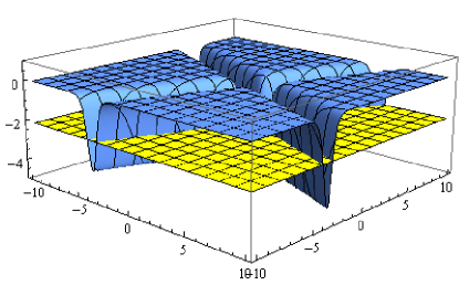
Figure 13: Potential $V_{Shr}$ corresponding two line soliton $[1,1]$ solution (3.18)(blue) and energy level E (yellow) with parameters $a_{1}=-1,\lambda_{1}=1e^{\frac{\pi}{8}},\mu_{1}=1.05e^{\frac{9\pi}{8}};a_{2}=-1,\lambda_{2}=1.0247e^{\frac{\pi}{2}},\mu_{2}=1.0247e^{\frac{7\pi}{4}},E=-2\epsilon=-2.1$.

a b

Figure 14: Bounded $|\psi^{[1,1]}(\mu_{1})|^{2}=|\psi^{[1,1]}(-\lambda_{1})|^{2}$ (a) and nonbounded $|\psi^{[1,1]}(\mu_{2})|^{2}$ (b) squared absolute values of wave functions (green) given by (3.31)-(3.33) corresponding to potential and energy in the Fig.13.

In considered in present section case of two line [1,1] soliton $u=\tilde{u}-\epsilon$ (5.29) with corresponding Schrödinger potential $V_{Schr}=-2\tilde{u}$ squared absolute values of wave functions $|\psi^{[1,1]}(\mu_{1})|^{2}=|\psi^{[1,1]}(-\lambda_{1})|^{2}$ are bounded (Fig.14a), but the squared absolute values of other basis wave functions $|\psi^{[1,1]}(\mu_{2})|^{2}$ and $|\psi^{[1,1]}(-\lambda_{2})|^{2}$ are not bounded (Fig.14b).

In conclusion of Section 5 let us mention that all constructed in subsection 5.1 solitons and corresponding wave functions are finite and have appropriate physical interpretation. For example, the wave function (5.12) of continuous spectral parameter $\lambda$ for discrete values of this parameter $\lambda=\mu_{1}$ or $\lambda=-\lambda_{1}$ coincides with wave functions (5.11); for positive values of energy $E=-2\epsilon>0$ and $\lambda\neq\mu_{1},\lambda\neq-\lambda_{1}$, under condition $|\lambda|^{2}=-\epsilon=E/2>0$, the wave function (5.12) corresponds to stationary states of nonlocalized on the plane $(x,y)$ particle which do not reflects from the constructed potential (5.13). In considered in subsections 5.2 and 5.3 cases multi line solitons are finite but corresponding wave functions can take infinite values in some areas of the plane $(x,y)$, (Fig.10, 12, 14b); only for two line soliton $[1,1]$ squared absolute values of wave functions $|\psi^{[1,1]}(\mu_{1})|^{2}=|\psi^{[1,1]}(-\lambda_{1})|^{2}$ (Fig.14a) are finite. The question of more detailed physical interpretation and applications of exact potentials and corresponding wave functions of 2D stationary Schrödinger equation will be considered elsewhere.

6 Periodic solutions of the NVN equation

The restrictions (2.23) and (2.24) on the kernel $R_{0}$ of the $\bar{\partial}$-problem (2.1) which lead to real solutions $u=\bar{u}$ of the NVN equations (1.1) are obtained in section 2 by the use of reconstruction formula (2.18)

$$u=-\epsilon-i\chi_{-1\eta}=-\epsilon+i\overline{\chi}_{-1\eta}$$ (6.1)

in the limit of ”weak” fields , i.e. $\chi_{-1}$ in (6.1) is calculated from its exact expression (2.22) with approximation $\chi\simeq 1$. It is shown in section 4 and 5 that reality conditions (2.23) and (2.24) work and lead to multi line soliton solutions of the NVN equation.

Such use of reality condition was considered in all previous papers (see for example [22]-[24]) devoted to constructions of classes of exact solutions of integrable nonlinear evolution equations via $\overline{\partial}$-dressing method. But there is existing possibility of non use the limit of weak fields and imposing the reality condition $u=\overline{u}$ directly to exact solutions (3.13) of NVN equation calculated in sections 2, 3 and satisfying only to potentiality condition.

Thus one starts from the general kernel $R_{0}$ (3) of $\overline{\partial}$-dressing problem (with parameters (3)) which satisfies to potentiality condition $\chi_{0}-1=0$ or equivalently to (7.17). All general formulas (3.9)-(3) of section 3 are assumed to be applied here. For simplest kernel $R_{0}$ (3) with $N=1$ the requirements of reality (6.1), i.e. $\chi_{-1\eta}=-\overline{\chi}_{-1\eta}$, leads due to (2.22) and (3.9)-(3.13) to the conclusion:

$$\epsilon\frac{a_{1}(\lambda_{1}^{2}-\mu_{1}^{2})}{\lambda_{1}\mu_{1}}\frac{1}{\Big{[}e^{-\frac{\varphi_{1}}{2}}-ia_{1}\frac{\lambda_{1}+\mu_{1}}{\lambda_{1}-\mu_{1}}e^{\frac{\varphi_{1}}{2}}\Big{]}^{2}}=-\epsilon\frac{\overline{a}_{1}(\overline{\lambda}_{1}^{2}-\overline{\mu}_{1}^{2})}{\overline{\lambda}_{1}\overline{\mu}_{1}}\frac{1}{\Big{[}e^{-\frac{\overline{\varphi}_{1}}{2}}+i\overline{a}_{1}\frac{\overline{\lambda}_{1}+\overline{\mu}_{1}}{\overline{\lambda}_{1}-\overline{\mu}_{1}}e^{\frac{\overline{\varphi}_{1}}{2}}\Big{]}^{2}}$$ (6.2)

with the phase $\varphi_{1}$ given due to (2.4) by expressions:

$$\varphi_{1}(\xi,\eta,t)=F(\mu_{1})-F(\lambda_{1})=i\Big{[}(\mu_{1}-\lambda_{1})\xi-\Big{(}\frac{\epsilon}{\mu_{1}}-\frac{\epsilon}{\lambda_{1}}\Big{)}\eta+\kappa_{1}(\mu_{1}^{3}-\lambda_{1}^{3})t-\kappa_{2}\Big{(}\frac{\epsilon^{3}}{\mu_{1}^{3}}-\frac{\epsilon^{3}}{\lambda_{1}^{3}}\Big{)}t\Big{]}$$ (6.3)

in hyperbolic case and

$$\varphi_{1}(z,\overline{z},t)=F(\mu_{1})-F(\lambda_{1})=i\Big{[}(\mu_{1}-\lambda_{1})z-\Big{(}\frac{\epsilon}{\mu_{1}}-\frac{\epsilon}{\lambda_{1}}\Big{)}\overline{z}+\kappa(\mu_{1}^{3}-\lambda_{1}^{3})t-\overline{\kappa}\Big{(}\frac{\epsilon^{3}}{\mu_{1}^{3}}-\frac{\epsilon^{3}}{\lambda_{1}^{3}}\Big{)}t\Big{]}$$ (6.4)

in elliptic case of NVN equation (1.1). The condition (6.2) of reality can be satisfied as for real phase $\varphi_{1}=\overline{\varphi_{1}}$ (this case leads to multi line soliton solutions considered in sections 4,5) as long as for imaginary phase $\varphi_{1}=-\overline{\varphi_{1}}$. The last case leads to periodic solutions of the NVN equation. Hereafter we described separately the cases of the hyperbolic and elliptic NVN equations.

The hyperbolic case. The condition of imaginary phase $\varphi_{1}=-\overline{\varphi_{1}}$ due to (6.3) leads to relation:

$$i\Big{[}(\mu_{1}-\lambda_{1})\xi-\Big{(}\frac{\epsilon}{\mu_{1}}-\frac{\epsilon}{\lambda_{1}}\Big{)}\eta+\kappa_{1}(\mu_{1}^{3}-\lambda_{1}^{3})t-\kappa_{2}\Big{(}\frac{\epsilon^{3}}{\mu_{1}^{3}}-\frac{\epsilon^{3}}{\lambda_{1}^{3}}\Big{)}t\Big{]}=$$

$$=i\Big{[}(\overline{\mu}_{1}-\overline{\lambda}_{1})\xi-\Big{(}\frac{\epsilon}{\overline{\mu}_{1}}-\frac{\epsilon}{\overline{\lambda}_{1}}\Big{)}\eta+\kappa_{1}(\overline{\mu}_{1}^{3}-\overline{\lambda}_{1}^{3})t-\kappa_{2}\Big{(}\frac{\epsilon^{3}}{\overline{\mu}_{1}^{3}}-\frac{\epsilon^{3}}{\overline{\lambda}_{1}^{3}}\Big{)}t\Big{]}.$$ (6.5)

From space-dependent part of (6) one obtains the following system of equations:

$$\mu_{1}-\lambda_{1}=\overline{\mu}_{1}-\overline{\lambda}_{1},\qquad\frac{\epsilon}{\mu_{1}}-\frac{\epsilon}{\lambda_{1}}=\frac{\epsilon}{\overline{\mu}_{1}}-\frac{\epsilon}{\overline{\lambda}_{1}}.$$ (6.6)

Supposing that $\mu_{1}\neq\lambda_{1}$ (the solution $\mu_{1}=\lambda_{1}$ of (6.6) leads to lump solutions, which are not considered here, see the papers [23], [24]) one obtains from (6.6) the equivalent system of equations

$$\mu_{1}-\lambda_{1}=\overline{\mu}_{1}-\overline{\lambda}_{1},\qquad{\mu_{1}}{\lambda_{1}}={\overline{\mu}_{1}}{\overline{\lambda}_{1}}.$$ (6.7)

The system (6.7) has two solutions:

$$1)\,\mu_{1}=-\overline{\lambda}_{1},\qquad 2)\,\lambda_{1}=\lambda_{10},\;\mu_{1}=\mu_{10}$$ (6.8)

where $\lambda_{10}$ and $\mu_{10}$ are real constants. One can show that time-dependent part of (6) doesn’t lead to new equations and satisfies due to the system (6.7). For solution $\mu_{1}=-\overline{\lambda}_{1}$ of the system (6.7) the phase $\varphi_{1}$ given by (6.3) is pure imaginary and has form:

$$\varphi_{1}(\xi,\eta,t)=-i\Big{[}(\lambda_{1}+\overline{\lambda}_{1})\xi-\Big{(}\frac{\epsilon}{\lambda_{1}}+\frac{\epsilon}{\overline{\lambda}_{1}}\Big{)}\eta+\kappa_{1}(\lambda_{1}^{3}+\overline{\lambda}_{1}^{3})t-\kappa_{2}\Big{(}\frac{\epsilon^{3}}{\lambda_{1}^{3}}+\frac{\epsilon^{3}}{\overline{\lambda}_{1}^{3}}\Big{)}t\Big{]}:=-i\tilde{\varphi}_{1}.$$ (6.9)

Inserting $\mu_{1}=-\overline{\lambda}_{1}$ and (6.9) into (6.2) one obtains the relation:

$$\Big{(}\frac{\lambda_{1}}{\mu_{1}}-\frac{\mu_{1}}{\lambda_{1}}\Big{)}\big{[}a_{1}e^{i\tilde{\varphi}_{1}}-\overline{a}_{1}e^{-i\tilde{\varphi}_{1}}\big{]}\Big{[}1+|a_{1}|^{2}\Big{(}\frac{\lambda_{1}+\mu_{1}}{\lambda_{1}-\mu_{1}}\Big{)}^{2}\Big{]}=0,$$ (6.10)

which nontrivially satisfies under the condition:

$$|a_{1}|=\pm i\frac{\lambda_{1}-\mu_{1}}{\lambda_{1}+\mu_{1}}=\pm\frac{\lambda_{1R}}{\lambda_{1I}}.$$ (6.11)

The solution of the NVN equation (1.1) due to (2.18) and (6.11) for the choice $|a_{1}|=\frac{\lambda_{1R}}{\lambda_{1I}}$ has the form:

$$u=-\epsilon-2i\epsilon\frac{|a_{1}|(\lambda_{1}^{2}-\overline{\lambda}_{1}^{2})}{|\lambda_{1}|^{2}}\frac{e^{i\arg{a_{1}}}}{\Big{[}e^{i\frac{\tilde{\varphi}_{1}}{2}}+e^{i\arg{a_{1}}}e^{-i\frac{\tilde{\varphi}_{1}}{2}}\Big{]}^{2}}=-\epsilon+2\epsilon\frac{\lambda_{1R}^{2}}{|\lambda_{1}|^{2}}\frac{1}{\cos^{2}({\frac{\tilde{\varphi}_{1}-\arg{a_{1}}}{2}})}.$$ (6.12)

The solution of the NVN equation (1.1) for $|a_{1}|=-\frac{\lambda_{1R}}{\lambda_{1I}}$ due to (2.18) and (6.11) has the form:

$$u=-\epsilon-2i\epsilon\frac{|a_{1}|(\lambda_{1}^{2}-\overline{\lambda}_{1}^{2})}{|\lambda_{1}|^{2}}\frac{e^{i\arg{a_{1}}}}{\Big{[}e^{i\frac{\tilde{\varphi}_{1}}{2}}-e^{i\arg{a_{1}}}e^{-i\frac{\tilde{\varphi}_{1}}{2}}\Big{]}^{2}}=-\epsilon+2\epsilon\frac{\lambda_{1R}^{2}}{|\lambda_{1}|^{2}}\frac{1}{\sin^{2}({\frac{\tilde{\varphi}_{1}-\arg{a_{1}}}{2}})}.$$ (6.13)

For the second solution $\lambda_{1}=\lambda_{10}$, $\mu_{1}=\mu_{10}$ of the system (6.8) pure imaginary phase $\varphi_{1}$ given by (6.3) has the form:

$$\varphi_{1}(\xi,\eta,t)=i\Big{[}(\mu_{10}-\lambda_{10})\xi-\Big{(}\frac{\epsilon}{\mu_{10}}-\frac{\epsilon}{\lambda_{10}}\Big{)}\eta+\kappa_{1}(\mu_{10}^{3}-\lambda_{10}^{3})t-\kappa_{2}\Big{(}\frac{\epsilon^{3}}{\mu_{10}^{3}}-\frac{\epsilon^{3}}{\lambda_{10}^{3}}\Big{)}t\Big{]}:=i\tilde{\varphi}_{1}.$$ (6.14)

Inserting $\lambda_{1}=\lambda_{10}$, $\mu_{1}=\mu_{10}$ and $\varphi_{1}=i\tilde{\varphi}_{1}$ from (6.14) into (6.2) one obtains the the relation:

$$\Big{(}\frac{\lambda_{1}}{\mu_{1}}-\frac{\mu_{1}}{\lambda_{1}}\Big{)}\big{[}a_{1}e^{i\tilde{\varphi}_{1}}+\overline{a}_{1}e^{-i\tilde{\varphi}_{1}}\big{]}\Big{[}1-|a_{1}|^{2}\Big{(}\frac{\lambda_{1}+\mu_{1}}{\lambda_{1}-\mu_{1}}\Big{)}^{2}\Big{]}=0,$$ (6.15)

which nontrivially satisfies for

$$|a_{1}|=\pm\frac{\lambda_{10}-\mu_{10}}{\lambda_{10}+\mu_{10}}.$$ (6.16)

The solution $u(\xi,\eta,t)$ of the NVN equation (1.1) due to (2.18), (6.2), (6.14) and (6.16) is given by expression:

$$u=-\epsilon-\epsilon\frac{(\lambda_{10}-\mu_{10})^{2}}{2\lambda_{10}\mu_{10}}\frac{1}{\cos^{2}({\frac{\tilde{\varphi}_{1}+\arg{a_{1}}}{2}}\mp\frac{\pi}{4})},$$ (6.17)

where $\mp\pi/4$ corresponds to $\pm$ signs in (6.16).

${\overline{\partial}}$-dressing in present paper is carried out for the fixed nonzero value of parameter $\epsilon$. Nevertheless as in subsections 4.1 and 5.1 one can correctly consider the limit $\epsilon\rightarrow 0$, for this one can set $\epsilon=c_{k}\mu_{k0},(k=1,2)$ ($c_{k}$-arbitrary real constant) and take the limit $\epsilon=c_{k}\mu_{k0}\rightarrow 0,(k=1,2)$ in all derived formulas. Limiting procedure can be correctly performed by the following settings in all required formulas: $\epsilon\rightarrow 0$ and $\mu_{k0}\rightarrow 0$ in cases when uncertainty is absent, but $\frac{\mu_{20}}{\mu_{10}}=-\frac{\lambda_{10}}{\lambda_{20}}\rightarrow\frac{c_{1}}{c_{2}}$ in accordance with the relations $\epsilon=c_{k}\mu_{k0}$ and $\mu_{10}\lambda_{10}+\mu_{20}\lambda_{20}=0$ (3.24); the last relation is assumed to be valid in considered limit. The periodic solution (3) in the limit $\epsilon\rightarrow 0$ takes the form:

$$u=-\frac{c_{1}\lambda_{10}}{2\cos^{2}(\frac{\tilde{\varphi}_{1}+\arg{a_{1}}}{2}-\frac{\pi}{4})}-\frac{c_{2}\lambda_{20}}{2\cos^{2}(\frac{\tilde{\varphi}_{2}+\arg{a_{2}}}{2}-\frac{\pi}{4})},$$ (6.18)

where the phases $\tilde{\varphi}_{k}(\xi,\eta,t)$ due to (6.14) are given in considered limit by the expressions:

$$\tilde{\varphi}_{k}(\xi,\eta,t)=(-\lambda_{k0}\xi-c_{k}\eta-\kappa_{1}\lambda_{k0}^{3}t-\kappa_{2}c_{k}^{3}t).$$ (6.19)

One can check by direct substitution that NVN-II equation (1.1) with $\sigma=1$ satisfies by $u$ given by (6.18), it satisfies also by each item

$$u^{(k)}=-\frac{c_{k}\lambda_{k0}}{2\cos^{2}(\frac{\tilde{\varphi}_{1}+\arg{a_{k}}}{2}-\frac{\pi}{4})},\quad(k=1,2)$$ (6.20)

of the sum (6.18). So in considered case the linear principle of superposition $u=u^{(1)}+u^{(2)}$ for such special solutions $u^{(1)},u^{(2)}$ (6.20) is valid.

The elliptic case. For elliptic version of NVN equation (1.1) the condition of imaginary phase $\varphi_{1}=-\overline{\varphi_{1}}$ given by (6.4) leads to the relation:

$$\varphi_{1}=i\Big{[}(\mu_{1}-\lambda_{1})z-\Big{(}\frac{\epsilon}{\mu_{1}}-\frac{\epsilon}{\lambda_{1}}\Big{)}\overline{z}+\kappa(\mu_{1}^{3}-\lambda_{1}^{3})t-\overline{\kappa}\Big{(}\frac{\epsilon^{3}}{\mu_{1}^{3}}-\frac{\epsilon^{3}}{\lambda_{1}^{3}}\Big{)}t\Big{]}=$$

$$=i\Big{[}(\overline{\mu}_{1}-\overline{\lambda}_{1})\overline{z}-\Big{(}\frac{\epsilon}{\overline{\mu}_{1}}-\frac{\epsilon}{\overline{\lambda}_{1}}\Big{)}z+\overline{\kappa}(\overline{\mu}_{1}^{3}-\overline{\lambda}_{1}^{3})t-\kappa\Big{(}\frac{\epsilon^{3}}{\overline{\mu}_{1}^{3}}-\frac{\epsilon^{3}}{\overline{\lambda}_{1}^{3}}\Big{)}t\Big{]}.$$ (6.21)

From the space-dependent part of (6) follows the system of equations:

$$\mu_{1}-\lambda_{1}=-\frac{\epsilon}{\overline{\mu}_{1}}+\frac{\epsilon}{\overline{\lambda}_{1}},\quad\overline{\mu}_{1}-\overline{\lambda}_{1}=-\frac{\epsilon}{\mu}_{1}+\frac{\epsilon}{\lambda_{1}}.$$ (6.22)

The solution $\mu_{1}=\lambda_{1}$ of (6.22) leads to lumps solutions $u(\xi,\eta,t)$ of NVN equation (1.1), which are not considered here (see the papers [23], [24]). Excluding parameter $\epsilon$ from (6.22) one obtains the relations:

$$\epsilon=\overline{\mu}_{1}\overline{\lambda}_{1}\frac{\mu_{1}-\lambda_{1}}{\overline{\mu}_{1}-\overline{\lambda}_{1}}=\mu_{1}\lambda_{1}\frac{\overline{\mu}_{1}-\overline{\lambda}_{1}}{\mu_{1}-\lambda_{1}},$$ (6.23)

and their consequence:

$$(|\mu_{1}|^{2}-|\lambda_{1}|^{2})(\mu_{1}\overline{\lambda}_{1}-\overline{\mu}_{1}\lambda_{1})=0.$$ (6.24)

Due to (6.23) and (6.24) the system (6.22) has the solutions:

$$1.\>\epsilon=-|\mu_{1}|^{2}=-|\lambda_{1}|^{2},\quad 2.\>\epsilon=\overline{\lambda}_{1}\mu_{1}=\lambda_{1}\overline{\mu}_{1}.$$ (6.25)

One can show that time-dependent part of (6) satisfies by solutions (6.25) of the system (6.22). For both solutions of the system (6.22) the pure imaginary $\varphi_{1}$ given by (6) takes the form:

$$\varphi_{1}(z,\bar{z},t)=i[(\mu_{1}-\lambda_{1})z+(\overline{\mu}_{1}-\overline{\lambda}_{1})\bar{z}+\kappa(\mu_{1}^{3}-\lambda_{1}^{3})t+\overline{\kappa}(\overline{\mu}_{1}^{3}-\overline{\lambda}_{1}^{3})t]:=i\tilde{\varphi}_{1}(z,\bar{z},t)$$ (6.26)

The condition (6.2) of reality of $u$ for the first case in (6.25) gives the relation:

$$\Big{(}\frac{\lambda_{1}}{\mu_{1}}-\frac{\mu_{1}}{\lambda_{1}}\Big{)}\big{[}a_{1}e^{i\tilde{\varphi}_{1}}-\overline{a}_{1}e^{-i\tilde{\varphi}_{1}}\big{]}\Big{[}1+|a_{1}|^{2}\Big{(}\frac{\lambda_{1}+\mu_{1}}{\lambda_{1}-\mu_{1}}\Big{)}^{2}\Big{]}=0,$$ (6.27)

which nontrivially satisfies for the following choice of amplitude $a_{1}$

$$|a_{1}|=\pm\frac{\lambda_{1}-\mu_{1}}{\lambda_{1}+\mu_{1}}=\pm\tan\frac{\delta}{2};\quad\delta_{1}:=\arg(\mu_{1})-\arg(\lambda_{1}).$$ (6.28)

For $|a_{1}|=\tan\frac{\delta}{2}$ due to (2.18) and (6.2), (6.25) - (6.28) one obtains the periodic solution $u$ with constant asymptotic values $-\epsilon$ at infinity of elliptic NVN equation:

$$u(z,\bar{z},t)=-\epsilon-\frac{|\lambda_{1}-\mu_{1}|^{2}}{2}\frac{1}{\cos^{2}\Big{(}\frac{\tilde{\varphi}_{1}+\arg(a_{1})}{2}\Big{)}}=-\epsilon+\frac{2\epsilon\sin^{2}\frac{\delta}{2}}{\cos^{2}\Big{(}\frac{\tilde{\varphi}_{1}+\arg(a_{1})}{2}\Big{)}},$$ (6.29)

and for $|a_{1}|=-\tan\frac{\delta}{2}$ another periodic solution

$$u(z,\bar{z},t)=-\epsilon-\frac{|\lambda_{1}-\mu_{1}|^{2}}{2}\frac{1}{\sin^{2}\Big{(}\frac{\tilde{\varphi}_{1}+\arg(a_{1})}{2}\Big{)}}=-\epsilon+\frac{2\epsilon\sin^{2}\frac{\delta}{2}}{\sin^{2}\Big{(}\frac{\tilde{\varphi}_{1}+\arg(a_{1})}{2}\Big{)}}.$$ (6.30)

The condition (6.2) of reality of $u$ for the second case in (6.25) gives the relation:

$$\Big{(}\frac{\lambda_{1}}{\mu_{1}}-\frac{\mu_{1}}{\lambda_{1}}\Big{)}\big{[}a_{1}e^{i\tilde{\varphi}_{1}}+\overline{a}_{1}e^{-i\tilde{\varphi}_{1}}\big{]}\Big{[}1-|a_{1}|^{2}\Big{(}\frac{\lambda_{1}+\mu_{1}}{\lambda_{1}-\mu_{1}}\Big{)}^{2}\Big{]}=0$$ (6.31)

which satisfies for

$$|a_{1}|=\pm\frac{\lambda_{1}-\mu_{1}}{\lambda_{1}+\mu_{1}}.$$ (6.32)

For the second case in (6.25) periodic solution $u(\xi,\eta,t)$ for the NVN equation (1.1) due to (2.18), (6.26), (6.32) has the form:

$$u=-\epsilon-\frac{|\lambda_{1}-\mu_{1}|^{2}}{2}\frac{1}{\cos^{2}({\frac{\tilde{\varphi}_{1}+\arg{a_{1}}}{2}}\mp\frac{\pi}{4})},\quad\epsilon=\lambda_{1}\bar{\mu}_{1}=\bar{\lambda}_{1}\mu_{1},$$ (6.33)

where $\mp\pi/4$ corresponds to $\pm$ signs in (6.32).

${\overline{\partial}}$-dressing in present paper is carried out for the fixed nonzero value of parameter $\epsilon$ or, in context of present section, for nonzero energy $E\neq 0$. Nevertheless as in subsections 4.1 and 5.1 one can correctly consider the limit $\epsilon\rightarrow 0$ in all derived formulas and obtain some interesting results also for the case of zero energy $E=-2\epsilon=0$. Limiting procedure $E=-2\epsilon=-\mu_{k}\bar{\lambda}_{k}-\bar{\mu}_{k}\lambda_{k}\rightarrow 0,(k=1,2)$ can be correctly performed by the following settings in all required formulas: $\epsilon\rightarrow 0$ and $\mu_{k}\rightarrow 0$ in cases when uncertainty is absent, but ${\frac{\epsilon}{\mu_{k}}}\rightarrow\bar{\lambda}_{k}$ in accordance with the relation $\epsilon=\mu_{k}\bar{\lambda}_{k}$; in addition the formula $\lambda_{2}=i\tau^{-1}\lambda_{1}$ (followed from the relations $\bar{\mu}_{k}\lambda_{k}=\mu_{k}\bar{\lambda}_{k}$ and $\mu_{1}\lambda_{1}+\mu_{2}\lambda_{2}=0$) with arbitrary real constant $\tau$ is assumed to be valid. The periodic solution due to (3) in considered limit has the form:

$$u=-\frac{|\lambda_{1}|^{2}}{2\cos^{2}(\frac{\tilde{\varphi}_{1}+\arg{a_{1}}}{2}-\frac{\pi}{4})}-\frac{|\lambda_{2}|^{2}}{2\cos^{2}(\frac{\tilde{\varphi}_{2}+\arg{a_{2}}}{2}-\frac{\pi}{4})},$$ (6.34)

the phases $\tilde{\varphi}_{k}(z,\bar{z},t)$ due to (6.26) have in considered limit the forms:

$$\tilde{\varphi}_{k}(z,\bar{z},t)=\big{(}-\lambda_{k}z-\overline{\lambda}_{k}\overline{z}-\kappa\lambda_{k}^{3}t-\overline{\kappa}\overline{\lambda}_{k}^{3}t\big{)}.$$ (6.35)

One can check by direct substitution that NVN-I equation (1.1) with $\sigma=i$ satisfies by $u=\tilde{u}=-V_{Schr}/2$ given by (6.34), but it also satisfies by each item

$$u^{(k)}=-\frac{|\lambda_{k}|^{2}}{2\cos^{2}(\frac{\tilde{\varphi}_{k}+\arg{a_{k}}}{2}-\frac{\pi}{4})},\quad(k=1,2)$$ (6.36)

of the sum (6.34). Thus, in considered case the linear principle of superposition $u=u^{(1)}+u^{(2)}$ for such special periodic solutions $u^{(1)},u^{(2)}$ (6.36) is valid. One can show using relation $\lambda_{2}=i\tau^{-1}\lambda_{1}$, (6.35) that periodic solutions $u^{(1)}$ and $u^{(2)}$ are propagate in the plane $(x,y)$ in perpendicular to each other directions.

a b

Figure 15: a)Periodic solution $u(x,y,t=0)$ (6.29) (blue) and the squared absolute value of corresponding wave functions $|\psi(\mu_{1})|^{2}=|\psi(-\lambda_{1})|^{2}$ (3.16) (green) with parameters $\arg(a_{1})=\frac{\pi}{5},\delta_{1}=\frac{\pi}{3},\lambda_{1}=1-0.5i,\epsilon=1.25$, b)Two-periodic solution $u(x,y,t=0)$ (3) with parameters $\arg(a_{1})=\frac{\pi}{3},\delta_{1}=\frac{\pi}{3},\lambda_{1}=1-0.5i$; $\arg(a_{2})=\frac{\pi}{3},\delta_{2}=\frac{\pi}{6},\lambda_{2}=0.1-1.11355i,\epsilon=1.25$.

Last two figures, Fig.15 a) and Fig.15 b), demonstrate the simplest one - (N=1 in kernel $R_{0}$ (3)) and two-periodic (N=2 in kernel $R_{0}$ (3)) solutions of NVN equation (1.1) calculated by the formulas (6.29) and (3) under certain values of corresponding parameters. It is assumed also that for two-periodic solution the condition (3.24) of splitting the solution (3.18) into two terms is fulfilled. All constructed in the present section periodic solutions evidently are singular. The further study of periodic solutions of NVN equation in the framework of $\bar{\partial}$-dressing method will be continued elsewhere.

7 Solutions of NVN equation with functional parameters

Constructed in the previous sections multi line soliton and periodic solutions can be embedded into more general class of exact solutions with functional parameters. Such solutions correspond to degenerate kernel $R_{0}(\mu,\overline{\mu};\lambda,\overline{\lambda})$ of $\overline{\partial}$-problem (2.1)

$$R_{0}(\mu,\overline{\mu},\lambda,\overline{\lambda})=\pi\sum\limits_{k=1}^{N}f_{k}(\mu,\overline{\mu})g_{k}(\lambda,\overline{\lambda}).$$ (7.1)

As in section 2 one can easily derive general determinant formula for the class of exact solutions $u(\xi,\eta,t)$ with constant asymptotic value $-\epsilon$ at infinity with functional parameters of the NVN equation (1.1). Indeed, inserting (7.1) into (2.20) and integrating one obtains

$$\chi(\lambda)=1+\pi\sum\limits_{k=1}^{N}h_{k}(\xi,\eta,t)\int\int\limits_{C}{\frac{d{\lambda}^{\prime}\wedge d{\overline{\lambda}}^{\prime}}{2\pi i(\lambda^{\prime}-\lambda)}}g_{k}(\lambda^{\prime},\overline{\lambda^{\prime}})e^{-F(\lambda^{\prime})}$$ (7.2)

where

$$h_{k}(\xi,\eta,t):=\int\int\limits_{C}\chi(\mu,\overline{\mu})e^{F(\mu)}f_{k}(\mu,\overline{\mu})d\mu\wedge d\overline{\mu}.$$ (7.3)

From (7.2), (7.3) follows the system of linear algebraic equations for the quantities $h_{k}$:

$$\sum\limits_{k=1}^{N}A_{lk}h_{k}=\alpha_{l},\quad(l=1,\cdots,N)$$ (7.4)

with

$$\alpha_{l}(\xi,\eta,t):=\int\int\limits_{C}f_{l}(\mu,\overline{\mu})e^{F(\mu)}d\mu\wedge d\overline{\mu}$$ (7.5)

and matrix $A$ is given by expression:

$$A_{lk}:=\delta_{lk}+\pi\int\int\limits_{C}d\lambda\wedge d\overline{\lambda}\int\int\limits_{C}\frac{d\lambda^{\prime}\wedge d\overline{\lambda^{\prime}}}{2\pi i}\frac{e^{F(\lambda)-F(\lambda^{\prime})}}{\lambda-\lambda^{\prime}}f_{l}(\lambda,\overline{\lambda})g_{k}(\lambda^{\prime},\overline{\lambda^{\prime}}).$$ (7.6)

Introducing the quantities

$$\beta_{l}(\xi,\eta,t):=\int\int\limits_{C}g_{l}(\lambda,\overline{\lambda})e^{-F(\lambda)}d\lambda\wedge d\overline{\lambda}$$ (7.7)

one can rewrite the matrix $A_{lk}$ (7.6) in the following form:

$$A_{lk}=\delta_{lk}+\frac{1}{2}\partial_{\xi}^{-1}\alpha_{l}\beta_{k}.$$ (7.8)

The functions $\alpha_{k}(\xi,\eta,t)$, $\beta_{k}(\xi,\eta,t)$ given by (7.5) and (7.7) are known as functional parameters. By the definitions (2.4) and (7.5), (7.7) the functional parameters $\alpha_{n}$ and $\beta_{n}$ to the following linear equations are satisfy:

$$\alpha_{n\xi\eta}=\epsilon\alpha_{n},\quad\alpha_{nt}+\kappa_{1}\alpha_{n\xi\xi\xi}+\kappa_{2}\alpha_{n\eta\eta\eta}=0,$$ (7.9)

$$\beta_{n\xi\eta}=\epsilon\beta_{n},\quad\beta_{nt}+\kappa_{1}\beta_{n\xi\xi\xi}+\kappa_{2}\beta_{n\eta\eta\eta}=0.$$ (7.10)

From (2.22) and (7.4)-(7.7) follows compact formula for the coefficient $\chi_{-1}$ of the expansion (2.11)

$$\chi_{-1}=-\frac{1}{2i}\sum\limits_{k=1}^{N}h_{k}\beta_{k}=-\frac{1}{2i}\sum\limits_{l,k=1}^{N}A^{-1}_{kl}\alpha_{l}\beta_{k}=i\sum\limits_{k,l=1}^{N}A^{-1}_{kl}\frac{\partial A_{lk}}{\partial\xi}=$$

$$=iTr(A^{-1}\frac{\partial A}{\partial\xi})=i\,\partial_{\xi}(\ln\det A).$$ (7.11)

Here and below useful determinant identities

$$Tr(\frac{\partial A}{\partial\xi}A^{-1})=\frac{\partial}{\partial\xi}\ln(\det A),\quad 1+trB=det(1+B)$$ (7.12)

are used. The matrix $B$ in the last identity of (7.12) is degenerate with rank 1. Using reconstruction formula (2.18) and the expression (7) one obtains general determinant formula for the solution $u$ with constant asymptotic values $-\epsilon$ at infinity with functional parameters $\alpha_{k}(\xi,\eta,t)$, $\beta_{k}(\xi,\eta,t)$ (given by (7.5),(7.7)) of the NVN equation (1.1):

$$u(\xi,\eta,t)=-\epsilon-i\chi_{-1\eta}=-\epsilon+\frac{\partial^{2}}{\partial\xi\partial\eta}\ln\det A.$$ (7.13)

Potentiality condition (2.25) due to (7.1), (7.3)-(7.7) also can be expressed in terms of functional parameters

$$\chi_{0}-1=-\frac{1}{2\epsilon}\sum\limits_{k=1}^{N}h_{k}\beta_{k\eta}=-\frac{1}{2\epsilon}\sum\limits_{k,m=1}^{N}A_{km}^{-1}\alpha_{m}\beta_{k\eta}=-\frac{1}{2\epsilon}\sum\limits_{k,m=1}^{N}A_{km}^{-1}B_{mk}=0$$ (7.14)

where degenerate matrix $B$ with rank 1 is defined by the formula

$$B_{mk}=\alpha_{m}\beta_{k\eta}.$$ (7.15)

Due to (2.25) and (7.15) potentiality condition (7.14) takes the form

$$0=\sum\limits_{k,m=1}^{N}A_{km}^{-1}B_{mk}=tr(A^{-1}B)=det(BA^{-1}+1)-1,$$ (7.16)

here matrix $BA^{-1}$ is degenerate of rank 1 and in deriving the last equality in (7.16) second matrix identity (7.12) is used. So due to (7.16) the potentiality condition takes the following convenient form:

$$\det(A+B)=\det{A}.$$ (7.17)

Important class of exact multi line soliton solutions of the NVN equation (1.1) can be obtained from solutions with functional parameters by the following choice of the functions $f_{k}(\mu,\overline{\mu})$, $g_{k}(\lambda,\overline{\lambda})$ in the kernel $R_{0}$ (7.1):

$$f_{k}(\mu,\overline{\mu})=\delta(\mu-M_{k}),\quad g_{k}(\lambda,\overline{\lambda})=A_{k}\delta(\lambda-\Lambda_{k}).$$ (7.18)

Inserting (7.18) into (7.6) one obtains

$$A_{lk}=\delta_{lk}+2i\frac{A_{k}}{M_{l}-\Lambda_{k}}e^{F(M_{l})-F(\Lambda_{k})}.$$ (7.19)

For the matrix $B$ due to (7.1), (7.7) and (7.15), (7.18) one derives the expression:

$$B_{lk}=\alpha_{l}\beta_{k\eta}=-\frac{4i\epsilon}{\Lambda_{k}}A_{k}e^{F(M_{l})-F(\Lambda_{k})}.$$ (7.20)

The main problem in construction of exact solutions of the NVN equation (1.1) is an ”effectivization” of general determinant formula (7.13) by satisfying to the conditions (2.23), (2.24) of reality and to the condition of potentiality (2.25) or (7.17) of operator $L_{1}$ in (1.2). In order to satisfy to the condition of potentiality (2.25) the terms in the sum (7.1) for the kernel $R_{0}$ can be grouped by pairs. Indeed, inserting the expression $R_{0}=\pi p_{1}(\mu,\overline{\mu})q_{1}(\lambda,\overline{\lambda})+\pi p_{2}(\mu,\overline{\mu})q_{2}(\lambda,\overline{\lambda})$ into (2.25) and performing the change of variables $\mu\leftrightarrow-\lambda$ in the second term one obtains in the limit of weak fields ($\chi=1$ in the equality (2.25)):

$$\int\int\limits_{C}\int\int\limits_{C}\Big{[}\frac{p_{1}(\mu,\overline{\mu})q_{1}(\lambda,\overline{\lambda})}{\lambda}-\frac{p_{2}(-\lambda,-\overline{\lambda})q_{2}(-\mu,-\overline{\mu})}{\mu}\Big{]}e^{F(\mu)-F(\lambda)}d\mu\wedge d\overline{\mu}\,d\lambda\wedge d\overline{\lambda}=0.$$ (7.21)

The relation (7.21) will be satisfied if $\frac{1}{\lambda}p_{1}(\mu,\overline{\mu})q_{1}(\lambda,\overline{\lambda})=\frac{1}{\mu}p_{2}(-\lambda,-\overline{\lambda})q_{2}(-\mu,-\overline{\mu})$, or separating variables, if

$$\frac{q_{1}(\lambda,\overline{\lambda})}{\lambda p_{2}(-\lambda,-\overline{\lambda})}=\frac{q_{2}(-\mu,-\overline{\mu})}{\mu p_{1}(\mu,\overline{\mu})}=c$$ (7.22)

where $c$ is some constant. Due to (7.22) $p_{2}$ and $q_{2}$ through $q_{1}$ and $q_{1}$ are expressed

$$p_{2}(\lambda,\overline{\lambda})=\frac{-1}{c\lambda}q_{1}(-\lambda,-\overline{\lambda}),\quad q_{2}(\mu,\overline{\mu})=-c\mu p_{1}(-\mu,-\overline{\mu}).$$ (7.23)

So to the potentiality condition (2.25) due to (7.23) is satisfied the following kernel

$$R_{0}(\mu,\overline{\mu},\lambda,\overline{\lambda})=\pi\sum\limits_{k=1}^{N}\Big{(}p_{k}(\mu,\overline{\mu})q_{k}(\lambda,\overline{\lambda})+\frac{q_{k}(-\mu,-\overline{\mu})}{\mu}\lambda p_{k}(-\lambda,-\overline{\lambda})\Big{)}$$ (7.24)

$R_{0}$ of the $\overline{\partial}$-problem (2.1) with $N$ pairs of correlated with each other terms.

The conditions (2.23) and (2.24) of reality $u=\overline{u}$ give further restrictions on the functions $p_{k}$ and $q_{k}$ in the sum (7.24). It is convenient to perform the calculations of these restrictions and exact solutions $u(\xi,\eta,t)$ separately for Nizhnik $\sigma^{2}=1$, $\xi=x+y$, $\eta=x-y$ and Veselov-Novikov $\sigma^{2}=-1$, $\xi=z=x+iy$, $\eta=\overline{z}=x-iy$ versions of the NVN equation (1.1).

8 Exact solutions with functional parameters of NVN-II equation

Let us consider at first the case $\sigma^{2}=1$ of real space variables $\xi=x+y$, $\eta=x-y$ or hyperbolic version of the NVN equation (1.1). To the condition (2.23) of reality $u=\overline{u}$ one can satisfy imposing on each pair of terms in the sum (7.24) the following restriction:

$$p_{n}(\mu,\overline{\mu})q_{n}(\lambda,\overline{\lambda})+\frac{1}{\mu}q_{n}(-\mu,-\overline{\mu}){\lambda}p_{n}(-\lambda,-\overline{\lambda}) =$$ (8.1)

$$=\overline{p_{n}(-\overline{\mu},-\mu)}\,\overline{q_{n}(-\overline{\lambda},-\lambda)}+\frac{1}{\mu}\overline{q_{n}(\overline{\mu},\mu)}{\lambda}\overline{p_{n}(\overline{\lambda},\lambda)}.$$

Due to (8.1) two cases are possible

$$8.A.\quad p_{n}(\mu,\overline{\mu})q_{n}(\lambda,\overline{\lambda})=\overline{p_{n}(-\overline{\mu},-\mu)}\,\overline{q_{n}(-\overline{\lambda},-\lambda)},$$ (8.2)

$$8.B.\quad p_{n}(\mu,\overline{\mu})q_{n}(\lambda,\overline{\lambda})=\frac{1}{\mu}\overline{q_{n}(\overline{\mu},\mu)}{\lambda}\overline{p_{n}(\overline{\lambda},\lambda)}.$$ (8.3)

In the case $8.A$ by separating variables

$$\frac{p_{n}(\mu,\overline{\mu})}{\overline{p_{n}(-\overline{\mu},-\mu)}}=\frac{\overline{q_{n}(-\overline{\lambda},-\lambda)}}{q_{n}(\lambda,\overline{\lambda})}=c_{n}$$ (8.4)

one obtains the following restrictions on the functions $p_{n}(\mu,\overline{\mu})$ and $q_{n}(\lambda,\overline{\lambda})$:

$$p_{n}(\mu,\overline{\mu})=c_{n}\overline{p_{n}(-\overline{\mu},-\mu)},\quad q_{n}(\lambda,\overline{\lambda})=\frac{1}{c_{n}}\overline{q_{n}(-\overline{\lambda},-\lambda)}.$$ (8.5)

Constants $c_{n}$ in (8.5) without restriction of generality can be chosen equal to unity. In the case $8.B$ by separating variables

$$\frac{\mu p_{n}(\mu,\overline{\mu})}{\overline{q_{n}(\overline{\mu},\mu)}}=\frac{\lambda\overline{p_{n}(\overline{\lambda},\lambda)}}{q_{n}(\lambda,\overline{\lambda})}=c^{-1}_{n}$$ (8.6)

one obtains the another restrictions on the functions $p_{n}(\mu,\overline{\mu})$ and $q_{n}(\lambda,\overline{\lambda})$:

$$q_{n}(\lambda,\overline{\lambda})=\lambda c_{n}\overline{p_{n}(\overline{\lambda},\lambda)}.$$ (8.7)

The constants $c_{n}$ in (8.7) due to (8.6) are real.

In applying general determinant formula (7.13) for exact solutions $u$ one must to identify the corresponding kernels (7.1) and (7.24). For the case $8.A$ taking into account (7.24) and (8.5) one has:

$$R_{0}(\mu,\overline{\mu},\lambda,\overline{\lambda})=\pi\sum\limits_{n=1}^{N}f_{n}(\mu,\overline{\mu})g_{n}(\lambda,\overline{\lambda})=$$

$$=\pi\sum\limits_{n=1}^{N}\Big{(}p_{n}(\mu,\overline{\mu})q_{n}(\lambda,\overline{\lambda})+\frac{1}{\mu}\overline{q_{n}(\overline{\mu},\mu)}\lambda\overline{p_{n}(\overline{\lambda},\lambda)}\Big{)}$$ (8.8)

and from (8) one can choose the following convenient sets $f$ and $g$ of functions $f_{n}$, $g_{n}$:

$$f:=(f_{1},\ldots,f_{2N})=(p_{1}(\mu,\overline{\mu}),\ldots,p_{N}(\mu,\overline{\mu});\frac{1}{\mu}\overline{q_{1}(\overline{\mu},\mu)},\ldots,\frac{1}{\mu}\overline{q_{N}(\overline{\mu},\mu)}),$$ (8.9)

$$g:=(g_{1},\ldots,g_{2N})=(q_{1}(\lambda,\overline{\lambda}),\ldots,q_{N}(\lambda,\overline{\lambda});\lambda\overline{p_{1}(\overline{\lambda},\lambda)},\ldots,\lambda\overline{p_{N}(\overline{\lambda},\lambda)}).$$ (8.10)

Due to definitions (7.5), (7.7) and (8.9), (8.10) taking into account (8.5) one can derive the following interrelations between different functional parameters:

$$\alpha_{n}:=\int\int\limits_{C}p_{n}(\mu,\overline{\mu})e^{F(\mu)}d\mu\wedge d\overline{\mu}=\overline{\alpha_{n}},\quad\beta_{n}:=\int\int\limits_{C}q_{n}(\lambda,\overline{\lambda})e^{-F(\lambda)}d\lambda\wedge d\overline{\lambda}=\overline{\beta_{n}},$$ (8.11)

$$\alpha_{N+n}:=\int\int\limits_{C}\frac{1}{\mu}\overline{q_{n}(\overline{\mu},\mu)}e^{F(\mu)}d\mu\wedge d\overline{\mu}=\frac{i}{\epsilon}{\beta}_{n\eta},$$ (8.12)

$$\beta_{N+n}:=\int\int\limits_{C}\lambda\overline{p_{n}(\overline{\lambda},\lambda)}e^{-F(\lambda)}d\lambda\wedge d\overline{\lambda}=i\,{\alpha}_{n\xi},\quad(n=1,\ldots,N).$$ (8.13)

So due to (8.11)-(8.13) the sets of functional parameters have the following structure:

$$(\alpha_{1},\ldots,\alpha_{2N}):=(\alpha_{1},\ldots,\alpha_{N};\frac{i}{\epsilon}\beta_{1\eta},\ldots,\frac{i}{\epsilon}\beta_{N\eta})$$ (8.14)

$$(\beta_{1},\ldots,\beta_{2N}):=(\beta_{1},\ldots,\beta_{N};i\,\alpha_{1\xi},\ldots,i\,\alpha_{N\xi})$$ (8.15)

i.e. both sets express through $2N$ independent real functional parameters $(\alpha_{1},\ldots,\alpha_{N})$ and $(\beta_{1},\ldots,\beta_{N})$.

General determinant formula (7.13) with matrix $A$ (7.8) corresponding to the kernel $R_{0}$ (8) of the $\overline{\partial}$-problem (2.1) gives the class of exact solutions $u$ with constant asymptotic value $-\epsilon$ at infinity of hyperbolic version of the NVN equation (1.1). By construction these solutions depend on $2N$ real functional parameters $(\alpha_{1},\ldots,\alpha_{N})$ and $(\beta_{1},\ldots,\beta_{N})$ given by (8.14),(8.15). In the simplest case $N=1$ $(\alpha_{1},\alpha_{2}):=(\alpha_{1},\frac{i}{\epsilon}{\beta}_{1\eta}),\quad(\beta_{1},\beta_{2}):=(\beta_{1},i\,{\alpha}_{1\xi})$ the determinant of $A$ due to (7.8) is given by expression

$$\det{A}=\big{(}1+\frac{1}{2}\partial_{\xi}^{-1}\alpha_{1}\beta_{1}\big{)}\big{(}1-\frac{1}{2\epsilon}\partial_{\xi}^{-1}\alpha_{1\xi}\beta_{1\eta}\big{)}+\frac{1}{8\epsilon}\alpha_{1}^{2}\partial_{\xi}^{-1}\beta_{1}\beta_{1\eta}=$$

$$=\Big{(}1+\frac{1}{2}\partial_{\xi}^{-1}\alpha_{1}\beta_{1}-\frac{\alpha_{1}\beta_{1\eta}}{4\epsilon}\Big{)}^{2}=\Delta^{2}.$$ (8.16)

The corresponding solution $u$ due to (7.13) and (8) has the form:

$$u(\xi,\eta,t)=-\epsilon+\frac{1}{2\Delta}(\alpha_{1\eta}\beta_{1}-\frac{1}{\epsilon}\alpha_{1\xi}\beta_{1\eta\eta})-\frac{1}{8\Delta^{2}\epsilon}(\alpha_{1}\beta_{1}-\frac{1}{\epsilon}\alpha_{1\xi}\beta_{1\eta})(\alpha_{1\eta}\beta_{1\eta}-\alpha_{1}\beta_{1\eta\eta}).$$ (8.17)

For the delta-functional kernel $R_{0}$ (7.24) of the type (8) with

$$p_{n}(\mu,\overline{\mu})=\delta(\mu-i\mu_{n0}),\quad q_{n}(\lambda,\overline{\lambda})=a_{n}\lambda_{n0}\delta(\lambda-i\lambda_{n0}),\quad n=1,\ldots,N$$ (8.18)

the general determinant formula (7.13) leads to corresponding exact multisoliton solutions. In the simplest case of $N=1$ from (8.11) one obtains the functional parameters $\alpha_{1}=-2ie^{F(i\mu_{10})},\quad\beta_{1}=-2ia_{1}\lambda_{10}e^{-F(i\lambda_{10})}$ and from (8.17), under the condition $\frac{a_{1}(\lambda_{10}+\mu_{10})}{\lambda_{10}-\mu_{10}}=-e^{\varphi_{0}}<0$, the exact nonsingular line soliton solution of the hyperbolic NVN equation:

$$u(\xi,\eta,t)=-\epsilon-\frac{\epsilon(\lambda_{10}-\mu_{10})^{2}}{2\lambda_{10}\mu_{10}}\frac{1}{\cosh^{2}{\frac{\varphi(\xi,\eta,t)+\varphi_{0}}{2}}}$$ (8.19)

where the phase $\varphi$ has the form

$$\varphi(\xi,\eta,t):=F(i\mu_{10})-F(i\lambda_{10})=$$

$$=(\lambda_{10}-\mu_{10})\xi+\Big{(}\frac{\epsilon}{\lambda_{10}}-\frac{\epsilon}{\mu_{10}}\Big{)}\eta-\kappa_{1}\big{(}\lambda_{10}^{3}-\mu_{10}^{3}\big{)}t-\kappa_{2}\Big{(}\frac{\epsilon^{3}}{\lambda_{10}^{3}}-\frac{\epsilon^{3}}{\mu_{10}^{3}}\Big{)}t.$$ (8.20)

For the case $8.B$ taking into account (8.7) and identifying expressions for $R_{0}$ given by (7.1) and (7.24) one obtains

$$R_{0}(\mu,\overline{\mu},\lambda,\overline{\lambda})=\pi\sum\limits_{n=1}^{N}f_{n}(\mu,\overline{\mu})g_{n}(\lambda,\overline{\lambda})=$$

$$=\pi\sum\limits_{n=1}^{N}\Big{(}c_{n}p_{n}(\mu,\overline{\mu})\lambda\overline{p_{n}(\overline{\lambda},\lambda)}-c_{n}\overline{p_{n}(-\overline{\mu},-\mu)}\lambda{p_{n}(-\lambda,-\overline{\lambda})}\Big{)}.$$ (8.21)

From (8) one can choose the following convenient sets $f$, $g$ of functions $f_{n}$, $g_{n}$:

$$f:=(f_{1},\ldots,f_{2N})=(p_{1}(\mu,\overline{\mu}),\ldots,p_{N}(\mu,\overline{\mu});\overline{p_{1}(-\bar{\mu},-\mu)},\ldots,\overline{p_{N}(-\overline{\mu},-\mu)}),$$ (8.22)

$$g:=(g_{1},\ldots,g_{2N})=$$

$$(c_{1}\lambda\overline{p_{1}(\overline{\lambda},\lambda)},\ldots,c_{N}\lambda\overline{p_{N}(\overline{\lambda},\lambda)};-c_{1}\lambda{p_{1}(-\lambda,-\overline{\lambda})},\ldots,-c_{N}\lambda{p_{N}(-\lambda,-\overline{\lambda})}).$$ (8.23)

Due to the definitions (7.5), (7.7) and (8.22), (8) one derives the interrelations between different functional parameters:

$$\alpha_{n}:=\int\int\limits_{C}p_{n}(\mu,\overline{\mu})e^{F(\mu)}d\mu\wedge d\overline{\mu},\beta_{n}:=\int\int\limits_{C}c_{n}\lambda\overline{p_{n}(\overline{\lambda},\lambda)}e^{-F(\lambda)}d\lambda\wedge d\overline{\lambda}=ic_{n}\overline{\alpha}_{n\xi},$$ (8.24)

$$\alpha_{N+n}=\int\int\limits_{C}\overline{p_{n}(-\overline{\mu},-\mu)}e^{F(\mu)}d\mu\wedge d\overline{\mu}=\overline{\alpha_{n}},$$ (8.25)

$$\beta_{N+n}=-\int\int\limits_{C}c_{n}\lambda p_{n}(-\lambda,-\overline{\lambda})e^{-F(\lambda)}d\lambda\wedge d\overline{\lambda}=\overline{\beta}_{n},\quad(n=1,\cdots,N).$$ (8.26)

So due to (8.24) and (8.25), (8.26) the sets $\alpha$, $\beta$ of functional parameters

$$\alpha:=(\alpha_{1},\alpha_{2},\ldots,\alpha_{2N})=(\alpha_{1},\ldots,\alpha_{N};\overline{\alpha_{1}},\ldots,\overline{\alpha_{N}}),$$ (8.27)

$$\beta:=(\beta_{1},\beta_{2},\ldots,\beta_{2N})=(ic_{1}\overline{\alpha}_{1\xi},\ldots,ic_{N}\overline{\alpha}_{N\xi};-ic_{1}\alpha_{1\xi},\ldots,ic_{N}{\alpha}_{N\xi})$$ (8.28)

express through the $N$ independent complex parameters $(\alpha_{1},\ldots,\alpha_{N})$.

General determinant formula (7.13) with matrix $A$ given by (7.8) with kernel $R_{0}$ (8) of the $\overline{\partial}$-problem (2.1) gives another class of exact solutions with constant asymptotic value at infinity of the hyperbolic version of the NVN equation (1.1). By construction these solutions depend on $N$ independent complex parameters ($\alpha_{1},\ldots,\alpha_{N}$) given by (8.27), (8.28). In the simplest case $N=1$ $(\alpha_{1},\alpha_{2}):=(\alpha_{1},\overline{\alpha}_{1}),\quad(\beta_{1},\beta_{2}):=(ic_{1}\overline{\alpha}_{1\xi},-ic_{1}\alpha_{1\xi})$ the determinant of $A$ due to (7.8) is given by expression

$$\det{A}=(1+\frac{ic_{1}}{2}\partial_{\xi}^{-1}\alpha_{1}\overline{\alpha}_{1\xi})(1-\frac{ic_{1}}{2}\partial_{\xi}^{-1}\alpha_{1\xi}\overline{\alpha_{1}})-\frac{c_{1}^{2}|\alpha_{1}|^{4}}{16} =$$ (8.29)

$$=(1+\frac{ic_{1}}{2}\partial_{\xi}^{-1}(\alpha_{1}\overline{\alpha}_{1\xi}-\alpha_{1\xi}\overline{\alpha}_{1}))^{2}=\Delta^{2}.$$

The corresponding solution $u$ due to (7.13) and (8.29) has the form:

$$u(\xi,\eta,t)=-\epsilon+\frac{ic_{1}}{2\Delta}(\alpha_{1\eta}\overline{\alpha}_{1\xi}-\overline{\alpha}_{1\eta}\alpha_{1\xi})+\frac{c_{1}^{2}}{8\Delta^{2}}(\alpha_{1}\overline{\alpha}_{1\xi}-\overline{\alpha}_{1}\alpha_{1\xi})(\alpha_{1\eta}\overline{\alpha}_{1}-\overline{\alpha}_{1\eta}\alpha_{1}).$$ (8.30)

For the delta-functional kernel of the type (8) with

$$p_{n}(\mu,\overline{\mu})=\delta(\mu-i\overline{\lambda}_{n}),\quad n=1,\ldots,N$$ (8.31)

general determinant formula (7.13) taking into account (8.22)-(8.28) leads to corresponding exact multi line soliton solutions. In the simplest case of $N=1$ from (8.24) one obtains the functional parameter $\alpha_{1}=-2ie^{F({\lambda}_{1})}$ and due to (8.30) corresponding exact solution $u$, under the condition $\frac{c_{1}\lambda_{R}}{\lambda_{I}}=e^{\varphi_{0}}>0$, is the one line nonsingular soliton:

$$u(\xi,\eta,t)=-\epsilon+\frac{8\epsilon c_{1}\lambda_{R}\lambda_{I}e^{\varphi(\xi,\eta,t)}}{|\lambda|^{2}(1+\frac{c_{1}\lambda_{R}}{\lambda_{I}}e^{\varphi(\xi,\eta,t)})^{2}}=-\epsilon+\frac{2\epsilon\lambda_{I}^{2}}{|\lambda|^{2}}\frac{1}{\cosh^{2}\frac{\varphi(\xi,\eta,t)+\varphi_{0}}{2}}$$ (8.32)

where the phase $\varphi$ has the form

$$\varphi(\xi,\eta,t)=i\Big{[}(\overline{\lambda}-\lambda)\xi-\Big{(}\frac{\epsilon}{\overline{\lambda}}-\frac{\epsilon}{\lambda}\Big{)}\eta+\kappa_{1}\big{(}\overline{\lambda}^{3}-\lambda^{3}\big{)}t-\kappa_{2}\Big{(}\frac{\epsilon^{3}}{\overline{\lambda}^{3}}-\frac{\epsilon^{3}}{\lambda^{3}}\Big{)}t\Big{]}.$$ (8.33)

9 Exact solutions with functional parameters of NVN-I equation

Let us consider also the case $\sigma^{2}=-1$ of complex space variables $\xi=z=x+iy$, $\eta=\bar{z}=x-iy$ or elliptic version of the NVN equation (1.1). To the condition (2.24) of reality $u=\overline{u}$ one can satisfy imposing on each pair of terms in the sum (7.24) the following restriction:

$$p_{n}(\mu,\overline{\mu})q_{n}(\lambda,\overline{\lambda})+\frac{1}{\mu}q_{n}(-\mu,-\overline{\mu}){\lambda}p_{n}(-\lambda,-\bar{\lambda})=$$

$$=\frac{\epsilon^{3}}{|\lambda|^{2}|\mu|^{2}\overline{\lambda}\overline{\mu}}\overline{p_{n}\Big{(}-\frac{\epsilon}{\overline{\lambda}},-\frac{\epsilon}{{\lambda}}\Big{)}}\,\overline{q_{n}\Big{(}-\frac{\epsilon}{\overline{\mu}},-\frac{\epsilon}{{\mu}}\Big{)}}+\frac{\epsilon^{3}}{|\lambda|^{2}|\mu|^{2}\overline{\lambda}\overline{\mu}}\lambda\overline{q_{n}\Big{(}\frac{\epsilon}{\overline{\lambda}},\frac{\epsilon}{{\lambda}}\Big{)}}\frac{1}{\mu}\overline{p_{n}\Big{(}\frac{\epsilon}{\overline{\mu}},\frac{\epsilon}{{\mu}}\Big{)}}.$$ (9.1)

Due to (9) two cases are possible

$$9.A.\quad p_{n}(\mu,\overline{\mu})q_{n}(\lambda,\overline{\lambda})=\frac{\epsilon^{3}}{|\lambda|^{2}|\mu|^{2}\overline{\lambda}\overline{\mu}}\overline{p_{n}\Big{(}-\frac{\epsilon}{\overline{\lambda}},-\frac{\epsilon}{{\lambda}}\Big{)}}\,\overline{q_{n}\Big{(}-\frac{\epsilon}{\overline{\mu}},-\frac{\epsilon}{{\mu}}\Big{)}},$$ (9.2)

$$9.B.\quad p_{n}(\mu,\overline{\mu})q_{n}(\lambda,\overline{\lambda})=\frac{\epsilon^{3}\lambda}{|\lambda|^{2}|\mu|^{4}\overline{\lambda}}\overline{q_{n}\Big{(}\frac{\epsilon}{\overline{\lambda}},\frac{\epsilon}{{\lambda}}\Big{)}}\,\overline{p_{n}\Big{(}\frac{\epsilon}{\overline{\mu}},\frac{\epsilon}{{\mu}}\Big{)}}.$$ (9.3)

In the case $9.A$ separating in (9.2) the variables

$$\frac{p_{n}(\mu,\overline{\mu})|\mu|^{2}\overline{\mu}}{\overline{q_{n}(-\frac{\epsilon}{\overline{\mu}},-\frac{\epsilon}{{\mu}})}}=\frac{\epsilon^{3}}{|\lambda|^{2}\overline{\lambda}}\frac{\overline{p_{n}(-\frac{\epsilon}{\overline{\lambda}},-\frac{\epsilon}{{\lambda}})}}{q_{n}(\lambda,\overline{\lambda})}=c_{n}^{-1}$$ (9.4)

one obtains the following relations on the functions $q_{n}$ and $p_{n}$:

$$p_{n}(\mu,\overline{\mu})=\frac{1}{c_{n}|\mu|^{2}\overline{\mu}}\overline{q_{n}\Big{(}-\frac{\epsilon}{\overline{\mu}},-\frac{\epsilon}{{\mu}}\Big{)}},\quad q_{n}(\lambda,\overline{\lambda})=\frac{\epsilon^{3}c_{n}}{|\lambda|^{2}\overline{\lambda}}\overline{p_{n}\Big{(}-\frac{\epsilon}{\overline{\lambda}},-\frac{\epsilon}{{\lambda}}\Big{)}}.$$ (9.5)

Comparing two relations in (9.5) one concludes that constant $c_{n}$ are pure imaginary: $c_{n}=i\,a_{n}$. In applying general determinant formula (7.13) for exact solutions $u$ one must to identify the corresponding expressions (7.1) and (7.24) for the kernel $R_{0}$, due to relations (9.5) one obtains

$$R_{0}(\mu,\overline{\mu},\lambda,\overline{\lambda})=\pi\sum\limits_{n=1}^{N}f_{n}(\mu,\overline{\mu})g_{n}(\lambda,\overline{\lambda})=$$

$$=\pi\sum\limits_{n=1}^{N}\Big{(}p_{n}(\mu,\overline{\mu})\frac{i\,a_{n}\epsilon^{3}}{|\lambda|^{2}\overline{\lambda}}\overline{p_{n}\Big{(}-\frac{\epsilon}{\overline{\lambda}},-\frac{\epsilon}{{\lambda}}\Big{)}}-\frac{i\,a_{n}\epsilon^{3}}{|\mu|^{4}}\overline{p_{n}\Big{(}\frac{\epsilon}{\overline{\mu}},\frac{\epsilon}{{\mu}}\Big{)}}\lambda{p_{n}(-\lambda,-\overline{\lambda})}\Big{)}.$$ (9.6)

From (9) one can choose the following convenient sets $f$, $g$ of functions $f_{n}$, $g_{n}$:

$$f:=(f_{1},\ldots,f_{2N})=\Big{(}p_{1}(\mu,\overline{\mu}),\ldots,p_{N}(\mu,\overline{\mu});\frac{\epsilon^{3}}{|\mu|^{4}}\overline{p_{1}\Big{(}\frac{\epsilon}{\overline{\mu}},\frac{\epsilon}{{\mu}}\Big{)}},\ldots,\frac{\epsilon^{3}}{|\mu|^{4}}\overline{p_{N}\Big{(}\frac{\epsilon}{\overline{\mu}},\frac{\epsilon}{{\mu}}\Big{)}}\Big{)},$$ (9.7)

$$g:=(g_{1},\ldots,g_{2N})=\Big{(}i\frac{\epsilon^{3}a_{1}}{|\lambda|^{2}\overline{\lambda}}\overline{p_{1}\Big{(}-\frac{\epsilon}{\overline{\lambda}},-\frac{\epsilon}{{\lambda}}\Big{)}},\ldots,i\frac{\epsilon^{3}a_{N}}{|\lambda|^{2}\overline{\lambda}}\overline{p_{N}\Big{(}-\frac{\epsilon}{\overline{\lambda}},-\frac{\epsilon}{{\lambda}}\Big{)}};$$

$$-ia_{1}\lambda{p_{1}(-\lambda,-\overline{\lambda})},\ldots,-ia_{N}\lambda{p_{N}(-\lambda,-\overline{\lambda})}\Big{)}.$$ (9.8)

Due to definitions (7.5), (7.7) and (9.7), (9) taking into account (9.5) one can derive the interrelations between different functional parameters:

$$\alpha_{n}:=\int\int\limits_{C}p_{n}(\mu,\overline{\mu})e^{F(\mu)}d\mu\wedge d\overline{\mu},$$ (9.9)

$$\beta_{n}:=i\,a_{n}\epsilon^{3}\int\int\limits_{C}\frac{1}{|\lambda|^{2}\overline{\lambda}}\overline{p_{n}(-\frac{\epsilon}{\overline{\lambda}},-\frac{\epsilon}{{\lambda}})}e^{-F(\lambda)}d\lambda\wedge d\overline{\lambda}=$$ (9.10)

$$=-a_{n}\epsilon\partial_{z}\int\int\limits_{C}\overline{p_{n}(\lambda,\overline{\lambda})}e^{\overline{F(\lambda)}}\overline{d\lambda\wedge d\overline{\lambda}}=-\epsilon a_{n}\overline{\alpha}_{nz},$$

$$\alpha_{N+n}:=\int\int\limits_{C}\frac{\epsilon^{3}}{|\mu|^{4}}\overline{p_{n}(\frac{\epsilon}{\overline{\mu}},\frac{\epsilon}{{\mu}})}e^{F(\mu)}d\mu\wedge d\overline{\mu}=\epsilon\int\int\limits_{C}\overline{p_{n}(\mu,\overline{\mu})}e^{F(\frac{\epsilon}{\overline{\mu}})}\overline{d\mu\wedge d\overline{\mu}}=\epsilon\overline{\alpha}_{n},$$ (9.11)

$$\beta_{N+n}:=-i\int\int\limits_{C}\lambda a_{n}p_{n}(-\lambda,-\overline{\lambda})e^{-F(\lambda)}d\lambda\wedge d\overline{\lambda}=a_{n}\alpha_{nz},\qquad(n=1,\ldots,N).$$ (9.12)

So due to (9.9)-(9.12) the sets of functional parameters

$$(\alpha_{1},\ldots,\alpha_{2N}):=(\alpha_{1},\ldots,\alpha_{N},\epsilon\overline{\alpha_{1}},\ldots,\epsilon\overline{\alpha_{N}})$$ (9.13)

$$(\beta_{1},\beta_{2},\ldots,\beta_{2N})=(-\epsilon a_{1}\overline{\alpha}_{1z},\ldots,-\epsilon a_{N}\overline{\alpha}_{Nz};a_{1}\alpha_{1z},\ldots,a_{N}\alpha_{Nz}).$$ (9.14)

are express through $N$ independent complex functional parameters $(\alpha_{1},\ldots,\alpha_{N})$.

General determinant formula (7.13) with matrix $A$ (7.8) corresponding to the kernel $R_{0}$ (9) of the $\overline{\partial}$-problem (2.1) gives the class of exact solutions $u$ with constant asymptotic value $-\epsilon$ at infinity of the elliptic version of the NVN equation (1.1). By construction these solutions depends on $N$ complex functional parameters $\alpha_{1},\ldots,\alpha_{N}$. In the simplest case $N=1$ $(\alpha_{1},\alpha_{2}):=(\alpha_{1},\epsilon\overline{\alpha}_{1}),\quad(\beta_{1},\beta_{2}):=(-\epsilon a_{1}\overline{\alpha}_{1z},a_{1}{\alpha}_{1z})$ and due to (7.8) the determinant of $A$ is given by expression:

$$\det{A}=(1-\frac{a_{1}\epsilon}{2}\partial_{z}^{-1}(\alpha_{1}\overline{\alpha}_{1z}))(1+\frac{a_{1}\epsilon}{2}\partial_{z}^{-1}(\overline{\alpha}_{1}\alpha_{1z}))+\frac{a_{1}^{2}\epsilon^{2}}{16}|\alpha_{1}|^{4}=$$

$$=(1-\frac{a_{1}\epsilon}{2}\partial_{z}^{-1}(\alpha_{1}\overline{\alpha}_{1z})+\frac{a_{1}\epsilon}{4}|\alpha_{1}|^{2})^{2}=\Delta^{2}.$$ (9.15)

The corresponding solution $u$ due to (7.13) and (9) has the form:

$$u(z,\bar{z},t)=-\epsilon+\frac{a_{1}\epsilon}{2\Delta}(|\alpha_{1z}|^{2}-|\alpha_{1\overline{z}}|^{2})-\frac{a_{1}^{2}\epsilon^{2}}{8\Delta^{2}}|\alpha_{1}\overline{\alpha}_{1\overline{z}}-\overline{\alpha}_{1}\alpha_{1\overline{z}}|^{2}.$$ (9.16)

For the delta-functional kernel of the type (9) with

$$p_{n}(\mu,\overline{\mu})=\delta(\mu-\mu_{n}),\quad n=1,\ldots,N$$ (9.17)

and $\lambda_{n}\overline{\mu}_{n}=\mu_{n}\overline{\lambda}_{n}=-\epsilon$, general determinant formula (7.13) taking into account (9.7)-(9.14) leads to corresponding exact multi line soliton solutions. In the simplest case of $N=1$ from (9.9) one obtains the functional parameter $\alpha_{1}=-2ie^{F({\mu}_{1})}$ and due to (9.16) corresponding exact solution $u$, under the condition $\epsilon a_{1}\frac{\mu_{1}+\lambda_{1}}{\lambda_{1}-\mu_{1}}=-e^{\varphi_{0}}<0$, is the nonsingular one line soliton:

$$u(z,\overline{z},t)=-\epsilon+\frac{|\lambda_{1}-\mu_{1}|^{2}}{2}\frac{1}{\cosh^{2}{\frac{\varphi(z,\overline{z},t)+\varphi_{0}}{2}}}$$ (9.18)

where the phase $\varphi$ has the form

$$\varphi(z,\overline{z},t)=i[(\mu_{1}-\lambda_{1})z-(\overline{\mu}_{1}-\overline{\lambda}_{1})\overline{z}+\kappa(\mu_{1}^{3}-\lambda_{1}^{3})t-\overline{\kappa}(\overline{\mu}_{1}^{3}-\overline{\lambda}_{1}^{3})t].$$ (9.19)

In the case $9.B$ separating in (9.3) the variables

$$\frac{p_{n}(\mu,\overline{\mu})|\mu|^{4}}{\epsilon^{2}\overline{p_{n}(\frac{\epsilon}{\overline{\mu}})}}=\frac{\epsilon}{\overline{\lambda}^{2}}\frac{\overline{q_{n}(\frac{\epsilon}{\overline{\lambda}},\frac{\epsilon}{\lambda})}}{q_{n}(\lambda,\overline{\lambda})}=c_{n}$$ (9.20)

one obtains the following relations on the functions $q_{n}(\lambda,\overline{\lambda})$ and $p_{n}(\mu,\overline{\mu})$:

$$p_{n}(\mu,\overline{\mu})=c_{n}\frac{\epsilon^{2}}{|\mu|^{4}}\overline{p_{n}\Big{(}\frac{\epsilon}{\overline{\mu}},\frac{\epsilon}{{\mu}}\Big{)}},\quad q_{n}(\lambda,\overline{\lambda})=\frac{\epsilon}{c_{n}\overline{\lambda}^{2}}\overline{q_{n}\Big{(}\frac{\epsilon}{\overline{\lambda}},\frac{\epsilon}{{\lambda}}\Big{)}}.$$ (9.21)

The constants $c_{n}$ in (9.20), (9.21) without loss of generality can be choosen equal to unity. In applying general determinant formula (7.13) for exact solutions $u$ one must to identify the corresponding expressions (7.1) and (7.24) for the kernel $R_{0}$ $\overline{\partial}$-problem (2.1). In the considered $9.B$ case taking into account (9.21) one obtains from (7.1) and (7.24):

$$R_{0}(\mu,\overline{\mu},\lambda,\overline{\lambda})=\pi\sum\limits_{n=1}^{N}f_{n}(\mu,\overline{\mu})g_{n}(\lambda,\overline{\lambda})=$$

$$=\pi\sum\limits_{n=1}^{N}\Big{(}p_{n}(\mu,\overline{\mu})q_{n}(\lambda,\overline{\lambda})+\frac{\epsilon}{\mu\overline{\mu}^{2}}\overline{q_{n}\Big{(}-\frac{\epsilon}{\overline{\mu}},-\frac{\epsilon}{{\mu}}\Big{)}}\lambda\frac{\epsilon^{2}}{|\lambda|^{4}}\overline{p_{n}\Big{(}-\frac{\epsilon}{\overline{\lambda}},-\frac{\epsilon}{{\lambda}}\Big{)}}\Big{)}.$$ (9.22)

From (9) one can choose the following convenient sets $f$, $g$ of functions $f_{n}$, $g_{n}$:

$$f:=(f_{1},\ldots,f_{2N})=\Big{(}p_{1}(\mu,\overline{\mu}),\ldots,p_{N}(\mu,\overline{\mu});$$

$$\frac{\epsilon}{\mu\overline{\mu}^{2}}\overline{q_{1}\Big{(}-\frac{\epsilon}{\overline{\mu}},-\frac{\epsilon}{{\mu}}\Big{)}},\ldots,\frac{\epsilon}{\mu\overline{\mu}^{2}}\overline{q_{N}\Big{(}-\frac{\epsilon}{\overline{\mu}},-\frac{\epsilon}{{\mu}}\Big{)}}\Big{)},$$ (9.23)

$$g:=(g_{1},\ldots,g_{2N})=\Big{(}q_{1}(\lambda,\overline{\lambda}),\ldots,q_{N}(\lambda,\overline{\lambda});$$

$$\frac{\epsilon^{2}}{\overline{\lambda}^{2}\lambda}\overline{p_{1}\Big{(}-\frac{\epsilon}{\overline{\lambda}},-\frac{\epsilon}{{\lambda}}\Big{)}},\ldots,\frac{\epsilon^{2}}{\overline{\lambda}^{2}\lambda}\overline{p_{N}\Big{(}-\frac{\epsilon}{\overline{\lambda}},-\frac{\epsilon}{{\lambda}}\Big{)}}\Big{)}.$$ (9.24)

Due to definitions (7.5), (7.7) and (9), (9) taking into account (9.21) one can derive the interrelations between different functional parameters:

$$\alpha_{n}:=\int\int\limits_{C}\frac{\epsilon^{2}}{|\mu|^{4}}\overline{p_{n}\Big{(}\frac{\epsilon}{\overline{\mu}},\frac{\epsilon}{\mu}\Big{)}}e^{F(\mu)}d\mu\wedge d\overline{\mu}=\int\int\limits_{C}\overline{p_{n}(\mu,\overline{\mu})}e^{\overline{F(\mu)}}\overline{d\mu\wedge d\overline{\mu}}=\overline{\alpha}_{n},$$ (9.25)

$$\beta_{n}:=\int\int\limits_{C}\frac{\epsilon}{\overline{\lambda}^{2}}\overline{q_{n}\Big{(}\frac{\epsilon}{\overline{\lambda}},\frac{\epsilon}{\lambda}\Big{)}}e^{-F(\lambda)}d\lambda\wedge d\overline{\lambda}=\int\int\limits_{C}\frac{\epsilon}{\overline{\lambda}^{2}}\overline{q_{n}({\lambda},\overline{\lambda})}e^{-F(\frac{\epsilon}{\overline{\lambda}})}\overline{d\lambda\wedge d\overline{\lambda}}=-\frac{1}{\epsilon}\overline{\beta}_{nzz},$$ (9.26)

$$\alpha_{N+n}:=\int\int\limits_{C}\frac{\epsilon}{\mu\overline{\mu}^{2}}\overline{q_{n}\Big{(}-\frac{\epsilon}{\overline{\mu}},-\frac{\epsilon}{{\mu}}\Big{)}}e^{F(\mu)}d\mu\wedge d\overline{\mu}=-\frac{i}{\epsilon}\overline{\beta}_{nz},$$ (9.27)

$$\beta_{N+n}:=\int\int\limits_{C}\frac{\epsilon^{2}}{\overline{\lambda}^{2}\lambda}\overline{p_{n}\Big{(}-\frac{\epsilon}{\overline{\lambda}},-\frac{\epsilon}{{\lambda}}\Big{)}}e^{-F(\lambda)}d\lambda\wedge d\overline{\lambda}=i\overline{\alpha}_{nz},\quad(n=1,\ldots,N).$$ (9.28)

From (9.26) it follows that

$$\beta_{n\overline{z}}=-\overline{\beta}_{nz}=-\overline{\beta_{n\overline{z}}},\quad(n=1,\ldots,N).$$ (9.29)

So due to (9.25)-(9.29) the sets of functional parameters

$$(\alpha_{1},\ldots,\alpha_{2N}):=(\alpha_{1},\ldots,\alpha_{N};\frac{i}{\epsilon}\beta_{1\overline{z}},\ldots,\frac{i}{\epsilon}\beta_{N\overline{z}})$$ (9.30)

$$(\beta_{1},\beta_{2},\ldots,\beta_{2N})=(\beta_{1},\ldots,\beta_{N};i\,\alpha_{1z},\ldots,i\,\alpha_{Nz}).$$ (9.31)

are express through $2N$ independent functional parameters $(\alpha_{1},\ldots,\alpha_{N})$ and ($\beta_{1},\ldots,\beta_{N}$) given by (9.25)-(9.28).

General determinant formula (7.13) with matrix $A$ (7.8) corresponding to the kernel $R_{0}$ (9) of the $\overline{\partial}$-problem (2.1) gives the class of exact solutions $u$ with constant asymptotic value $-\epsilon$ at infinity of the elliptic version of the NVN equation (1.1). By construction these solutions depend in fact due to (9.29) on $N$ real functional parameters $\alpha_{1},\ldots,\alpha_{N}$ and $N$ real functional parameters $i\beta_{1\overline{z}},\ldots,i\beta_{N\overline{z}}$. In the simplest case $N=1$ $(\alpha_{1},\alpha_{2}):=(\alpha_{1},\frac{i}{\epsilon}\beta_{1\overline{z}}),\quad(\beta_{1},\beta_{2}):=(\beta_{1},i\,\alpha_{1z})$ the determinant of $A$ due to (7.8) and (9.30), (9.31) is given by expression

$$\det{A}=(1+\frac{1}{2}\partial_{z}^{-1}\alpha_{1}\beta_{1})(1-\frac{1}{2\epsilon}\partial_{z}^{-1}{\alpha}_{1z}\beta_{1\overline{z}})+\frac{\alpha_{1}^{2}\beta_{1\overline{z}}^{2}}{16\epsilon^{2}}=$$

$$=(1+\frac{1}{2}\partial_{z}^{-1}(\alpha_{1}\beta_{1})-\frac{1}{4\epsilon}\alpha_{1}\beta_{1\overline{z}})^{2}=\Delta^{2}.$$ (9.32)

Using identity $\partial_{z}^{-1}(\alpha_{1}\beta_{1})-\partial_{\overline{z}}^{-1}(\overline{\alpha_{1}}\overline{\beta_{1}})=\frac{1}{\epsilon}\alpha_{1}\beta_{1\overline{z}}$ (which is valid due to the relations (9.25)-(9.29)) one obtains explicitly real expression for $\det{A}$:

$$\det{A}=(1+\frac{1}{4}\partial_{z}^{-1}(\alpha_{1}\beta_{1})+\frac{1}{4}\partial_{\overline{z}}^{-1}(\overline{\alpha_{1}}\overline{\beta_{1}}))^{2}=\Delta^{2}.$$ (9.33)

Using (9.33) one calculates by (7.13) the corresponding exact solution

$$u=-\epsilon+\frac{1}{2\Delta}\Big{(}(\alpha_{1}\beta_{1})_{\overline{z}}+(\overline{\alpha_{1}}\overline{\beta_{1}})_{z}\Big{)}-\frac{1}{8\Delta^{2}}\Big{(}\alpha_{1}\beta_{1}+\frac{1}{\epsilon}\overline{\alpha}_{1z}\overline{\beta}_{1z}\Big{)}\Big{(}\overline{\alpha_{1}}\overline{\beta_{1}}+\frac{1}{\epsilon}\alpha_{1\overline{z}}\beta_{1\overline{z}}\Big{)}.$$ (9.34)

For the delta-functional kernel of the type (9) with

$$p_{n}(\mu,\overline{\mu})=i\delta(\mu-\mu_{n}),\quad q_{n}(\lambda,\overline{\lambda})=-ia_{n}\lambda_{n}\delta(\lambda-\lambda_{n}),(n=1,\ldots,N)$$ (9.35)

with $|\mu_{n}|^{2}=|\lambda_{n}|^{2}=\epsilon$ and real constants $a_{n}=\overline{a_{n}}$ general determinant formula (7.13) taking into account (9)-(9.31) leads to corresponding exact multi line soliton solutions. In the simplest case of $N=1$ from (9.25)-(9.26) one obtains the functional parameters $\alpha_{1}=2e^{F(\mu_{1})}$, $\beta_{1}=-2a_{1}\lambda_{1}e^{-F(\lambda_{1})}$ and due to (9.34) corresponding exact solution $u$, under the condition $i\,a\frac{\mu_{1}+\lambda_{1}}{\mu_{1}-\lambda_{1}}=-e^{\varphi_{0}}<0$, is nonsingular line soliton:

$$u(z,\overline{z},t)=-\epsilon+\epsilon\frac{2\sin^{2}(\frac{\delta}{2})}{\cosh^{2}(\frac{\varphi(z,\overline{z},t)+\varphi_{0}}{2})}$$ (9.36)

where $\delta=\arg{\mu_{1}}-\arg{\lambda_{1}}$ and the phase $\varphi$ has the form

$$\varphi(z,\overline{z},t)=i[(\mu_{1}-\lambda_{1})z-(\overline{\mu}_{1}-\overline{\lambda}_{1})\overline{z}+\kappa(\mu_{1}^{3}-\lambda_{1}^{3})t-\overline{\kappa}(\overline{\mu}_{1}^{3}-\overline{\lambda}_{1}^{3})t].$$ (9.37)

10 Conclusions and Acknowledgments

The powerful $\bar{\partial}$-dressing method of Zakharov and Manakov, discovered a quarter of century ago, continues to develop and successfully apply for construction of exact solutions of multidimensional integrable nonlinear equations. The realization of the method goes due to basic idea of IST through the careful study of auxiliary linear problems by the methods of modern theory of functions of complex variables. Following this way one constructs exact complex wave functions (with rich analytical structure) of linear auxiliary problems and by using the wave functions, via reconstruction formulas, exact (or solvable) potentials - exact solutions of integrable nonlinear equations.

Constructed in the paper exact solutions of hyperbolic and elliptic versions of NVN equation (1.1) as exact potentials for one-dimensional perturbed telegraph (or perturbed string) and 2D stationary Schrödinger equations (1.6) respectively together with calculated exact wave functions may find an applications in modern differential geometry of surfaces and in solid state physics of planar nanostructures. Interesting problem of quantum mechanics of particle in the field of multi line soliton potentials will be discussed elsewhere.

This work was supported by: 1. scientific Grant for fundamental researches of Novosibirsk State Technical University (2009); 2. by the Grant of Ministry of Science and Education of Russia Federation (registration number 2.1.1/1958) via analytical departmental special programm ”Development of potential of High School (2009-2010)”; 3. by the international RFFI and Italy Grant for scientific research (2009).

References

References

[1]
Novikov S.P., Zakharov V.E., Manakov S.V., Pitaevsky L.V., Soliton
Theory: the inverse scattering method, New York, Plenum Press, 1984.
[2] Ablowitz M.J., Clarkson P.A., Solitons, nonlinear evolution
equations and inverse scattering, London Mathematical Society Lecture Notes Series, vol.
149,
Cambridge, Cambridge Univ. Press, 1991.
[3] Konopelchenko B.G., Introduction to multidimensional integrable
equations: the inverse spectral
transform in 2+1-dimensions, New York - London, Plenum Press, 1992.
[4] Konopelchenko B.G., Solitons in multidimensions: inverse spectral
transform method, Singapore, World
Scientific, 1993.
[5] Manakov S.V., The inverse scattering transform for the time-dependent
Schrödinger equation and Kadomtsev-Petviashvili equation, Physica D, 1981, V.3, 420-427.
[6] Beals R., Coifman R.R., The approach to inverse
scattering and nonlinear equations, Physica D, 1986, V.18, 242-249.
[7] Zakharov V.E., Manakov S.V., Construction of multidimensional nonlinear
integrable system and their solutions, Funct. Anal. Pril., 1985, V.19, 2, 11-25 (in
Russian).
[8]Zakharov V.E., Commutating operators and nonlocal
-problem, in Proc. of Int. Workshop ”Plasma Theory and Nonlinear and
Turbulent Processes in Physics”, Naukova Dumka, Kiev, 1988 Vol.I, p.152.
[9]Bogdanov L.V., Manakov S.V., The nonlocal -problem and
(2+1)-dimensional soliton equations,
J.Phys.A: Math.Gen., 1988, V. 21, L537-L544.
[10]Fokas A.S. and Zakharov V.E., The dressing method for nonlocal
Riemann-Hilbert problems,
Journal of Nonlinear Sciences, 1992, V.2, 1, 109-134.
[11] Nizhnik L. P. DAN SSSR, 1980, V.254, 332.
[12] Veselov A. P. and Novikov S. P., Finite-gap two-dimensional
potential
Schrödinger operators, DAN SSSR, 1984, V.279, 1, 20-24 (in Russian).
[13] Grinevich P.G., Manakov S.V., Inverse problem of scattering theory for
the two-dimensional Schrödinger operator, the -method and nonlinear
equations, Funct. Anal. Pril., 1986, V.20, 7, 14-24 (in Russian).
[14] P.G. Grinevich, Rational solitons of the Veselov-Novikov equation - reflectionless
at fixed energy two-dimensional potentials, Teor. Mat. Fiz., Vol. 69, 307 (1986).
[15] Grinevich P.G., Manakov S.V., Inverse scattering problem for the
two-dimensional Schrödinger operator at fixed negative energy and generalized analytic
functions, in Proc. of Int. Workshop ”Plasma Theory and Nonlinear and Turbulent Processes in
Physics” (April 1987, Kyiv), Editors Bar’yakhtar, Chernousenko V.M., Erokhin N.S., Sitenko
A.G., and Zakharov V.E., Singapore World Scietific,1988, V.1, 58-85.
[16] Grinevich P.G., Novikov R.G., A two-dimensional ”inverse scattering
problem” for negative energies, and generalized-analytic functions. I. Energies lower than
ground state, Funct.Anal.Pril., 1988, V. 22, 1, 23-33 (in Russian).
[17] Boiti M., Leon J.J.P., Manna M., Pempinelli F., On a spectral transform of a KdV-like equation related to the Schrödinger operator in the plane, Inverse Problems, Vol. 3, 25 (1987).
[18] Matveev V.B., Salle M.A., Darbu Transformations and solitons, in
Springer series in Nonlinear
Dynamics Springer, Berlin, Heidelberg, 1991.
[19] Grinevich P.G.,Transformation of dispersion for the two-dimensional
Schrödinger operator for one energy and connected with it integrable equations of
mathematical physics, Doctorate Thesis, Chernogolovka, 1999 (in Russian).
[20] Grinevich P.G. , Scattering tranformation at fixed non-zero energy for
the
two-dimensional Schrödinger operator with potential decaying at infinity, Russian Math.
Surveys, 2000, V.55, 6, 1015-1083.
[21] Athorne C., Nimmo J.J.C., On the Moutard transformation for the
integrable partial differential equations, Inverse Problems 7, 1991, 809-826.
[22] V.G. Dubrovsky, B.G. Konopelchenko,
The 2+1-dimensional generalization of the sine-Gordon equation.
II. Localized solutions, Inverse Problems, 9, 391-416(1993).
[23] Dubrovsky V.G., Formusatik I.B., The construction of exact rational
solutions with constant asymptotic values at infinity of two-dimensional NVN integrable
nonlinear evolution equations via -dressing method, J.Phys.A.: Math. and
Gen., v.34A, 1837-1851 (2001).
[24] Dubrovsky V.G., Formusatik I.B., New lumps of Veselov-Novikov equation and
new exact rational potentials of two-dimensional Schrödinger equation via
-dressing method, Phys. Lett., 2003, V.313, 1-2, 68-76.
[25] Dubrovsky V.G., Gramolin A. V., Gauge-invariant description of some (2+1)-dimensional integrable nonlinear evolution equations, J.Phys.A.: Math. Theor. 41 (2008) 275208.