The $\mathbb{Z}^{\ }_{2}$ network model for the quantum spin Hall effect: two-dimensional Dirac fermions, topological quantum numbers, and corner multifractality

Abstract

The quantum spin Hall effect shares many similarities (and some important differences) with the quantum Hall effect for the electric charge. As with the quantum (electric charge) Hall effect, there exists a correspondence between bulk and boundary physics that allows to characterize the quantum spin Hall effect in diverse and complementary ways. In this paper, we derive from the network model that encodes the quantum spin Hall effect, the so-called $\mathbb{Z}^{\ }_{2}$ network model, a Dirac Hamiltonian in two dimensions. In the clean limit of this Dirac Hamiltonian, we show that the bulk Kane-Mele $\mathbb{Z}^{\ }_{2}$ invariant is nothing but the SU(2) Wilson loop constructed from the SU(2) Berry connection of the occupied Dirac-Bloch single-particle states. In the presence of disorder, the non-linear sigma model (NLSM) that is derived from this Dirac Hamiltonian describes a metal-insulator transition in the standard two-dimensional symplectic universality class. In particular, we show that the fermion doubling prevents the presence of a topological term in the NLSM that would change the universality class of the ordinary two-dimensional symplectic metal-insulator transition. This analytical result is fully consistent with our previous numerical studies of the bulk critical exponents at the metal-insulator transition encoded by the $\mathbb{Z}^{\ }_{2}$ network model. Finally, we improve the quality and extend the numerical study of boundary multifractality in the $\mathbb{Z}^{\ }_{2}$ topological insulator. We show that the hypothesis of two-dimensional conformal invariance at the metal-insulator transition is verified within the accuracy of our numerical results.

1 Introduction

Spin-orbit coupling has long been known to be essential to account for the band structure of semiconductors, say, semiconductors with the zink-blende crystalline structure. Monographs have been dedicated to reviewing the effects of the spin-orbit coupling on the Bloch bands of conductors and semiconductors [1]. Electronic transport properties of metals and semiconductors in which impurities are coupled to the conduction electrons by the spin-orbit coupling, i.e., when the impurities preserve the time-reversal symmetry but break the spin-rotation symmetry, are also well understood since the prediction of weak antilocalization effects [2]. Hence, the prediction of the quantum spin Hall effect in two-dimensional semiconductors with time-reversal symmetry but a sufficiently strong breaking of spin-rotation symmetry is rather remarkable in view of the maturity of the field dedicated to the physics of semiconductors [3, 4, 5, 6]. The quantum spin Hall effect was observed in HgTe/(Hg,Cd)Te quantum wells two years later [7]. Even more remarkably, this rapid progress was followed by the prediction of three-dimensional topological insulators [8, 9, 10] and its experimental confirmation for Bi-based compounds [11, 12, 13, 14, 15].

The quantum spin Hall effect, like its relative, the quantum (electric charge) Hall effect, can be understood either as a property of the two-dimensional bulk or as a property of the one-dimensional boundary. The bulk can be characterized by certain integrals over the Brillouin zone of Berry connections calculated from Bloch eigenstates. These integrals are only allowed to take discrete values and are examples of topological invariants from the mathematical literature. As is well known, the topological number $\nu$ takes integer values for the quantum (electric charge) Hall effect [16]. By contrast, it takes only two distinct values ($\nu=0$ or 1) for time-reversal invariant, $\mathbb{Z}^{\ }_{2}$ topological band insulators [4, 8, 9, 10, 17]. Because they are quantized, they cannot change under a small continuous deformation of the Hamiltonian, including a perturbation that breaks translation invariance, i.e., disorder.

The bulk topological quantum numbers are closely connected with the existence of stable gapless edge states along the boundary of a topological insulator, or more precisely along the interface between two insulators with different topological numbers. The number of gapless edge modes is determined by the difference of the topological numbers. On the edge of a two-dimensional $\mathbb{Z}^{\ }_{2}$ topological band insulator with $\nu=1$, there exists helical edge states, a Kramers’ pair of counter propagating modes, which interpolates between the bulk valence band and the bulk conduction band. If one changes the Fermi energy from the center of the band gap to lower energies through the conduction band, one should observe a transition from a $\mathbb{Z}^{\ }_{2}$ topological insulator to a metal, and then from a metal to a trivial band insulator ($\nu=0$) without helical edge states. Since both helical edge states and a metallic phase are stable against (weak) disorder (due to the quantized topological number and to weak anti-localization, respectively), the same sequence of phases should appear as the Fermi energy is varied even in the presence of disorder, as confirmed recently by numerical simulations [18, 19]. A question one can naturally ask is then whether there is any difference between the critical phenomena at the metal-to-$\mathbb{Z}^{\ }_{2}$-topological-insulator transition and those at the metal-to-trivial-insulator transition. This is the question which we revisit in this paper, extending our previous studies [19, 20]. It will become clear that one needs to distinguish between bulk and boundary properties in the universal critical phenomena.

For the quantum (electric charge) Hall effect, the Chalker-Coddington network model serves as a standard model for studying critical properties at Anderson transition between different quantum Hall states [21]. The elementary object in the Chalker-Coddington network model is chiral edge states. These edge states are plane waves propagating along the links of each plaquette which represents a puddle of a quantum Hall droplet formed in the presence of spatially slowly varying potential. They are chiral as they represent the mode propagating along equipotential lines in the direction determined by the external magnetic field. The Chalker-Coddington network model is a unitary scattering matrix that scales in size with the number of links defining the network, and with a deterministic parameter that quantifies the relative probability for an incoming mode to scatter into a link rotated by $+\pi/2$ or $-\pi/2$. By tuning this parameter through the value $1/2$, one can go through a transition from one insulating phase to another insulating phase, with the topological number $\nu$ changed by one. This remains true even when the phase of an edge state along any link is taken to be an independent random number to mimic the effects of static local disorder. The Chalker-Coddington model is a powerful tool to characterize the effects of static disorder on the direct transition between two successive integer quantum Hall states. It has demonstrated that this transition is continuous and several critical exponents at this transition have been measured from the Chalker-Coddington model [21, 22].

The present authors have constructed in [19] a generalization of the Chalker-Coddington model that describes the physics of the two-dimensional quantum spin Hall effect. We shall call this network model the $\mathbb{Z}^{\ }_{2}$ network model, which will be briefly reviewed in section 2. As with the Chalker-Coddington model, edge states propagate along the links of each plaquette of the square lattice. Unlike the Chalker-Coddington model there are two edge states per link that form a single Kramers’ doublet, which corresponds to helical edge states moving along a puddle of a quantum spin Hall droplet. Kramers’ doublets undergo the most general unitary scattering compatible with time-reversal symmetry at the nodes of the square lattice. The $\mathbb{Z}^{\ }_{2}$ network model is thus a unitary scattering matrix that scales in size with the number of links defining the network and that preserves time-reversal symmetry. The $\mathbb{Z}^{\ }_{2}$ network model supports one metallic phase and two insulating phases, as we discussed earlier. The metallic phase prevents any direct transition between the insulating phases and the continuous phase transition between the metallic and any of the insulating phases belongs to the two-dimensional symplectic universality class of Anderson localization [2].

Numerical simulations have shown that bulk properties at metal-insulator transition in the $\mathbb{Z}^{\ }_{2}$ network model are the same as those at conventional metal-insulator transitions in the two-dimensional symplectic symmetry class [19, 20]. In fact, one can understand this result from the following general argument based on universality. The non-linear sigma model (NLSM) description is a very powerful, standard theoretical approach to Anderson metal-insulator transition [23]. A NLSM can have a topological term if the homotopy group of the target manifold, which is determined by the symmetry of the system at hand, is nontrivial. Interestingly, in the case of the symplectic symmetry class, as is called the statistical ensemble of systems (including quantum spin Hall systems) that are invariant under time reversal but are not invariant under SU(2) spin rotation, the NLSM admits a $\mathbb{Z}^{\ }_{2}$ topological term [24, 25, 26]. Moreover, the NLSM in the symplectic symmetry class with a $\mathbb{Z}^{\ }_{2}$ topological term cannot support an insulating phase. This can be seen from the fact that this NLSM describes surface Dirac fermions of a three-dimensional $\mathbb{Z}^{\ }_{2}$ topological insulator which are topologically protected from Anderson localization [27, 28, 29]. This in turn implies that any two-dimensional metal-insulator transition in time-reversal-invariant but spin-rotation-noninvariant systems should be in the same and unique universality class that is encoded by the NLSM without a topological term in the (ordinary) symplectic class.

Whereas bulk critical properties at the transition between a metal and a $\mathbb{Z}^{\ }_{2}$ topological insulator do not depend on the topological nature of the insulating phase, there are boundary properties that can distinguish between a topologically trivial and non-trivial insulating phases. Boundary multifractality is a very convenient tool to probe any discrepancy between universal bulk and boundary properties at Anderson transition [30, 31]. To probe this difference, the present authors performed a multifractal analysis of the edge states that propagate from one end to the other in a network model at criticality with open boundary condition in the transverse direction [20]. It was found that boundary multifractal exponents are sensitive to the presence or absence of a helical Kramers’ doublet propagating along the boundary.

The goal of this paper is 2-fold:

1. to establish a direct connection between the $\mathbb{Z}^{\ }_{2}$ network model and a Hamiltonian description of the $\mathbb{Z}^{\ }_{2}$ topological insulator perturbed by time-reversal symmetric local static disorder.

2. to improve the quality and extend the numerical study of boundary multifractality in the $\mathbb{Z}^{\ }_{2}$ topological insulator.

For item (1), in section 3, we are going to relate the $\mathbb{Z}^{\ }_{2}$ network model to a problem of Anderson localization in the two-dimensional symplectic universality class that is encoded by a stationary $4\times 4$ Dirac Hamiltonian perturbed by static disorder that preserves time-reversal symmetry but breaks spin-rotation symmetry. This result is a natural generalization of the fact that the Chalker-Coddington network model can be related [32] to a $2\times 2$ Dirac Hamiltonian with static disorder [33]. In the clean limit, we shall characterize the $\mathbb{Z}^{\ }_{2}$ insulating phases in the $4\times 4$ Dirac Hamiltonian by a $\mathbb{Z}^{\ }_{2}$ topological invariant. In particular, we show that an SU(2) Wilson loop of Berry connection of Bloch wave functions is equivalent to the $\mathbb{Z}^{\ }_{2}$ index introduced by Kane and Mele [4]. The $4\times 4$ Dirac Hamiltonian will allow us to make contact between the $\mathbb{Z}^{\ }_{2}$ network model and the NLSM description of two-dimensional Anderson localization in the symplectic universality class derived 30 years ago by Hikami et al. in [2]. In our opinion, this should remove any lingering doubts that the metal-insulator transition between a two-dimensional metallic state and a two-dimensional $\mathbb{Z}^{\ }_{2}$ insulator that is driven by static disorder is anything but conventional.

For item (2), besides improving the accuracy of the critical exponents for one-dimensional boundary multifractality in the $\mathbb{Z}^{\ }_{2}$ network model, we compute critical exponents for two zero-dimensional boundaries (corners) in section 4. We shall use these critical exponents to verify the hypothesis that conformal invariance holds at the metal-insulator transition and imposes relations between lower-dimensional boundary critical exponents.

2 Definition of the $\mathbb{Z}^{\ }_{2}$ network model for the quantum spin Hall effect

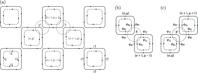
Figure 1: (a) The $\mathbb{Z}^{\ }_{2}$ network model. The solid and dashed lines represent the links for up and down spin electrons, respectively. The electrons are unitarily scattered at the nodes $\mathsf{S}$ and $\mathsf{S}^{\prime}$. The choice for the scattering basis at the nodes $\mathsf{S}$ and $\mathsf{S}^{\prime}$ is shown in (b) and (c), respectively.

The $\mathbb{Z}^{\ }_{2}$ network model is defined as follows. First, one draws a set of corner sharing square plaquettes on the two-dimensional Cartesian plane. Each edge of a plaquette is assigned two opposite directed links. This is the network. There are two types $\mathsf{S}$ and $\mathsf{S}^{\prime}$ of shared corners, which we shall call the nodes of the network. Second, we assign to each directed link an amplitude $\psi$, i.e., a complex number $\psi\in\mathbb{C}$. Any amplitude $\psi$ is either an incoming or outgoing plane wave that undergoes a unitary scattering process at a node. We also assign a $4\times 4$ unitary matrix $S$ to each node of the network. The set of all directed links obeying the condition that they are either the incoming or outgoing plane waves of the set of all nodal unitary scattering matrices defines a solution to the $\mathbb{Z}^{\ }_{2}$ network model.

To construct an explicit representation of the $\mathbb{Z}^{\ }_{2}$ network model, the center of each plaquette is assigned the coordinate $(x,y)$ with $x$ and $y$ taking integer values, as is done in figure 1. We then label the 8 directed links $\psi^{\ }_{n\sigma}(x,y)$ of any given plaquette by the coordinate $(x,y)$ of the plaquette, the side $n=1,2,3,4$ of the plaquette with the convention shown in figure 1, and the spin index $\sigma=\uparrow$ or $\sigma=\downarrow$ if the link is directed counterclockwise or clockwise, respectively, relative to the center of the plaquette. The $4\times 4$ unitary $S$-matrix is then given by

$$\left(\begin{array}[]{c}\psi^{\ }_{2\uparrow}(x,y)\\ \psi^{\ }_{3\downarrow}(x,y)\\ \psi^{\ }_{4\uparrow}(x+1,y-1)\\ \psi^{\ }_{1\downarrow}(x+1,y-1)\\ \end{array}\right)=:S\left(\begin{array}[]{c}\psi^{\ }_{3\uparrow}(x,y)\\ \psi^{\ }_{2\downarrow}(x,y)\\ \psi^{\ }_{1\uparrow}(x+1,y-1)\\ \psi^{\ }_{4\downarrow}(x+1,y-1)\\ \end{array}\right)$$ (1)

at any node of type $\mathsf{S}$ or as

$$\left(\begin{array}[]{c}\psi^{\ }_{3\uparrow}(x+1,y+1)\\ \psi^{\ }_{4\downarrow}(x+1,y+1)\\ \psi^{\ }_{1\uparrow}(x,y)\\ \psi^{\ }_{2\downarrow}(x,y)\\ \end{array}\right)=:S^{\prime}\left(\begin{array}[]{c}\psi^{\ }_{4\uparrow}(x+1,y+1)\\ \psi^{\ }_{3\downarrow}(x+1,y+1)\\ \psi^{\ }_{2\uparrow}(x,y)\\ \psi^{\ }_{1\downarrow}(x,y)\\ \end{array}\right)$$ (2)

at any node of type $\mathsf{S}^{\prime}$, with

$$S=U(x,y)S_{0}V(x,y),\qquad S^{\prime}=U^{\prime}(x,y)S_{0}V^{\prime}(x,y).$$ (3)

Here, the $4\times 4$ unitary matrix

$$S_{0}:=\left(\begin{array}[]{cc}rs^{\ }_{0}&tQ\\ -tQ^{{\dagger}}&rs^{\ }_{0}\end{array}\right)$$ (4)

is presented with the help of the unit $2\times 2$ matrix $s^{\ }_{0}$ and of the $2\times 2$ matrix

$$Q:=s^{\ }_{1}\sin\theta+s^{\ }_{3}\cos\theta=\left(\begin{array}[]{cc}\cos\theta&\sin\theta\\ \sin\theta&-\cos\theta\end{array}\right),$$ (5)

($s^{\ }_{1}$, $s^{\ }_{2}$, and $s^{\ }_{3}$ are the $2\times 2$ Pauli matrices) that are both acting on the spin indices $\sigma=\uparrow,\downarrow$, together with the real-valued parameters

$$r:=\tanh X,\qquad t:=\frac{1}{\cosh X},$$ (6)

with

$$\left\{(X,\theta)\,|\,0\leq X\leq\infty,\quad 0\leq\theta\leq\pi/2\right\}\!.$$ (7)

For later use, we shall also introduce the real-valued parameter $\beta\in[0,\pi]$ through

$$r=\cos\beta,\qquad t=\sin\beta.$$ (8)

The parameter $\theta$ controls the probability of spin-flip scattering, $\sin^{2}\theta$. The unitary matrices $U,V,U^{\prime},V^{\prime}$ are defined as

$$U(x,y)=\mathrm{diag}(\rme^{\rmi\chi^{\ }_{2}(x,y)},\rme^{\rmi\chi^{\ }_{3}(x,y)},\rme^{\rmi\chi^{\ }_{4}(x+1,y-1)},\rme^{\rmi\chi^{\ }_{1}(x+1,y-1)}),$$ (9a)

$$V(x,y)=\mathrm{diag}(\rme^{\rmi\chi^{\ }_{3}(x,y)},\rme^{\rmi\chi^{\ }_{2}(x,y)},\rme^{\rmi\chi^{\ }_{1}(x+1,y-1)},\rme^{\rmi\chi^{\ }_{4}(x+1,y-1)}),$$ (9b)

$$U^{\prime}(x,y)=\mathrm{diag}(\rme^{\rmi\chi^{\ }_{3}(x+1,y+1)},\rme^{\rmi\chi^{\ }_{4}(x+1,y+1)},\rme^{\rmi\chi^{\ }_{1}(x,y)},\rme^{\rmi\chi^{\ }_{2}(x,y)}),$$ (9c)

$$V^{\prime}(x,y)=\mathrm{diag}(\rme^{\rmi\chi^{\ }_{4}(x+1,y+1)},\rme^{\rmi\chi^{\ }_{3}(x+1,y+1)},\rme^{\rmi\chi^{\ }_{2}(x,y)},\rme^{\rmi\chi^{\ }_{1}(x,y)}),$$ (9d)

where $2\chi^{\ }_{n}(x,y)$ equals a (random) phase that wave functions acquire when propagating along the edge $n$ of the plaquette centered at $(x,y)$.

The $\mathbb{Z}^{\ }_{2}$ network model is uniquely defined from the scattering matrices $S$ and $S^{\prime}$. By construction, the $S$-matrix is time-reversal symmetric, i.e.,

$$\left(\begin{array}[]{cc}\mathrm{i}s^{\ }_{2}&0\\ 0&\mathrm{i}s^{\ }_{2}\end{array}\right)S^{*}\left(\begin{array}[]{cc}-\mathrm{i}s^{\ }_{2}&0\\ 0&-\mathrm{i}s^{\ }_{2}\end{array}\right)=S^{{\dagger}},$$ (9j)

and a similar relation holds for $S^{\prime}$.

In [19], we obtained the phase diagram of the $\mathbb{Z}^{\ }_{2}$ network model shown schematically in figure 2(a). Thereto, $(X,\theta)$ are spatially uniform deterministic parameters that can be changed continuously. On the other hand, the phases $\chi^{\ }_{n}$ of all link plane waves in the $\mathbb{Z}^{\ }_{2}$ network model are taken to be independently and uniformly distributed random variables over the range $[0,2\pi)$. The line $\theta=0$ is special in that the $\mathbb{Z}^{\ }_{2}$ network model reduces to two decoupled Chalker-Coddington network models [19]. Along the line $\theta=0$, the point

$$X^{\ }_{\mathrm{CC}}=\ln(1+\sqrt{2})\Longleftrightarrow\beta=\frac{\pi}{4}$$ (9k)

realizes a quantum critical point that separates two insulating phases differing by one gapless edge state or, equivalently, by one unit in the Hall conductivity, per spin. Alternatively, $\theta$ can also be chosen to be randomly and independently distributed at each node with the probability $\sin(2\theta)$ over the range $(0,\pi/2)$. This leaves $X$ as the sole deterministic parameter that controls the phase diagram as shown in figure 2(b). When performing numerically a scaling analysis with the size of the $\mathbb{Z}^{\ }_{2}$ network model, one must account for the deviations away from one-parameter scaling induced by irrelevant operators. The $\mathbb{Z}^{\ }_{2}$ network model with a randomly distributed $\theta$ minimizes such finite-size effects (see [19]).

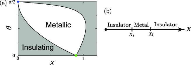
Figure 2: (a) Schematic phase diagram from the analysis of the $\mathbb{Z}^{\ }_{2}$ network model with the constant $X$ and $\theta$. The metallic phase is surrounded by the two insulating phases with the critical points $X_{s}$ and $X_{l}(>X_{s}))$ for $0<\theta<\pi/2$. The fixed point denoted by a filled (green) square along the boundary $\theta=0$ is the unstable quantum critical point located at $X^{\ }_{\mathrm{CC}}=\ln(1+\sqrt{2})$ separating two insulating phases in the Chalker-Coddington model. The fixed point denoted by the filled (blue) rhombus at the upper left corner is the unstable metallic phase. The shape of the metallic phase is controlled by the symmetry crossover between the unitary and symplectic symmetry classes. (b) The phase diagram for $\mathbb{Z}^{\ }_{2}$ network model with randomly distributed $\theta$ over the range $(0,\pi/2)$.

3 Two-dimensional Dirac Hamiltonian from the $\mathbb{Z}^{\ }_{2}$ network model

The Chalker-Coddington model is related to the two-dimensional Dirac Hamiltonian as was shown by Ho and Chalker in [32]. We are going to establish the counterpart of this connection for the $\mathbb{Z}^{\ }_{2}$ network model. A unitary matrix is the exponential of a Hermitian matrix. Hence, our strategy to construct a Hamiltonian from the $\mathbb{Z}^{\ }_{2}$ network model is going to be to view the unitary scattering matrix of the $\mathbb{Z}^{\ }_{2}$ network model as a unitary time evolution whose infinitesimal generator is the seeked Hamiltonian. To this end, we proceed in two steps in order to present the $\mathbb{Z}^{\ }_{2}$ network model into a form in which it is readily interpreted as a unitary time evolution. First, we change the choice of the basis for the scattering states and select the proper unit of time. We then perform a continuum approximation, by which the $\mathbb{Z}^{\ }_{2}$ network model is linearized, so to say. This will yield an irreducible 4-dimensional representation of the Dirac Hamiltonian in $(2+1)$-dimensional space and time, a signature of the fermion doubling when deriving a continuum Dirac Hamiltonian from a time-reversal symmetric and local two-dimensional lattice model.

3.1 Change of the basis for the scattering states and one-step time evolution

Our goal is to reformulate the $\mathbb{Z}^{\ }_{2}$ network model defined in Sec. 2 in such a way that the scattering matrix maps incoming states into outgoing states sharing the same internal and space labels but a different “time” label. This involves a change of basis for the scattering states and an “enlargement” of the Hilbert space spanned by the scattering states. The parameter $\theta$ is assumed to be spatially uniform. We choose the plaquette $(x,y)$ of the network.

At node $\mathsf{S}$ of the plaquette $(x,y)$, we make the basis transformation and write the $S$-matrix (1) in the form

$$\left(\begin{array}[]{c}\psi^{\ }_{1\downarrow}\\ \psi^{\ }_{3\downarrow}\\ \psi^{\ }_{2\uparrow}\\ \psi^{\ }_{4\uparrow}\\ \end{array}\right)=:\mathcal{M}^{\ }_{\mathsf{S}}\left(\begin{array}[]{c}\psi^{\ }_{1\uparrow}\\ \psi^{\ }_{3\uparrow}\\ \psi^{\ }_{2\downarrow}\\ \psi^{\ }_{4\downarrow}\\ \end{array}\right),\qquad\mathcal{M}^{\ }_{\mathsf{S}}=\mathcal{U}\,\mathcal{N}^{\ }_{\mathsf{S}}\,\mathcal{U},$$ (9l)

where we have defined

$$\mathcal{N}^{\ }_{\mathsf{S}}=\left(\begin{array}[]{cccc}0&-t\,t^{x}_{-}t^{y}_{+}\sin\theta&t\,t^{x}_{-}t^{y}_{+}\cos\theta&r\\ \!\!t\,t^{x}_{+}t^{y}_{-}\sin\theta&0&r&-t\,t^{x}_{+}t^{y}_{-}\cos\theta\!\!\\ t\,t^{x}_{+}t^{y}_{-}\cos\theta&r&0&t\,t^{x}_{+}t^{y}_{-}\sin\theta\\ r&-t\,t^{x}_{-}t^{y}_{+}\cos\theta&-t\,t^{x}_{-}t^{y}_{+}\sin\theta&0\end{array}\right)$$ (9m)

and

$$\mathcal{U}(x,y)=\mathrm{diag}(\rme^{\rmi\chi^{\ }_{1}(x,y)},\rme^{\rmi\chi^{\ }_{3}(x,y)},\rme^{\rmi\chi^{\ }_{2}(x,y)},\rme^{\rmi\chi^{\ }_{4}(x,y)}).$$ (9n)

Here given $n=1,2,3,4$ and $\sigma=\uparrow,\downarrow$, we have introduced the shift operators acting on $\psi^{\ }_{n\sigma}(x,y)$,

$$t^{x}_{\pm}\psi^{\ }_{n\sigma}(x,y):=\psi^{\ }_{n\sigma}(x\pm 1,y),\qquad t^{y}_{\pm}\psi^{\ }_{n\sigma}(x,y):=\psi^{\ }_{n}(x,y\pm 1),$$ (9o)

and similarly on the phases $\chi^{\ }_{n}(x,y)\in[0,2\pi)$. We note that the scattering matrix $\mathcal{N}_{\mathsf{S}}$ is multiplied by the unitary matrix $\mathcal{U}$ from the left and the right in (9l), because the Kramers’ doublet acquires exactly the same phase $\chi_{n}$ when traversing on the edge $n$ of the plaquette $(x,y)$ before and after experiencing the scattering $\mathcal{N}_{\mathsf{S}}$ at the node $\mathsf{S}$.

At node $\mathsf{S}^{\prime}$ of the plaquette $(x,y)$, we make the basis transformation and rewrite the scattering matrix $S^{\prime}$ (2) into the form

$$\left(\begin{array}[]{c}\psi^{\ }_{1\uparrow}\\ \psi^{\ }_{3\uparrow}\\ \psi^{\ }_{2\downarrow}\\ \psi^{\ }_{4\downarrow}\\ \end{array}\right)=:\mathcal{M}^{\ }_{\mathsf{S}^{\prime}}\left(\begin{array}[]{c}\psi^{\ }_{1\downarrow}\\ \psi^{\ }_{3\downarrow}\\ \psi^{\ }_{2\uparrow}\\ \psi^{\ }_{4\uparrow}\\ \end{array}\right),\qquad\mathcal{M}^{\ }_{\mathsf{S}^{\prime}}=\mathcal{U}\,\mathcal{N}^{\ }_{\mathsf{S}^{\prime}}\,\mathcal{U},$$ (9p)

where we have defined

$$\mathcal{N}^{\ }_{\mathsf{S}^{\prime}}=\!\left(\begin{array}[]{cccc}0&-t\,t^{x}_{+}t^{y}_{+}\sin\theta&r&-t\,t^{x}_{+}t^{y}_{+}\cos\theta\!\\ t\,t^{x}_{-}t^{y}_{-}\sin\theta&0&t\,t^{x}_{-}t^{y}_{-}\cos\theta&r\\ r&t\,t^{x}_{+}t^{y}_{+}\cos\theta&0&-t\,t^{x}_{+}t^{y}_{+}\sin\theta\\ \!\!\!-t\,t^{x}_{-}t^{y}_{-}\cos\theta&r&t\,t^{x}_{-}t^{y}_{-}\sin\theta&0\end{array}\right).$$ (9q)

As it should be

$$\mathcal{M}^{{\dagger}}_{\mathsf{S}}\mathcal{M}^{\ }_{\mathsf{S}}=\mathcal{M}^{{\dagger}}_{\mathsf{S}^{\prime}}\mathcal{M}^{\ }_{\mathsf{S}^{\prime}}=1.$$ (9r)

Next, we introduce the discrete time variable $l\in\mathbb{Z}$ as follows. We define the elementary discrete unitary time evolution to be

$$\left(\begin{array}[]{c}\psi^{\ }_{+\downarrow}\\ \psi^{\ }_{-\uparrow}\\ \psi^{\ }_{+\uparrow}\\ \psi^{\ }_{-\downarrow}\end{array}\right)^{\ }_{l+1}:=\left(\begin{array}[]{cc}0&\mathcal{M}^{\ }_{\mathsf{S}}\\ \mathcal{M}^{\ }_{\mathsf{S}^{\prime}}&0\end{array}\right)\left(\begin{array}[]{c}\psi^{\ }_{+\downarrow}\\ \psi^{\ }_{-\uparrow}\\ \psi^{\ }_{+\uparrow}\\ \psi^{\ }_{-\downarrow}\end{array}\right)^{\ }_{l}.$$ (9ac)

Here, to treat on equal footing the nodes of type $\mathsf{S}$ and $\mathsf{S}^{\prime}$, we have enlarged the scattering basis with the introduction of the doublets

$$\psi^{\ }_{+} := \left(\begin{array}[]{c}\psi^{\ }_{1}\\ \psi^{\ }_{3}\end{array}\right),\qquad\psi^{\ }_{-}:=\left(\begin{array}[]{c}\psi^{\ }_{2}\\ \psi^{\ }_{4}\end{array}\right).$$ (9ah)

Due to the off-diagonal block structure in the elementary time evolution, it is more convenient to consider the “one-step” time evolution operator defined by

$$\left(\begin{array}[]{c}\psi^{\ }_{+\downarrow}\\ \psi^{\ }_{-\uparrow}\\ \psi^{\ }_{+\uparrow}\\ \psi^{\ }_{-\downarrow}\end{array}\right)^{\ }_{l+2} = \left(\begin{array}[]{cc}\mathcal{M}^{\ }_{\mathsf{S}}\mathcal{M}^{\ }_{\mathsf{S}^{\prime}}&0\\ 0&\mathcal{M}^{\ }_{\mathsf{S}^{\prime}}\mathcal{M}^{\ }_{\mathsf{S}}\end{array}\right)\left(\begin{array}[]{c}\psi^{\ }_{+\downarrow}\\ \psi^{\ }_{-\uparrow}\\ \psi^{\ }_{+\uparrow}\\ \psi^{\ }_{-\downarrow}\end{array}\right)^{\ }_{l}$$ (9as)

$$\equiv \left(\begin{array}[]{cc}\mathcal{M}^{\ }_{\mathsf{S}\mathsf{S}^{\prime}}&0\\ 0&\mathcal{M}^{\ }_{\mathsf{S}^{\prime}\mathsf{S}}\end{array}\right)\left(\begin{array}[]{c}\psi^{\ }_{+\downarrow}\\ \psi^{\ }_{-\uparrow}\\ \psi^{\ }_{+\uparrow}\\ \psi^{\ }_{-\downarrow}\end{array}\right)^{\ }_{l}.$$ (9az)

The two Hamiltonians generating this unitary time evolution are then

$$\mathcal{H}^{\ }_{\mathsf{S}\mathsf{S}^{\prime}}:=+\mathrm{i}\ln\mathcal{M}^{\ }_{\mathsf{S}\mathsf{S}^{\prime}},\qquad\mathcal{H}^{\ }_{\mathsf{S}^{\prime}\mathsf{S}}:=+\mathrm{i}\ln\mathcal{M}^{\ }_{\mathsf{S}^{\prime}\mathsf{S}}.$$ (9ba)

Evidently, the additivity of the logarithm of a product implies that

$$\mathcal{H}^{\ }_{\mathsf{S}\mathsf{S}^{\prime}}=\mathcal{H}^{\ }_{\mathsf{S}^{\prime}\mathsf{S}}.$$ (9bb)

From now on, we will consider $\mathcal{H}^{\ }_{\mathsf{S}\mathsf{S}^{\prime}}$ exclusively since $\mathcal{M}^{\ }_{\mathsf{S}^{\prime}\mathsf{S}}=\exp(\mathrm{i}\mathcal{H}^{\ }_{\mathsf{S}^{\prime}\mathsf{S}})$ merely duplicates the information contains in $\mathcal{M}^{\ }_{\mathsf{S}\mathsf{S}^{\prime}}=\exp(\mathrm{i}\mathcal{H}^{\ }_{\mathsf{S}\mathsf{S}^{\prime}})$.

3.2 Dirac Hamiltonian close to $\theta=0$

In this section, we are going to extract from the unitary time-evolution (9az)–(9bb) of the $\mathbb{Z}^{\ }_{2}$ network model a $4\times 4$ continuum Dirac Hamiltonian in the close vicinity of the quantum critical point

$$(\theta,\beta)^{\ }_{\mathrm{CC}}:=(0,\pi/4).$$ (9bc)

To this end and following [32], it is convenient to measure the link phases $\chi^{\ }_{n}$ ($n=1,2,3,4$) relative to their values when they carry a flux of $\pi$ per plaquette. Hence, we redefine

$$\chi^{\ }_{4}\to\chi^{\ }_{4}+\frac{\pi}{2}$$ (9bd)

on all plaquettes.

Our strategy consists in performing an expansion of

$$\mathcal{H}^{\ }_{\mathsf{S}\mathsf{S}^{\prime}}=+\mathrm{i}\ln\mathcal{M}^{\ }_{\mathsf{S}\mathsf{S}^{\prime}}=+\mathrm{i}\left(\ln\mathcal{M}^{\ }_{\mathsf{S}}+\ln\mathcal{M}^{\ }_{\mathsf{S}}\right)=+\mathrm{i}\ln\mathcal{M}^{\ }_{\mathsf{S}^{\prime}\mathsf{S}}=\mathcal{H}^{\ }_{\mathsf{S}^{\prime}\mathsf{S}}$$ (9be)

defined in (9ba) to leading order in powers of

$$\theta,\quad\frac{m}{2}\equiv\beta-\frac{\pi}{4},\quad\partial_{x,y}\equiv\ln t^{x,y}_{+},\quad\chi^{\ }_{n}$$ (9bf)

with $n=1,2,3,4$ where $\partial_{x,y}$ is the generator of infinitesimal translation on the network (the two-dimensional momentum operator).

When $\theta=0$, the unitary time-evolution operator at the plaquette $(x,y)$ is given by

$$\left(\begin{array}[]{c}\psi^{\ }_{+\downarrow}\\ \psi^{\ }_{-\uparrow}\\ \end{array}\right)^{\ }_{l+2}=\mathcal{M}^{(0)}_{\mathsf{S}\mathsf{S}^{\prime}}\left(\begin{array}[]{c}\psi^{\ }_{+\downarrow}\\ \psi^{\ }_{-\uparrow}\\ \end{array}\right)^{\ }_{l},$$ (9bk)

$$\mathcal{M}^{(0)}_{\mathsf{S}\mathsf{S}^{\prime}}=\left(\begin{array}[]{cc}A^{(0)}D^{(0)}&0\\ 0&B^{(0)}C^{(0)}\end{array}\right),$$ (9bn)

whereby

$$\mathcal{M}^{(0)}_{\mathsf{S}\mathsf{S}^{\prime}}=\mathcal{M}^{(0)}_{\mathsf{S}}\mathcal{M}^{(0)}_{\mathsf{S}^{\prime}},$$ (9bo)

$$\mathcal{M}^{(0)}_{\mathsf{S}}=\left(\begin{array}[]{cc}0&A^{(0)}\\ B^{(0)}&0\end{array}\right),\qquad\mathcal{M}^{(0)}_{\mathsf{S}^{\prime}}=\left(\begin{array}[]{cc}0&C^{(0)}\\ D^{(0)}&0\end{array}\right),$$ (9bt)

with the $2\times 2$ operator-valued matrices

$$A^{(0)} := \left(\begin{array}[]{cc}\!\rme^{\rmi\chi^{\ }_{1}}t^{x}_{-}t^{y}_{+}\rme^{\rmi\chi^{\ }_{2}}\sin\beta&\rmi\rme^{\rmi(\chi^{\ }_{1}+\chi^{\ }_{4})}\cos\beta\\ \rme^{\rmi(\chi^{\ }_{3}+\chi^{\ }_{2})}\cos\beta&-\rmi\rme^{\rmi\chi^{\ }_{3}}t^{x}_{+}t^{y}_{-}\rme^{\rmi\chi^{\ }_{4}}\sin\beta\!\end{array}\right),$$ (9bw)

$$B^{(0)} := \left(\begin{array}[]{cc}\rme^{\rmi\chi^{\ }_{2}}t^{x}_{+}t^{y}_{-}\rme^{\rmi\chi^{\ }_{1}}\sin\beta&\rme^{\rmi(\chi^{\ }_{2}+\chi^{\ }_{3})}\cos\beta\\ \rmi\rme^{\rmi(\chi^{\ }_{4}+\chi^{\ }_{1})}\cos\beta&-\rmi\rme^{\rmi\chi^{\ }_{4}}t^{x}_{-}t^{y}_{+}\rme^{\rmi\chi^{\ }_{3}}\sin\beta\end{array}\right),$$ (9bz)

$$C^{(0)} := \left(\begin{array}[]{cccc}\rme^{\mathrm{i}(\chi^{\ }_{1}+\chi^{\ }_{2})}\cos\beta&-\rmi\rme^{\mathrm{i}\chi^{\ }_{1}}t^{x}_{+}t^{y}_{+}\rme^{\mathrm{i}\chi^{\ }_{4}}\sin\beta\\ \!\rme^{\mathrm{i}\chi^{\ }_{3}}t^{x}_{-}t^{y}_{-}\rme^{\mathrm{i}\chi^{\ }_{2}}\sin\beta&\rmi\rme^{\mathrm{i}(\chi^{\ }_{3}+\chi^{\ }_{4})}\cos\beta\\ \end{array}\right),$$ (9cc)

$$D^{(0)} := \left(\begin{array}[]{cc}\rme^{\rmi(\chi^{\ }_{2}+\chi^{\ }_{1})}\cos\beta&\rme^{\rmi\chi^{\ }_{2}}t^{x}_{+}t^{y}_{+}\rme^{\rmi\chi^{\ }_{3}}\sin\beta\!\\ \!-\rmi\rme^{\rmi\chi^{\ }_{4}}t^{x}_{-}t^{y}_{-}\rme^{\rmi\chi^{\ }_{1}}\sin\beta&\rmi\rme^{\rmi(\chi^{\ }_{4}+\chi^{\ }_{3})}\cos\beta\end{array}\right).$$ (9cf)

Observe that in the limit $\theta=0$, the $\mathbb{Z}^{\ }_{2}$ network model reduces to two decoupled U(1) network models where each time evolution is essentially the same as the one for the U(1) network model derived in [32].

In the vicinity of the Chalker-Coddington quantum critical point (9bc), we find the $4\times 4$ block diagonal Hamiltonian

$$\mathcal{H}^{(0)}_{\mathsf{S}\mathsf{S}^{\prime}}=\left(\begin{array}[]{cc}D^{\ }_{+}&0\\ 0&D^{\ }_{-}\\ \end{array}\right)$$ (9ci)

where the $2\times 2$ block are expressed in terms of linear combinations of the $2\times 2$ unit matrix $\sigma^{\ }_{0}$ and of the Pauli matrices $\sigma^{\ }_{x}$, $\sigma^{\ }_{y}$, and $\sigma^{\ }_{z}$ according to

$$D^{\ }_{+}=\sigma^{\ }_{z}\left(-\rmi\partial^{\ }_{x}+A^{\ }_{x}\right)-\sigma^{\ }_{x}\left(-\rmi\partial^{\ }_{y}+A^{\ }_{y}\right)-\sigma^{\ }_{y}m+\sigma^{\ }_{0}A^{\ }_{0},$$ (9cj)

and

$$D^{\ }_{-}=-\sigma^{\ }_{y}\left(-\rmi\partial^{\ }_{x}-A^{\ }_{x}\right)+\sigma^{\ }_{z}\left(-\rmi\partial^{\ }_{y}-A^{\ }_{y}\right)+\sigma^{\ }_{x}m+\sigma^{\ }_{0}A^{\ }_{0}.$$ (9ck)

Thus, each $2\times 2$ block Hamiltonian is of the Dirac form whereby the linear combinations

$$A^{\ }_{0}:=-(\chi^{\ }_{1}+\chi^{\ }_{2}+\chi^{\ }_{3}+\chi^{\ }_{4}),\qquad(A^{\ }_{x},A^{\ }_{y}):=(-\chi^{\ }_{1}+\chi^{\ }_{3},\chi^{\ }_{2}-\chi^{\ }_{4}),$$ (9cl)

enter as a scalar gauge potential and a vector gauge potential would do, respectively.

Any deviation of $\theta$ from $\theta=0$ lifts the reducibility of (9ci). To leading order in $\theta$ and close to the Chalker-Coddington quantum critical point (9bc),

$$\mathcal{M}^{\ }_{\mathsf{S}\mathsf{S}^{\prime}} = \left(\mathcal{M}^{(0)}_{\mathsf{S}}+\theta\mathcal{M}^{(1)}_{\mathsf{S}}+\cdots\right)\left(\mathcal{M}^{(0)}_{\mathsf{S}^{\prime}}+\theta\mathcal{M}^{(1)}_{\mathsf{S}^{\prime}}+\cdots\right)$$ (9cm)

$$= \mathcal{M}^{(0)}_{\mathsf{S}\mathsf{S}^{\prime}}+\theta\left(\mathcal{M}^{(1)}_{\mathsf{S}}\mathcal{M}^{(0)}_{\mathsf{S}^{\prime}}+\mathcal{M}^{(0)}_{\mathsf{S}}\mathcal{M}^{(1)}_{\mathsf{S}^{\prime}}\right)+\cdots$$

with

$$\mathcal{M}^{(1)}_{\mathsf{S}}=\left(\begin{array}[]{cccc}A^{(1)}&0\\ 0&B^{(1)}\end{array}\right)\!,\qquad A^{(1)}=\frac{1}{\sqrt{2}}\left(\begin{array}[]{cccc}0&-1\\ 1&0\end{array}\right)\!,\qquad B^{(1)}=\frac{1}{\sqrt{2}}\left(\begin{array}[]{cccc}0&\rmi\\ -\rmi&0\end{array}\right)\!,$$ (9ct)

$$\mathcal{M}^{(1)}_{\mathsf{S}^{\prime}}=\left(\begin{array}[]{cccc}C^{(1)}&0\\ 0&D^{(1)}\end{array}\right)\!,\qquad C^{(1)}=\frac{1}{\sqrt{2}}\left(\begin{array}[]{cccc}0&-1\\ 1&0\end{array}\right)\!,\qquad D^{(1)}=\frac{1}{\sqrt{2}}\left(\begin{array}[]{cccc}0&-\rmi\\ \rmi&0\end{array}\right)\!,$$ (9da)

where we have set $m=\chi^{\ }_{n}=0$ and $t^{x,y}_{\pm}=1$. We obtain

$$\mathcal{H}^{\ }_{\mathsf{S}\mathsf{S}^{\prime}}=\left(\begin{array}[]{cc}D^{\ }_{+}&D^{\ }_{\theta}\\ D^{{\dagger}}_{\theta}&D^{\ }_{-}\end{array}\right),\qquad D^{\ }_{\theta}:=\theta\left(\begin{array}[]{cc}-\rmi&1\\ \rmi&1\end{array}\right)$$ (9df)

to this order.

Next, we perform a sequence of unitary transformation generated by

$$U=\left(\begin{array}[]{cc}\rme^{\rmi\pi\sigma^{\ }_{y}/4}&0\\ 0&\rme^{\rmi\pi\sigma^{\ }_{z}/4}\\ \end{array}\right)\left(\begin{array}[]{cc}\rme^{-\rmi\pi\sigma^{\ }_{x}/4}&0\\ 0&\rme^{-\rmi\pi\sigma^{\ }_{x}/4}\\ \end{array}\right)\left(\begin{array}[]{cc}\rme^{-\rmi\pi/8}&0\\ 0&\rme^{\rmi\pi/8}\\ \end{array}\right),$$ (9dg)

yielding

$$\mathcal{H}:=U^{\dagger}\mathcal{H}^{\ }_{\mathsf{S}\mathsf{S}^{\prime}}U=\left(\begin{array}[]{cc}\mathcal{H}^{\ }_{+}&\alpha\sigma^{\ }_{0}\\ \alpha\sigma^{\ }_{0}&\mathcal{H}^{\ }_{-}\\ \end{array}\right)$$ (9dh)

with $\alpha=\sqrt{2}\theta$ and

$$\mathcal{H}^{\ }_{\pm}=\sigma^{\ }_{x}\left(-\rmi\partial^{\ }_{x}\pm A^{\ }_{x}\right)+\sigma^{\ }_{y}\left(-\rmi\partial^{\ }_{y}\pm A^{\ }_{y}\right)\pm\sigma^{\ }_{z}m+\sigma^{\ }_{0}A^{\ }_{0}.$$ (9di)

The $2\times 2$ matrices $\mathcal{H}^{\ }_{+}$ and $\mathcal{H}^{\ }_{-}$ describe a Dirac fermion with mass $\pm m$ in the presence of random vector potential $\pm(A^{\ }_{x},A^{\ }_{y})$ and random scalar potential $A^{\ }_{0}$, each of which is an effective Hamiltonian for the plateau transition of integer quantum Hall effect [32, 33]. The $\mathcal{H}^{\ }_{\pm}$ sectors are coupled by the matrix element $\alpha\sigma^{\ }_{0}$.

The $4\times 4$ continuum Dirac Hamiltonian $\mathcal{H}$ can be written in the form

$$\mathcal{H}= (-\rmi\partial^{\ }_{x}\sigma^{\ }_{x}-\rmi\partial^{\ }_{y}\sigma^{\ }_{y})\otimes\tau^{\ }_{0}+(A^{\ }_{x}\sigma^{\ }_{x}+A^{\ }_{y}\sigma^{\ }_{y}+m\sigma^{\ }_{z})\otimes\tau^{\ }_{z}$$ (9dj)

$$+A^{\ }_{0}\sigma^{\ }_{0}\otimes\tau^{\ }_{0}+\alpha\,\sigma^{\ }_{0}\otimes\tau^{\ }_{x},$$

where $\tau^{\ }_{0}$ is a unit $2\times 2$ matrix and $\tau^{\ }_{x}$, $\tau^{\ }_{y}$, and $\tau^{\ }_{z}$ are three Pauli matrices. The Hamiltonian (9dj) is invariant for each realization of disorder under the operation

$$T\,\mathcal{H}^{*}\,T^{-1}=\mathcal{H},\qquad T:=\rmi\sigma^{\ }_{y}\otimes\tau^{\ }_{x},$$ (9dk)

that implements time-reversal for a spin-1/2 particle.

The Dirac Hamiltonian (9dj) is the main result of this subsection. It is an effective model for the Anderson localization of quantum spin Hall systems, which belongs to the symplectic class in view of the symmetry property (9dk). The Anderson transition in the Dirac Hamiltonian (9dj) should possess the same universal critical properties as those found in our numerical simulations of the $\mathbb{Z}^{\ }_{2}$ network model. In the presence of the “Rashba” coupling $\alpha$, there should appear a metallic phase near $m=0$ which is surrounded by two insulating phases. In the limit $\alpha\to 0$, the metallic phase should shrink into a critical point of the integer quantum Hall plateau transition.

The $4\times 4$ continuum Dirac Hamiltonian $\mathcal{H}$ should be contrasted with a $2\times 2$ Hamiltonian of a Dirac particle in random scalar potential,

$$\mathcal{H}^{\ }_{2}=-\rmi\partial^{\ }_{x}\sigma^{\ }_{x}-\rmi\partial^{\ }_{y}\sigma^{\ }_{y}+V(x,y)\sigma^{\ }_{0},$$ (9dl)

which has the minimal dimensionality of the Clifford algebra in $(2+1)$-dimensional space time and is invariant under time-reversal operation, $\sigma^{\ }_{y}\mathcal{H}^{*}_{2}\sigma^{\ }_{y}=\mathcal{H}^{\ }_{2}$. The $2\times 2$ Dirac Hamiltonian (9dl) is an effective Hamiltonian for massless Dirac fermions on the surface of a three-dimensional $\mathbb{Z}^{\ }_{2}$ topological insulator. After averaging over the disorder potential $V$, the problem of Anderson localization of the surface Dirac fermions is reduced to a NLSM with a $\mathbb{Z}^{\ }_{2}$ topological term [25, 26]. Interestingly, this $\mathbb{Z}^{\ }_{2}$ topological term prevents the surface Dirac fermions from localizing [27, 28]. It is this absence of two-dimensional localization that defines a three-dimensional $\mathbb{Z}^{\ }_{2}$ topological insulator [29]. In contrast, the doubling of the size of the Hamiltonian (9dj) implies that the NLSM describing the Anderson localization in the $4\times 4$ Hamiltonian (9dh) does not come with a $\mathbb{Z}^{\ }_{2}$ topological term, because two $\mathbb{Z}^{\ }_{2}$ topological terms cancel each other. We can thus conclude that the critical properties of metal-insulator transitions in the $\mathbb{Z}^{\ }_{2}$ network model are the same as those in the standard symplectic class, in agreement with results of our numerical simulations of the $\mathbb{Z}^{\ }_{2}$ network model [19, 20].

Before closing this subsection, we briefly discuss the Dirac Hamiltonian (9dj) in the clean limit where $A^{\ }_{0}=A^{\ }_{x}=A^{\ }_{y}=0$. Since the system in the absence of disorder is translationally invariant, momentum is a good quantum number. We thus consider the Hamiltonian in momentum space

$$\mathcal{H}(\bi{k})=\left(\begin{array}[]{cc}k^{\ }_{x}\sigma^{\ }_{x}+k^{\ }_{y}\sigma^{\ }_{y}+m\sigma^{\ }_{z}&\alpha\sigma^{\ }_{0}\\ \alpha\sigma^{\ }_{0}&k^{\ }_{x}\sigma^{\ }_{x}+k^{\ }_{y}\sigma^{\ }_{y}-m\sigma^{\ }_{z}\end{array}\right),$$ (9dm)

where the wave number $\bi{k}=(k^{\ }_{x},k^{\ }_{y})$. When $\alpha=0$, the Hamiltonian (9dm) becomes a direct sum of $2\times 2$ Dirac Hamiltonian with mass of opposite signs. This is essentially the same low-energy Hamiltonian as the one appearing in the quantum spin Hall effect in HgTe/(Hg,Cd)Te quantum wells [6].

3.3 $\mathbb{Z}^{\ }_{2}$ topological number

We now discuss the topological property of the time-reversal invariant insulator which is obtained from the effective Hamiltonian (9dm) of the $\mathbb{Z}^{\ }_{2}$ network model in the absence of disorder. The topological attribute of the band insulator is intimately tied to the invariance

$$\hat{\Theta}^{-1}\mathcal{H}(-\bm{k})\hat{\Theta}=\mathcal{H}(\bm{k})$$ (9dn)

under the operation of time-reversal represented by

$$\hat{\Theta}:=(\rmi\sigma^{\ }_{y}\otimes\tau^{\ }_{x})\mathcal{K}=-\hat{\Theta}^{-1},$$ (9do)

where $\mathcal{K}$ implements complex conjugation. We are going to show that this topological attribute takes values in $\mathbb{Z}^{\ }_{2}$, i.e., the $\mathbb{Z}^{\ }_{2}$ index introduced by Kane and Mele [4].

We begin with general considerations on a translation-invariant single-particle fermionic Hamiltonian which has single-particle eigenstates labeled by the wave vector $\bm{k}$ taking values in a compact manifold. This compact manifold can be the first Brillouin zone with the topology of a torus if the Hamiltonian is defined on a lattice and periodic boundary conditions are imposed, or it can be the stereographic projection between the momentum plane $\mathbb{R}^{2}$ and the surface of a three-dimensional sphere if the Hamiltonian is defined in the continuum. We assume that (i) the antiunitary operation $\hat{\Theta}=-\hat{\Theta}^{-1}=-\Theta^{{\dagger}}$ that implements time-reversal leaves the Hamiltonian invariant, (ii) there exists a spectral gap at the Fermi energy, and (iii) there are two distinct occupied bands with the single-particle orthonormal eigenstates $|u^{\ }_{\hat{a}}(\bm{k})\rangle$ and energies $E^{\ }_{\hat{a}}(\bm{k})$ labeled by the index $\hat{a}=1,2$ below the Fermi energy. All three assumptions are met by the $4\times 4$ Dirac Hamiltonian (9dj), provided that the mass $m$ is nonvanishing.

Because of assumptions (i) and (ii) the $2\times 2$ unitary sewing matrix with the matrix elements $w_{\hat{a}\hat{b}}(\bi{k})$ defined by

$$w^{\ }_{\hat{a}\hat{b}}(\bm{k}):=\langle u^{\ }_{\hat{a}}(-\bm{k})|\bigg{(}\hat{\Theta}|u^{\ }_{\hat{b}}(\bm{k})\rangle\bigg{)}\equiv\left\langle u^{\ }_{\hat{a}}(-\bm{k})\left|\Theta u^{\ }_{\hat{b}}(\bm{k})\right.\right\rangle,\quad\hat{a},\hat{b}=1,2,$$ (9dp)

i.e., the overlaps between the occupied single-particle energy eigenstates with momentum $-\bm{k}$ and the time reversed images to the occupied single-particle energy eigenstates with momentum $\bm{k}$, plays an important role [17]. The matrix elements (9dp) obey

$$w^{\ }_{\hat{a}\hat{b}}(\bm{k}) \equiv\langle u^{\ }_{\hat{a}}(-\bm{k})|\bigg{(}\hat{\Theta}|u^{\ }_{\hat{b}}(\bm{k})\rangle\bigg{)}$$ (9dq)

$$=\langle u^{\ }_{\hat{b}}(\bm{k})|\bigg{(}\hat{\Theta}^{{\dagger}}|u^{\ }_{\hat{a}}(-\bm{k})\rangle\bigg{)}$$

$$=-\langle u^{\ }_{\hat{b}}(\bm{k})|\bigg{(}\hat{\Theta}|u^{\ }_{\hat{a}}(-\bm{k})\rangle\bigg{)}$$

$$\equiv-w^{\ }_{\hat{b}\hat{a}}(-\bm{k}),\qquad\qquad\qquad\qquad\hat{a},\hat{b}=1,2.$$

We used the fact that $\hat{\Theta}$ is antilinear to reach the second equality and that it is antiunitary with $\hat{\Theta}^{2}=-1$ to reach the third equality. Hence, the $2\times 2$ unitary sewing matrix $w(\bm{k})$ with the matrix elements (9dp) can be parametrized as

$$w(\bm{k})=\left(\begin{array}[]{cc}w^{\ }_{11}(\bm{k})&w^{\ }_{12}(\bm{k})\\ -w^{\ }_{12}(-\bm{k})&w^{\ }_{22}(\bm{k})\end{array}\right)=-w^{\mathrm{T}}(-\bm{k})$$ (9dr)

with the three complex-valued functions

$$w^{\ }_{11}(\bm{k})=-w^{\ }_{11}(-\bm{k}),\qquad w^{\ }_{22}(\bm{k})=-w^{\ }_{22}(-\bm{k}),\qquad w^{\ }_{12}(\bm{k}).$$ (9ds)

We observe that $w(\bi{k})$ reduces to

$$w(\bm{k})=e^{\rmi f(\bi{k})}\left(\begin{array}[]{cc}0&-1\\ +1&0\end{array}\right)$$ (9dt)

for some real-valued $f(\bm{k})$ at any time-reversal invariant wave vector $\bm{k}\sim-\bm{k}$ (time-reversal invariant wave vectors are half a reciprocal vector for a lattice model, and 0 or $\infty$ for a model in the continuum).

As we shall shortly see, the sewing matrix (9dp) imposes constraints on the U(2) Berry connection

$$\mathcal{A}^{\ }_{\hat{a}\hat{b}}(\bm{k}):=\left\langle u^{\ }_{\hat{a}}(\bm{k})\left|\mathrm{d}u^{\ }_{\hat{b}}(\bm{k})\right.\right\rangle\equiv\left\langle u^{\ }_{\hat{a}}(\bm{k})\left|\frac{\partial}{\partial k^{\ }_{\mu}}u^{\ }_{\hat{b}}(\bm{k})\right.\right\rangle\mathrm{d}k^{\ }_{\mu}\equiv A^{\mu}_{\hat{a}\hat{b}}(\bm{k})\mathrm{d}k^{\ }_{\mu},$$ (9du)

where the summation convention over the repeated index $\mu$ is understood (we do not make distinction between superscript and subscript). Here, at every point $\bm{k}$ in momentum space, we have introduced the U(2) antihermitian gauge field $A^{\ }_{\mu}(\bm{k})$ with the space index $\mu=1,2$ and the matrix elements

$$A^{\mu}_{\hat{a}\hat{b}}(\bm{k})=-\left(A^{\mu}_{\hat{b}\hat{a}}(\bm{k})\right)^{*}$$ (9dv)

labeled with the U(2) internal indices $\hat{a},\hat{b}=1,2$, by performing an infinitesimal parametric change in the Hamiltonian. We decompose the U(2) gauge field (9du) into the U(1) and the SU(2) contributions

$$A^{\ }_{\mu}(\bm{k})\equiv a^{0}_{\mu}(\bm{k})\frac{\rho^{\ }_{0}}{2\mathrm{i}}+\bm{a}^{\ }_{\mu}(\bm{k})\cdot\frac{\bm{\rho}}{2\mathrm{i}},$$ (9dw)

where $\rho^{\ }_{0}$ is a $2\times 2$ unit matrix and $\bm{\rho}$ is a 3 vector made of the Pauli matrices $\rho^{\ }_{x}$, $\rho^{\ }_{y}$, and $\rho^{\ }_{z}$. Accordingly,

$$\mathcal{A}^{\mathrm{U}(2)}(\bm{k}) = \mathcal{A}^{\mathrm{U}(1)}(\bm{k})+\mathcal{A}^{\mathrm{SU}(2)}(\bm{k}).$$ (9dx)

Combining the identity $\hat{\Theta}^{2}=-1$ with the (partial) resolution of the identity $\sum_{\hat{a}=1,2}|u^{\ }_{\hat{a}}(\bi{k})\rangle\langle u^{\ }_{\hat{a}}(\bi{k})|$ for the occupied energy eigenstates with momentum $\bi{k}$ yields

$$\sum_{\hat{a}=1,2}\hat{\Theta}|u^{\ }_{\hat{a}}(\bi{k})\rangle\langle u^{\ }_{\hat{a}}(\bi{k})|\hat{\Theta}=-1,$$ (9dy)

where the proper restriction to the occupied energy eigenstates is understood for the unit operator on the right-hand side. Using this identity, we deduce the gauge transformation

$$A^{\ }_{\mu}(-\bm{k}) =-\left(\left\langle u^{\ }_{\hat{a}}(-\bi{k})\left|\frac{\partial}{\partial k^{\ }_{\mu}}u^{\ }_{\hat{b}}(-\bi{k})\right.\right\rangle\right)^{\ }_{\hat{a},\hat{b}=1,2}$$ (9dz)

$$=-w(\bm{k})A^{*}_{\mu}(\bm{k})w^{{\dagger}}(\bm{k})-w(\bm{k})\partial^{\ }_{\mu}w^{{\dagger}}(\bm{k})$$

$$=+w(\bm{k})A^{\mathrm{T}}_{\mu}(\bm{k})w^{{\dagger}}(\bm{k})-w(\bm{k})\partial^{\ }_{\mu}w^{{\dagger}}(\bm{k})$$

that relates the U(2) connections at $\pm\bm{k}$. For the U(1) and SU(2) parts of the connection,

$$a^{0}_{\mu}(-\bm{k})=a^{0}_{\mu}(\bm{k})-2\partial^{\ }_{\mu}\zeta(\bm{k}),$$ (9ea)

$$\bm{a}^{\ }_{\mu}(-\bm{k})\cdot\bm{\rho}=\bm{a}^{\ }_{\mu}(\bm{k})\cdot\tilde{w}(\bm{k})\bm{\rho}^{\mathrm{T}}\tilde{w}^{{\dagger}}(\bm{k})-2\rmi\,\tilde{w}(\bm{k})\partial_{\mu}\tilde{w}^{{\dagger}}(\bm{k}),$$ (9eb)

where we have decomposed $w(k)$ into the U(1) ($\rme^{\mathrm{i}\zeta}$) and SU(2) ($\tilde{w}$) parts according to

$$w(\bm{k})=\rme^{\rmi\zeta(\bm{k})}\tilde{w}(\bm{k}),$$ (9ec)

(note that this decomposition has a global sign ambiguity, which, however, will not affect the following discussions).

Equipped with these gauge fields, we introduce the U(2) Wilson loop

$$W^{\ }_{\mathrm{U}(2)}[\mathcal{C}] :=\frac{1}{2}\mathrm{tr}\,\mathcal{P}\exp\left(\oint\limits_{\mathcal{C}}\mathcal{A}^{\mathrm{U}(2)}(\bm{k})\right)$$ (9ed)

$$=W^{\ }_{\mathrm{U}(1)}[\mathcal{C}]\times W^{\ }_{\mathrm{SU}(2)}[\mathcal{C}],$$

where the U(1) Wilson loop is given by

$$W^{\ }_{\mathrm{U}(1)}[\mathcal{C}]:=\exp\left(\oint\limits_{\mathcal{C}}\mathcal{A}^{\mathrm{U}(1)}(\bm{k})\right),$$ (9ee)

while the SU(2) Wilson loop is given by

$$W^{\ }_{\mathrm{SU}(2)}[\mathcal{C}]:=\frac{1}{2}\mathrm{tr}\,\mathcal{P}\exp\left(\oint\limits_{\mathcal{C}}\mathcal{A}^{\mathrm{SU}(2)}(\bm{k})\right).$$ (9ef)

The symbol $\mathcal{P}$ in the definition of the U(2) Wilson loop represents path ordering, while $\mathcal{C}$ is any closed loop in the compact momentum space.

By construction, the U(2) Wilson loop (9ed) is invariant under the transformation

$$A^{\mu}(\bm{k})\to U^{{\dagger}}(\bm{k})\,A^{\mu}(\bm{k})U(\bm{k})+U^{{\dagger}}(\bm{k})\partial^{\mu}U(\bm{k})$$ (9eg)

induced by the local (in momentum space) U(2) transformation

$$|u^{\ }_{\hat{a}}(\bm{k})\rangle\to|u^{\ }_{\hat{b}}(\bm{k})\rangle U^{\ }_{\hat{b}\hat{a}}(\bm{k})$$ (9eh)

on the single-particle energy eigenstates. Similarly, the SU(2) and U(1) Wilson loops are invariant under any local SU(2) and U(1) gauge transformation of the Bloch wave functions, respectively.

When $\mathcal{C}$ is invariant as a set under

$$\bm{k}\to-\bm{k},$$ (9ei)

the SU(2) Wilson loop $W^{\ }_{\mathrm{SU}(2)}[\mathcal{C}]$ is quantized to the two values

$$W^{\ }_{\mathrm{SU}(2)}[\mathcal{C}]=\pm 1$$ (9ej)

because of time-reversal symmetry. Furthermore, the identity

$$W^{\ }_{\mathrm{SU}(2)}[\mathcal{C}]=\prod_{\bi{K}\in\mathcal{C}}^{\bi{K}\sim-\bi{K}}\mathrm{Pf}\Big{(}\tilde{w}(\bm{K})\Big{)},$$ (9ek)

which we will prove below, follows. Here, the symbol Pf denotes the Pfaffian of an antisymmetric matrix, and only the subset of momenta $\bm{K}\in\mathcal{C}$ that are unchanged under $\bm{K}\to-\bm{K}$ contribute to the SU(2) Wilson loop. According to (9dq), the sewing matrix at a time-reversal symmetric wave vector is an antisymmetric $2\times 2$ matrix. Consequently, the SU(2) part of the sewing matrix at a time-reversal symmetric wave vector is a real-valued antisymmetric $2\times 2$ matrix (i.e., it is proportional to $\mathrm{i}\rho^{\ }_{y}$ up to a sign). Hence, its Pfaffian is a well-defined and nonvanishing real-valued number.

Before undertaking the proof of (9ek), more insights on this identity can be obtained if we specialize to the case when the Hamiltonian is invariant under any U(1) subgroup of SU(2), e.g., the $z$-component of spin $\sigma_{z}$. In this case we can choose the basis states which diagonalize $\sigma^{\ }_{z}$; $\sigma^{\ }_{z}|u^{\ }_{1}(\bi{k})\rangle=+|u^{\ }_{1}(\bi{k})\rangle$, $\sigma^{\ }_{z}|u^{\ }_{2}(\bi{k})\rangle=-|u^{\ }_{2}(\bi{k})\rangle$. Since the time-reversal operation changes the sign of $\sigma^{\ }_{z}$, the sewing matrix takes the form

$$w(\bi{k})=\left(\begin{array}[]{cc}0&\rme^{-\rmi\chi(\bi{k})}\\ -\rme^{-\rmi\chi(-\bi{k})}&0\end{array}\right),$$ (9el)

which, in combination with (9ea) and (9eb) implies the transformation laws

$$a^{0}_{\mu}(-\bi{k}) =+a^{0}_{\mu}(\bi{k})+\partial^{\ }_{\mu}\left[\chi(\bi{k})+\chi(\bi{-k})\right],$$ (9em)

$$a^{z}_{\mu}(-\bi{k}) =-a^{z}_{\mu}(\bi{k})+\partial^{\ }_{\mu}\left[\chi(\bi{k})-\chi(\bi{-k})\right].$$ (9en)

We conclude that when both the $z$ component of the electron spin and the electron number are conserved, we can set

$$a^{x}_{\mu}(\bi{k})=a^{y}_{\mu}(\bi{k})=0,\qquad A^{\mathrm{U}(2)}_{\mu}(\bm{k})=a^{0}_{\mu}(\bm{k})\frac{\sigma^{\ }_{0}}{2\mathrm{i}}+a^{z}_{\mu}(\bm{k})\frac{\sigma^{\ }_{z}}{2\mathrm{i}},$$ (9eo)

and use the transformation law

$$A^{\mathrm{U}(2)}_{\nu,11}(-\bi{k})=\frac{1}{2\rmi}\left[a^{0}_{\nu}(-\bi{k})+a^{z}_{\nu}(-\bi{k})\right]=A^{\mathrm{U}(2)}_{\nu,22}(\bi{k})-\rmi\partial^{\ }_{\nu}\chi(\bi{k}).$$ (9ep)

With conservation of the $z$ component of the electron spin in addition to that of the electron charge, the SU(2) Wilson loop becomes

$$W^{\ }_{\mathrm{SU}(2)}[\mathcal{C}] =\frac{1}{2}\mathrm{tr}\,\mathcal{P}\exp\!\left(\oint\limits_{\mathcal{C}}\mathcal{A}^{\mathrm{SU}(2)}(\bm{k})\right)$$

$$=\frac{1}{2}\mathrm{tr}\,\exp\!\left(\oint\limits_{\mathcal{C}}a^{z}_{\mu}(\bm{k})\frac{\sigma^{\ }_{z}}{2\mathrm{i}}\mathrm{d}k^{\mu}\right)$$

$$=\cos\!\left(\frac{1}{2}\oint\limits_{\mathcal{C}}a^{z}_{\mu}(\bm{k})\mathrm{d}k^{\mu}\right).$$ (9er)

We have used the fact that $\sigma^{\ }_{z}$ is traceless to reach the last line. This line integral can be written as the surface integral

$$\oint\limits_{\mathcal{C}}a^{z}_{\mu}(\bm{k})\mathrm{d}k^{\mu}=\int\limits_{\mathcal{D}}\mathrm{d}^{2}k\,\varepsilon^{\mu\nu}\partial_{\mu}a^{z}_{\nu}(\bi{k})$$ (9es)

by Stokes’ theorem. Here, $\mathcal{D}$ is the region defined by $\partial\mathcal{D}=\mathcal{C}$, and covers a half of the total Brillouin zone (BZ) because of the condition (9ei). In turn, this surface integral is equal to the Chern number for up-spin fermions,

$$\mathrm{Ch}_{\uparrow} :=\int_{\mathrm{BZ}}\frac{\mathrm{d}^{2}k}{2\pi\mathrm{i}}\varepsilon^{\mu\nu}\partial_{\mu}A^{\mathrm{U}(2)}_{\nu,11}(\bm{k})$$

$$\equiv\int_{\mathrm{BZ}}\frac{\mathrm{d}^{2}k}{2\pi\mathrm{i}}F^{\mathrm{U}(2)}_{11}(\bm{k})$$

$$=\int_{\mathcal{D}}\frac{\mathrm{d}^{2}k}{2\pi\mathrm{i}}\left[F^{\mathrm{U}(2)}_{11}(\bm{k})+F^{\mathrm{U}(2)}_{11}(-\bm{k})\right]$$

$$=\int_{\mathcal{D}}\frac{\mathrm{d}^{2}k}{2\pi\mathrm{i}}\varepsilon^{\mu\nu}\partial_{\mu}\left[A^{\mathrm{U}(2)}_{\nu,11}(\bi{k})-A^{\mathrm{U}(2)}_{\nu,22}(\bi{k})\right]$$

$$=-\rmi\int_{\mathcal{D}}\frac{\mathrm{d}^{2}k}{2\pi\mathrm{i}}\varepsilon^{\mu\nu}\partial_{\mu}a^{z}_{\nu}(\bi{k}),$$ (9eu)

where we have used the transformation law (9ep) to deduce that

$$F^{\mathrm{U}(2)}_{11}(-\bm{k})=-F^{\mathrm{U}(2)}_{22}(\bm{k})$$ (9ev)

to reach the fourth equality.

To summarize, when the $z$ component of the spin is conserved, the quantized SU(2) Wilson loop can then be written as the parity of the spin Chern number (the Chern number for up-spin fermions, which is equal to minus the Chern number for down-spin fermions) [3, 4, 5],

$$W^{\ }_{\mathrm{SU}(2)}[\mathcal{C}]=(-1)^{\mathrm{Ch}_{\uparrow}}.$$ (9ew)

Next, we apply the master formula (9ek) to the $4\times 4$ Dirac Hamiltonian (9dm). To this end, we first replace the mass $m$ by the $k$-dependent mass,

$$m^{\ }_{k}=m-C\bi{k}^{2},\qquad C>0,$$ (9ex)

and parametrize the wave number $\bi{k}$ as

$$k^{\ }_{x}+\rmi k^{\ }_{y}=k\rme^{\rmi\varphi},\qquad-\infty<k<\infty,\qquad 0\leq\varphi<\pi.$$ (9ey)

Without loss of generality, we may assume $\alpha>0$. The mass $m^{\ }_{k}$ is introduced so that the SU(2) part of the sewing matrix is single-valued in the limit $|k|\to\infty$.

We then perform another series of unitary transformation with

$$\widetilde{U}=\left(\begin{array}[]{cc}\sigma^{\ }_{0}&0\\ 0&\rmi\sigma^{\ }_{z}\end{array}\right)\left(\begin{array}[]{cc}\frac{\sigma^{\ }_{0}}{\sqrt{2}}&\frac{\sigma^{\ }_{0}}{\sqrt{2}}\\ -\frac{\sigma^{\ }_{0}}{\sqrt{2}}&\frac{\sigma^{\ }_{0}}{\sqrt{2}}\end{array}\right)\left(\begin{array}[]{cc}\rme^{\rmi\pi\sigma^{\ }_{z}/4}&0\\ 0&\rme^{-\rmi\pi\sigma^{\ }_{z}/4}\end{array}\right),$$ (9ez)

to rewrite the Hamiltonian (9dm) in the form

$$\widetilde{\mathcal{H}}(\bi{k}) :=\widetilde{U}^{\dagger}\mathcal{H}(\bi{k})\widetilde{U}$$ (9fc)

$$=\left(\begin{array}[]{cc}0&k^{\ }_{x}\sigma^{\ }_{x}+k^{\ }_{y}\sigma^{\ }_{y}+\left(\alpha-\rmi m^{\ }_{k}\right)\sigma^{\ }_{0}\\ k^{\ }_{x}\sigma^{\ }_{x}+k^{\ }_{y}\sigma^{\ }_{y}+\left(\alpha+\rmi m^{\ }_{k}\right)\sigma^{\ }_{0}&0\end{array}\right).$$

The four eigenvalues of the Hamiltonian (LABEL:tildeH(k)) are given by $E(\bi{k})=\pm\lambda^{+}_{k}$, $\pm\lambda^{-}_{k}$, where

$$\lambda^{\pm}_{k}=\sqrt{(k\pm\alpha)^{2}+m^{2}_{k}}.$$ (9fe)

The occupied eigenstate with the energy $E_{1}(\bi{k})=-\lambda^{-}_{k}$ reads

$$|u_{1}(\varphi,k)\rangle=\frac{1}{2\lambda^{-}_{k}}\left(\begin{array}[]{c}-\lambda^{-}_{k}\\ \lambda^{-}_{k}\rme^{-\rmi\varphi}\\ -k+\alpha+\rmi m^{\ }_{k}\\ (k-\alpha-\rmi m^{\ }_{k})\rme^{-\rmi\varphi}\end{array}\right),$$ (9ff)

and the occupied eigenstate with the energy $E_{2}(\bi{k})=-\lambda^{+}_{k}$ is

$$|u_{2}(\varphi,k)\rangle=\frac{1}{2\lambda^{+}_{k}}\left(\begin{array}[]{c}-\lambda^{+}_{k}\\ -\lambda^{+}_{k}\rme^{-\rmi\varphi}\\ k+\alpha+\rmi m^{\ }_{k}\\ (k+\alpha+\rmi m^{\ }_{k})\rme^{-\rmi\varphi}\end{array}\right).$$ (9fg)

Notice that $|u_{2}(\varphi,k)\rangle=|u_{1}(\varphi+\pi,-k)\rangle$.

Table 1: $\theta^{\pm}_{k}$ at the time-reversal invariant momenta $k=0$ and $k=\pm\infty$, when $m-C\alpha^{2}<0$ (a) and $m-C\alpha^{2}>0$ (b). It is assumed that $0\leq\arctan(|m|/\alpha)\leq\pi/2$.

(a) $m-C\alpha^{2}<0$

$k$	$-\infty$	0	$+\infty$
$\theta^{+}_{k}$	$\pi/2$	$\arctan(-m/\alpha)$	$\pi/2$
$\theta^{-}_{k}$	$-\pi/2$	$\arctan(-m/\alpha)-\pi$	$-\pi/2$
$\rme^{\rmi(\theta^{+}_{k}-\theta^{-}_{k})/2}$	$\rmi$	$\rmi$	$\rmi$

(b) $m-C\alpha^{2}>0$

$k$	$-\infty$	0	$+\infty$
$\theta^{+}_{k}$	$-3\pi/2$	$-\arctan(m/\alpha)$	$\pi/2$
$\theta^{-}_{k}$	$3\pi/2$	$\pi-\arctan(m/\alpha)$	$-\pi/2$
$\rme^{\rmi(\theta^{+}_{k}-\theta^{-}_{k})/2}$	$\rmi$	$-\rmi$	$\rmi$

The $2\times 2$ sewing matrix $w(\bi{k})$ is obtained from the eigenstates (9ff)–(9fg) as

$$w(\varphi,k) :=\biggl{(}\langle u_{\hat{a}}(\varphi,-k)|\hat{\Theta}|u_{\hat{b}}(\varphi,k)\rangle\biggr{)}^{\ }_{\hat{a},\hat{b}=1,2}$$ (9fj)

$$={}-\rme^{\rmi\varphi}\left(\begin{array}[]{cc}0&\displaystyle\frac{1}{\lambda^{+}_{k}}(k+\alpha-\rmi m^{\ }_{k})\\ \displaystyle\frac{1}{\lambda^{-}_{k}}(k-\alpha+\rmi m^{\ }_{k})&0\end{array}\right),$$

which is decomposed into the U(1) part,

$$\rmi\exp\Big{(}\rmi\varphi+\rmi(\theta^{+}_{k}+\theta^{-}_{k})/2\Big{)},$$ (9fk)

and the SU(2) part,

$$\tilde{w}(k)=\left(\begin{array}[]{cc}0&\rmi\rme^{\rmi(\theta^{+}_{k}-\theta^{-}_{k})/2}\\ \rmi\rme^{-\rmi(\theta^{+}_{k}-\theta^{-}_{k})/2}&0\end{array}\right),$$ (9fl)

of the sewing matrix. Here, we have defined $\theta^{\pm}_{k}$ through the relation

$$\rme^{\rmi\theta^{\pm}_{k}}=\frac{1}{\lambda^{\pm}_{k}}[k\pm(\alpha-\rmi m^{\ }_{k})].$$ (9fm)

For the SU(2) sewing matrix (9fl), there are two momenta which are invariant under inversion $\bm{k}\to-\bm{k}$, namely the south $\bm{K}=0$ and north $\bm{K}=\infty$ poles of the stereographic sphere. The values of $\theta^{\pm}_{k}$ at these time-reversal momenta are listed in table 1. The Pfaffian of the sewing matrix at the south and north poles of the stereographic sphere are

$$\mathrm{Pf}\,\tilde{w}(0)=-\mathrm{sgn}(m-C\alpha^{2})\mathrm{Pf}\,(-\mathrm{i}\rho^{\ }_{y}),$$ (9fn)

$$\mathrm{Pf}\,\tilde{w}(\infty)=\mathrm{Pf}\,(-\mathrm{i}\rho^{\ }_{y}),$$ (9fo)

respectively. Hence,

$$W^{\ }_{\mathrm{SU}(2)}[\mathcal{C}]=-\mathrm{sgn}(m)$$ (9fp)

for any time-reversal invariant path $\mathcal{C}$ passing through the south and north poles, where we have suppressed $C\alpha^{2}$ by taking the limit $C\alpha^{2}/|m|\to 0$.

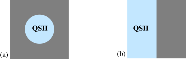
Figure 3: (a) Quantum spin Hall droplet immersed in the reference vacuum [in real space $(x,y)\in\mathbb{R}^{2}$]. (b) The $\mathbb{Z}^{\ }_{2}$ network model or its tight-binding equivalent when $x<0$ is separated from the reference vacuum at $x>0$ by the vertical boundary $x=0$ [in real space $(x,y)\in\mathbb{R}^{2}$].

The value (9fp) taken by the SU(2) Wilson loop thus appears to be ambiguous since it depends on the sign of the mass $m$. This ambiguity is a mere reflection of the fact that, as noted in [20], the topological nature of the $\mathbb{Z}^{\ }_{2}$ network model is itself defined relative to that of some reference vacuum. Indeed, for any given choice of the parameters $(X,\theta)$ from figure 2 that defines uniquely the bulk properties of the insulating phase in the $\mathbb{Z}^{\ }_{2}$ network model, the choice of boundary conditions determines if a single helical Kramers’ doublet edge state is or is not present at the boundary of the $\mathbb{Z}^{\ }_{2}$ network model. In view of this, it is useful to reinterpret the $\mathbb{Z}^{\ }_{2}$ network model with a boundary as realizing a quantum spin Hall droplet immersed in a reference vacuum as is depicted in figure 3(a). If so, choosing the boundary condition is equivalent to fixing the topological attribute of the reference vacuum relative to that of the $\mathbb{Z}^{\ }_{2}$ network model, for the reference vacuum in which the quantum spin Hall droplet is immersed also has either a trivial or non-trivial $\mathbb{Z}^{\ }_{2}$ quantum topology. A single helical Kramers’ doublet propagating unhindered along the boundary between the quantum spin Hall droplet and the reference vacuum appears if and only if the $\mathbb{Z}^{\ }_{2}$ topological quantum numbers in the droplet and in the reference vacuum differ.

In the low-energy continuum limit (9dm), a boundary in real space can be introduced by breaking translation invariance along the vertical line $x=0$ in the real space $(x,y)\in\mathbb{R}^{2}$ through the profile [see figure 3(b)]

$$m(x,y)=m(x)=\left\{\begin{array}[]{cc}-m,&\hbox{if $x\to-\infty$,}\\ &\\ +m,&\hbox{if $x\to+\infty$,}\end{array}\right.$$ (9fq)

for the mass.

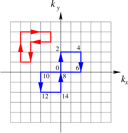
Figure 4: Momentum space $(k^{\ }_{x},k^{\ }_{y})\in\mathbb{R}^{2}$ is discretized with the help of a rectangular grid on which two paths are depicted. The red path that is restricted to the upper left quadrant is not invariant as a set under the inversion $(k^{\ }_{x},k^{\ }_{y})\to-(k^{\ }_{x},k^{\ }_{y})$. The blue path with its center of mass at the origin is. This path is assembled out of 16 links: $(i^{\ }_{0},i^{\ }_{1})=-(i^{\ }_{15},i^{\ }_{0})$, $(i^{\ }_{1},i^{\ }_{2})=-(i^{\ }_{14},i^{\ }_{15})$, $(i^{\ }_{2},i^{\ }_{3})=-(i^{\ }_{13},i^{\ }_{14})$, $(i^{\ }_{3},i^{\ }_{4})=-(i^{\ }_{12},i^{\ }_{13})$, $(i^{\ }_{4},i^{\ }_{5})=-(i^{\ }_{11},i^{\ }_{12})$, $(i^{\ }_{5},i^{\ }_{6})=-(i^{\ }_{10},i^{\ }_{11})$, $(i^{\ }_{6},i^{\ }_{7})=-(i^{\ }_{9},i^{\ }_{10})$, $(i^{\ }_{7},i^{\ }_{8})=-(i^{\ }_{8},i^{\ }_{9})$. Sites $i^{\ }_{0}=i^{\ }_{8}=i^{\ }_{16}$ along the path are the only ones invariant under $(k^{\ }_{x},k^{\ }_{y})\to-(k^{\ }_{x},k^{\ }_{y})$.

We close Sec. 3 with a justification of the master formula (9ek). To this end, we regularize the continuum gauge theory by discretizing momentum space (figure 4). We use the momentum coordinate $i\in\mathbb{Z}^{2}$ on a rectangular grid with the two lattice spacings $\Delta k^{\mu}>0$. To each link from the site $i$ to the nearest-neighbor site $i+\mu$ of the grid, we assign the SU(2) unitary matrix

$$U^{\ }_{i,i+\mu}\equiv\rme^{A^{\ }_{i,i+\mu}\Delta k^{\mu}},$$ (9fr)

which is obtained by discarding U(1) part of the U(2) Berry connection. Consistency demands that

$$U^{\ }_{i+\mu,i}=U^{{\dagger}}_{i,i+\mu}\Longleftrightarrow A^{\ }_{i+\mu,i}=A^{{\dagger}}_{i,i+\mu}.$$ (9fs)

We define the SU(2) Wilson loop to be

$$W^{\ }_{\mathrm{SU}(2)}(i^{\ }_{0},\cdots,i^{\ }_{N-1}):=\frac{1}{2}\mathrm{tr}\!\left(U^{\ }_{i^{\ }_{0},i^{\ }_{1}}U^{\ }_{i^{\ }_{1},i^{\ }_{2}}\cdots U^{\ }_{i^{\ }_{N-1},i^{\ }_{0}}\right)$$ (9ft)

where $i^{\ }_{n}$ and $i^{\ }_{n+1}$ are nearest neighbors, i.e., their difference $i^{\ }_{n+1}-i^{\ }_{n}=\eta^{\ }_{n}$ is a unit vector $\eta^{\ }_{n}$. The Wilson loop is invariant under any local gauge transformation by which

$$U^{\ }_{i,i+\mu}\to V^{{\dagger}}_{i}U^{\ }_{i,i+\mu}V^{\ }_{i+\mu}$$ (9fu)

where the $V^{\vphantom{i}}_{i}$’s are U(2) matrices. Observe that the cyclicity of the trace allows us to write

$$W^{\ }_{\mathrm{SU}(2)}(i^{\ }_{0},\cdots,i^{\ }_{N-1})=\frac{1}{2}\mathrm{tr}\!\left(U^{\ }_{i^{\ }_{\frac{N}{2}},i^{\ }_{\frac{N}{2}+1}}\cdots U^{\ }_{i^{\ }_{N-1},i^{\ }_{0}}U^{\ }_{i^{\ }_{0},i^{\ }_{1}}U^{\ }_{i^{\ }_{1},i^{\ }_{2}}\cdots U^{\ }_{i^{\ }_{\frac{N}{2}-1},i^{\ }_{\frac{N}{2}}}\right).$$ (9fv)

To make contact with the master formula (9ek), we assume that the closed path with vertices $i^{\ }_{\ell}$ parametrized by the index $\ell=0,1,\cdots,N-1$ obeys the condition that

$$\vdots$$

$$\mbox{$i^{\ }_{N-n}$ is the wave vector $-\sum_{m=1}^{n}\eta^{\ }_{m}\Delta k^{\mu^{\ }_{m}}$},$$

$$\vdots$$

$$\mbox{$i^{\ }_{N-1}$ is the wave vector $-\eta^{\ }_{1}\Delta k^{\mu^{\ }_{1}}$},$$

$$\mbox{$i^{\ }_{0}$ is the wave vector $0$},$$ (9fw)

$$\mbox{$i^{\ }_{1}$ is the wave vector $+\eta^{\ }_{1}\Delta k^{\mu^{\ }_{1}}$},$$

$$\vdots$$

$$\mbox{$i^{\ }_{n}$ is the wave vector $+\sum_{m=1}^{n}\eta^{\ }_{m}\Delta k^{\mu^{\ }_{m}}$},$$

$$\vdots$$

with $\eta^{\ }_{m}=\pm 1$ for $m=1,\cdots,N/2$ in order to mimic after discretization the condition that the closed path entering the Wilson loop is invariant as a set under the inversion (9ei).

On the discretized momentum lattice the sewing matrix (9dp) is defined by

$$\bigl{(}w^{\ }_{i}\bigr{)}_{\hat{a}\hat{b}}:=\langle u^{\ }_{\hat{a}}(-i)|\hat{\Theta}|u^{\ }_{\hat{b}}(i)\rangle,$$ (9fx)

which obeys the condition

$$w^{\ }_{-i}=-w^{\mathrm{T}}_{i},$$ (9fy)

i.e., the counterpart to the relation (9dq). This implies that $w^{\ }_{i^{\ }_{0}}$ and $w^{\ }_{i^{\ }_{N/2}}$ are antisymmetric unitary $2\times 2$ matrices. Furthermore, the sewing matrix $w^{\ }_{i}$ must also obey the counterpart to (9dz), namely

$$U^{\ }_{-j,-i}=w^{\ }_{j}U^{\mathrm{T}}_{i,j}w^{{\dagger}}_{i}.$$ (9fz)

It now follows from (9fw) and (9fz) that

$$U^{\ }_{i^{\ }_{N-1},i^{\ }_{0}}=w^{\ }_{i^{\ }_{1}}U^{\mathrm{T}}_{i^{\ }_{0},i^{\ }_{1}}w^{{\dagger}}_{i^{\ }_{0}},$$

$$\vdots$$

$$U^{\ }_{i^{\ }_{N-1-n},i^{\ }_{N-n}}=w^{\ }_{i^{\ }_{n+1}}U^{\mathrm{T}}_{i^{\ }_{n},i^{\ }_{n+1}}w^{{\dagger}}_{i^{\ }_{n}},$$ (9ga)

$$\vdots$$

$$U^{\ }_{i^{\ }_{\frac{N}{2}},i^{\ }_{\frac{N}{2}+1}}=w^{\ }_{i^{\ }_{\frac{N}{2}}}U^{\mathrm{T}}_{i^{\ }_{\frac{N}{2}-1},i^{\ }_{\frac{N}{2}}}w^{{\dagger}}_{i^{\ }_{\frac{N}{2}-1}}.$$

In particular, we observe that

$$U^{\ }_{i^{\ }_{N-1},i^{\ }_{0}}U^{\ }_{i^{\ }_{0},i^{\ }_{1}}=w^{\ }_{i^{\ }_{1}}U^{\mathrm{T}}_{i^{\ }_{0},i^{\ }_{1}}w^{{\dagger}}_{i^{\ }_{0}}U^{\ }_{i^{\ }_{0},i^{\ }_{1}}=w^{\ }_{i^{\ }_{1}}w^{{\dagger}}_{i^{\ }_{0}}U^{{\dagger}}_{i^{\ }_{0},i^{\ }_{1}}U^{\ }_{i^{\ }_{0},i^{\ }_{1}}=w^{\ }_{i^{\ }_{1}}w^{{\dagger}}_{i^{\ }_{0}},$$ (9gb)

since $w^{\ }_{i^{\ }_{0}}$ is a $2\times 2$ antisymmetric unitary matrix, i.e., $w^{\ }_{i^{\ }_{0}}$ is the second Pauli matrix up to a phase factor, while

$$(\bm{\rho}\cdot\bm{n})^{\mathrm{T}}\rho^{\ }_{2}=-\rho^{\ }_{2}(\bm{\rho}\cdot\bm{n})$$ (9gc)

holds for any three-vector $\bm{n}$ contracted with the three-vector $\bm{\rho}$ made of the three Pauli matrices. By repeating the same exercise a second time,

$$U^{\ }_{i^{\ }_{N-2},i^{\ }_{N-1}}\left(U^{\ }_{i^{\ }_{N-1},i^{\ }_{0}}U^{\ }_{i^{\ }_{0},i^{\ }_{1}}\right)U^{\ }_{i^{\ }_{1},i^{\ }_{2}} =w^{\ }_{i^{\ }_{2}}U^{\mathrm{T}}_{i^{\ }_{1},i^{\ }_{2}}w^{{\dagger}}_{i^{\ }_{1}}\left(w^{\ }_{i^{\ }_{1}}w^{{\dagger}}_{i^{\ }_{0}}\right)U^{\ }_{i^{\ }_{1},i^{\ }_{2}}$$ (9gd)

$$=w^{\ }_{i^{\ }_{2}}w^{{\dagger}}_{i^{\ }_{0}},$$

one convinces oneself that the dependences on the gauge fields $A^{\ }_{i^{\ }_{0},i^{\ }_{1}}$ and $A^{\ }_{i^{\ }_{N-1},i^{\ }_{0}}$, $A^{\ }_{i^{\ }_{1},i^{\ }_{2}}$ and $A^{\ }_{i^{\ }_{N-2},i^{\ }_{N-1}}$, and so on until $A^{\ }_{i^{\ }_{n-1},i^{\ }_{n}}$ and $A^{\ }_{i^{\ }_{N-n},i^{\ }_{N-n+1}}$ at the level $n$ of this iteration cancel pairwise due to the conditions (9fw)–(9fz) implementing time-reversal invariance. This iteration stops when $n=N/2$, in which case the SU(2) Wilson loop is indeed solely controlled by the sewing matrix at the time-reversal invariant momenta corresponding to $\ell=0$ and $\ell=N/2$,

$$W^{\ }_{\mathrm{SU}(2)}(i^{\ }_{0},\cdots,i^{\ }_{N-1})=\frac{1}{2}\mathrm{tr}\!\left(w^{\ }_{i^{\ }_{N/2}}w^{{\dagger}}_{i^{\ }_{0}}\right).$$ (9ge)

Since $i^{\ }_{0}$ and $i^{\ }_{N/2}$ are invariant under momentum inversion or, equivalently, time-reversal invariant,

$$w^{\ }_{i^{\ }_{N/2}}=\rme^{\mathrm{i}\alpha^{\ }_{N/2}}\,\rmi\rho^{\ }_{2},\qquad w^{\ }_{i^{\ }_{0}}=\rme^{\mathrm{i}\alpha^{\ }_{0}}\,\rmi\rho^{\ }_{2}$$ (9gf)

with $\alpha^{\ }_{N/2},\alpha^{\ }_{0}=0,\pi$. Here, the $\mathbb{Z}^{\ }_{2}$ phases $\rme^{\mathrm{i}\alpha^{\ }_{N/2}}$ and $\rme^{\mathrm{i}\alpha^{\ }_{0}}$ are none other than the Pfaffians

$$\rme^{\mathrm{i}\alpha^{\ }_{N/2}}=\mathrm{Pf}\!\left(w^{\ }_{i^{\ }_{N/2}}\right),\qquad\rme^{\mathrm{i}\alpha^{\ }_{0}}=\mathrm{Pf}\!\left(w^{\ }_{i^{\ }_{0}}\right),$$ (9gg)

respectively. Hence,

$$W^{\ }_{\mathrm{SU}(2)}(i^{\ }_{0},\cdots,i^{\ }_{N-1}) =\frac{1}{2}\mathrm{tr}\!\left[\mathrm{Pf}\!\left(w^{\ }_{i^{\ }_{N/2}}\right)\mathrm{i}\rho^{\ }_{2}\times\mathrm{Pf}\!\left(w^{{\dagger}}_{i^{\ }_{0}}\right)(-\rmi\rho^{\ }_{2})\right]$$ (9gh)

$$=\mathrm{Pf}\!\left(w^{\ }_{i^{\ }_{N/2}}\right)\mathrm{Pf}\!\left(w^{\ }_{i^{\ }_{0}}\right)$$

is a special case of (9ek). (Recall that $w^{\ }_{i^{\ }_{0}}$ and $w^{\ }_{i^{\ }_{N/2}}$ are real-valued.)

4 Numerical study of boundary multifractality in the $\mathbb{Z}^{\ }_{2}$ network model

In [20], we have shown that (i) multifractal scaling holds near the boundary of the $\mathbb{Z}^{\ }_{2}$ network model at the transition between the metallic phase and the $\mathbb{Z}^{\ }_{2}$ topological insulating phase shown in figure 2, (ii) it is different from that in the ordinary symplectic class, while (iii) bulk properties, such as the critical exponents for the divergence of the localization length and multifractal scaling in the bulk, are the same as those in the conventional two-dimensional symplectic universality class of Anderson localization. This implies that the boundary critical properties are affected by the presence of the helical edge states in the topological insulating phase adjacent to the critical point. In this work, we improve the precision for the estimate of the boundary multifractal critical exponents. We also compute numerically additional critical exponents that encode corner (zero-dimensional) multifractality at the metal-to-$\mathbb{Z}^{\ }_{2}$-topological-insulator transition. We thereby support the claim that conformal invariance is present at the metal-to-$\mathbb{Z}^{\ }_{2}$-topological-insulator transition by verifying that conformal relations between critical exponents at these boundaries hold.

4.1 Boundary and corner multifractality

To characterize multifractal scaling at the metal-insulator transition in the $\mathbb{Z}^{\ }_{2}$ network model, we start from the time-evolution of the plane waves along the links of the network with the scattering matrices defined in (1)-(7) at the nodes $\mathsf{S}$ and $\mathsf{S}^{\prime}$. To minimize finite size effects, the parameter $\theta$ in (1)-(7) is chosen to be a random variable as explained in Sec. 2. We focus on the metal-insulator transition at $X=X^{\ }_{l}=0.971$ as shown in figure 2(b).

When we impose reflecting boundary conditions, a node on the boundary reduces to a unit $2\times 2$ matrix. When the horizontal reflecting boundaries are located at nodes of type $\mathsf{S}^{\prime}$, as shown in figure 5(a), there exists a single helical edge states for $X>X^{\ }_{l}$. The insulating phase $X>X^{\ }_{l}$ is thus topologically nontrivial.

For each realization of the disorder, we numerically diagonalize the one-step time-evolution operator of the $\mathbb{Z}^{\ }_{2}$ network model and retain the normalized wave function $\psi^{\ }_{\sigma}(x,y)$, after coarse graining over the 4 edges of the plaquette located at $(x,y)$, whose eigenvalue is the closest to $1$. The wave function at criticality is observed to display the power-law dependence on the linear dimension $L$ of the system,

$$\sum_{\sigma=\uparrow,\downarrow}|\psi^{\ }_{\sigma}(x,y)|^{2q}\propto L^{-\Delta^{(\zeta,\nu)}_{q}-dq}.$$ (9gi)

The anomalous dimension $\Delta^{(\zeta,\nu)}_{q}$, if it displays a nonlinear dependence on $q$, is the signature of multifractal scaling. The index $\zeta$ indicates whether the multifractal scaling applies to the bulk $(\zeta=2)$, the one-dimensional boundary $(\zeta=1)$, or to the zero-dimensional boundary (corner) $(\zeta=0)$, provided the plaquette $(x,y)$ is restricted to the corresponding regions of the $\mathbb{Z}^{\ }_{2}$ network model. For $\zeta=1$ and $0$, the index $\nu$ distinguishes the case $\nu=\mathrm{O}$ when the $\zeta$-dimensional boundary has no edge states in the insulating phase adjacent to the critical point, from the case $\nu=\mathbb{Z}^{\ }_{2}$ when the $\zeta$-dimensional boundary has helical edge states in the adjacent insulating phase. We ignore this distinction for multifractal scaling of the bulk wave functions, $\Delta^{(2,\mathrm{O})}_{q}=\Delta^{(2,\mathbb{Z}^{\ }_{2})}_{q}=\Delta^{(2)}_{q}$, since bulk properties are insensitive to boundary effects. We will also consider the case of mixed boundary condition for which we reserve the notation $\nu=\mathbb{Z}^{\ }_{2}|\mathrm{O}$.

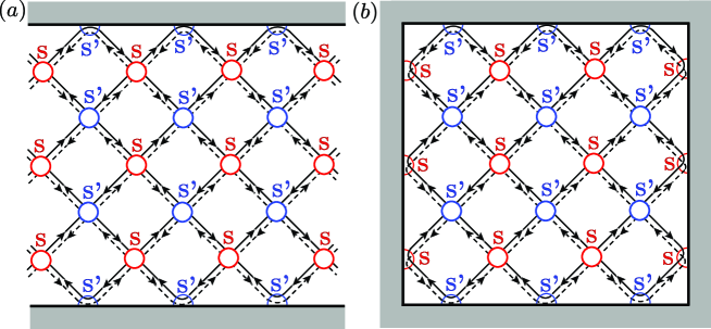
Figure 5: (a) Boundary multifractality is calculated from the wave function amplitudes near a one-dimensional boundary. Periodic (reflecting) boundary conditions are imposed for the horizontal (vertical) boundaries. (b) Corner multifractality is calculated from the wave function amplitudes near a corner with the wedge angle $\vartheta=\pi/2$. Reflecting boundary conditions are imposed along both vertical and horizontal directions. The relationship between the scattering matrix at a node of type $\mathsf{S}^{\prime}$ and the scattering matrix at a node of type $\mathsf{S}$ implies that it is a vertical boundary located at nodes of type $\mathsf{S}$ that induces an helical edge state when $X>X^{\ }_{l}$.

It was shown in [31] that boundary multifractality is related to corner multifractality if it is assumed that conformal invariance holds at the metal-insulator transition in the two-dimensional symplectic universality class. Conversely, the numerical verification of this relationship between boundary and corner multifractality supports the claim that the critical scaling behavior at this metal-insulator transition is conformal. So we want to verify numerically if the consequence of the conformal map $w=z^{\vartheta/\pi}$, namely

$$\Delta^{(0,\nu)}_{q}=\frac{\pi}{\vartheta}\Delta^{(1,\nu)}_{q}$$ (9gj)

where $\vartheta$ is the wedge angle at the corner, holds. Equivalently, $f^{(\zeta,\nu)}(\alpha)$, which is defined to be the Legendre transformation of $\Delta^{(\zeta,\nu)}_{q}+dq$, i.e.,

$$\alpha^{(\zeta,\nu)}_{q}=\frac{d\Delta^{(\zeta,\nu)}_{q}}{dq}+d,$$ (9gk)

$$f^{(\zeta,\nu)}(\alpha^{\ }_{q})=q\alpha^{(\zeta,\nu)}-\Delta^{(\zeta,\nu)}_{q}-dq+\zeta,$$ (9gl)

must obey

$$\alpha^{(0,\nu)}_{q}-d=\frac{\pi}{\vartheta}(\alpha^{(1,\nu)}_{q}-d),$$ (9gm)

$$f^{{(0,\nu)}}(\alpha)=\frac{\pi}{\vartheta}\!\left[f^{(1,\nu)}(\alpha)-1\right],$$ (9gn)

if conformal invariance is a property of the metal-insulator transition.

To verify numerically the formulas (9gj), (9gm), and (9gn), we consider the $\mathbb{Z}^{\ }_{2}$ network model with the geometries shown in figure 5. We have calculated wave functions for systems with the linear sizes $L=50,80,120,150,$ and $180$ for the two geometries displayed in figure 5. Here, $L$ counts the number of nodes of the same type along a boundary. The number of realizations of the static disorder is $10^{5}$ for each system size.

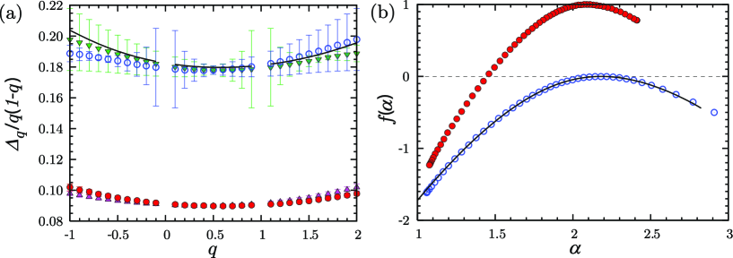
Figure 6: (a) The boundary (filled circles, red) and corner with $\theta=\pi/2$ (open circles, blue) anomalous dimensions at the metal-to-$\mathbb{Z}^{\ }_{2}$-topological-insulator transition. The solid curve is computed from (9gj) by using the boundary anomalous dimension as an input. The rescaled $\Delta^{\ }_{1-q}$ confirming the reciprocal relation for boundary and corner multifractality are shown by upper (magenta) and lower (green) triangles, respectively. (b) The multifractal spectra for the boundary (filled circles, red) and the corner (open circles, blue). The solid curve is computed from (9gm) and (9gn).

Figure 6(a) shows the boundary anomalous dimensions $\Delta^{(1,\mathbb{Z}^{\ }_{2})}_{q}$ (filled circles) and the corner anomalous dimensions $\Delta^{(0,\mathbb{Z}^{\ }_{2})}_{q}$ (open circles). In addition, the anomalous dimensions $\Delta^{(\zeta,\nu)}_{1-q}$ are shown by upper and lower triangles for boundary and corner anomalous dimensions, respectively. They fulfill the reciprocal relation

$$\Delta^{(\zeta,\nu)}_{q}=\Delta^{(\zeta,\nu)}_{1-q}$$ (9go)

derived analytically in [34]. Since the triangles and circles are consistent within error bars, our numerical results are reliable, especially between $0<q<1$. If we use the numerical values of $\Delta^{(1,\mathbb{Z}^{\ }_{2})}_{q}$ as inputs in (9gj) with $\vartheta=\pi/2$, there follows the corner multifractal scaling exponents that are plotted by the solid curve. Since the curve overlaps with the direct numerical computation of $\Delta^{(0,\mathbb{Z}^{\ }_{2})}_{q}$ within the error bars, we conclude that the relation (9gj) is valid at the metal-to-$\mathbb{Z}^{\ }_{2}$-topological-insulator transition.

Figure 6(b) shows the boundary (filled circles) and corner (open circles) multifractal spectra. These multifractal spectra are calculated by using (9gi), (9gk), and (9gl). The numerical values of $\alpha^{(\zeta,\mathbb{Z}^{\ }_{2})}_{0}$ are

$$\alpha^{(1,\mathbb{Z}^{\ }_{2})}_{0}=2.091\pm 0.002,$$ (9gp)

$$\alpha^{(0,\mathbb{Z}^{\ }_{2})}_{0}=2.179\pm 0.01.$$ (9gq)

The value of $\alpha^{(1,\mathbb{Z}^{\ }_{2})}_{0}$ is consistent with that reported in [20], while its accuracy is improved. The solid curve obtained from the relations (9gm) and (9gn) by using $f^{(1,\mathbb{Z}^{\ }_{2})}(\alpha)$ as an input, coincides with $f^{(0,\mathbb{Z}^{\ }_{2})}(\alpha)$. We conclude that the hypothesis of conformal invariance at the quantum critical point of metal-to-$\mathbb{Z}^{\ }_{2}$-topological-insulator transition is consistent with our numerical study of multifractal scaling.

At last, we would like to comment on the dependence on $z$ of

$$\langle\ln|\Psi|^{2}\rangle^{\ }_{z,L}\equiv\frac{1}{2L}\sum_{y=1}^{2L}\overline{\ln\left(\sum_{\sigma=\uparrow,\downarrow}|\psi^{\ }_{\sigma}(x,y)|^{2}\right)}$$ (9gr)

found in [20]. Here, $z\equiv(x-1)/2L$, while $x$ and $y$ denote the positions on the network along its axis and along its circumference, respectively (our choice of periodic boundary conditions imposes a cylindrical geometry). The overline denotes averaging over disorder. Figure 7(a) shows the $z$ dependence of $\langle\ln|\Psi|^{2}\rangle^{\ }_{z,L}$ for different values of $L$ in this cylindrical geometry at the metal-to-$\mathbb{Z}^{\ }_{2}$-topological-insulator transition. We observe that $\langle\ln|\Psi|^{2}\rangle^{\ }_{z,L}$ becomes a nonmonotonic function of $z$.

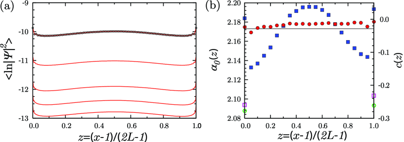
Figure 7: (a) The $z$ dependence of $\langle\ln|\Psi|^{2}\rangle^{\ }_{z,L}$ at the metal-to-$\mathbb{Z}^{\ }_{2}$-topological-insulator transition in the cylindrical geometry for $L=50,80,120,150,180$ from the top to the bottom. (b) The $z$ dependence of $\tilde{\alpha}^{\ }_{0}(z)$ (${\color[rgb]{1,0,0}\bullet}$)and $c(z)$ (${\color[rgb]{0,0,1}\blacksquare}$) extrapolated from the system size dependence of $\langle\ln|\Psi|^{2}\rangle^{\ }_{z,L}$ averaged over a small interval of $z$’s. $\tilde{\alpha}_{0}(z)$ and $c(z)$ at $z=0,1$ without averaging over a small interval of $z$’s are shown by open circles and squares, respectively. The solid line represents the bulk value of $\alpha^{(2)}_{0}=2.173$ computed in [31]. The asymmetry with respect to $z=0.5$ is due to statistical fluctuations.

We are going to argue that this nonmonotonic behavior is a finite size effect. We make the scaling ansatz

$$\langle\ln|\Psi|^{2}\rangle^{\ }_{z,L}=-\tilde{\alpha}^{(\zeta,\mathbb{Z}^{\ }_{2})}_{0}(z)\ln L+c(z),$$ (9gs)

where $\zeta=1$ if $z=0,1$ and $\zeta=2$ otherwise, while $c(z)$ depends on $z$ but not on $L$. To check the $L$ dependence of $\langle\ln|\Psi|^{2}\rangle^{\ }_{z,L}$ in figure 7, we average $\langle\ln|\Psi|^{2}\rangle^{\ }_{z,L}$ over a narrow interval of $z$’s for each $L$. Figure 7(b) shows the $z$ dependence of $\tilde{\alpha}^{\ }_{0}(z)$ ($\bullet$) and $c(z)$ ($\blacksquare$) obtained in this way. In addition, $\tilde{\alpha}^{\ }_{0}(z)$ and $c(z)$ calculated for $z=0,1$ without averaging over the narrow interval of $z$’s are shown by open circles and open squares, respectively.

We observe that $\tilde{\alpha}^{\ }_{0}(z)$, if calculated by averaging over a finite range of $z$’s, is almost constant and close to $\alpha^{(2)}_{0}=2.173$. In contrast, $\tilde{\alpha}^{\ }_{0}(z=0,1)\approx 2.09$, if calculated without averaging over a finite range of $z$’s, is close to $\alpha^{(1,\mathbb{Z}^{\ }_{2})}_{0}=2.091$. We also find that $|c(z)|$ increases near the boundaries. We conclude that it is the nonmonotonic dependence of $|c(z)|$ on $z$ that gives rise to the nonmonotonic dependence of $\langle\ln|\Psi|^{2}\rangle^{\ }_{z,L}$ on $z$. This finite-size effect is of order $1/\ln L$ and vanishes in the limit $L\to\infty$.

4.2 Boundary condition changing operator

Next, we impose mixed boundary conditions by either (i) coupling the $\mathbb{Z}^{\ }_{2}$ network model to an external reservoir through point contacts or (ii) by introducing a long-range lead between two nodes from the $\mathbb{Z}^{\ }_{2}$ network model, as shown in figure 8. In this way, when $X>X^{\ }_{l}$, a single Kramers’ pair of helical edge states indicated by the wavy lines in figure 8 is present on segments of the boundary, while the complementary segments of the boundary are devoid of any helical edge state (the straight lines in figure 8). The helical edge states either escape the $\mathbb{Z}^{\ }_{2}$ network model at the nodes at which leads to a reservoir are attached [the green lines in figure 8(a) and figure 8(b)], or shortcut a segment of the boundary through a nonlocal connection between the two nodes located at the corners [figure 8(c)]. These are the only options that accommodate mixed boundary conditions and are permitted by time-reversal symmetry. As shown by Cardy in [35], mixed boundary conditions are implemented by boundary-condition-changing operators in conformal field theory. Hence, the geometries of figure 8 offer yet another venue to test the hypothesis of two-dimensional conformal invariance at the metal-insulator quantum critical point.

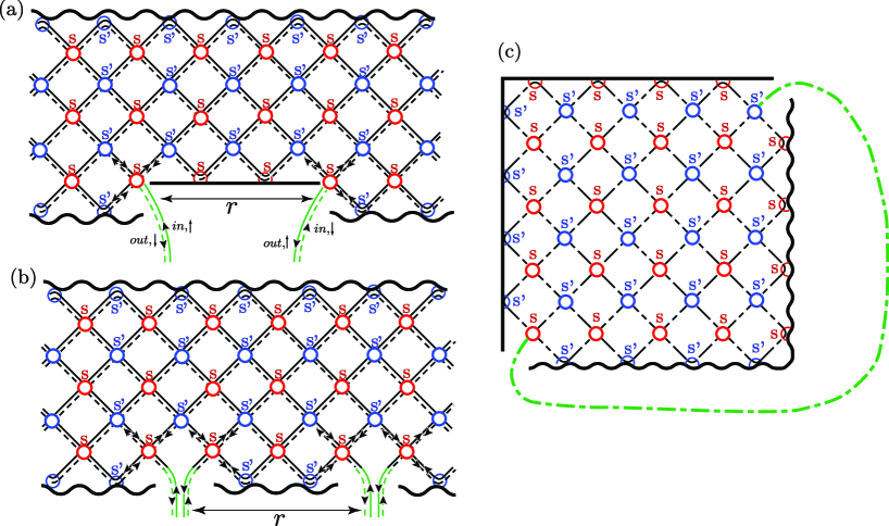
Figure 8: (a) The system with two point contacts (green curves) attached (a) at the two interfaces between different types of boundaries and (b) at the reflecting boundary. The periodic boundary conditions are imposed for the horizontal direction. The thick wavy and solid lines on the edges represent two different types of boundaries, with and without a helical edge mode at $X>X_{l}$, respectively. (c) Closed network with mixed boundaries. Each dashed line or curve represents a Kramers’ doublet.

When coupling the $\mathbb{Z}^{\ }_{2}$ network model to an external reservoir, we shall consider two cases shown in figure 8(a) and figure 8(b), respectively.

First, we consider the case of figure 8(a) in which only two nodes from the $\mathbb{Z}^{\ }_{2}$ network model couple to the reservoir. At each of these point contacts, the scattering matrix $S$ that relates incoming to outgoing waves from and to the reservoir is a $2\times 2$ matrix which is invariant under time reversal $s_{2}S^{*}s_{2}=S$, and it must be proportional to the unit $2\times 2$ matrix up to an overall (random) phase. Hence, the two-point-contact conductance in the geometry of figure 8(a) is unity, however far the two point contacts are from each other.

Second, we consider the case of figure 8(b) in which there are again two point contacts, however each lead between the $\mathbb{Z}^{\ }_{2}$ network model and the reservoir now supports two instead of one Kramers’ doublets. The two point-contact scattering matrices connecting the $\mathbb{Z}^{\ }_{2}$ network model to the reservoirs are now $4\times 4$ matrices, which leads to a non-vanishing probability of backscattering. Hence, this even channel two-point-contact conductance is expected to decay as a function of the separation between the two attachment points of the leads to the network.

To test whether the two-point-contact conductance in figure 8(a) and figure 8(b) do differ as dramatically as anticipated, we have computed numerically the two-point-contact conductance at the quantum critical point $X=X^{\ }_{l}$ for a single realization of the static disorder. The two-point-contact conductance is calculated by solving for the stationary solution of the time-evolution operator with input and output leads [36]. We choose the cylindrical geometry imposed by periodic boundary conditions along the horizontal directions in figures 8(a) and 8(b) for a squared network with the linear size $L=200$. Figure 9(a) shows with the symbol $\bullet$ the dependence on $r$, the distance between the two contacts in figure 8(a), of the dimensionless two-point-contact conductance $g$. It is evidently $r$ independent and unity, as expected. Figure 9(a) also shows with the symbol $\circ$ the dependence on $r$ of the dimensionless two-point conductance $g$ for leads supporting two Kramers’ doublet as depicted in figure 8(b). Although it is not possible to establish a monotonous decay of the two-point-contact conductance for a single realization of the static disorder, its strong fluctuations as $r$ is varied are consistent with this claim.

We turn our attention to the closed geometry shown in figure 8(c). We recall that it is expected on general grounds that the moments of the two-point conductance in a network model at criticality, when the point contacts are far apart, decay as power laws with scaling exponents proportional to the scaling exponents $\Delta^{(\zeta,\nu)}_{q}$ [36, 37]. Consequently, after tuning the $\mathbb{Z}^{\ }_{2}$ network model to criticality, the anomalous dimensions at the node (corner) where the boundary condition is changed must vanish,

$$\Delta^{(0,\mathbb{Z}^{\ }_{2}|\mathrm{O})}_{q}=0,$$ (9gt)

since the two-point-contact conductance in figure 8(a) is $r$ independent. (9gt) is another signature of the nontrivial topological nature of the insulating side at the Anderson transition that we want to test numerically. Thus, we consider the geometry figure 8(c) and compute numerically the corner anomalous dimensions. This is done using the amplitudes of the stationary wave function restricted to the links connecting the two corners where the boundary conditions are changed. Figure 9(b) shows the numerical value of the corner anomalous dimension $\Delta^{(0,\mathbb{Z}^{\ }_{2}|\mathrm{O})}_{q}$. The linear sizes of the network are $L=50,80,120,150$, and $180$ and the number of disorder realizations is $10^{5}$ for each $L$. We observe that $\Delta^{(0,\mathbb{Z}^{\ }_{2}|\mathrm{O})}_{q}$ is zero within the error bars, thereby confirming the validity of the prediction (9gt) at the metal-to-$\mathbb{Z}^{\ }_{2}$-topological-insulator transition.

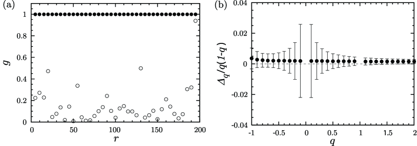
Figure 9: (a) The distance $r$ dependence of the two-point-contact conductance $g$ for the mixed boundary ($\bullet$) and the reflecting boundary ($\circ$). (b) The zero dimensional anomalous dimension $\Delta^{(0,\mathbb{Z}^{\ }_{2}|\mathrm{O})}_{q}$ obtained from the wave function amplitude on the link which connecting the boundary condition changing points.

5 Conclusions

In summary, we have mapped the $\mathbb{Z}^{\ }_{2}$ network model to a $4\times 4$ Dirac Hamiltonian. In the clean limit of this Dirac Hamiltonian, we expressed the Kane-Mele $\mathbb{Z}^{\ }_{2}$ invariant as an SU(2) Wilson loop and computed it explicitly. In the presence of weak time-reversal symmetric disorder, the NLSM that can be derived out of this Dirac Hamiltonian describes the metal-insulator transition in the $\mathbb{Z}^{\ }_{2}$ network model and yields bulk scaling exponents that belong to the standard two-dimensional symplectic universality class; an expectation confirmed by the numerics in [19] and [20]. A sensitivity to the $\mathbb{Z}^{\ }_{2}$ topological nature of the insulating state can only be found by probing the boundaries, which we did numerically in the $\mathbb{Z}^{\ }_{2}$ network model by improving the quality of the numerical study of the boundary multifractality in the $\mathbb{Z}^{\ }_{2}$ network model.

References

References

- [1] Roland Winkler 2003 “Spin-orbit coupling effects in two-dimensional electron and hole systems,” (Springer-Verlag Berlin Heidelberg)
- [2] Hikami S, Larkin A I and Nagaoka Y 1980 Prog. Theor. Phys. 63 707
- [3] Kane C L and Mele E J 2005 Phys. Rev. Lett. 95 226801
- [4] Kane C L and Mele E J 2005 Phys. Rev. Lett. 95 146802
- [5] Bernevig B A and Zhang S C 2006 Phys. Rev. Lett. 96 106802
- [6] Bernevig B A, Hughes T L and Zhang S C 2006 Science 314 1757
- [7] König M, Wiedmann S, Brüne C, Roth A, Buhmann H, Molenkamp L W, Qi X L and Zhang S C 2007 Science 318 766
- [8] Moore J E and Balents L 2007 Phys. Rev. B 75 121306(R)
- [9] Roy R 2009 Phys. Rev. B 79 195322
- [10] Fu L, Kane C L and Mele E J 2007 Phys. Rev. Lett. 98 106803
- [11] Hsieh D, Qian D, Wray L, Xia Y, Hor Y, Cava R and Hasan M Z 2008 Nature 452 970
- [12] Hsieh D, Xia Y, Wray L, Qian D, Pal A, Dil J H, Osterwalder J, Meier R, Bihknayer G, Kane C L, Hor Y, Cava R, and Hasan M 2009 Science 323 919
- [13] Xia Y, Qian D, Hsieh D, Wray L, Pal A, Lin H, Bansil A, Grauer D, Hor Y S, Cava R J, and Hasan M Z 2009 Nature Phys. 5 398
- [14] Hsieh D, Xia Y, Qian D, Wray L, Dil J H, Meier F, Osterwalder J, Patthey L, Checkelsky J G, Ong N P, Fedorov A V, Lin H, Bansil A, Grauer D, Hor Y S, Cava R J, and Hasan M Z 2009 Nature 460 1101
- [15] Chen Y L, Analytis J G, Chu J-H, Liu Z K, Mo S-K, Qi X L, Zhang H J, Lu D H, Dai X, Fang Z, Zhang S C, Fisher I R, Hussain Z, and Shen Z-X 2009 Science 325 178
- [16] Thouless D J, Kohmoto M, Nightingale M P and den Nijs M 1982 Phys. Rev. Lett. 49 405
- [17] Fu L and Kane C L 2006 Phys. Rev. B 74 195312
- [18] Onoda M, Avishai Y and Nagaosa N 2007 Phys. Rev. Lett. 98 076802
- [19] Obuse H, Furusaki A, Ryu S and Mudry C 2007 Phys. Rev. B. 76 075301
- [20] Obuse H, Furusaki A, Ryu S and Mudry C 2008 Phys. Rev. B. 78 115301
- [21] Chalker J T and Coddington P D 1988 J. Phys. C 21 2665
- [22] Kramer B, Ohtsuki T and Kettemann S 2005 Phys. Rep. 417 211
- [23] Wegner F J 1979 Z. Phys. B 35 207
- [24] Fendley P 2001 Phys. Rev. B 63 104429
- [25] Ryu S, Mudry S, Obuse H and Furusaki A 2007 Phys. Rev. Lett. 99 116601
- [26] Ostrovsky P M, Gornyi I V and Mirlin A D 2007 Phys. Rev. Lett. 98 256801
- [27] Bardarson J H, Tworzydło J, Brouwer P W, and Beenakker C W J, Phys. Rev. Lett. 99, 106801 (2007).
- [28] Nomura K, Koshino M, and Ryu S 2007 Phys. Rev. Lett. 99 146806
- [29] Schnyder A P, Ryu S, Furusaki A and Ludwig A W W 2008 Phys. Rev. B 78 195125
- [30] Subramaniam A R, Gruzberg I A, Ludwig A W W, Evers F, Mildenberger A and Mirlin A D 2006 Phys. Rev. Lett. 96 126802
- [31] Obuse H, Subramaniam A R, Furusaki A, Gruzberg I A and Ludwig A W W 2007 Phys. Rev. Lett. 98 156802
- [32] Ho C M and Chalker J T 1996 Phys. Rev. B 54 8708
- [33] Ludwig A W W, Fisher M P A, Shankar R and Grinstein G 1994 Phys. Rev. B 50 7526
- [34] Mirlin A D, Fyodorov Y V, Mildenberger A and Evers F 2006 Phys. Rev. Lett. 97 046803
- [35] Cardy J L 1989 Nucl. Phys. B 324 581
- [36] Janssen M, Metzler M and Zirnbauer M R 1999 Phys. Rev. B 59 15836
- [37] Klesse R and Zirnbauer M R 2001 Phys. Rev. Lett. 86 2094