The role of multigrid algorithms for LQCD

Abstract:

We report on the first successful QCD multigrid algorithm which demonstrates constant convergence rates independent of quark mass and lattice volume for the Wilson Dirac operator. The new ingredient is the adaptive method for constructing the near null space on which the coarse grid multigrid Dirac operator acts. In addition we speculate on future prospects for extending this algorithm to the Domain Wall and Staggered discretizations, its exceptional suitability for high performance GPU code and its potential impact on simulations at the physical pion mass.

1 Introduction

Perhaps the most severe computational challenge facing lattice Quantum Chromodynamics is the divergent cost as one approaches the chiral limit required for the experimental value of the pion mass. Similar difficulties confront other strongly-coupled field theories conjectured for physics beyond the standard model. The cause is well known. As the quark mass, $m_{q}$, approaches zero, the lattice Dirac operator becomes singular, $|\lambda_{min}|\;\rightarrow 0$, causing “critical slowing down” of the iterative solvers typically used to find the propagators. This is unavoidable for all local “unigrid” solvers.

It has been almost 20 years since the first attempts [1] were made to apply recursive multigrid preconditioning to the Dirac operator in lattice QCD. The basic idea of using a coarse representation of the Dirac operator on lattices of increasing lattice spacing appears at first to be an obvious extension of the basic principles central to the renormalization group itself. Indeed early attempts, generally inspired by this observation, did succeed in formulating a variety of gauge invariant coarsening schemes but they all failed to improve convergence at the length scale $l_{\sigma}$, where the underlying lattice gauge field becomes rough. Indeed as Brower, Edwards, Rebbi and Vicari [2] demonstrated this failure occurred uniformly when the product of the mass gap $m_{q}$ and the coherence length $l_{\sigma}$ is of order one: $m_{q}l_{\sigma}=O(1)$. Apparently this failure occurs when the “renormalization” is highly non-perturbative.

Recently the application of a new adaptive procedure [3] has decisively broken this barrier eliminating “critical slowing down” as the mass gap goes to zero [4]. Here we give a heuristic introduction to this breakthrough and speculate on further developments.

2 Adaptive Multigrid

While the detailed design of an appropriate adaptive multigrid algorithm for QCD requires considerable effort as reported in Ref. [4] the underlying concept is rather straightforward. We seek to accelerate the solver for a differential operator discretized on a hypercubic lattice with spacing $a$

$$D_{xy}\psi_{y}=b_{x}\;,$$ (1)

by preconditioning it with a coarse operator $\hat{D}$ at a larger lattice spacing $\hat{a}>a$. To be concrete our example is the Wilson lattice Dirac operator,

$$D_{xy}(U)=(4+m)\delta_{xy}+\sum^{4}_{\mu=1}[\frac{\gamma_{\mu}-1}{2}U_{\mu}(x)\delta_{x,y+\mu}-\frac{\gamma_{\mu}+1}{2}U^{\dagger}_{\mu}(x)\delta_{x+\mu,y}]\;,$$ (2)

where we have suppressed the indices for the 3x3 (dense) SU(3) color matrices $U^{ab}_{\mu}(x)$ and the 4x4 (sparse) spinor matrices $\gamma^{ij}_{\mu}$ in the tensor product. The fine Dirac matrix, $D$, operates on a complex vector space $V$ of dimension $12L^{3}\times T$.

Critical slowing down is caused by eigenvectors with small eigenvalues. This offending subspace is the near null space of our operator: $D:S\simeq 0$. Multigrid methods require us to split the fine vectors space $V$ into this near null space $S$ and its orthogonal complement $S_{\perp}$: $V=S+S_{\perp}$, in the language of the renormalization group, splitting the IR (near null) from the UV (rough) modes. One may view this splitting as a generalization of red/black or Schwartz block decompositions and the resultant preconditioning matrix as akin to using the Schur compliment. This splitting is achieved by a non-square prolongation matrix $P$ which maps the coarse space into the near null space S,

$$P:\hat{V}\rightarrow S\;,$$ (3)

as illustrated in Fig 1.

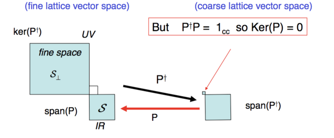
Figure 1: The non-square prolongation matrix P with $ker(P)=0$ defines a one to one map $P:\hat{V}=S$ from the coarse vector space $\hat{V}$ into the near null subspace $S$ of the fine vector space: $V=S+S_{\perp}$. The fundamental theorem of linear algebra gives $S=span(P)$, $\hat{V}=span(P^{\dagger})$ and $rank(P)=rank(P^{\dagger})=dim(S)$.

Then the multigrid cycle constructs a coarse matrix, $\hat{D}=RDP$, as the product of the prolongator ($P$) to the near null space on the fine lattice, the fine operator ($D$) and a restriction operator ($R$) back to the coarse lattice. We use the Galerkin form by setting $R=P^{\dagger}$.

To understand intuitively how one constructs this mapping, consider multigrid for the classic example of a d-dimensional discretized Laplace operator. The near null eigenvectors are literally smooth, dominated by low Fourier components. An obvious interpolation consists of piecewise constant functions on regular blocks to define the coarse degrees of freedom. For example on each $4^{d}$ block labeled by $\hat{x}$ we many introduce the prolongator (or interpolating matrix),

$$P_{x\hat{x}}=\frac{\theta_{\hat{x}}(x)}{2^{d}}\quad,\quad\theta_{\hat{x}}(x)=\left\{\begin{array}[]{ll}1&x\in\hat{x}\;\mbox{block}\\ 0&x\in\!\!\!\!\!\!\!/\;\;\hat{x}\;\mbox{block}\end{array}\right.\;,$$ (4)

where the blocking “theta function” , $\theta_{\hat{x}}(x)$, is 1 (true) for x inside and 0 (false) outside the block $\hat{x}$. The normalization is chosen so that $[P^{\dagger}P]_{\hat{x}\hat{y}}=\delta_{\hat{x},\hat{y}}$. The span of this space consists of all linear combinations of these basis vectors: $\psi_{x}=\sum_{\hat{x}}c_{\hat{x}}P_{x\hat{x}}$. Solving the coarse problem exactly for the error would reduce the residue to $r^{\prime}={\cal P}r=(1-DP\frac{1}{P^{\dagger}DP}P^{\dagger})r$, where

$${\cal P}=1-DP\frac{1}{P^{\dagger}DP}P^{\dagger}\quad,\quad{\cal P}^{2}={\cal P}$$ (5)

is the Petrov-Galerkin (oblique) projection operator with eigenvalues 0 and 1. This projector completely removes the near null space from the residue: $P{\cal P}=0$ but the transverse space $S_{\perp}$ of rough modes are left intact. To damp them out a smoother on the fine lattice must also be applied.

Fortunately this basic construction carriers over to the non-trivial example of lattice QCD. However to construct a parameterization for the coarse lattice Dirac operator, a piecewise constant interpolation is entirely inappropriate because of the almost random background gauge matrices $U$ connecting nearest neighbor sites. The insight of the adaptive approach is to use the slow convergence of near null components itself to define through the Galerkin scheme the coarse operator. One starts with a random fine vector and attempts to solve the homogeneous equation,

$$D(U)\psi^{(\alpha)}\simeq 0\;,$$ (6)

for an element at critical mass. After a few iterations this yields a global near null vector, which is subsequently broken into blocks as in Eq. 4 and used to construct a trial multigrid scheme. Then if this putative scheme is slow to converge one uses it to solve again for a new near null vector and repeats until a set of near null vectors, $(\psi^{(1)},\psi^{(2)},\cdots,\psi^{(N_{\nu})})$ is found that eliminates critical slowing down. The prolongator is therefore given by restricting each global vector to blocks by $\theta_{\hat{x}}(x)\psi^{(\alpha)}_{x}$ and orthonormalizing the basis on each bock to define the near null subspace $S$,

$$P_{x;\hat{x},\alpha}=\;\mbox{orthonormal basis for}\;\{\theta_{\hat{x}}(x)\psi^{(\alpha)}_{x}\}\;.$$ (7)

Again the near null space is spanned by this basis: $\psi_{x}=\sum_{\hat{x},\alpha}c_{\hat{x},\alpha}P_{x;\hat{x},\alpha}$. The precise form of the adaptive iteration, the minimum number of global near null vectors $N_{\nu}$ and the blocking configuration are all devised to find an efficient multigrid preconditioner with minimal complexity. The contrast with earlier attempts to construct multigrid algorithms for QCD appears to be rather small. In the projective multigrid scheme [2], near null vectors were found block by block imposing Dirichlet boundary condition, more like a Schwarz method. Basically by reversing the procedure to first finding global near null vectors and second restricting them to blocks we have the adaptive multigrid approach. This is typical of multigrid methods that simple changes have profound consequences. The devil is in the details.

3 Performance of MG for Wilson Dirac Operator

There are many technical details that are critical to an efficient adaptive multigrid algorithm for the Wilson Dirac matrix. Experience first guided us to coarsen all color and Dirac degrees of freedom on $4^{4}$ space-time blocks. However for the Wilson Dirac operator, which is neither Hermitian or normal, it proved to be important to preserve the special property of $\gamma_{5}$-Hermiticity, $D^{\dagger}=\gamma_{5}D\gamma_{5}$ on the coarse level by splitting each block into two sub-blocks for $\gamma_{5}=\pm 1$ labeled by $\sigma_{3}=\pm 1$ so that $\sigma_{3}P=P\gamma_{5}$. Finally we implemented a 3 level W-cycle MG algorithm with 4 post smoothing iterations, using a GCR(8) outer Krylov solver on the finest level and a CG complete solve on the normal equations on the coarsest. We have clearly achieved a successful MG algorithm for the Wilson operator which shows little or no sign of critical slowing down as function of the quark mass or lattice size. Already it is competitive with EigCG deflation [5] on rather modest lattice sizes (see Figs. 2) and it will become increasingly superior as the lattice become larger since the complexity of exact deflation scale like $O(|V|^{2})$ whereas multigrid scales no worse than $O(|V|log|V|)$ where $|V|$ is the volume of the lattice or size of the fine vectors space.

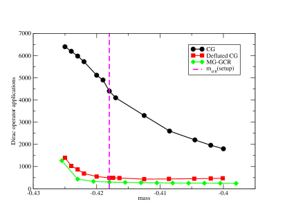
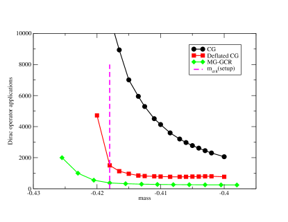
Figure 2: Comparison of CG, deflated CG[5] and MG-GCR total number of Wilson matrix-vector operations until convergence (point sources, $V=16^{3}\times 64$ (left plot), $V=24^{3}\times 64$ (right plot), $\beta=5.5$, $m_{crit}=-0.4175$, $N_{v}=20$ (MG-GCR), $N_{v}=240$ (deflated CG), solver tolerance $=10^{-8}|b|$).

With $N_{\nu}=20$ trial near null vectors this is a very successful multigrid method as illustrated in Fig. 3. The horizontal line is the set up cost of constructing the multigrid operator. Table 1 shows that the iteration count is nearly independent of lattice size and the quark mass, down to the physical pion mass ($m=-.4155$).

We are still at the beginning of additional improvements. For example we have recently combined the multigrid algorithm with red/black preconditioning yielding an additional 30% improvement and we are experimenting with exposing the full Dirac spin structure (not just the chiral structure) on the coarser blocks. It should be noted that our choices were guided to a degree by physical intuition based on chiral symmetry and the ’t Hooft null states associate with isolated instantons but to date there is no precise physical understanding or rigorous mathematical analysis to explain the success of multigrid QCD. Further experimentation and more refined applied mathematical tools are needed to approach an optimal method.

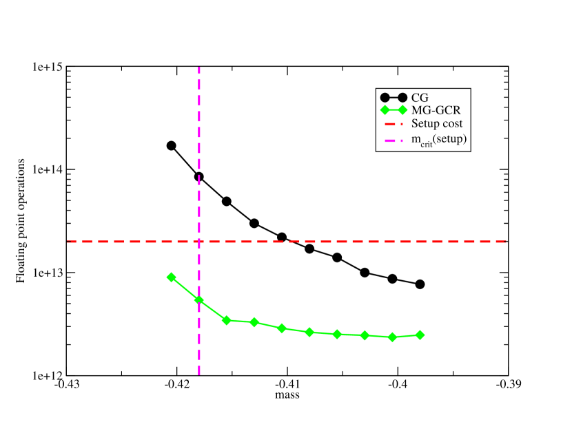
Figure 3: Comparison of adaptive MG algorithm with the conventional red/black preconditioned CG algorithm on $32^{3}\times 96$ lattice.

Mass:	$16^{3}\times 64$	$24^{3}\times 64$	$32^{3}\times 96$
-.3980	40	40	41
-.4005	41	41	42
-.4030	42	42	43
-.4055	42	43	43
-.4080	43	44	45
-.4105	44	46	49
-.4130	45	49	52
-.4155	47	54	57

Table 1: Fine grid iteration count as function of lattice size and quark mass.

4 Future directions

Let us turn to future directions we are pursuing with the caveat that until we have constructed and benchmarked these extensions, the improvements are speculations based on our current experience. First we have begun to design algorithms for both Staggered and Domain Wall fermion discretizations. For Staggered fermions the technical barrier appears modest, since the operator is normal and anti-Hermitian in the chiral limit. However the “species doubling” quadruples the size of the near null space and the Asqtad or HISQ improvements increase the potential complexity of the coarsening. Still with the much larger lattices in production we expect to find a very useful implementation. For the Domain Wall the technical issues are much more subtle but a strategy is emerging. The operator is not only non-Hermitian but the eigenvalues do not have positive real parts as was the case for Wilson and Staggered fermions. Indeed it is essentially a 5-d Wilson operator with the wrong sign mass. However the potential advantage of Domain Wall multigrid is greater. The 5 dimensional Domain Wall matrix operates in a larger vector space and is less well conditioned because of the heavy flavor modes in the 5th dimension, but its near null space is still four dimensional. Thus the truncation to the coarse lattice is more dramatic and in principle there is more to be gained in a multigrid algorithm. Similar remarks hold for the overlap formulation of the Dirac operator but the outer iteration has the advantage of being a normal matrix with positive real mass gap.

A complete suite of multigrid algorithms for Staggered, Wilson and chiral fermion actions holds out the promise of a major reduction in the cost of Dirac inverters for the analysis stage of lattice QCD ensembles. As the physics correlators for lattice QCD have expanded in the USQCD collaborations the relative number of flops devoted to analysis is now exceeding 50%. In addition the multigrid kernel can be used in a variance reduction strategy for stochastic estimators of disconnected quark diagrams [6].We are also beginning to develop inverters compliant with the SciDAC API for general distribution. Firsts we are extending the API to accommodate the multiple lattices and to implement the interpolation and prolongation operators. Also we are optimizing the $N_{\nu}\times N_{\nu}$ complex matrix operations needed for the coarse operators. These algorithms will be freely distributed on the SciDAC software webpages.

In principle MG inverters can be implemented in HMC codes for generating lattice ensembles as well. A critical step in this application is to amortize the set up cost of constructing the coarse operators as the gauge fields evolve in molecular dynamics time. In this regard Lüscher has demonstrated [7] that the subspace update for his “little Dirac” operator (which is essentially equivalent to our first coarse operator $\hat{D}$) can be used for several HMC time steps combined with a chronological procedure for incremental change in the near null space. This strongly suggests that the construction of the multigrid inverter is not a serious overhead. Efficient parallel code is of course another requirement.

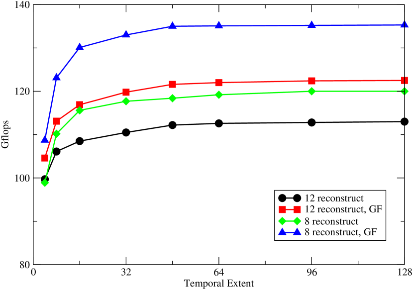
Figure 4: Performance of single precision even-odd preconditioned Wilson-Dirac matrix-vector product on a GTX 280  [8]. GF denotes temporal gauge fixing (lattice volume = $24^{3}\times\mbox{Temporal Extent}$).

Kernel	Kernel	CG	BiCGstab
Prec.	(Gflops)	(Gflops)	(Gflops)
Half 12	202.2	170.6	152.5
SP 8	134.1	110.1	105.1
SP 12	122.1	102.4	98.6
DP 12	35.4	33.5	29.3

Table 2: Performance comparison of the matrix-vector kernels with the associated CG and BiCGstab solvers on the GeForce GTX 280 (lattice volume = $24^{3}\times 48$) [8]. Gauge field stored as 12 or 8 floats.

Finally it is worth closing with a comment on GPU computing. At Boston University we have implemented a highly efficient Wilson Dirac CG and BiCGstab implementations for the Nvidia GPU written in the CUDA extension of C [8]. This gives roughly a 5x advantage in cost performance for Dirac inversions (see Fig. 4). Preliminary analysis indicates that in many ways this architecture is well suited for the multigrid inverter discussed above. The full implementation of this in efficient code has begun and if successful promises a multiplicative advantage in cost per Dirac inverter as the product of hardware and algorithm advances. Even without extensions to the generation of lattices the combined effect of GPU and MG has the potential of dropping the cost of analysis of these lattices by several orders of magnitude relative to current practices.

- [1] For a review of earlier work see: T. Kalkreuter, “Multigrid methods for propagators in lattice gauge theories,” J. Comput. Appl. Math. 63, 57 (1995) [arXiv:hep-lat/9409008].
- [2] R. C. Brower, R. G. Edwards, C. Rebbi and E. Vicari, “Projective multigrid for Wilson fermions,” Nucl. Phys. B 366, 689 (1991).
- [3] M. Brezina, R. Falgout, S. MacLachlan, T. Manteuffel, S. McCormick, and J. Ruge. Adaptive smoothed aggregation (SA). Siam J. Sci. Comput., 25:1896–1920, 2004.
- [4] J. Brannick, R. C. Brower, M. A. Clark, J. C. Osborn and C. Rebbi, “Adaptive Multigrid Algorithm for Lattice QCD,” Phys. Rev. Lett. 100 (2008) 041601 [arXiv:0707.4018 [hep-lat]].
- [5] A. Stathopoulos and K. Orginos, “Computing and deflating eigenvalues while solving multiple right hand side linear systems in Quantum Chromodynamics,” arXiv:0707.0131 [hep-lat].
- [6] R. Babich, R. Brower, M. Clark, G. Fleming, J. Osborn and C. Rebbi, “Strange quark contribution to nucleon form factors,” [arXiv:0710.5536 [hep-lat]].
- [7] M. Luscher, “Deflation acceleration of lattice QCD simulations,” JHEP 0712, 011 (2007) [arXiv:0710.5417 [hep-lat]].
- [8] M. A. Clark, R. Babich, K. Barros, R. C. Brower and C. Rebbi, “Solving Lattice QCD systems of equations using mixed precision solvers on GPUs,” arXiv:0911.3191 [hep-lat].