The Square Root Depth Wave Equations

Abstract

We introduce a set of coupled equations for multilayer water waves that removes the ill-posedness of the multilayer Green-Naghdi (MGN) equations in the presence of shear. The new well-posed equations are Hamiltonian and in the absence of imposed background shear they retain the same travelling wave solutions as MGN. We call the new model the Square Root Depth ($\sqrt{D}$) equations, from the modified form of their kinetic energy of vertical motion. Our numerical results show how the $\sqrt{D}$ equations model the effects of multilayer wave propagation and interaction, with and without shear.

1 Introduction

The propagation and interactions of internal gravity waves on the ocean thermocline may be observed in many areas of strong tidal flow, including the Gibraltar Strait and the Luzon Strait. These waves are strongly nonlinear and may even be seen from the Space Shuttle [10], with their crests moving in great arcs hundreds of kilometres in length and traversing sea basins thousands of kilometres across. The MGN model — the multilayer extension of the well known Green-Naghdi equations [5, 4] — has been used with some success to model the short term behaviour of these waves [8]. Nevertheless, MGN and its rigid-lid version, the Choi-Camassa equation [1996, hereafter CC], have both been shown by Liska & Wendroff [9] to be ill-posed in the presence of background shear. That is, background shear causes the linear growth rate of a perturbation to increase without bound as a function of wave number. Needless to say, this ill-posedness has made numerical modelling of MGN problematic. In particular, ill-posedness prevents convergence of the numerical solution, since the energy cascades to smaller scales and builds up at the highest resolved wave number. Grid refinement only makes the problem worse. Regularization by keeping higher-order expansion terms is possible [1], but such methods tend to destroy the Hamiltonian property of the system and thus may degrade its travelling wave structure. Nevertheless, if one is to consider the wave generation problem, one must consider the effects of both topography and shear.

Thus, the MGN equations must be modified to make them well-posed. We shall require that the new system:

1. is both linearly well-posed and Hamiltonian;

2. preserves the MGN linear dispersion relation for fluid at rest;

3. has the same travelling wave solutions as MGN in the absence of imposed background shear.

The $\sqrt{D}$ equation we introduce here satisfies these requirements. The remainder of the paper is organised as follows. In Section 2 we derive the $\sqrt{D}$ model in the same Euler-Poincaré variational framework as for MGN [11]. In Section 3 we compare the linear dispersion analysis of $\sqrt{D}$ and MGN, and thus show that linear ill-posedness has been removed. In Section 4 we show that the $\sqrt{D}$ and the shear free MGN equations possess the same travelling wave solutions. In Section 5 we present numerical results that compare the wave propagation and interaction properties of the $\sqrt{D}$ and GN solutions for a single layer. Finally, in Section 6 we present numerical results for the $\sqrt{D}$ equations that model the effects of two-layer wave propagation and interaction, both with and without a background shear.

2 The $\sqrt{D}$ Governing Equations

In this section we derive the $\sqrt{D}$ equations by approximating the kinetic energy of vertical motion in Hamilton’s principle for a multilayer ideal fluid. Such a system consists of $N$ homogeneous fluid layers of densities $\rho_{i}$, $i\in[1,\ldots N]$, where $i=1$ is the top layer and $i=N$ is the bottom layer. Thus, for stable stratification, $\rho_{i+1}>\rho_{i}$. The $i$-th layer has a horizontal velocity, $\bm{u}_{i}$ and thickness, $D_{i}$; the interface between the $i$-th and $i-1$-th layer is at depth $h_{i}=-b+\sum_{j=i}^{N}D_{i}$, for a prescribed bathymetry, $b(x,y)$. We assume columnar motion within each layer (horizontal velocity independent of vertical coordinate, $z$). Incompressibility then implies that vertical velocity is linear in $z$. Under this ansatz and after a vertical integration, the Lagrangian for Euler’s fluid equations with a free surface becomes,

$$\ell=\sum_{i=1}^{N}\frac{\rho_{i}}{2}\int\left[D_{i}|\bm{u_{i}}|^{2}+\frac{D_{i}}{3}\left(w_{i}^{2}\Big{|}_{z=\mathchoice{\hbox to0.0pt{$\displaystyle{h_{i+1}}$\hss}}{\hbox to0.0pt{$\textstyle{h_{i+1}}$\hss}}{\hbox to0.0pt{$\scriptstyle{h_{i+1}}$\hss}}{\hbox to0.0pt{$\scriptscriptstyle{h_{i+1}}$\hss}}}\,+\,w_{i}\Big{|}_{z=\mathchoice{\hbox to0.0pt{$\displaystyle{h_{i}}$\hss}}{\hbox to0.0pt{$\textstyle{h_{i}}$\hss}}{\hbox to0.0pt{$\scriptstyle{h_{i}}$\hss}}{\hbox to0.0pt{$\scriptscriptstyle{h_{i}}$\hss}}}\;w_{i}\Big{|}_{z=\mathchoice{\hbox to0.0pt{$\displaystyle{h_{i+1}}$\hss}}{\hbox to0.0pt{$\textstyle{h_{i+1}}$\hss}}{\hbox to0.0pt{$\scriptstyle{h_{i+1}}$\hss}}{\hbox to0.0pt{$\scriptscriptstyle{h_{i+1}}$\hss}}}\;+\,w_{i}^{2}\Big{|}_{z=h_{i}}\right)-g[h_{i}^{2}-h_{i+1}^{2}]\right]\mathrm{d}x\,\mathrm{d}y.$$ (1)

In this Lagrangian, the $w_{i}$ should be viewed as functions of layer velocities, layer thicknesses and their partial derivatives. The fluid momentum equations are obtained from Euler-Poincaré theory [7] as

$$\frac{\partial}{\partial t}\frac{\delta\ell}{\delta\bm{u}_{i}}+\nabla\cdot\left[\bm{u}_{i}\frac{\delta\ell}{\delta\bm{u}_{i}}\right]+\nabla\bm{u}_{i}^{T}\cdot\frac{\delta\ell}{\delta\bm{u}_{i}}=D_{i}\nabla\frac{\delta\ell}{\delta D_{i}}.$$

The system is closed by the layer continuity equations,

$$\frac{\partial D_{i}}{\partial t}+\nabla\cdot D_{i}\bm{u}_{i}=0.$$ (2)

To obtain the MGN equations one sets $w_{i}$ in (1) equal to the vertical component of the fluid velocity, represented in terms of the material time derivative as

$$w_{i} =(h_{i}-z)\nabla\cdot\bm{u}_{i}+\bm{u}_{i}\cdot\nabla h_{i}-\sum_{\mathchoice{\hbox to0.0pt{\hss$\displaystyle{j=i}$\hss}}{\hbox to0.0pt{\hss$\textstyle{j=i}$\hss}}{\hbox to0.0pt{\hss$\scriptstyle{j=i}$\hss}}{\hbox to0.0pt{\hss$\scriptscriptstyle{j=i}$\hss}}}^{N}\nabla\cdot D_{j}\bm{u}_{j}\,.$$ (3)

In each layer, we define a vertical material coordinate, $0\leq s_{i}\leq 1$, by $s_{i}=(h_{i}-z)/D_{i}$. Then, by using $ds_{i}/dt_{i}+w\partial{s_{i}}/\partial z=0$ with $d/dt_{i}=(\partial/\partial t+\bm{u}_{i}\cdot\nabla)$, we note

$$w_{i}=D_{i}\frac{ds_{i}}{dt_{i}}.$$ (4)

To obtain the new $\sqrt{D}$ equations, we replace $w_{i}$ in (1) with a different linear approximation of the vertical motions within each layer, as follows

$$W_{i} =\frac{d_{i}}{D_{i}}\left(\frac{\partial h_{i}}{\partial t}-\frac{(h_{i}-z)}{D_{i}}\frac{\partial D_{i}}{\partial t}\right)=d_{i}\frac{\partial s_{i}}{\partial t}\>.$$ (5)

This approximation introduces a set of $N$ new length scales, $d_{i}$, the far field fluid thicknesses. The final quantity in (5) is a vertical fluid velocity, expressed in the convective representation [6]. The spatial and convective representations of fluid dynamics are the analogues, respectively, of the spatial and body representations of rigid body dynamics on $SO(3)$. This analogy arises because the configuration spaces for fluid dynamics and for rigid bodies are both Lie groups. In both cases, spatial velocities are right-invariant vector fields, while the convective, or body, velocities are the corresponding left-invariant vector fields.

On taking variations, the final equations arising from Hamilton’s principle for the new Lagrangian may be written compactly in terms of a shallow water equation, plus additional nonlinear dispersive terms that represent a non-hydrostatic pressure gradient,

$$\frac{\partial\bm{u}_{i}}{\partial t}+\bm{u}_{i}\cdot\nabla\bm{u}_{i}=-g\nabla\underbrace{\left[h_{i}+\sum_{j=1}^{i-1}\frac{\rho_{j}}{\rho_{i}}D_{j}\right]}_{\hbox{hydrostatic\ pressure}}-\ \nabla\underbrace{\left[\frac{d_{i}F_{i}}{6}+\sum_{j=1}^{i-1}\frac{\rho_{j}d_{j}G_{j}}{2\rho_{i}}+\frac{d_{i}^{2}E_{i}}{6D_{i}^{2}}\right]}_{\hbox{non-hydrostatic\ pressure}},$$ (6)

$$F_{i}=\left(\frac{\partial}{\partial t}\frac{d_{i}}{D_{i}}\frac{\partial}{\partial t}\right)\left[2h_{i}+h_{i+1}\right],\quad G_{i}=\left(\frac{\partial}{\partial t}\frac{d_{i}}{D_{i}}\frac{\partial}{\partial t}\right)\left[h_{i}+h_{i+1}\right],$$

$$E_{i}=\left(\frac{\partial h_{i}}{\partial t}\right)^{2}+\frac{\partial h_{i}}{\partial t}\frac{\partial h_{i+1}}{\partial t}+\left(\frac{\partial h_{i+1}}{\partial t}\right)^{2}.$$

In comparison, the MGN equations have a similar form, but the non-hydrostatic forces no longer correspond to the gradient of a pressure. Instead, the MGN equations take the form

$$\frac{\partial\bm{u}_{i}}{\partial t}+\bm{u}_{i}\cdot\nabla\bm{u}_{i}=-g\nabla\left[h_{i}+\sum_{j=1}^{i-1}\frac{\rho_{j}}{\rho_{i}}D_{j}\right]-\frac{1}{D_{i}}\nabla\frac{D_{i}^{2}\widetilde{F}_{i}}{6}-\nabla\sum_{j=1}^{i-1}\frac{\rho_{j}D_{j}\widetilde{G}_{j}}{2\rho_{i}}-\frac{1}{2}\widetilde{G}_{i}\nabla h_{i+1},$$ (7)

$$\widetilde{F_{i}}=\left(\frac{\partial}{\partial t}+\bm{u}_{i}\cdot\nabla\right)^{2}\left[2h_{i}+h_{i+1}\right],\quad\widetilde{G_{i}}=\left(\frac{\partial}{\partial t}+\bm{u}_{i}\cdot\nabla\right)^{2}\left[h_{i}+h_{i+1}\right].$$

Having arisen from Hamilton’s principle, the $\sqrt{D}$ and MGN equations may both be written in Hamiltonian form. In addition, since their Lagrangians are both invariant under particle relabelling, the two sets of equations each possesses the corresponding materially-conserved quantities,

$$\frac{\partial q_{i}}{\partial t}+\bm{u}_{i}\cdot\nabla{q}_{i}=0,\quad\hbox{where}\quad q_{i}:=\frac{1}{D_{i}}\bm{\hat{z}}\cdot\nabla\times\left(\frac{1}{D_{i}}\frac{\delta\ell}{\delta\bm{u}_{i}}\right).$$

The quantity $q_{i}$ is the potential vorticity in the $i$-th layer. For the $\sqrt{D}$ equations,

$$q_{i}=\bm{\hat{z}}\cdot\left(\nabla\times\bm{u}_{i}\right)/D_{i},$$

just as for the unmodified shallow water equations. Hence, equation (6) admits potential flow solutions for which $\nabla\times\bm{u}_{i}=0$. In contrast, the MGN potential vorticity contains higher derivatives of $\bm{u}_{i}$.

When restricted to a single layer, the Lagrangian for the $\sqrt{D}$ equations (6) is

$$\ell=\frac{\rho}{2}\int D|\bm{u}|^{2}+\frac{4d^{2}}{3}\left(\frac{\partial}{\partial t}\sqrt{D}\right)^{2}-g\left[\left(D-b\right)^{2}-b^{2}\right]\mathrm{d}x\,\mathrm{d}y,$$

and the single-layer $\sqrt{D}$ motion equation becomes

$$\frac{\partial\bm{u}}{\partial t}+\bm{u}\cdot\nabla\bm{u}=-g\nabla\left(D-b\right)-\frac{d^{2}}{6}\nabla\left(\frac{1}{\sqrt{D}}\frac{\partial^{2}\sqrt{D}}{\partial t^{2}}\right).$$

The single-layer Lagrangian contains a term that coincides with the Fisher-Rao metric in probability theory. (See Brody & Hughston [2] for an excellent review of the subject.) This feature suggested the name “$\sqrt{D}$ equations” for the new system.

3 Linear Dispersion Analysis

This section shows that the $\sqrt{D}$ equations in (6) possess the same linear dispersion relation at rest as MGN, but that unlike MGN they remain linearly well-posed when background shear is present. As discussed in Liska & Wendroff [9], linear well-posedness requires that the phase speed remain bounded as $k\to\infty$ for all background shear profiles. In what follows we specialise to the case $N=2$, and impose a rigid lid constraint, $h_{1}=0$, through an additional barotropic pressure term, although the analysis generalizes to an arbitrary number of layers and to the free surface case. Linearizing equations (6) and (2) for far field depths, $d_{1}$, $d_{2}$ and background velocities, $U_{1}$, $U_{2}$ produces the following dispersion relation

$$\rho_{1}d_{2}\left(U_{1}-\lambda\right)^{2}+\rho_{2}d_{1}\left(U_{2}-\lambda\right)^{2}+\left({\lambda^{2}k^{2}d_{1}d_{2}}/{3}\right)\left(\rho_{1}d_{1}+\rho_{2}d_{2}\right)-(\rho_{2}-\rho_{1})gd_{1}d_{2}=0.$$

Here the phase speed is $\lambda=\omega/k$ for frequency $\omega$ and wave number $k$. Meanwhile under the same assumptions the equivalent CC equations linearize to

$$\rho_{1}d_{2}\left(U_{1}-\lambda\right)^{2}\left(1+{d_{1}k^{2}}/{3}\right)+\rho_{2}d_{1}\left(U_{2}-\lambda\right)^{2}\left(1+{d_{2}k^{2}}/{3}\right)-(\rho_{2}-\rho_{1})gd_{1}d_{2}=0.$$

When the background state is at rest, $U_{1}=U_{2}=0$, both sets of equations exhibit the same dispersion relation,

$$\lambda=\frac{\pm\sqrt{\left(\rho_{2}-\rho_{1}\right)gd_{1}d_{2}}}{\sqrt{\rho_{1}d_{2}+\rho_{2}d_{1}+\left(\rho_{1}d_{1}+\rho_{2}d_{2}\right)d_{1}d_{2}k^{2}}},$$

in which the phase speed of the high wave number modes converges towards zero. This is not surprising, since when linearized at rest the two measures of vertical motion coincide in (3) and (5), with $w_{i}=W_{i}$.

In the presence of background shear, $U_{1}\neq U_{2}$, the solution for the phase speed $\lambda$ of the rigid lid $\sqrt{D}$ equations is

$$\lambda =\frac{-B_{0}\pm\sqrt{B_{0}^{2}-4\left(A_{0}+A_{2}k^{2}\right)\left(C_{0}-(\rho_{2}-\rho_{1})gd_{1}d_{2}\right)}}{2\left(A_{0}+A_{2}k^{2}\right)},$$

$$\sim\pm\frac{\sqrt{\left(C_{0}-(\rho_{2}-\rho_{1})gd_{1}d_{2}\right)}}{\sqrt{A_{2}}|k|}\qquad\textrm{for }k\gg 1$$

and for the CC equations is

$$\lambda =\frac{-\left(B_{0}+B_{2}k^{2}\right)\pm\sqrt{\left(B_{0}+B_{2}k^{2}\right)^{2}-4\left(A_{0}+A_{2}k^{2}\right)\left(C_{0}+C_{2}k^{2}-(\rho_{2}-\rho_{1})gd_{1}d_{2}\right)}}{2\left(A_{0}+A_{2}k^{2}\right)},$$

$$\sim\frac{-B_{2}\pm\sqrt{B_{2}^{2}-4A_{2}C_{2}}}{2A_{2}}\qquad\textrm{for }k\gg 1.$$

Here the coefficients $A_{0}$, $B_{0}$, $C_{0}$, etc. are functions of the mean depth ratio, $d_{1}/d_{2}$ and of the shear $(U_{2}-U_{1})$. Liska & Wendroff [9] showed that the discriminant $B_{2}^{2}-A_{2}C_{2}$ is strictly negative in the CC case, thereby ensuring the existence of a root with growth rate, $\Im(\lambda k)$, which is positive and scales linearly with $k$. Thus, the CC equations are linearly ill-posed. In contrast, the magnitude of growth rates in the $\sqrt{D}$ case are bounded from above, independently of wave number $k$. Thus, the $\sqrt{D}$ equations are linearly well-posed. Indeed, provided a Richardson-number condition is satisfied, that

$$Ri:=\left(\rho_{2}-\rho_{1}\right)gd_{1}d_{2}\left(d_{1}+d_{2}\right)^{2}/\Big{[}\left(\rho_{1}d_{2}^{3}+\rho_{2}d_{1}^{3}\right)|U_{2}-U_{1}|^{2}\Big{]}\geq 1,$$ (8)

then the linearized system remains stable to perturbations at any wave number.

4 Travelling Wave Solutions

At this point, we have shown that the $\sqrt{D}$ equations satisfy requirements (a) and (b) in the Introduction. We will now show that the $\sqrt{D}$ and MGN equations also satisfy requirement (c); that is, they share the same travelling wave solutions for any number of layers, in the absence of imposed background shear. We take a travelling wave ansatz for a choice of wave speed, $c$,

$$D_{i}(x,t)=:D_{i}(X),\quad u_{i}(x,t)=:u_{i}(X),\quad\hbox{with}\quad X:=x-ct\,.$$

Integrating the continuity equation (2) in a frame moving at the mean barotropic velocity implies for both the MGN and $\sqrt{D}$ systems that

$$u_{i}=c\left(1-{d_{i}}/{D_{i}}\right).$$ (9)

For such solutions we see from equations (3) and (5) that $w_{i}$ and $W_{i}$ coincide,

$$w_{i}=(h_{i}-z)\frac{\partial u_{i}}{\partial X}+(u_{i}-c)\frac{\partial h_{i}}{\partial X}=-\frac{cd_{i}}{D_{i}}\left[\frac{(z-h_{i})}{D_{i}}\frac{\partial D_{i}}{\partial X}+\frac{\partial h_{i}}{\partial X}\right]=W_{i}.$$ (10)

To obtain travelling wave solutions, one varies the Lagrangian subject to the relation (9). Using relation (10) between the vertical velocities implies that the travelling wave Lagrangians for the $\sqrt{D}$ and MGN equations coincide. Consequently, the travelling wave solutions of the two equation sets must also coincide. This finishes the derivation of the new equation set and the verification of the three requirements set out in the Introduction. In the presence of background shear, however, $(w_{i}-W_{i})\neq 0$, and the coincidence of the travelling waves of the two models no longer holds.

5 Numerical experiments (Single layer)

We now present some results of numerical computation with the $\sqrt{D}$ equations for a single layer. The equations are discretized using standard finite volume techniques, without any filtering. In this section we compare results for the one-layer $\sqrt{D}$ and GN equations. These results show that the two systems have the same qualitative behaviour.

5.1 Single layer lock release

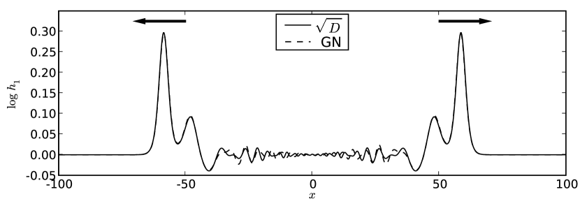
Figure 1: Single-layer $\sqrt{D}$ and GN thickness profiles arising from lock-release runs. The arrows indicate directions of crest propagation. The leading wave profiles are essentially identical for both the $\sqrt{D}$ and GN equations. The smaller crests are also very similar. (Differences are emphasised by using a logarithmic scale.)

We first consider a lock release experiment with periodic boundary conditions and physical parameters and initial conditions given by

$$d=1,\quad g=1,$$

$$D(x,0)=1+0.5\left[\tanh\left(x-4\right)-\tanh\left(x+4\right)\right],\quad u(x,0)=0,\quad x\in[-100,100].$$

We integrated this state forwards in time for both the GN and $\sqrt{D}$ systems. Figure 1 shows a snapshot of a train of travelling waves emerging from the lock release in each equation set. In both cases, the first wave is the largest and the wave profiles of the two systems track each other closely. This may have been expected, because the two systems share the same travelling wave solutions and possess identical linear dispersion relations for a quiescent background.

5.2 Single layer interaction of solitary waves

We now consider the interaction between pairs of solitary travelling wave solutions in the two systems. The $\sqrt{D}$ and GN systems have the same travelling wave solutions, but their PDEs differ; so one may expect to see differences in their wave-interaction properties. For both systems the travelling wave takes a $\textrm{sech}^{2}$ form,

$$D=d\left[1+\left(\frac{c^{2}}{gd}-1\right)\textrm{sech}^{2}\left(\frac{\sqrt{3\left(c^{2}-gd\right)}\left(x-ct\right)}{2cd}\right)\right],$$

and the velocity profile is given by equation (9). Figure 2 shows a snapshot of the results for the case of two equal amplitude, oppositely directed travelling waves after suffering a symmetric head-on collision. Both the $\sqrt{D}$ and GN descriptions show a near-elastic collision followed by small-amplitude radiation. The travelling wave behaviour is essentially identical. The main difference lies in the details of the slower linear waves that are radiated and left behind during the nonlinear wave interactions. Similar results were obtained in the case of asymmetric collisions.

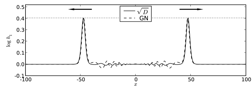
Figure 2: Single-layer $\sqrt{D}$ and GN results are shown for symmetric head-on collision experiments. Layer thickness profiles are shown after the collision. The fully nonlinear collision is near elastic for both $\sqrt{D}$ and GN, with near conservation of the initial amplitude, shown by the dotted line. The travelling wave behaviour is essentially the same, except for a very small phase shift, while the slow, small-amplitude radiation waves show a few minor differences.

6 Numerical Experiments (Two Layers, Rigid Lid)

We now consider numerical solutions of the two-layer rigid lid $\sqrt{D}$ equations in one spatial dimension. Unlike the result of Jo & Choi [8] for the CC equations, there is no value of resolution at which the code for numerically integrating the $\sqrt{D}$ equations becomes unstable. This might have been hoped, because the $\sqrt{D}$ equations are linearly well-posed.

6.1 Two layer rigid lid lock release experiments

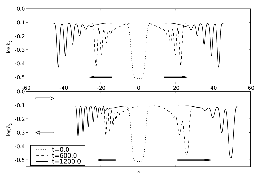
Figure 3: Two-layer rigid lid lock release experiments are compared, with and without background shear of Richardson number $Ri=5.02$. The fluid interface is plotted at times $t=0$, 600, 1200. Here $g=1$, $\rho_{1}/\rho_{2}=0.995$, $d_{1}/h_{1}=0.1$. The fluid was initialised with a symmetric tanh profile in thickness. Filled arrows denote the directions of travel of the waves, while unfilled arrows indicate the background shear. The run without shear (upper figure) generated a left-right symmetric distribution of wave crests. In contrast, the run with background shear (lower figure) generated an asymmetric distribution of wave peaks. The lower figure shows lock release for an upper layer moving with initially constant rightward velocity. Consequently, there was a net transfer of momentum toward the right, which significantly affected the distribution of wave crests.

We next present the result of the equivalent lock-release experiment to that of Section 5.1 for the two-layer rigid lid equations in lock release configuration. For this, we choose $d_{1}=0.1$, $d_{2}=0.9$, $g=1$, and

$$D_{1}(x,0)=d_{1}+0.3\left[\tanh\left(x-4\right)-\tanh\left(x+4\right)\right],\;D_{2}=d_{1}+d_{2}-D_{1},\;x\in[-100,100].$$

The initial configuration is taken as a depression of the fluid interface, because CC or $\sqrt{D}$ travelling waves extend from the thinner layer into the thicker one. Since our motivating interest was in modelling waves on the ocean thermocline, we will concentrate here on the situation in which the top layer is thinner than the bottom layer. We show results for the following velocity profiles:

1. No shear: $u_{1}(x,0)=0$, $u_{2}(x,0)=0$, and $x\in[-100,100]$.

2. Background shear flow: $u_{1}(x,0)=0.01$, $u_{2}=-{D_{1}u_{1}}/{D_{2}}$,amd $x\in[-100,100].$

From (8) the Richardson number for the case with shear is $Ri=5.02$, and the flow is still linearly stable for all wave numbers.

The result of the integration is shown in Figure 3. Unlike the single-layer case, the linear long wave speed in the two-layer case is close to the wave speed of the resulting travelling waves. In Figure 4 we compare the leading short wave disturbances of one lobe in the shear-free lock-release experiment to the calculated solitary travelling wave solutions in the same parameter regime, as defined by the maximum amplitude of the disturbance. For the three largest waves the differences are indistinguishable, while the smaller waves, which are still interacting with the long wave signal are wider than the equivalent true travelling wave. A similar result holds for the asymmetric crests generated in the presence of shear and for the respective velocity profiles. The leading order solution is thus well approximated as a train of independent solitary travelling waves propagating in order of amplitude.

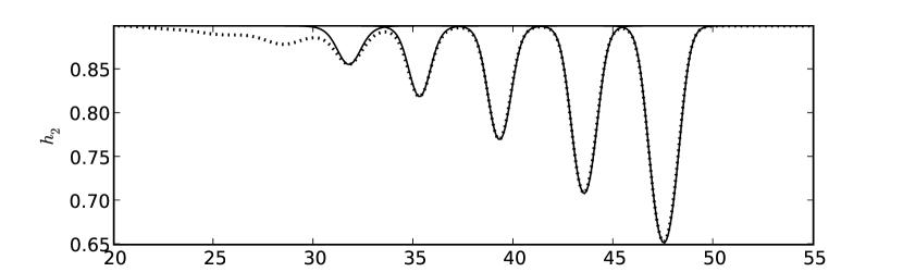
Figure 4: Close up of two-layer wave lock-release experiment in Figure 3. The corresponding travelling wave profile (solid line, as defined by the maximum wave amplitude) is plotted over the numerical lock-release solution at t=1300 (dashed line). In the three leading waves, the differences from the corresponding solitary wave profiles are indiscernible.

6.2 Interaction of two layer solitary waves with rigid lid

Finally we consider wave interaction experiments in the two-layer case. Here we initialize with two numerical solutions of the travelling wave problem with oppositely directed velocities. Results for these two experiments are similar to those in the single layer case and also similar to those in Jo & Choi [8] in the case without shear. Figure 5 shows our numerical solution following the wave collision in the case of equal magnitude wave speed with and without a background shear. We again see nearly elastic collisions, after which the waves approximately regain both their shape and amplitude. In the case with shear, the wave profiles are no longer symmetric. Defining upstream and downstream direction in terms of the background flow in the thicker layer, we see that the upstream gains amplitude and narrows compared with the shear-free wave profile at the same wave speed, while the wave travelling upstream loses amplitude and widens. Nevertheless, the waves are seen to nearly conserve amplitude, and hence momentum through the collision.

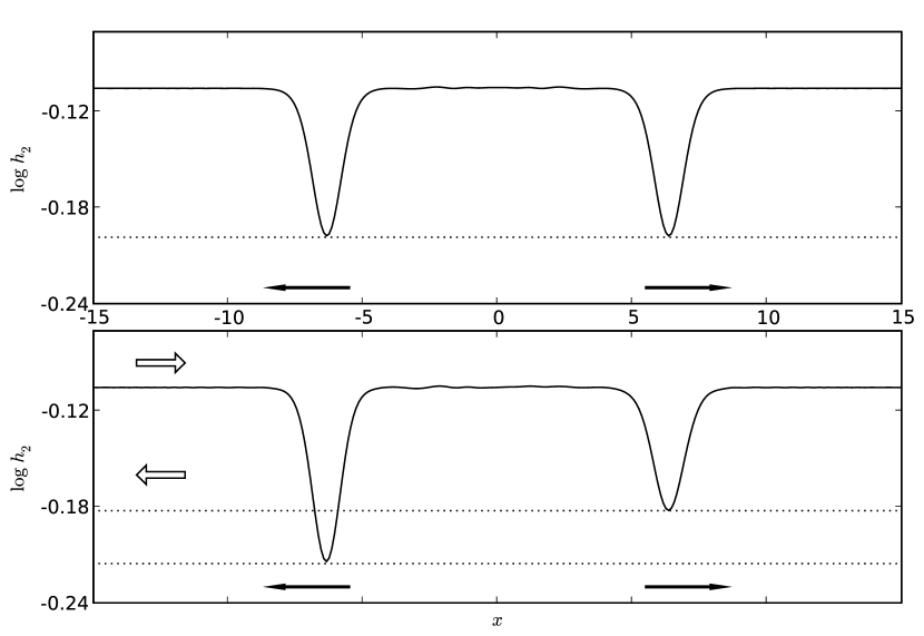
Figure 5: The figure shows two-layer head-on collision experiments with a rigid lid. In the top figure there is no background shear, while in the bottom figure the Richardson number is $Ri=502$. The interface depth is shown after the symmetric head-on collision of two travelling waves of the same phase speed. Physical parameters are, $g=1$, $\rho_{1}/\rho_{2}=0.995$, $d_{1}/h_{1}=0.1$. In both figures the phase velocity is $c/\sqrt{gh_{1}}=\pm 0.027$ and the initial amplitudes are indicated by dotted lines. Filled arrows denote the directions in which the solitary waves are travelling, while unfilled arrows indicate the background shear. In both cases, the collision was found to be nearly elastic, and the final conditions were essentially mirror reflections of the initial conditions, with only slight changes in the amplitudes.

7 Summary

We have introduced a system of Hamiltonian multilayer water wave equations that is linearly well-posed in the presence of background shear but possesses the same travelling wave solutions as the MGN equations, whose ill-posedness had previously caused difficulties in their numerical integration. The new system also has been found numerically to generate fast-moving trains of large-amplitude coherent waves that exhibit ballistic, nearly-elastic, nonlinear scattering behaviour amidst a background of slow, small-amplitude, weakly interacting or linear wave radiation. Future work will explore wave-wave and wave-topography interactions in the presence of vertical shear between the layers, as well as two-dimensional multilayer wave interactions and wave generation by flow over topography by using the new well-posed $\sqrt{D}$ equation set.

We are grateful to W. Choi, F. Dias and R. Grimshaw for fruitful discussions on this topic. J. R. Percival was supported by the ONR grant N00014-05-1-0703.

References

- Barros & Choi [2009] Barros, R. & Choi, W. 2009 Inhibiting shear instability induced by large amplitude internal solitary waves in two-layer flows with a free surface. Studies in Applied Mathematics 122 (3), 325–346.
- Brody & Hughston [1998] Brody, D. C. & Hughston, L. P. 1998 Statistical geometry in quantum mechanics. Proc. Roy. Soc. A 454, 2445–2475.
- Choi & Camassa [1996] Choi, W. & Camassa, R. 1996 Weakly nonlinear internal waves in a two-fluid system. Journal of Fluid Mechanics 313, 83–103.
- Choi & Camassa [1999] Choi, W. & Camassa, R. 1999 Fully nonlinear internal waves in a two-fluid system. Journal of Fluid Mechanics 396, 1–36.
- Green & Naghdi [1976] Green, A. E. & Naghdi, P. M. 1976 A derivation for wave propagation in water of variable depth. Journal of Fluid Mechanics 78, 237–246.
- Holm et al. [1986] Holm, D. D., Marsden, J. E. & Ratiu, T. S. 1986 The Hamiltonian structure of continuum mechanics in material, inverse material, spatial and convective representations. In Hamiltonian Structure and Lyapunov Stability for Ideal Continuum Dynamics. University of Montreal Press,.
- Holm et al. [1998] Holm, D. D., Marsden, J. E. & Ratiu, T. S. 1998 The Euler-Poincaré equations and semi-direct products with applications to continuum therories. Advances in Mathematics .
- Jo & Choi [2002] Jo, T.-C. & Choi, W. 2002 Dynamics of strongly nonlinear internal solitary waves in shallow water. Studies in Applied Mathematics .
- Liska & Wendroff [1997] Liska, R. & Wendroff, B. 1997 Analysis and computation wth stratified fluid models. Journal of Computational Physics 137 (1).
- Liu et al. [1998] Liu, A. K., Chang, Y. S., Hsu, M. K. & Liang, N. K. 1998 Evolution of nonlinear internal waves in the East and South China Seas. Journal of Geophysical Research .
- Percival et al. [2008] Percival, J. R., Holm, D. D. & Cotter, C. J. 2008 A Euler-Poincaré framework for the Green-Naghdi equations. Journal of Physics A: Mathematical and Theoretical 41 (34).