The nuclear energy density functionals with modified radial dependence of the isoscalar effective mass

Abstract

Calculations for infinite nuclear matter with realistic nucleon-nucleon interactions suggest that the isoscalar effective mass (IEM) of a nucleon at the saturation density equals $m^{*}/m\sim 0.8\pm 0.1$, at variance with empirical data on the nuclear level density in finite nuclei which are consistent with $m^{*}/m\approx 1$. This contradicting results might be reconciled by enriching the radial dependence of IEM. In this work four new terms are introduced into the Skyrme-force inspired local energy-density functional: $\tau(\nabla\rho)^{2}$, $\tau\frac{d\rho}{dr}$, $\tau^{2}$ and $\tau\Delta\rho$. The aim is to investigate how they influence the radial dependence of IEM and, in turn, the single-particle spectra.

1 Introduction

The nuclear energy-density functional (EDF) is considered nowadays as one of the most promising theoretical tools to describe static properties of the atomic nuclei. Tremendous effort is undertaken recently to develop high-precision spectroscopic quality functionals. A standard way to construct the nuclear EDF is to start with either the finite-range Gogny [1] or the zero-range Skyrme [2] effective interaction and average it with the density matrix within the Hartree-Fock (HF) method. Such functionals may be further enriched by adding new terms. For instance, Carlsson et al. [3] considered a systematic generalization of the Skyrme functional by introducing terms up to sixth order in derivatives of the density matrix.

Calculations for infinite nuclear matter suggest that the isoscalar effective mass (IEM) at the saturation density should be of order of $m^{*}/m\sim 0.8\pm 0.1$ [4, 5, 6, 7, 8]. On the other hand, description of the single-particle (s.p.) level density in finite nuclei requires the IEM close to unity. This contradicting conditions might be fulfilled together by assuming the IEM smaller than one inside the nucleus and peaked at the surface. Such a concept was first explored by Ma and Wambach [9] in a non-self-consistent model and by Farine et al. [10] within a self-consistent framework. Since it is impossible to obtain a surface-peaked IEM within the standard form of Skyrme functional, in the present paper we examine four simple additional terms that can modify the radial dependence of IEM.

The new terms are introduced in Sec. 2. Sec. 3 reports on the resulting radial dependence of the IEM. In Sec. 4, influence of the new terms on the s.p. spectra is presented. The paper is concluded in Sect. 5. In this exploratory work, we limit our calculations to three spherically symmetric isoscalar nuclei, ⁴⁰Ca, ⁵⁶Ni, and ¹⁰⁰Sn.

2 Extensions to the Skyrme energy-density functional

The Skyrme energy density, ${\mathcal{H}}({\mathbf{r}})$, consists of the kinetic and interaction parts,

$${\mathcal{H}}({\mathbf{r}})=\frac{\hbar^{2}}{2m}\tau_{0}+\displaystyle\sum_{t=0,1}{\mathcal{H}}_{t}({\mathbf{r}}),$$ (1)

where

$$\mathcal{H}_{t}=C^{\rho}_{t}[\rho_{0}]\rho^{2}_{t}+C^{\Delta\rho}_{t}\rho_{t}\Delta\rho_{t}+C^{\tau}_{t}\rho_{t}\tau_{t}+C^{J}_{t}{\mathbb{J}}^{2}_{t}+C^{\nabla J}_{t}\rho_{t}{\mathbf{\nabla}}\cdot{\mathbf{J}}_{t}.$$ (2)

Index $t=0,1$ denotes the isospin, and $C_{t}$ are the coupling constants, of which one, $C^{\rho}_{t}[\rho_{0}]=C^{\rho\prime}_{t}+C^{\rho\prime\prime}_{t}{\rho_{0}}^{\alpha}$, depends on the isoscalar density. The potential energy terms are bilinear forms of the time-even densities, $\rho$, $\tau$, ${\mathbb{J}}$, and their derivatives. The density ${\mathbf{J}}_{t}$ denotes the vector part of the spin-current tensor, ${\mathbf{J}}_{t,\lambda}=\sum_{\mu\nu}\epsilon_{\lambda\mu\nu}{\mathbb{J}}_{t,\mu\nu}$. Readers interested in details are referred, e.g., to Ref. [11].

The central field, $\mathcal{U}({\mathbf{r}})$, is defined as a variation of the energy density with respect to the particle density,

$$\mathcal{U}_{t}({\mathbf{r}})=\frac{\delta[\mathcal{H}({\mathbf{r}})]}{\delta\rho_{t}({\mathbf{r}})}=2C^{\rho}_{t}[\rho_{0}]\rho_{t}+2C^{\Delta\rho}_{t}\Delta\rho_{t}+C^{\tau}_{t}\tau_{t}+C^{\nabla J}_{t}{\mathbf{\nabla}}\cdot{\mathbf{J}}_{t}+\delta_{t0}\,\sum_{t^{\prime}=0,1}\frac{\partial C^{\rho}_{t^{\prime}}}{\partial\rho_{0}}\rho_{t^{\prime}}^{2}.$$ (3)

The effective mass is proportional to the inverse of the mass field, which is a variation of the energy density with respect to the kinetic density,

$$\frac{\hbar^{2}}{2m_{t}^{*}({\mathbf{r}})}=\mathcal{M}_{t}({\mathbf{r}})=\frac{\delta[\mathcal{H}({\mathbf{r}})]}{\delta\tau_{t}({\mathbf{r}})}=\frac{\hbar^{2}}{2m}\delta_{t0}+C^{\tau}_{t}\rho_{t}({\mathbf{r}}).$$ (4)

The IEM is defined as $m_{0}^{*}/m$. It is easily seen from Eq. (4) that in the standard Skyrme functional, the IEM is a monotonic function of the isoscalar particle density, $\rho_{0}$, and therefore cannot be peaked at the surface. The term proportional to $\rho_{0}$ in Eq. (4) can only decrease or increase the IEM in the interior of the nucleus.

Thus, in order to enrich the radial dependence of the IEM, one has to add to the functional new terms depending on the isoscalar kinetic density, $\tau_{0}$. We consider here four such terms,

$${\mathcal{H}}_{0}^{(A)}({\mathbf{r}}) = C_{0}^{\tau(\mathbf{\nabla}\rho)^{2}}\tau_{0}({\mathbf{r}})\left(\mathbf{\nabla}\rho_{0}({\mathbf{r}})\right)^{2},$$ (5)

$${\mathcal{H}}_{0}^{(B)}({\mathbf{r}}) = C_{0}^{\tau\frac{d\rho}{dr}}\tau_{0}({\mathbf{r}})\frac{d\rho_{0}({\mathbf{r}})}{dr},$$ (6)

$${\mathcal{H}}_{0}^{(C)}({\mathbf{r}}) = C_{0}^{\tau^{2}}(\tau_{0}({\mathbf{r}}))^{2},$$ (7)

$${\mathcal{H}}_{0}^{(D)}({\mathbf{r}}) = C_{0}^{\tau\Delta\rho}\tau_{0}({\mathbf{r}})\Delta\rho_{0}({\mathbf{r}}).$$ (8)

These terms will be treated independently and dubbed as variants A, B, C, and D of our model, respectively. Their contributions to the mass field read, respectively,

$${\mathcal{M}}_{0}^{(A)}({\mathbf{r}}) = C_{0}^{\tau(\mathbf{\nabla}\rho)^{2}}\left(\mathbf{\nabla}\rho_{0}({\mathbf{r}})\right)^{2},$$ (9)

$${\mathcal{M}}_{0}^{(B)}({\mathbf{r}}) = C_{0}^{\tau\frac{d\rho}{dr}}\frac{d\rho_{0}({\mathbf{r}})}{dr},$$ (10)

$${\mathcal{M}}_{0}^{(C)}({\mathbf{r}}) = 2C_{0}^{\tau^{2}}\tau_{0}({\mathbf{r}}),$$ (11)

$${\mathcal{M}}_{0}^{(D)}({\mathbf{r}}) = C_{0}^{\tau\Delta\rho}\Delta\rho_{0}({\mathbf{r}}).$$ (12)

All of these terms but ${\mathcal{H}}_{0}^{(C)}$ contribute to the central field as well,

$${\mathcal{U}}_{0}^{(A)}({\mathbf{r}}) = -2C_{0}^{\tau(\mathbf{\nabla}\rho)^{2}}\left(\mathbf{\nabla}\tau_{0}\cdot\mathbf{\nabla}\rho_{0}+\tau_{0}\Delta\rho_{0}\right),$$ (13)

$${\mathcal{U}}_{0}^{(B)}({\mathbf{r}}) = C_{0}^{\frac{d\rho}{dr}}\frac{d\tau_{0}}{dr},$$ (14)

$${\mathcal{U}}_{0}^{(D)}({\mathbf{r}}) = C_{0}^{\tau\Delta\rho}\Delta\tau_{0}({\mathbf{r}}).$$ (15)

The terms A, C, and D are scalars. Hence, their form is natural for all shapes of the nucleus. The term B is valid only in case of spherical symmetry. It is inspired by the Ma and Wambach parameterization of IEM.

The terms A and B depend on the first derivative of the particle density. This derivative is peaked at the surface, so these terms are expected to yield the desired profile of the IEM. Since the gradient square is positive and the radial derivative itself is negative, an upward-pointing peak will require negative and positive values of the coupling constants in cases A and B, respectively.

The term D depends on the second derivative. Hence, it should produce two peaks of opposite signs at the borders of the surface, where the curvature of the density profile is largest.

3 Radial profiles of the isoscalar effective mass

Correct description of the s.p.-level density near the Fermi surface requires the mean value of the IEM to be close to unity. In order to fulfill this condition we impose the following constraint on the radial IEM profile,

$$\int d^{3}{\mathbf{r}}\,\frac{\rho_{0}({\mathbf{r}})}{A}\,\frac{m^{*}({\mathbf{r}})}{m}=1,$$ (16)

where $A$ is the mass number of the considered nucleus.

We examine each of the four new terms, A-D, separately, that is, by switching the remaining three off. In each case, we vary the concerned new coupling constant by hand, and for each value thereof, we readjust the coupling constant $C^{\tau}_{0}$ to fulfill the condition (16). This means that the excess of the IEM produced by the peak is compensated by decreasing the IEM inside the nucleus.

The remaining coupling constants of the functional (2) are kept intact at values of the SkXc Skyrme parameterization [12]. This specific parameterization was chosen because of the condition (16). Indeed, in order to fulfill Eq. (16) it is reasonable to choose a parameterization with the IEM close to unity, which is a case for the SkXc. In addition, this force was fitted with particular attention payed to the s.p. spectra.

It turned out that the possible values of the new coupling constants are limited. Extending the new coupling constants beyond certain limits leads to strong oscillations of the density what causes that the total energy diverges. The radial profiles of the IEM obtained in ⁴⁰Ca for the limiting (both negative and positive) values of the new coupling constants are shown in Fig. 1. The limits corresponding to downward-pointing peaks in the IEM are, most likely, of limited physical interest.

It is clearly seen that in the variants A and B of our model the desired surface-peaked IEM profile is obtained. In the variant C a well pronounced peak appears as well, but it is shifted toward the center of the nucleus. The variant D yields only small fluctuations of the IEM value, and it does not seem to be of much relevance.

Figure 1: Radial dependence of the IEM, $m_{0}^{*}(r)/m$, in ⁴⁰Ca for the four variants of the calculations. The solid and dashed lines show the IEM profiles for the limiting achievable values of the corresponding coupling constants. See text for details.

4 Influence of the new terms on single-particle energies

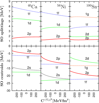
(a)

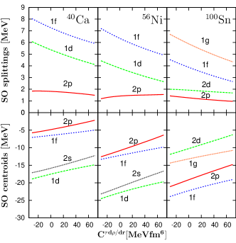
(b)

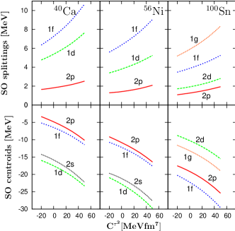
(c)

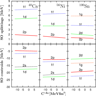
(d)

Figure 2: Spin-orbit splittings (upper panels) and centroids (lower panels) as a function of $C^{\tau\frac{d\rho}{dr}}$ (a) and $C^{\tau\frac{d\rho}{dr}}$ (b), $C^{\tau^{2}}$ (c) and $C^{\tau\Delta\rho}$ (d) in ⁴⁰Ca (left), ⁵⁶Ni (middle) and ¹⁰⁰Sn (right) nuclei.

In our study, we are mostly interested in the influence of the new terms on the s.p. spectra, in particular on the spin-orbit (SO) coupling. For each pair of the SO partners, with the same $n$, $l$, and $j=l\pm\frac{1}{2}$, we define the SO splitting as the difference of their energies, and the SO centroid as the arithmetic average thereof. Figure 2 shows, separately for each variant of our model, the SO splittings and centroids as a function of new coupling constant for the entire accessible range of each coupling constant.

The new terms influence both the SO splittings and centroids quite strongly in all variants of our model except the variant D. In the latter case, the modifications of the IEM’s radial profile are apparently too weak to produce any clear trend. In our calculations, the term C affects the s.p. levels most strongly. However, it also shifts the binding energies of the considered nuclei by more than 50% when going from $C^{\tau^{2}}_{0}=0$ to the limiting values. It is, therefore, clear that in order to remain within a physically acceptable area, it would be necessary to refit all the coupling constants of the functional at least to masses and radii of the three considered nuclei. This is, however, beyond the scope of the present work. Such a problem is of slightly lesser importance for the terms A and B, since their inclusion does not change the masses by more than 10%.

As expected, the terms A and B give a surface-peaked IEM profile for negative and positive values of their coupling constants, respectively. Taking this into account, one can see from Figs. 2 (a) and (b) that the impact of the peak on the SO splittings is opposite in these two cases, although the plots look similarly. For the term A, the emergence of the peak leads to an enhancement of the SO splitting of the $1f$ level in ⁴⁰Ca. This trend is undesired since all the existing Skyrme parameterizations overestimate this splitting already without additional terms, see Ref. [13] and articles quoted therein. On the other hand, the onset of the peak caused by the term B quenches the $1f$ splitting in ⁴⁰Ca, driving it closer to the experimental value.

5 Summary and conclusions

We presented a way to extend the standard Skyrme EDF by introducing new terms: $\tau(\nabla\rho)^{2}$, $\tau\frac{d\rho}{dr}$, $\tau^{2}$, and $\tau\Delta\rho$. The rationale behind is to modify the radial profile of the IEM toward a surface-peaked geometry. In this way one can effectively include, within the nuclear EDF theory, coupling to surface vibrations and restitute correct level density at the Fermi surface [14]. Our study shows, in particular, that the term $\tau\frac{d\rho}{dr}$ gives the desired surface-peaked IEM and that it seems to be most promising as far as reproducing the experimental s.p. spectra is concerned. However, this term is not a scalar, and must be therefore generalized in order to be applicable to non-spherical shapes. A more detailed analysis of the variants A and B of our model is underway.

6 Acknowledgments

We would like to thank Janusz Skalski for inspiring comments. This work was supported in part by the Polish Ministry of Science under Contracts No. N N202 239137 and N N202 328234.

References

- [1] D. Gogny, Nucl. Phys. A237 (1975) 399.
- [2] T.H.R. Skyrme, Phil. Mag. 1 (1956) 1043; Nucl. Phys. 9 (1959) 615.
- [3] B.G. Carlsson, J. Dobaczewski, and M. Kortelainen, Phys. Rev. C78, 034306 (2008).
- [4] K.A. Brueckner and J.L. Gammel, Phys. Rev. 109, 1023 (1982).
- [5] J.P. Jeukenne, A. Lejeunne, and C. Mahaux, Phys. Rep. C25, 83 (1976).
- [6] B.A. Friedman and V.R. Pandharipande, Nucl. Phys. A361, 502 (1981).
- [7] R.B. Wiringa, V. Fiks, and A. Fabrocini, Phys. Rev. C38, 1010 (1988).
- [8] W. Zuo, I. Bombaci, U. Lombardo, Phys. Rev. C 60, 024605 (1999).
- [9] Z.Y. Ma and J. Wambach, Nucl. Phys. A 402, 275 (1983).
- [10] M. Farine, J.M. Pearson, and F. Tondeur, Nucl. Phys. A 696, 396 (2001).
- [11] M. Bender, P.-H. Heenen, and P.-G. Reinhard, Rev. Mod. Phys. 75, 121 (2003).
- [12] B.A. Brown, Phys. Rev. C58, 220 (1998).
- [13] M. Zalewski, J. Dobaczewski, W. Satuła, and T.R. Werner, Phys. Rev. C77, 024316 (2008).
- [14] V. Bernard and N. Van Giai, Nucl. Phys. A348, 75 (1980).