Intrinsic dynamics of heart regulatory systems on short time-scales: from experiment to modelling

Abstract

We discuss open problems related to the stochastic modeling of cardiac function. The work is based on an experimental investigation of the dynamics of heart rate variability (HRV) in the absence of respiratory perturbations. We consider first the cardiac control system on short time scales via an analysis of HRV within the framework of a random walk approach. Our experiments show that HRV on timescales of less than a minute takes the form of free diffusion, close to Brownian motion, which can be described as a non-stationary process with stationary increments. Secondly, we consider the inverse problem of modeling the state of the control system so as to reproduce the experimentally observed HRV statistics of. We discuss some simple toy models and identify open problems for the modelling of heart dynamics.

Keywords: Special issue; Regulatory networks (Experiments); Stationary states; Dynamics (Experiments); Dynamics (Theory)

1 Introduction

The human heart does not beat at a constant rate, even for a subject in repose. Rather, there is strong variability of the heart rate. The complexity of this heart rate variability (HRV) presents a major challenge that has attracted continuing attention. Many of the explanations proposed are by analogy with paradigms used in physics to describe complexity, including: deterministic chaos [1]; the statistical theory of turbulence [2]; fractal Brownian motion [3]; and critical phenomenon [4]. They have led to new approaches and time-series analysis techniques including a variety of entropies [5, 6, 7], dimensional analysis [8], the correlation of local energy fluctuations on different scales [9], the analysis of long range correlation [10], spectral scaling [11, 12], the multiscale time asymmetry index [13], multifractal cascades [14, 15]. All these measures allow one to describe HRV as a non-stationary, irregular, complex fluctuating process. Depending on the technique in use there has been a very wide range of conclusions about the regulatory mechanism of heart rate, ranging from a stochastic feedback configuration [16] to the physical system being in a critical state [9]. HRV can also be considered in terms of the interactions between coupled oscillators of widely differing frequencies [17].

Although we now have this huge variety of tools and approaches for the analysis of HRV, only the last-mentioned has enabled us to understand the origins of some of the time-scales embedded in HRV. Each time-scale (frequency) in the coupled oscillator model [17] is represented by a separate self-oscillator that interacts with the others, and each of the oscillators represents a particular physiological function. The frequency variations in HRV can therefore be attributed to the effects of respiration ($\sim$0.25 Hz), and myogenic ($\sim$0.1 Hz), neurogenic ($\sim$0.03 Hz) and endothelial ($\sim$0.01 Hz) activity. HRV also contains a fast (short time-scale) noisy component which forms a noise background in the HRV spectrum and can be modelled as a white noise source [17]. Its properties are currently an open question, and one that is important for both understanding and modelling HRV. A practical difficulty in experimental investigations is the presence of a strong perturbation, respiration, that occurs continuously and exerts a particularly strong influence in modulating the heart rate. This modulation involves several mechanisms: via mechanical movements of the chest, chemo-reflex, and couplings to neuronal control centres [18]. Spontaneous respiration gives rise to a complex non-periodic signal, and this complexity is inevitably reflected in HRV [19]. So, in order to understand the properties of the fast noise, one would ideally remove the respiratory perturbation and consider the residual HRV which would then reflect fluctuations of the intrinsic dynamics of the heart control system.

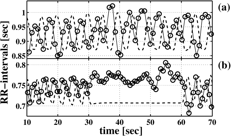
Figure 1: $RR$-intervals for (a) normal (spontaneous) and (b) intermittent respirations. Respiration signals (arbitrary units) are shown by dashed lines.

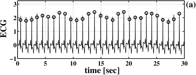
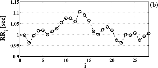
Figure 2: (a) An ECG signal and (b) the corresponding HRV ($RR$ intervals) signal. In (a) the R-peaks are marked by $\opencircle$; the ECG signal is shown in arbitrary units.

Consideration of the intrinsic activity of the heart control system on short-time scales is important for general understanding of the function of the cardio-vascular system, leads potentially to diagnostics of causes of arrhythmia involving problems with neuronal control [20], and can be a benchmark for modeling HRV. In this paper we present the results of an experimental study of the intrinsic dynamics of the heart regulatory system and discuss these results in the context of modelling the fast noise component. A number of open problems are identified.

2 Experimental results

We analyse the dynamics of the control system in the absence of explicit perturbations by temporarily removing the continuing perturbations caused by respiration [figure 1(b)]. To do so, we perform experiments involving modest breath-holding (apnœa) intervals. Note that during long breath-holding the normal state of the cardiovascular system is significantly modified [21]. The idea of the experiments came from the observation that spontaneous apnœa occurs during repose. Apnœa intervals of up to 30 sec were used, enabling us to avoid either anoxia or hyper-ventilation [21].

Respiration-free intervals were produced by intermittent respiration, involving an alternation between several normal (non-deep) breaths and then a breath-hold following the last expiration, as indicated by the dashed line in figure 1(b). The respiratory amplitude was kept close to normal to avoid hyper-ventilation, and there were relatively long intervals of apnœa when the heart dynamics was not perturbed by respiration. It is precisely these intervals that are our main object of analysis. The durations of both respiration and apnœa intervals were fixed at 30 sec.

Measurements were carried out for 5 relaxed supine subjects, and they were approved by Research Ethics Committee of Lancaster University. Note that the measurements presented have been selected from a larger number of measurements to form a set recorded under almost identical conditions of time and duration, with the subjects avoiding either coffee or a meal for at least 2 hours beforehand. They were 4 males and 1 female, aged in the range 29–36 years, non-smokers, without any history of heart disease. We stress that the aim of the current investigation was exploratory: to study typical behaviour of the internal regulatory system; we have not performed a large-scale trial of the kind widely used in medicine when a large number of subjects is necessary because of the need for subsequent statistical analysis of the data. The electrocardiogram (ECG) and respiration signals were recorded [17] over 45-60 minutes. The ECG signals were transformed to HRV by using the marked events method for extraction of the $RR$-intervals which are shown in figure 2.

Figure 1 shows $RR$-intervals found for the different types of respiration. It is evident that respiration changes the heart rhythm very significantly. Immediately after exhalation (b), there is an apnœa interval where the heart rhythm fluctuates around some level. These fluctuations correspond to the intrinsic dynamics of the heart control system. It is clear from (a) that heart rate is continuously perturbed during normal respiration, whereas in (b) one can distinguish an interval of intrinsic dynamics corresponding to apnœa. Thus, the $j$th interval of apnœa is characterized by the time series $\{RR_{i}\}$; here $i=1,2\ldots$ labels the $i$th $RR$-interval. Finally, we form a set $\{RR_{i}\}^{j}$ for analyses by considering the set as realizations of a random walk and analyzing their dynamical properties as such.

To reveal dynamics additional to $RR$-intervals, the differential increments $\Delta RR_{i}=RR_{i+1}-RR_{i}$ were analyzed. The differences between $RR$-intervals and their increments are illustrated in figure 3. Each apnœa time-series $\{RR_{i}\}^{j}$ exhibits a trend that is describable by the slope $a$ of a linear function $RR^{j}_{i}\propto a_{j}\,i$, where $i$ is a heart beat number and $j$ marks $j$th apnœa interval. The trend can be characterized by the distribution of slopes $P(a)$ shown in figure 4 (a). For all measurements the distributions are broad and their mean values differ from zero. Thus the non-stationary nature of HRV on short time-scales is clearly apparent. Note, that the distributions $p(a)$ for the increments $\Delta RR$ are significantly narrower [figure 4 (b)] and that they are very well fitted to a normal distribution; however, the mean values of the slopes differ from zero.

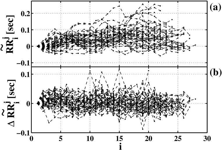
Figure 3: (a) $RR$-intervals and (b) increments $\Delta RR$ corresponding to apnœa intervals are shown. For convenience of presentation, the difference between a given value and the first value of each $j$th apnœa interval is drawn in each case: $\widetilde{RR}_{i}^{j}=RR_{i}^{j}-RR_{1}^{j}$ and $\Delta\widetilde{RR}_{i}^{j}=\Delta RR_{i}^{j}-\Delta RR_{1}^{j}$.

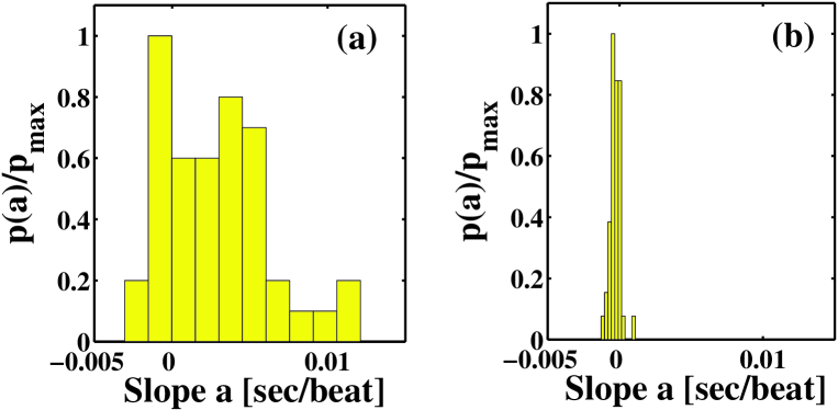
Figure 4: Distributions of trend slopes $P(a)$ of the sets (a) $\{RR_{i}\}^{j}$ and (b) $\{\Delta RR_{i}\}^{j}$.

Because the dynamics of $RR$-intervals is evidently non-stationary, we have applied detrended fluctuation analysis (DFA) [10] for estimation of the scaling exponents $\beta$ for the apnœa sets $\{RR_{i}\}^{j}$. In doing so, we adapted the DFA method [10] for short time-series and used non-overlapped windows (see Appendix for details). Because the time-series were short, time windows of length 4–15 $RR$-intervals were used to calculate $\beta$. For all measured subjects, this procedure yielded values of $\beta$ lying within the range $\beta\in(1.3:1.7)$, with a mean value of $1.45$. If $RR$-intervals in the sets $\{RR_{i}\}^{j}$ are replaced by realizations of Brown noise (the integral of white noise) keeping same lengths of apnœa intervals, then the calculation gives $\beta=1.46\pm 0.07$. Additionally, a surrogate analysis was performed for each subject by random shuffling of the time indices $i$ of $RR_{i}$-intervals, to confirm the importance of time-ordering of the $RR$-intervals. For each realization (set $\{RR_{i}\}^{j}$), 100 surrogate sets were generated, 100 values of $\beta$ were obtained, and the mean value $\beta_{s}$ was calculated. Values of $\beta_{s}$ for the surrogate sets lie in the same limits as those for the original sets, but with a small bias between $\beta$, calculated using original sets, and $\beta_{s}$ (see the Appendix for values of $\beta$ and $\beta_{s}$). It means that one can see a correlation between $RR$-intervals, but that it is weak. Summarizing the DFA results, we can claim that the scaling exponent $\beta$ is similar to that for free diffusion of a Brownian particle, but there is nonetheless some correlation between the $RR$-intervals. We also applied aggregation analysis [19] in a similar manner and arrived at qualitatively the same conclusion. Note that in the contrast to the initial idea of the DFA and aggregation analyses, which were used for revealing long-range correlations in time series, we have used these approaches to analyse the diffusion velocity because they can cope with trends. Long-range correlations cannot be revealed in the described measurements.

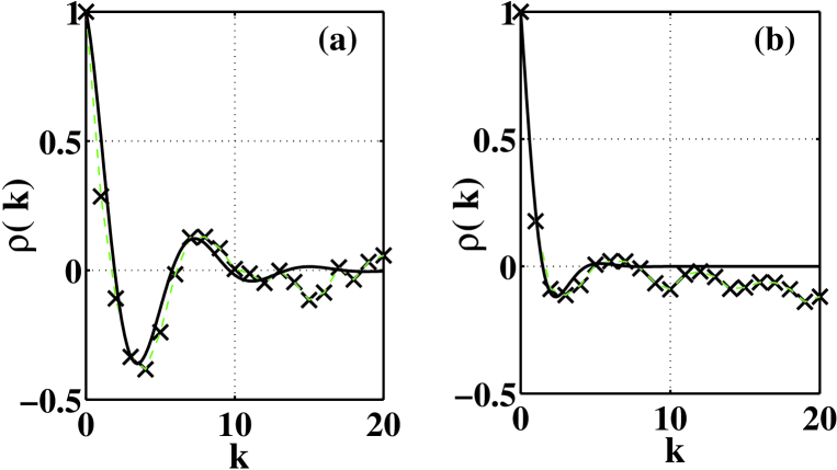
Figure 5: Examples of the autocorrelation function $\rho(k)$ (a) with and (b) without an oscillatory component. The crosses indicate $\rho(k)$ calculated on the basis of the increments $\Delta RR$. The solid line corresponds to the approximating curve $\rho^{a}(k)=\exp(-\gamma k)\cos(2\pi\Omega k)$.

To estimate the strength of the correlation, stationary time-series of the increments $\{\Delta RR_{i}\}^{j}$ were considered. The autocorrelation function $\rho(k)$ was calculated

$$\rho(k)=\frac{1}{(M-1)\sigma}\sum_{j=1}^{N}\sum_{i=1}^{m^{j}-k}\widehat{RR}_{i}^{j}\widehat{RR}_{i-k}^{j};$$ (1)

$$M=\sum_{j=1}^{N}(m_{j}-k),\ \ \ \ \ \ \ \ \ \ \sigma=\frac{1}{M-1}\sum_{j=1}^{N}\sum_{i=1}^{m^{j}-k}\left(\widehat{RR}_{i}^{j}\right)^{2}.$$

Here $\widehat{RR}_{i}^{j}=\Delta RR_{i}^{j}-\langle\Delta RR^{j}\rangle$; the brackets $\langle\rangle$ denote calculation of the mean value; $i$ and $j$ correspond to the heart beat number and apnœa interval respectively, $k=0,1,\ldots$, $m^{j}$ is the number of increments $\Delta RR$ in the $j^{\rm th}$ apnœa; $N$ is the total number of apnœa intervals. Figure 5 presents examples of autocorrelation functions. One of them has pronounced oscillations. An approximation of $\rho(k)$ by the function $\rho^{a}(k)=\exp(-\gamma k)\cos(2\pi\Omega k)$ demonstrates that oscillations occur with frequency near $0.1$ Hz, presumably corresponding to myogenic processes [17] or (perhaps equivalently) to the Mayer wave associated with blood pressure feedback [22, 23]. Further investigations via the parametrical spectral analysis for each apnœa interval show that these oscillations are of an on-off nature, i.e. observed for parts of the apnœa intervals, and not in all of the measurements as can be seen in figure 5 (b). Examples of apnœa intervals with and without oscillations are shown in figure 6. When an oscillatory component is present then its contribution to $\rho(k)$ is much weaker than the contribution of the noisy component. The latter is characterized by a very short memory as demonstrated by fast decay of $\rho(k)$.

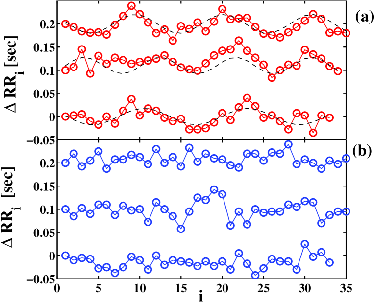
Figure 6: Examples of apnœa intervals with (a) and without (b) oscillation of HRV. The circles correspond to the values of the increments $\Delta RR_{i}$ and the solid lines connecting points are guides to the eye. The dashed lines in figure (a) are added to reveal oscillations. The middle and upper $\Delta RR_{i}$ time-series are shifted by 0.1 and 0.2 (sec) accordingly.

The properties of $\Delta RR$ can also be characterized by the probability density function $P(\Delta RR)$ shown in figure 7 (a). Figure (b) shows the probability density function $P(RR)$ of RR-intervals for comparison. Following [24], the $\alpha$-stable distribution has been widely used to fit the distribution of increments $\Delta RR$, and strongly non-Gaussian distributions were observed [24]. We perform a similar fitting applying special software [25]. Since the distributions $P(\Delta RR)$ are almost symmetrical, our attention was concentrated on the tails, which were characterized by a stability index $\alpha\in(0,2]$. The case of $\alpha=2$ corresponds to a Gaussian and, if $\alpha<2$, the tails are wider than Gaussian. Fitting to our results yields a stability index $\alpha\in(1.8:2)$, and the goodness-of-fit test (modified KS-test taking into account the weight to the tails [25]) supports the fitting. Note that, although the autocorrelation function $\rho(k)$ cannot be used for the theoretical description of an $\alpha$-stable process [26], $\rho(k)$ is nonetheless applicable for finite time-series.

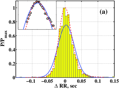
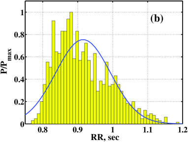
Figure 7: (Color online) Normalized probability density functions (a) $P(\Delta RR)$ of increments of $RR$-intervals and (b) $P(RR)$ of $RR$-intervals. In (a) the full (blue) and dashed (red) lines are Gaussian and stable distributions, respectively, fitted to the data. The insets show the same distributions plotted with logarithmic ordinate scales; the circles correspond to $P(\Delta RR)$. The stable distribution in (a) is characterized by $\alpha=1.86$. In (b) the full (blue) line is a Gaussian distribution fitted to the data.

If we consider the same length of realization using a Gaussian random variable instead, we find $\alpha=1.99\pm 0.01$. It means that the calculations of $\alpha$ are very robust. In addition we carried out a stability test and it too supported the fitting results. The obtained values of $\alpha\in(1.8:2)$ differ significantly from the previously reported values $\alpha\in(1.5:1.7)$ for 24h time-series of $RR$-intervals [24].

Combining all the results, we conclude that the short-time dynamics of $RR$-intervals can be described as a stochastic process with stationary increments. This type of stochastic processes was discussed by A. N. Kolmogorov [27] and applied to the description of a number of different problems (see e.g. [28, 29, 30] for further details). So, HRV during apnœa interval cab be presented in the following form

$$RR_{i}=RR_{i-1}+\Delta RR_{i},$$ (2)

where $\Delta RR_{i}$ is a stationary discrete time stochastic process. Note that the DFA calculation excludes a linear trend, which is taken into account in Eq. (2) as non-zero mean value of the increments, $\mu_{j}=\langle\Delta RR_{i}\rangle_{j}$; in general case, $\mu_{j}$ is a random function of $j$th apnœa interval. If one represents $RR$-intervals as a sum of the linear trend and a random component:

$$RR_{i}=\mu_{j}\,i+\xi_{i},$$ (3)

then $\xi_{i}$ corresponds to the non-stationary process (2) with zero mean value of increments. In other words, the superimposed random component of HRV during apnœa intervals is described by a non-stationary random process.

Increments $\Delta RR_{i}$ are characterized by a random $\alpha$-stable process of short memory, with a weak intermittent oscillatory component of frequency $\sim$ 0.1 Hz. In the zeroth approximation the increments can safely be represented by an uncorrelated Gaussian random process but, in the next approximation, a weak correlation must be included, allowing for an intermittent oscillatory component, and for weak non-Gaussianity of the distribution of increments $\Delta RR$. These additions reveal, on the one hand, that the previously reported observation of a non-Gaussian distribution of increments [24] is a property of the intrinsic heart rate regulatory system, but on the other hand, that the scaling ranges of the stability index $\alpha$ differ significantly in the presence or absence of external perturbations (including respiration) acting on the regulatory system. Consequently an explanation of the scalings reported in [24, 10] should include analyses of the effect of external perturbations and respiration, and not an analysis of heart rate alone.

3 Discussion

3.1 Non-stationarity of $RR$-intervals during apnoea

The results presented indicate that there is no firm set point for the heart control system, and that the heart rhythm exhibits diffusive behaviour. The slowest dynamics can be described by a linear trend during apnœa intervals and its presence can be treated as a slow regulatory/adaptation component of the control system. The presence of the slow time-scales is an established property of HRV [31] and their presence, even in the absence of the respiratory perturbation, can be interpreted as an expected property.

On short time-scales of order several seconds, HRV shows a diffusive dynamics too. It can be interpreted in two ways. One possibility is that the control system does not firmly trace the base (slow) rhythm, because in case of tracing, short time-fluctuations should “jump” around the base rhythm and, consequently, be stationary. Such a picture corresponds to zero action of the control system if the heart rate is in a “safe” (for the whole cardiovascular system) interval, e.g. $RR\in[RR_{low}:RR_{high}]$. Another possible explanation could be that the control system is tracing the base rhythm but the short-time fluctuations have a non-stationary character. It is natural to expect that there could be other possible explanations, and additional investigations are needed to reach an understanding of the diffusive dynamics on short-time scales.

In section 2 it is suggested that we should consider the non-stationarity and diffusive dynamics of $RR$-intervals within the framework of a stochastic process with independent increments. It allows one to consider $RR$-intervals as realizations of the so-called auto-regressive process that is widely used in time-series analysis [32]. It means that the direct spectral estimation of $RR$-intervals, currently used as one of the basic techniques [31], is not applicable here and that one must use the theory of stochastic processes with stationary increments for their spectral decomposition [30]. If in the presence of respiration, the short-time stochastic component of HRV preserves non-stationarity then spectral estimation based on $RR$-intervals is not correct, and increments must be used instead. Note, that the properties of short-time fluctuations in the presence of respiration are far from being completely understood.

3.2 Non-Gaussianity and correlations of increments $\Delta RR$

The theories of both stochastic processes with stationary increments and of auto-regressive analysis place some limitations on the analysed time-series. The first approach requires the existence of finite second-order momenta, whereas the second approach assumes uncorrelated statistics of increments. Formally, however, non-Gaussianity of the increments distribution means that the second-order momenta do not exist [26], but non-Gaussianity can still be incorporated into the auto-regressive description [33]. And vice versa, the presence of correlations in the increments dynamics requires a modification of the standard auto-regressive approach, and it is one that can be incorporated naturally into the general theory. In the current investigation we ignore these issues. We calculate the auto-correlation function and use model (2), because the finite length of the time-series guarantees the existence of the second-order momenta, and the simplicity of (2) means that the inclusion of the correlations is a trivial extension.

Our consideration has the formal character of time-series analysis because we do not incorporate any preliminary information about the possible dynamics of $RR$-intervals. The analysis is based on the use of a set of relatively short time-series, a fact that defines our choice of simple statistical measures. One cannot exclude the possibility that the use of other approaches to such data might provide additional insight into HRV dynamics. For example, the fractional Brownian motion approach [19, 34] and the theory of discrete non-stationary non-Markov random process [35] represent different paradigms, which are based on assumptions about the origin of the data. Note, that despite a long history of developing the approaches and their applications, the approaches of fractional Brownian motion and of stable random process are not standardized tools, whereas the approach of non-Markov random process is not so popular. There is no definite recipe for choosing a set of measures which can uniquely specify (or provide a good description of) the properties of a renewal (discrete time) stochastic process.

3.3 Modelling

Another way of attempting to understand the results is to try to reproduce the observed data properties from an appropriate model. In the context of our experiments, the modelling should consist of a simulation of the electrical activity of sinoatrial node (SAN) where the heart beats are initiated. For modelling, one option is to use a bottom-up approach, which is currently a very popular technique within the framework of the complexity paradigm. In fact, available SAN cellular models allow one to incorporate many details of physiological processes like the openings and closures of specific ion channels [36]. However, despite the complexity of the models (40–100 variables) many important features are still missed. For example, the fundamentally stochastic dynamics of ion channels is represented by equations that are deterministic. Heterogeneity of the SAN cellular locations and intercell communications are among other important open issues [37, 38].

An alternative option is the top-down approach using integrative phenomenological models. In contrast to detailed cell models, a toy model of the heart as a whole unit can be developed. It is known that an isolated heart, and a heart in the case of a brain-dead patient [39] demonstrate nearly periodic behaviour. So, it is reasonable to assume that the observed HRV is induced by the neuronal heart control system, which is a part of the central nervous system. The control system includes a primary site for regulation located in the medulla [40], consisting of a set of neural networks with connections to the hypothalamus and the cortex. The control is realized via two branches of the nervous system: the parasympathetic (vagal) and the sympathetic branches. Although many details of the control system are still missing [41, 20], it is currently accepted that the vagal branch operates on faster time scales than the sympathetic one, and that each branch has a specific co-operative action on the heart rate and the dynamics of SAN cells.

Let us consider an integrate-and-fire (IF) model as a model of a SAN cell in the leading pacemaker. These cells are responsible for initiating the activity of SAN cells and, consequently, that of the whole heart [38]. The dynamics of the IF model describes the membrane potential $U(t)$ of the cell by the following equations

$$\frac{dU}{dt}=\frac{1}{\tau}~{}~{}~{}~{}~{}~{}~{}~{}~{}~{}~{}~{}~{}~{}~{}~{}~{}~{}~{}~{}~{} \mbox{if}\ \ \ U(t)<U_{t}$$ (4)

$$U(t)=U_{r},\ \ t^{*}=t \mbox{if}\ \ \ U(t)=U_{t}\ \ \ \mbox{and}\ \ \ \frac{dU}{dt}>0,$$ (5)

Here $1/\tau$ defines a slope of integration, $U_{t}$ is the threshold potential, $U_{r}$ is the resting (hyperpolarization) potential; the time $t^{*}$ corresponds to the cell firing, and it is the difference between two successive firings that determines the instantaneous heart period or $RR$-interval, $RR_{i}=t^{*}_{i}-t^{*}_{i-1}$. It is known [40] that increasing sympathetic activity with a combination of decreasing vagal activity leads to an increase in the heart period, and vice versa. Direct stimulation of the sympathetic branch leads to an increase of the integration slope $1/\tau$ and a lowering of the threshold potential $U_{t}$, whereas vagal activation has the opposite effects, and additionally, lowers the resting potential $U_{r}$. Thus, the neuronal activities can be taken into account as modulations of the parameters of the IF model (4). For reproducing HRV during apnœa, therefore, it is enough to present any of the parameters $\tau$, $U_{t}$ or $U_{r}$ as a stochastic variable of the form (2), for example, $U_{t}(t^{*}_{i})=U_{t}(t^{*}_{i-1})+\xi_{i}$, where $\xi_{i}$ are random numbers having the stable distribution.

However, the use of more realistic (than IF) models with oscillatory dynamics, for example Fitzhugh-Nagumo [42] or Morris-Lecar [43] models, makes the reproduction of the experimental results a more difficult but interesting task. Currently it is unclear whether it is possible to obtain a stable distribution of increments by consideration of the Gaussian type of fluctuations alone, or whether one should use fluctuations characterizing by a stable distribution. This point demands further investigation.

4 Conclusion

In summary, our experimental modification of the respiration process reveals that the intrinsic dynamics of the heart rate regulatory system exhibits stochastic features and can be viewed as the integrated action of many weakly interacting components. Even on a short time scale (less then half a minute) the heart rate is non-stationary and exhibits diffusive dynamics with superimposed intermittent $\sim$ 0.1 Hz oscillations. The intrinsic dynamics can be described as a stochastic process with independent increments and can be understood within the framework of many-body dynamics as used in statistical physics. The large number of independent regulatory perturbations produce a noisy regulatory background, so that the dynamics of the regulatory rhythm is close to classical Brownian motion. However there are indications of non-Gaussianity of increments and weak but important correlations on short time-scales. The reproduction of these features, especially the non-Gaussianity property, is an open problem even in simple toy models.

These results are important both for understanding the general principles of regulation in biological systems, and for modeling cardiovascular dynamics. Furthermore, the results presented may possibly lead to a new clinical classification of states of the cardiovascular system by analysing the intrinsic dynamics of the heart control system as suggested in [20].

Appendix

Some details of the measurements and calculations are summarized in this section.

The ECG was measured by standard limb (Einthoven) leads and the respiration signal was measured by a thoracic strain gauge transducer. The signals were digitized by a 16-bit analog-to-digital converter with a sampling rate of 2 kHz. The ECG and respiration signals were recorded over 45-60 minutes and time locations of $R$-peaks in the ECG signals were defined and time intervals between two subsequent $R$-peaks (the so called $RR$-intervals) are used to form HRV signal.

Respiration-free intervals were produced by the intermittent respiration, involving an alternation between normal breaths and apnœa intervals. The durations of both normal breaths and apnœa intervals were fixed at 30 sec. The respiration signal was used to identify apnœa intervals. Finally, the set of time-series of $RR$-interval $\{RR_{i}\}^{j}$ was formed for each subject; here $i=1,2\ldots$ labels the $i$th $RR$-intervals, and $j=1,2\ldots$ labels the $j$th interval of apnœa. For each interval of apnoea, time series of the differential increments $\Delta RR_{i}=RR_{i+1}-RR_{i}$ were produced and they also form a set $\{\Delta RR_{i}\}^{j}$ for each subject. The number of $RR$-intervals in each apnœa interval is different, depending on the heart rate of the subject. The total number of apnœa intervals also differ for each subject. The mean heart rate $\langle RR\rangle$ during apnœa intervals and the total number $J$ of intervals for each measured subject are presented in table 1.

Table 1: Data for each subject. $\langle RR\rangle$ is the mean heart rate during apnœa. $J$ is the total number of apnœa intervals. $\beta$ is the DFA scaling exponent calculated for the apnœa set $\{RR_{i}\}^{j}$. $\beta_{s}$ is the mean value of the DFA scaling exponent calculated for surrogate data, which were generated by random shuffling of the time indices $i$ of $RR_{i}$-intervals. $b$ is the scaling exponent of the aggregation analysis. $\gamma$ and $\Omega$ correspond to the values of parameters for the function $\rho^{a}(k)=\exp(-\gamma k)\cos(2\pi\Omega k)$ which approximates the autocorrelation function $\rho(k)$. $\alpha$ is the stability index of the distribution $P(\Delta RR)$.

• Subject	$\langle RR\rangle$ (sec)	$J$	$\beta$	$\beta_{s}$	$b$	$\gamma$	$\Omega$	$\alpha$
  S1	1.01	45	1.39	1.47	1.86	0.81	0.17	1.83
  S2	0.77	46	1.46	1.44	1.83	0.21	0.09	1.95
  S3	1.10	47	1.43	1.53	1.96	1.01	0.22	1.79
  S4	0.75	47	1.58	1.60	1.91	0.15	0.08	1.90
  S5	0.91	60	1.42	1.48	1.82	0.28	0.13	1.86

For the application of the DFA and aggregation analyses we adapted the approaches described in [10] and [19], respectively, to treat the available sets of short time series $\{RR_{i}\}^{j}$.

The DFA exponent $\beta$ was calculated in the following way. First, the initial set $\{RR_{i}\}^{j}$ was transformed to another set $\{y(k)\}^{j}$ by the following expression:

$$y(k)=\sum_{i=1}^{k}RR_{i},$$ (6)

where $k=1\ldots M_{j}$ and $M_{j}$ is the number of $RR$-intervals for $j$th apnoea interval. For each length $n=4,\ldots 15$ of time window a set of linear trends $\{y^{n}(k)\}^{j}$ was calculated (see [10] for details), where $y^{n}(k)=k\cdot a_{m}^{n}+b_{m}^{n}$, $m=1,\ldots\lfloor{M_{j}/n}\rfloor$, $\lfloor x\rfloor=\max\{n\in{\mathbb{Z}}|n\leq x\}$ is the floor function of $x$. Then a set of scaling function $\{\tilde{F}(n)\}^{j}$ was calculated for each value of $n$ by use of the expression

$$\tilde{F}(n)=\sum_{k}^{N_{j}}[y(k)-y^{n}(k)]^{2},$$ (7)

where $N_{j}=\lfloor{M_{j}/n}\rfloor\cdot n$. Further the scaling functions $F(n)$ were calculated as

$$F(n)=\sqrt{\frac{1}{N-1}\sum_{j=1}^{J}\tilde{F}_{j}(n)},$$ (8)

where $J$ is the number of apnoea intervals for the given subject, $N=\sum_{j=1}^{J}N_{j}$. Finally, the scaling exponent $\beta$ was determined as a slope of the function $\log[F(n)]\propto\beta\log(n)$ (see figure 8 (a)). The values of $\beta$ for the different subjects are shown in table 1.

The aggregation analysis consists of three steps and the final result is the scaling exponent $b$. The first step is the creation of a set of aggregated time series $\{z_{m}(k)\}^{j}$ for different $m=1,\ldots 10$:

$$z_{m}(k)=\sum_{i=k}^{k+m}RR_{i},$$ (9)

where $k=1,\ldots M_{j}-m$. Then a realization $z_{m}(k)$ was formed from the set $\{z_{m}(k)\}^{j}$: $z_{m}(k)=\{z_{m}(k)\}^{j}=\{z_{m}(k)\}^{1},\ldots\{z_{m}(k)\}^{J}$. The second step includes the calculation of the mean value $\mu(m)$ and variance $\sigma(m)$ of the time-series $z_{m}(k)$:

$$\mu(m)=\frac{1}{M}\sum_{k=1}^{M}z_{m}(k),\ \ \ \ \sigma(m)=\frac{1}{M-1}\sum_{k=1}^{M}\left[z_{m}(k)-\mu(m)\right]^{2},$$ (10)

where $M$ is the whole length of time series $z_{m}(k)$. The slope $b$ of the function $\log[\sigma(m)]\propto b\log[\mu(m)]$ was calculated in the third step (see figure 8 (b)). The values of $b$ for each subject are shown in table 1.

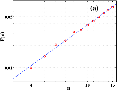
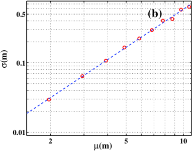
Figure 8: (a) The scaling function $F(n)$ (circles) and its approximation (dashed line) by $F(n)\propto n^{\beta}$ ($\beta=1.39$) are shown. (b) The dependence (circles) of the variance $\sigma(m)$ on the mean value $\mu(m)$ for $m=1,\ldots 10$ and its approximation (dashed line) by $\sigma(m)\propto\mu(m)^{b}$ ($b=1.82$) are shown.

To verify the robustness of the calculations of exponents $\beta$ and $b$ we have performed calculations with the same number of RR-intervals as well as the same structure of apnœa intervals but by using realizations of Brown noise generated by computer. In other words, in the procedures described above we replaced $\{RR_{i}\}^{j}$ by $\{W_{i}\}^{j}$, where $W_{i}=W_{i-1}+0.2\cdot\xi_{i}$ for $i=2,\cdots M_{j}$, $W_{1}=RR_{1}$, and $\xi_{i}$ are random numbers having the normal distribution with mean zero value and unit variance; the numbers $\xi_{i}$ are different for different $j$th intervals of apnœa. We performed 100 calculation of $\beta$ and $b$ for different sets $\{W_{i}\}^{j}$ for each subject. Theoretical values of $\beta$ and $b$ for the Brown noise are $\beta=1.5$ and $b=2$ correspondingly. The calculations with Brown noise gave $\beta=1.46\pm 0.07$ and $b=1.84\pm 0.04$. Here data were merged for all subjects and are presented in the form of a mean value $\pm$ its standard deviation. It means that there is a systematic error related to the length and data structure, a general error of calculation in respect to the theoretical values for $\beta$ is $~{}1.5$ and for $b$ is $~{}2.0$. However the standard deviations of the calculated values are rather small and, consequently, we can conclude that our calculations of $\beta$ and $b$ are robust.

References

References

- [1] Ott E 1993 Chaos in Dynamical Systems (Cambridge, UK: Cambridge University Press)
- [2] Frisch U 1995 Turbulence: The Legacy of A.N. Kolmogorov (Cambridge, UK: Cambridge University Press)
- [3] Mandelbrot B B 1982 The Fractal Geometry of Nature (W. H. Freeman)
- [4] Jensen H J 1998 Self-Organized Criticality: Emergent Complex Behavior in Physical and Biological Systems (Cambridge, UK: Cambridge University Press)
- [5] Kurths J, Voss A, Saparin P, Witt A, Kleiner H J and Wessel N 1995 Chaos 5(1) 88–94
- [6] Pincus S M 1991 Proc. Nat. Acad. Sci. 88(6) 2297–2301
- [7] Costa M, Goldberger A L and Peng C K 2002 Phys. Rev. Lett. 89(6) 068102
- [8] Raab C, Wessel N, Schirdewan A and Kurths J 2006 Phys. Rev. E 73(4) 041907
- [9] Kiyono K, Struzik Z R, Aoyagi N, Togo F and Yamamoto Y 2005 Phys. Rev. Lett. 95(5) 058101
- [10] Peng C K, Havlin S, Stanley H E and Goldberger A L 1995 Chaos 5(1) 82–87
- [11] Hausdorff J M and Peng C K 1996 Phys. Rev. E 54(2) 2154–2157
- [12] Pilgram B and Kaplan D T 1999 Amer. J. of Physiol. – Regulatory, Integrative and Comparative Physiol 276(1) R1–R9
- [13] Costa M, Goldberger A L and Peng C K 2005 Phys. Rev. Lett. 95 198102
- [14] Ivanov P C, Amaral L A N, Goldberger A L, Havlin S, Rosenblum M G, Struzik Z R and Stanley H E 1999 Nature 399(6735) 461–465
- [15] Ivanov P C, Amaral L A N, Goldberger A L, Havlin S, M G Rosenblum H E S and Struzik Z R 2001 Chaos 11(3) 641–652
- [16] Ivanov P C, Amaral L A N, Goldberger A L and Stanley H E 1998 Europhys. Lett. 43(4) 363–368
- [17] Stefanovska A and Bračič M 1999 Contemporary Phys. 40(1) 31–55
- [18] Eckberg D L 2003 J. Physiol. (Lond.) 548(2) 339–352
- [19] West B J, Griffin L A, Frederick H J and Moon R E 2005 Resp. Physiol. and Neurobiol. 145(2-3) 219–233
- [20] Doessel O, Reumann M, Seemann G and Weiss D 2006 Biomedizinische Technik 51(4) 205–209
- [21] Parkes M J 2006 Exper. Physiol. 91(1) 1–15
- [22] Malpas S C 2002 Am. J. Physiol.: Heart. Circ. Physiol. 282 H6–H20
- [23] Julien C 2006 J. Appl. Physiol. 101(2) 684
- [24] Peng C K, Mietus J, Hausdorff J M, Havlin S, Stanley H E and Goldberger A L 1993 Phys. Rev. Lett. 70(9) 1343–1346
- [25] Nolan J P 1998 Stat. and Probabil. Lett. 38(2) 187–195
- [26] Samorodnitsky G and Taqqu M S 1994 Stable Non-Gaussian Random Processes: Stochastic Models with Infinite Variance (London, UK: Chapman and Hall)
- [27] Kolmogorov A N 1940 Doklady Akademii Nauk SSSR 26(1) 6–9
- [28] Doob J L 1990 Stochastic Processes (New York: Wiley-Interscience)
- [29] Yaglom A M 1962 An Introduction to the Theory of Stationary Random Functions (Englewood Cliffs, NJ.: Prentice-Hall)
- [30] Rytov S M, Kravtsov Y A and Tatarskii V I 1988 Principles of Statistical Radiophysics vol 2: Correlation Theory of Random Processes (Springer-Verlag)
- [31] Camm A J, Malik M, Bigger J T and et al 1996 Circulation 93(5) 1043–1065
- [32] Box G, Jenkins G M and Reinsel G 1994 Time Series Analysis: Forecasting & Control (3rd Edn) (Englewood Cliffs, NJ: Prentice Hall)
- [33] Nikias C L and Min Shao 1995 Signal Processing with Alpha-stable Distributions and Applications (New York, NY, USA: Wiley-Interscience)
- [34] Heneghan C and McDarby G 2000 Phys. Rev. E 62(5) 6103–6110
- [35] Yulmetyev R, Hänggi P and Gafarov F 2002 Phys. Rev. E 65(4) 046107
- [36] Wilders R 2007 Med. and Biol. Eng. and Comp. 45(2) 189–207
- [37] Ponard J G C, Kondratyev A A and Kucera J P 2007 Biophys. J. 92(10) 3734–3752
- [38] Dobrzynski H, Li J, Tellez J, Greener I D, Nikolski V P, Wright S E, Parson S H, Jones S A, Lancaster M K, Yamamoto M, Honjo H, Takagishi Y, Kodama I, Efimov I R, Billeter R and Boyett M R 2005 Circulation 111(7) 846–854
- [39] Neumann T, Post H, Ganz R E, Walz M K, Skyschally A, Schulz R and Heusch G 2001 Zeitschrift für Kardiologie 90(7) 484–491
- [40] Klabunde R E 2004 Cardiovascular Physiology Concepts (Philadelphia, USA: Lippincott Williams & Wilkins)
- [41] Armour J A 2004 Amer. J. Physiol. – Regulatory Integrative and Comparative Physiol. 287(2) R262–R271
- [42] Fitzhugh R 1961 Biophys. J. 1(6) 445
- [43] Morris C and Lecar H 1981 Biophys. J. 35(1) 193–213