Fluid phase coexistence and critical behaviour from simulations in the restricted Gibbs ensemble

Abstract

The symmetrical restricted Gibbs ensemble (RGE) is a version of the Gibbs ensemble in which particles are exchanged between two boxes of fixed equal volumes. It has recently come to prominence because – when combined with specialized algorithms – it provides for the study of near-coexistence density fluctuations in highly size-asymmetric binary mixtures. Hitherto, however, a detailed framework for extracting accurate estimates of critical point and coexistence curve parameters from RGE density fluctuations has been lacking. Here we address this problem by exploiting an exact link between the RGE density fluctuations and those of the grand canonical ensemble. In the sub-critical region we propose and test a simple method for obtaining accurate estimates of coexistence densities. In the critical region we identify an observable that serves as a finite system size estimator for the critical point parameters, and present a finite-size scaling theory that allows extrapolation to the thermodynamic limit.

I Introduction

In a recent paper Liu et al LIU2006 have presented a method for studying density fluctuations in highly size-asymmetric binary fluids. The method draws on the geometrical cluster algorithm (GCA) of Liu and Luijten Liu2004_0 which facilitates rejection-free Monte Carlo simulations of highly asymmetric mixtures via large-scale collective updates which move whole groups of particles (both large and small) in a single step. In its basic form, the GCA is inherently canonical, i.e. it conserves the total number of particles in the system. To enable density fluctuations – and thus facilitate the study of phase behaviour – it was modified in ref. LIU2006 so that cluster updates transfer particles between two subsystems of fixed equal volumes, thus realizing complementary density fluctuations within each subsystem. Such a scenario constitutes a special case of the well known Gibbs ensemble (GE) PANAGIO87 , which has been dubbed the restricted Gibbs ensemble (RGE) Mon1992 ; Bruce97 due to the absence of volume transfers between the boxes. The lack of volume fluctuations in the RGE (which are incompatible with cluster updates) means that the two subsystems do not remain at equal pressure – a fact which complicates the determination of phase coexistence points.

In this paper we address the issue of how to determine coexistence curve and critical point parameters within the RGE. For simplicity we perform the analysis for a single component fluid, but we expect the results to be directly applicable to the asymmetrical binary case in which the GCA+RGE method operates . Our reference point is the well studied grand canonical ensemble (GCE) for which powerful techniques exist for determining critical points and coexistence curve properties wilding1995a . In order to develop methods of comparable utility, we appeal to an exact link between the density fluctuations in the RGE and those of the GCE. This link is exploited to predict the properties of simulations performed in the RGE simulations on the basis of data accumulated from GCE simulations. A detailed analysis shows, in particular, how one can locate criticality and the coexistence binodal within the RGE.

II Linking the restricted Gibbs and grand canonical ensembles

The symmetrical restricted Gibbs ensemble comprises two subsystems (or boxes) of fixed equal volumes $V_{1}=V_{2}=V=L^{d}$ (with $d=3$ in the simulations to be considered below) containing respective particle numbers $N_{1}$ and $N_{2}$ at some imposed temperature $T$. The boxes can exchange particles subject to the constraint that the total particle number

$$N_{1}+N_{2}=N_{0}$$ (1)

is fixed. The probability of finding such a restricted Gibbs ensemble system in a given microstate having particle numbers $N_{1,2}$ and coordinates $\{q\}_{1,2}$ is given by

$$P^{RG}(N_{1,2},\{q\}_{1,2}|N_{0},V,T)=\frac{\exp(-\beta(E_{1}+E_{2}))}{Z^{RG}(N_{0},V,T)}\;,$$ (2)

where $\beta=1/k_{B}T$ is the inverse temperature, while $E_{1,2}$ is the configurational energy of the respective boxes. From this it follows that the probability of finding the system with given $N_{1}$ (and hence prescribed $N_{2}$) is

$$P^{RG}(N_{1}|N_{0},V,T)=\frac{Z(N_{1},V,T)Z(N_{2},V,T)}{Z^{RG}(N_{0},V,T)}\>,$$ (3)

where $Z(N,V,T)$ is the canonical partition function.

Now to forge the link to the grand canonical ensemble, we note that

$$P(N|\mu,V,T)=\frac{Z(N,V,T)\exp(\mu N/kT)}{Z(\mu,V,T)}\>,$$ (4)

where $P(N|\mu,V,T)$ is the grand canonical probability distribution at chemical potential $\mu$. Inserting into eq. (3) yields

$$P^{RG}(N_{1}|N_{0},V,T)=wP(N_{1}|\mu,V,T)P(N_{2}|\mu,V,T)$$ (5)

where the transformation is defined for all $N_{1}\leq N_{0}$ and the normalization constant, $w$, is given by

$$w=\frac{\left[Z(\mu,V,T)\right]^{2}\exp(-\beta\mu N_{0})}{Z^{RG}(N_{0},V,T)}\>.$$ (6)

Eq. (5) is formally exact and provides the necessary link between the grand canonical and symmetrical restricted Gibbs ensembles . An interesting property of $P^{RG}$ is its independence of the choice of the chemical potential appearing on the right hand side of Eq. (5)– a feature that has its origin in the complementarity of the fluctuations of $P(N_{1})$ and $P(N_{0}-N_{1})$ .

Of course, it is more conventional to work with the number density rather than the particle number, in which case the transformation takes the form

$$P^{RG}_{L}(\rho|\rho_{0},T)\cong P_{L}(\rho|T)P_{L}(2\rho_{0}-\rho|T)\>,$$ (7)

where $\rho=N_{1}/V$ is the single box density, $P_{L}(\rho|T)$ is its GCE distribution at temperature $T$, $\rho_{0}=N_{0}/2V$ is the fixed overall density in the RGE, and $\cong$ means to within an unspecified normalization constant. For clarity we have suppressed reference to the arbitrary chemical potential $\mu$ and the constant volume $V$, but have added a subscript $L$ to emphasize that we nevertheless remain concerned with systems of finite size.

A central feature of $P^{RG}_{L}(\rho)$ is its symmetry: the transformation (7) involves the product of $P_{L}(\rho)$ and a reflected and shifted (by $2\rho_{0}$) version of itself. Quite generally [and irrespective of the symmetry of $P_{L}(\rho)$], this implies that $P^{RG}_{L}(\rho)$ is symmetric (i.e. even) with a mean value of $\rho_{0}$. This symmetry (and the $\mu$ independence of $P^{RG}_{L}(\rho)$ that it implies) precludes deployment of the standard tools for locating phase coexistence and criticality that have been developed in the context of the GCE wilding1995a . Instead bespoke analysis techniques are called for.

In this paper we develop such techniques. Perhaps surprisingly, our strategy does not involve performing actual RGE simulations. Instead we apply the exact transformation Eq. (7) to independently obtained GCE density distributions for the Lennard-Jones fluid in order to infer the properties of the resulting RGE density distribution. Our rationale for so doing is that it is well understood how one determines coexistence and critical point properties from GCE density distributions. By starting from such, we have a known baseline with which to compare the results of our analysis of the RGE. Accordingly, within this approach, GCE distributions serve as input to Eq. (7) and $\rho_{0}$ simply becomes a parameter of the transformation. As it is varied, for some prescribed $T$, a spectrum of symmetrical distributions $P^{RG}_{L}(\rho|\rho_{0})$ is generated, each centred on the respective value of $\rho_{0}$. In section IV we consider the nature of this spectrum for state points in the neighbourhood of liquid-vapor coexistence and present a method for extracting coexistence densities. Thereafter, in section V, we consider state points in the vicinity of the liquid-vapor critical point, and perform a finite-size scaling analysis of $P^{RG}_{L}(\rho)$ which facilitates accurate estimates of critical point parameters. To begin with, however, we shall briefly introduce our model system.

III Fluid model

The GCE density distributions for use as input to the transformation (7) were obtained via Monte Carlo simulations frenkelsmit2002 of a 3d fluid interacting via a Lennard-Jones (LJ) potential:

$$\phi(r)=4\epsilon[(\sigma/r)^{12}-(\sigma/r)^{6}].$$ (8)

Here $r$ is the particle separation, $\sigma$ sets the length scale and $\epsilon$ is the well depth. The potential was truncated at $r_{c}=2.5\sigma$ and no correction applied, thus allowing comparison with the results of a previous study performed under the same conditions wilding1995a . As is customary, we shall refer to the reduced temperature $T\equiv 1/(\beta\epsilon)$ rather than the well depth in the simulation results to be described below. Furthermore, we shall normally express temperature as a multiple of the critical value $T_{c}=1.1878(2)$ (as determined in Sec. V). Further details of the simulation methodology can be found in ref. wilding1995a .

For the studies of the subcritical region described in Sec. IV, a single periodic system of size $L=10\sigma$ was employed. The finite-size scaling investigation of the critical region, described in Sec. V used seven periodic systems of linear extent $L=10\sigma,\ 12.5\sigma,\ 15\sigma,\ 17.5\sigma,\ 20\sigma,\ 22.5\sigma$, $25\sigma$. We set $\sigma$ as the unit of length below.

IV Subcritical coexistence region: the intersection method

We commence by addressing the behaviour of the RGE density distributions in the subcritical coexistence region of our model fluid. As described above, our approach will be to glean information about the RGE not via explicit RGE simulations, but by applying the exact transformation Eq. (7) to GCE simulation data. Suitable estimates of the GCE density distribution $P_{L}(\rho)$ have been obtained in a previous study of the Lennard-Jones fluid by one of the authors wilding1995a . Examples for temperatures $T=0.842T_{c}$ and $T=0.69T_{c}$ are shown in Fig. 1, in which the chemical potential has been tuned so that the peaks have equal areas – the criterion for coexistence Borgs1992 .

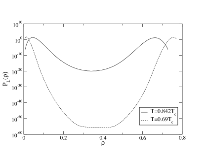
Figure 1: The form of the GCE density distribution $P_{L}(\rho)$ for temperatures $T=0.842T_{c}$ and $T=0.69T_{c}$, expressed on a logarithmic scale.

The two peaks in the coexistence form of $P_{L}(\rho)$ derive from fluctuations around the respective densities $\rho_{g}$ and $\rho_{l}$ of the gas and liquid phases. These densities are found as an average over the appropriate peak in $P_{L}(\rho)$ via

$$\ \rho_{g,l}(T)=\int_{\rho_{\mathrm{min}}}^{\rho_{\mathrm{max}}}\rho P_{L}(\rho|T)\mathrm{d}\rho\>,$$ (9)

where $\rho_{\mathrm{min}}$ and $\rho_{\mathrm{max}}$ are chosen suitably to fully encompass the appropriate peak of $P^{RG}_{L}(\rho)$, ie $\rho_{\mathrm{min}}=\rho_{g,l}-\delta$, $\rho_{\mathrm{max}}=\rho_{g,l}+\delta$. For our purposes, a useful quantity will prove to be the average of the coexistence densities at a given temperature, known as the coexistence diameter :

$$\rho_{d}(T)=[\rho_{g}(T)+\rho_{l}(T)]/2\>.$$ (10)

A pertinent feature of Fig. 1 is the shape of the distribution in the central region of density, between the peaks. Here one sees that the distribution flattens markedly, particularly so for the lower temperature. This flattening corresponds to the appearance of well defined interfaces between the coexisting phases. For sufficiently low $T$ or sufficiently large system size $L$, the central portion becomes completely flat because the interfaces decouple from one another, there being no free energy penalty for one phase to change its fractional volume with respect to the other Errington2003 .

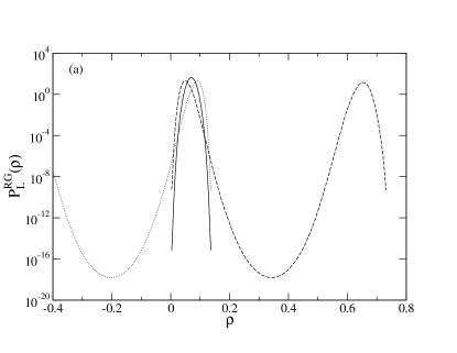
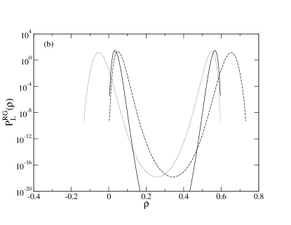
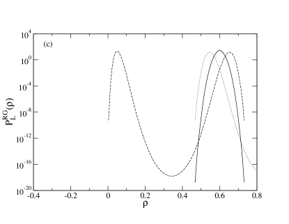
Figure 2: The form of $P^{RG}_{L}(\rho|\rho_{0})$ (expressed on a log scale) for the LJ fluid at $T=0.842T_{c}$ for (a) $\rho_{0}=0.07$; (b) $\rho_{0}=0.30$; and (c) $\rho_{0}=0.6$. In each instance the dashed curve is the coexistence form of the GCE distribution, $P_{L}(\rho)$; the dotted curve is the distribution, $P_{L}(2\rho_{0}-\rho)$, and the solid curve is the resulting RGE distribution, $P^{RG}_{L}(\rho)$ obtained via Eq. (7).

Let us now consider typical forms of $P^{RG}(\rho|\rho_{0})$ and how they derive from the underlying GCE density distribution. Examples are shown in Fig. 2 for widely separated values of $\rho_{0}$. Specifically, the figure plots the form of $P^{RG}_{L}(\rho)$ for $T=0.842T_{c}$ at three values of $\rho_{0}=0.07,0.30,0.6$. These show that for the smallest and highest values of $\rho_{0}$, $P^{RG}_{L}(\rho)$ is single peaked, while for the intermediate value of $\rho_{0}$, $P^{RG}_{L}(\rho)$ is double peaked, though in this latter case neither peak coincides with either the gas or liquid densities.

A fuller picture of the $\rho_{0}$ dependence of $P^{RG}_{L}(\rho)$ emerges by considering the peak densities as a function of $\rho_{0}$. Let us denote the densities of the low and high density peaks of $P^{RG}_{L}$ in the double-peak regime as $\rho_{-}$ and $\rho_{+}$ respectively, these being obtained as the average RGE peak density in a manner analogous to Eq. (9). A plot of $\rho_{-}$ and $\rho_{+}$ versus $\rho_{0}$ is shown in Fig. 3 for the temperature $T=0.842T_{c}$. From this figure one sees that as a function of $\rho_{0}$, the RGE distribution is single peaked at low density, splits into two peaks at intermediate $\rho_{0}$, but that these peaks merge back into a single peak at high values of $\rho_{0}$. Furthermore in the two-peak regime, $\rho_{-}$ and $\rho_{+}$ vary considerably, though we note that they remain subject to the constraint

$$\rho_{0}=(\rho_{-}+\rho_{+})/2\>,$$ (11)

which is mandated by the symmetry of $P^{RG}_{L}(\rho)$, together with the fact that its average is strictly equal to $\rho_{0}$.

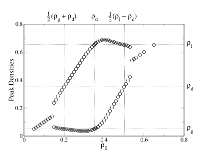
Figure 3: The peak densities of $P^{RG}_{L}(\rho)$ as a function of $\rho_{0}$ for the Lennard Jones fluid with $T=0.842T_{c}$. The dotted lines on the ordinate at low, intermediate and high densities correspond to the values of $\rho_{g}$, $\rho_{d}$ and $\rho_{l}$ respectively, as determined independently from the underlying GCE data as described in the text. The value of $\rho_{d}$ is also marked by a vertical dot-dashed line on the abscissa.

		$2\rho_{0}-\rho$
		$\rho_{g}$	$\rho_{d}$	$\rho_{l}$
$\rho$	$\rho_{g}$	$\rho_{g}$	$\frac{\rho_{g}+\rho_{d}}{2}$	$\rho_{d}$
	$\rho_{d}$	$\frac{\rho_{g}+\rho_{d}}{2}$	$\rho_{d}$	$\frac{\rho_{l}+\rho_{d}}{2}$
	$\rho_{l}$	$\rho_{d}$	$\frac{\rho_{d}+\rho_{l}}{2}$	$\rho_{l}$

Table 1: The combinations of $\rho$ (rows) and $2\rho_{0}-\rho$ (columns) corresponding to $\rho_{g},\rho_{d}$ and $\rho_{l}$. The entries in the table give the resulting $\rho_{0}$.

Now, it transpires that there are certain special values of $\rho_{0}$ for which $\rho_{-}$ and $\rho_{+}$ both coincide with one of $\rho_{g}$, $\rho_{d}$ and $\rho_{l}$. To substantiate this, consider the derivative of $P^{RG}(\rho)$. From Eq. (7). This derivative certainly vanishes when $P_{L}^{\prime}(\rho)=P_{L}^{\prime}(2\rho_{0}-\rho)=0$. Assuming $P_{L}(\rho)$ to be symmetric, this happens when both $\rho$ and $2\rho_{0}-\rho$ are one of $\rho_{g}$, $\rho_{d}$, $\rho_{l}$. The various possibilities are shown in table 1 where rows are labelled by $\rho$ and columns are labelled by $2\rho_{0}-\rho$, and the entries are the resulting values of $\rho_{0}$. Restricting attention to the double peaked regime of $P^{RG}$, one finds from the table the following three relationships between the peak positions in the RGE and GCE ensembles:

$$\left.\begin{array}[]{ll}\rho_{-}&=\rho_{g}\\ \rho_{+}&=\rho_{l}\end{array}\right\}\hskip 8.53581pt{\rm when}\>\>\rho_{0}=\rho_{d}\>,$$ (12)

$$\left.\begin{array}[]{ll}\rho_{-}&=\rho_{g}\\ \rho_{+}&=\rho_{d}\end{array}\right\}\hskip 8.53581pt{\rm when}\>\>\rho_{0}=(\rho_{g}+\rho_{d})/2\>,$$ (13)

and

$$\left.\begin{array}[]{ll}\rho_{-}&=\rho_{d}\\ \rho_{+}&=\rho_{l}\end{array}\right\}\hskip 8.53581pt{\rm when}\>\>\rho_{0}=(\rho_{l}+\rho_{d})/2\>.$$ (14)

To demonstrate that these predictions are consistent with the data of Fig. 3, we have marked on the ordinate the coexistence densities $\rho_{g}$, $\rho_{l}$ and the coexistence diameter $\rho_{d}$, while the abscissa is marked with the densities $\rho_{0}=(\rho_{g}+\rho_{d})/2$,$\rho_{0}=\rho_{d}$, and $\rho_{0}=(\rho_{l}+\rho_{d})/2$. Inspection of the figure confirms the above results. Additional insight and further confirmation is furnished by comparing the forms of $P^{RG}(\rho)$ with the underlying GCE distributions for $\rho_{0}=\rho_{d}$ and for $\rho_{0}=(\rho_{g}+\rho_{d})/2$, as shown in Fig. 4.

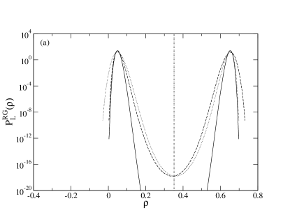
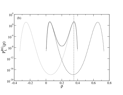
Figure 4: (a). The solid curve shows the form of $P^{RG}_{L}(\rho)$ for the case $\rho_{0}=\rho_{d}$, for which $\rho_{-}=\rho_{g}$ and $\rho_{+}=\rho_{l}$. Also shown (dashed curve) is the underlying GCE coexistence input distribution $P_{L}(\rho)$ and the reflected and shifted distribution $P_{L}(2\rho_{0}-\rho)$ (dotted line) that feature in the transformation Eq. (7). (b). The corresponding data for the case $\rho_{0}=(\rho_{g}+\rho_{d})/2$, for which $\rho_{-}=\rho_{g}$ and $\rho_{+}=\rho_{d}$. In both parts the coexistence diameter is represented by a vertical dot-dashed line.

Eq. (12) implies that if one can determine the coexistence diameter from a RGE simulation, then one can simply read off the coexistence densities from the corresponding peaks in $P^{RG}_{L}(\rho|\rho_{d})$. In practice, one can estimate $\rho_{d}$ by requiring consistency between Eq. (12) and Eq. (13) and/or Eq. (14). The consistency condition is readily implemented graphically as shown in Fig. 5: one simply plots the measured values of $\rho_{\pm}$ versus $\rho_{0}$, together with the transformed points $\rho_{\pm}$ versus $2\rho_{0}-\rho_{\pm}$. The two sets of data intersect at $\rho_{0}=\rho_{d}$ and the coexistence densities can be read off from the position of the RGE peaks at this value of $\rho_{0}$ . The implementation of this “intersection method” is shown in Fig. 5.

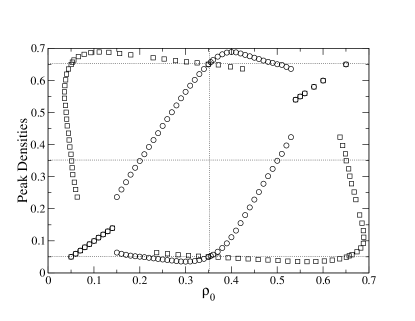
Figure 5: Illustration of the intersection method. Circles show the RGE peak densities $\rho_{-}$ and $\rho_{+}$ of Fig. 3 as a function of $\rho_{0}$. Also shown are the transformed points, $2\rho_{0}-\rho_{\pm}$, (squares). The two data sets intersect at the diameter (vertical dot-dashed line).

In order to gauge the accuracy of our intersection method, we tabulate in Tab. 2 the results of applying it at a number of subcritical temperatures spanning the range $0.7\lesssim T/T_{c}\lesssim 0.94$. Clearly there is excellent agreement between the coexistence densities obtained from the intersection method and those obtained directly from the underlying GCE coexistence density distribution. Such discrepancies as are evident are largest at temperatures close to criticality where the positions of peaks in a density distribution anyway serve as a poor measure of coexistence densities due to finite-size effects wilding1995a .

	GCE			RGE
$T/T_{c}$	$\rho_{d}$	$\rho_{g}$	$\rho_{l}$	$\rho_{d}$	$\rho_{g}$	$\rho_{l}$
0.937	0.3320(16)	0.1095(12)	0.554(4)	0.3352(14)	0.1096(8)	0.5608(22)
0.865	0.3473(24)	0.0607(8)	0.6342(44)	0.3482(20)	0.0600(10)	0.6363(44)
0.844	0.3517(22)	0.05079(74)	0.6526(44)	0.3513(24)	0.04998(66)	0.6527(42)
0.833	0.3538(26)	0.0467(8)	0.6611(50)	0.3537(22)	0.04598(50)	0.6615(42)
0.813	0.3582(12)	0.0396(12)	0.6769(26)	0.3583(16)	0.0390(4)	0.6777(32)
0.796	0.3619(30)	0.0342(2)	0.6896(60)	0.3616(26)	0.03378(30)	0.6895(54)
0.695	0.3847(12)	0.01360(8)	0.756(2)	0.3854(14)	0.013698(90)	0.7572(26)

Table 2: Estimates of the coexistence densities $\rho_{g}$ and $\rho_{l}$, together with the coexistence diameter $\rho_{d}$ for the 3D LJ fluid described in Sec. III at a selection of sub-critical temperatures. The GCE estimates of $\rho_{g,l}$ derive from the densities of the peaks in the coexistence form of $P_{L}(\rho)$; $\rho_{d}$ follows as their average. The RGE estimates for $\rho_{d}$ derive from $P^{RG}_{L}(\rho)$ via the intersection method described in the text, while $\rho_{g,l}$ follows from the corresponding peak densities in $P^{RG}_{L}(\rho|\rho_{0}=\rho_{d})$. Error bars are conservative and are calculated via a blocking analysis of the underlying GCE data.

Finally in this section, we note that in the regime of system size and temperature for which a minimum occurs between the peaks of $P_{L}(\rho)$ (rather than a flat portion), the rigorous validity of Eqs. (13) and (14) rests upon the coincidence of the coexistence diameter with the density of this minimum, i.e. on the symmetry of $P_{L}(\rho)$. In general we observe very close, but not perfect, agreement between these two densities. However, in practice it seems that any deviation of the two quantities will impact little on the effectiveness of the intersection method. This is because near its minimum, $P_{L}(\rho)$ is generally much more slowly varying than near its peaks. To elaborate, consider the case $\rho_{0}=(\rho_{g}+\rho_{d})/2$ shown in Fig. 4(b). From the figure one sees that the lower density RGE peak is formed by multiplying the peak in $P_{L}(\rho)$ by the minimum in $P_{L}(2\rho_{0}-\rho)$. As the system size increases, the peak becomes sharper, the minimum becomes flatter, and hence any discrepancy between the density of the minimum and that of the coexistence diameter will have increasingly less influence on the location of the low density peak of $P^{RG}_{L}(\rho)$. The same argument holds for the high density peak of $P_{L}^{RG}(\rho)$ at $\rho_{0}=(\rho_{g}+\rho_{d})/2$. Of course, in the limit in which the central range of $P_{L}(\rho)$ becomes flat, the values of $\rho_{-}$ (and $\rho_{+}$) will become independent of $\rho_{0}$ for a range of values of $\rho_{0}\approx\rho_{d}$. Under these circumstances the coexistence densities can simply be read off as the values of these constant densities.

V Near-critical finite-size scaling

V.1 Symmetric fluids

The near-critical finite-size scaling properties of the RGE have been considered in two previous studies. The first by Mon and Binder Mon1992 focused attention on determining the critical temperature for a lattice gas model, the critical density being known a-priori by virtue of particle-hole symmetry. Whilst successful with respect to its aims, this study provided no insight into how to determine the critical parameters for off-lattice fluids. The second study, by Bruce Bruce97 , provided elucidation of the scaling form of the critical point density distribution (and its relationship to the critical Ising magnetisation distribution), but here too no method was given for locating criticality in realistic fluids within the RGE.

Here we build on these studies by providing a simple prescription for locating critical points for off-lattice fluids. To begin with, however, we shall follow Mon and Binder’s lead by seeking inspiration from a model exhibiting particle-hole symmetry –namely the Ising lattice-gas model – and consider the fluctuations in the density $\rho$. We shall first discuss the critical limit before moving on to the near-critical region.

V.1.1 The critical limit

In the critical limit $t\equiv(T-T_{c})/T_{c}\to 0$, $h\equiv(\mu-\mu_{c})/\mu_{c}\to 0$, and for sufficiently large $L$, $P_{L}(\rho)$ adopts the well known universal scaling form Binder1981

$$P_{L}(\rho|\mu_{c},T_{c})=a_{L}p^{\star}(a_{L}(\rho-\rho_{c}))\>.$$ (15)

Here $a_{L}=a_{1}L^{\beta/\nu}$, with $a_{1}$ a non-universal scale factor, while $\beta\approx 0.326$ and $\nu\approx 0.630$ are the usual critical exponents for the order parameter and the correlation length respectively FISHER98 . $p^{\star}$ is a universal scaling function, which is symmetric (even) with respect to the mean density $\rho_{c}$. Its form is characteristic of the Ising universality class, and is well established from previous simulations studies of the Ising model in both $d=2$ and $d=3$ NICOLAIDES88 ; TSYPIN00 .

Let us now consider the RGE density distribution $P^{RG}_{L}(\rho|\rho_{0},T_{c})$, and make the choice $\rho_{0}=\rho_{c}$. Then, from the symmetry of the critical grand canonical density distribution, we have that $P_{L}(\rho|\mu_{c},T_{c})=P_{L}(2\rho_{0}-\rho|\mu_{c},T_{c})$. Utilizing Eqs. (7) and (15) now shows that

$$P^{RG}_{L}(\rho|\rho_{c},T_{c})\cong\left[p^{\star}(a_{L}(\rho-\rho_{c}))\right]^{2},$$ (16)

up to an unspecified normalization factor. Thus the critical point RGE distribution matches the square of the known universal fixed point form of the Ising magnetisation distribution, as also previously pointed out by Bruce Bruce97 .

V.1.2 Deviations from criticality

At the critical temperature $T=T_{c}$, the form of $P^{RG}$ for values of $\rho_{0}$ in the vicinity of $\rho_{c}$ can be related to that for $\rho_{0}=\rho_{c}$ by expanding in powers of a reduced density $\varrho_{0}\equiv\rho_{0}-\rho_{c}$. To facilitate ready comparison of the various members of the resulting spectrum, it is further convenient to work with a version of $P^{RG}(\rho)$ having zero mean (recall that $\rho_{0}$ not only controls the form of this distribution, but also sets its mean). To this end we set $x\equiv\rho-\rho_{c}$ and define a shifted GCE density distribution

$${\cal P}_{L}(x|\mu_{c},T_{c})=P_{L}(x+\rho_{c}|\mu_{c},T_{c})\>,$$ (17)

so that

$$P^{RG}(x|\rho_{0},T_{c})={\cal P}_{L}(x+\varrho_{0}|\mu_{c},T_{c}){\cal P}_{L}(-x+\varrho_{0}|\mu_{c},T_{c})\>.$$ (18)

Expanding in the small parameter $\varrho_{0}$, one then finds quite generally that

$$P^{RG}_{L}(x|\rho_{0},T_{c}) = {\cal P}_{L}(x){\cal P}_{L}(-x)$$

$$+ \varrho_{0}\left[{\cal P}_{L}(x){\cal P}_{L}^{\prime}(-x)+{\cal P}_{L}(-x){\cal P}_{L}^{\prime}(x)\right]$$

$$+ \frac{1}{2}\varrho_{0}^{2}\left[{\cal P}_{L}(x){\cal P}_{L}^{\prime\prime}(-x)+2{\cal P}_{L}^{\prime}(x){\cal P}_{L}^{\prime}(-x)\right.$$

$$+\left.{\cal P}_{L}(-x){\cal P}_{L}^{\prime\prime}(x)\right]$$

$$+ \frac{1}{6}\varrho_{0}^{3}\left[3{\cal P}_{L}^{\prime}(x){\cal P}_{L}^{\prime\prime}(-x)+3{\cal P}_{L}^{\prime}(-x){\cal P}_{L}^{\prime\prime}(x)\right.$$

$$+\left.{\cal P}_{L}(x){\cal P}_{L}^{\prime\prime\prime}(-x)+{\cal P}_{L}^{\prime\prime\prime}(x){\cal P}_{L}(-x)\right]$$

$$+ \frac{1}{24}\varrho_{0}^{4}\left[8{\cal P}_{L}^{\prime\prime}(x){\cal P}_{L}^{\prime\prime}(-x)+\dots\right]+\dots\>,$$

where we have abbreviated ${\cal P}_{L}(x)={\cal P}_{L}(x|\mu_{c},T_{c})$.

For models exhibiting particle-hole symmetry, the terms in the expansion (LABEL:eq:genexpan) that involve odd powers of $\varrho_{0}$ drop out and one has

$$P^{RG}_{L}(x|\rho_{0},T_{c}) = {\cal P}_{L}(x){\cal P}_{L}(-x)$$

$$+ \varrho_{0}^{2}\left[{\cal P}_{L}(x){\cal P}_{L}^{\prime\prime}(x)-({\cal P}_{L}^{\prime}(x))^{2}\right]+{\mathcal{O}}[\varrho_{0}^{4}]\>.$$

Thus in the symmetrical case, the leading $\rho_{0}$ dependence of $P^{RG}_{L}(x)$ comes from the $\rho_{0}^{2}$ term. An analogous expansion of $P^{RG}_{L}(x)$ in terms of the reduced temperature $t$ shows that, by contrast, the leading temperature dependence arises from terms linear in $t$.

Together these findings lead us to propose the following finite-size scaling ansatz for $P^{RG}_{L}(x|\rho_{0},T)$, expressed in terms of the reduced variables $\varrho_{0}$ and $t$:

$$P^{RG}_{L}(x|\varrho_{0},t)=b_{L}{\hat{p}}(b_{L}x,b_{2}tL^{1/\nu},b_{3}\varrho_{0}^{2}L^{2\beta/\nu},b_{4}L^{-\theta/\nu})\>.$$ (21)

Here $b_{L}=b_{1}L^{\beta/\nu}$, while $b_{1},b_{2},b_{3},b_{4}$ are non-universal scale factors. ${\hat{p}}$ is a universal scaling function which is symmetric in $x$ for all values of its other arguments. The final term, with associated exponent $\theta\approx 0.52$ GUIDA98 characterizes the leading symmetrical corrections to scaling and accounts for deviations from the large $L$ scaling limit.

Now, a useful dimensionless quantity that characterizes the shape of a distribution is the fourth order cumulant ratio, a common variant of which is defined as

$$Q\equiv\frac{\langle x^{2}\rangle^{2}}{\langle x^{4}\rangle}\>.$$ (22)

The scaling of the cumulant ratio for $P^{RG}_{L}(x|\varrho_{0},t)$ follows from Eq. (21) as

$$Q_{L}(\rho_{0},t)=q(c_{2}tL^{1/\nu},c_{3}\varrho_{0}^{2}L^{2\beta/\nu},c_{4}L^{-\theta/\nu})\>,$$ (23)

with $q$ a universal function. Accordingly in the vicinity of the critical point the cumulant behaves as

$$Q_{L}(\rho_{0},t) = q^{\star}\left[1+c_{2}^{\prime}tL^{1/\nu}+c_{3}^{\prime}\varrho_{0}^{2}L^{2\beta/\nu}\right.$$ (24)

$$+\left.c_{4}^{\prime}L^{-\theta/\nu}+\mathcal{O}(\varrho_{0}^{4},t^{2})\right]\>,$$

where $q^{\star}\equiv q(0,0,0)$ and $c_{2}^{\prime},c_{3}^{\prime}$ and $c_{4}^{\prime}$ are system-specific constants.

For a given $L$ and a fixed choice of $T$, this implies that the variation of $Q_{L}$ with $\rho_{0}$ is parabolic:

$$Q_{L}(\rho_{0},t=0)=q^{\star}\left[{\rm const}.+c_{3}^{\prime}L^{2\beta/\nu}\varrho_{0}^{2}\right]\>.$$ (25)

This latter result can be checked directly for the case $T=T_{c}$ because the universal critical point form $p^{\star}(a_{L}(\rho-\rho_{c}))$ has been parameterized on the basis of accurate measurements of the magnetisation distribution of the critical $3d$ Ising model TSYPIN00 . Fig. 6(a) shows a selection from the spectrum of transformed distributions $P^{RG}_{L}(x|\varrho_{0},t=0)$ for a wide range of values of $\varrho_{0}$. For small values of $\varrho_{0}$, the behaviour of $Q_{L}(\varrho_{0})$ is well described by a parabolic form with $q^{\star}=0.711901$, as confirmed by the fit shown in Fig. 6(b).

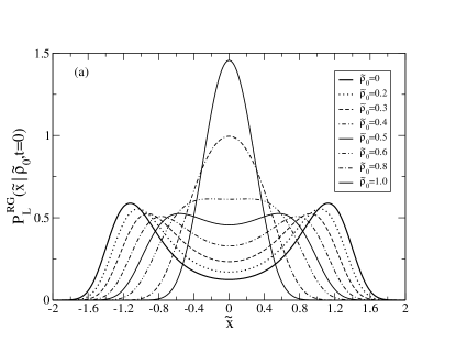
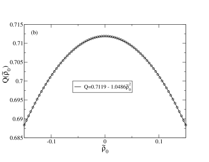
Figure 6: (a) Selections from the universal spectrum of transformed distributions generated at $T=T_{c}$ via Eqs. (15-18) using the estimate for $p^{\star}(\tilde{x})$ parameterized in ref. TSYPIN00 . All distributions are normalised. The scaling variable is $\tilde{x}=b_{1}L^{\beta/\nu}x$, with the non-universal constant $b_{1}$ chosen so that for distribution for $\varrho_{0}=0$ has unit variance. (b) The corresponding behaviour of the cumulant $Q(\tilde{\varrho_{0}})$ together with a parabolic fit. The scaling variable here and in the legend of (a) is $\tilde{\varrho}_{0}=\sqrt{c_{3}}L^{\beta/\nu}\varrho_{0}$.

Finally in this section, it will prove useful to define a special locus in $(\varrho_{0},t)$ space, namely that for which $Q_{L}$ matches $q^{\star}$, which we dub the “iso-$q^{\star}$” line. Let us initially disregard corrections to scaling (i.e. set $c_{4}^{\prime}=0$). Then for points on this line sufficiently close to criticality, it follows immediately from Eq. (24) that

$$\varrho_{0}^{2}=-(c_{2}^{\prime}/c_{3}^{\prime})L^{(1-2\beta)/\nu}t\>,$$ (26)

which is a parabola in the space of $\rho_{0}-T$ whose maximum coincides with the critical point. Now, the presence of corrections to scaling means that at the critical point ($t=\varrho_{0}=0$), $Q_{L}$ will differ from its limiting value $q^{\star}$ by an amount $c_{4}^{\prime}L^{-\theta/\nu}$. Effectively, therefore, in following the iso-$q^{\star}$ parabola to its maximum for a finite-sized system, we miss the critical point by a small deviation. Empirically, one finds that $c_{2}^{\prime}$ and $c_{3}^{\prime}$ are negative [cf. the effect of finite $\varrho_{0}$ in Fig. 6(a)]. Since for Ising-like systems one finds that $c_{4}^{\prime}$ is negative, i.e. corrections to scaling decrease $Q_{L}$ below $q^{\star}$ at criticality NICOLAIDES88 ; wilding1995a , it falls to negative values of $t$ to raise $Q_{L}$ back up to $q^{\star}$. This implies that the maximum of the iso-$q^{\star}$ line occurs at a temperature $T_{c}(L)$ which differs from the true critical temperature according to:

$$T_{c}-T_{c}(L)\propto L^{-(\theta+1)/\nu}$$ (27)

Values of $T_{c}(L)$ obtained from the maximum of the iso-$q^{\star}$ parabola for a number of system sizes can thus be extrapolated to yield an estimate of $T_{c}$.

V.2 Asymmetric fluids

In realistic fluids, the critical point density distribution in the GCE is genuinely symmetric only in the limit $L\to\infty$. For finite-sized systems at criticality, corrections are expected from the fact that the Ising-like scaling fields are not identical to $t$ and $h$, but are instead given by linear combinations of these two variables (“field mixing”) and also the pressure (“pressure mixing”), with in addition quadratic and higher-order corrections in the same variables. The magnitude of these corrections (relative to that of the limiting form $p^{\star}$) decays with $L$ bruce1992 ; wilding1992 ; KIMFISHER04 .

Explicitly, one can confirm by a detailed finite-size analysis Sollich_maybe_2010 the form conjectured by KIMFISHER04 , as an expansion in inverse powers of $L$ and up to quadratic order in $t$:

$$a_{L}^{-1} \!\!\!\!\!\!\!\!P_{L}(\rho|\mu_{c},T)\ =\ p^{*}+jL^{-\beta/\nu}s_{\rm pm}+a_{4}L^{-\theta/\nu}r_{\rm cs}$$

$${}+lL^{(1-\alpha-\beta)/\nu}s_{\rm fm}+a_{2}L^{1/\nu}t\,r_{t}$$

$${}-kL^{(2-\alpha-\beta)/\nu}t\,s_{t,\rm fm}+k^{2}L^{2(2-\alpha-\beta)/\nu}t^{2}\,r_{t^{2},\rm fm}$$

Here $p^{*}$, $r_{\rm cs}$, $r_{t}$, $r_{t^{2},\rm fm}$ are even functions, while $s_{\rm pm}$, $s_{\rm fm}$ and $s_{t,\rm fm}$ are odd; all are evaluated at the scaled density $a_{L}(\rho-\rho_{c})$. All terms on the r.h.s. except for $p^{*}$ have non-universal prefactors which we have written as $j$, $k$, $l$, $a_{2}$ and $a_{4}$. The subscripts indicate where the various contributions come from, according to pm: pressure mixing, cs: corrections to scaling, fm: field mixing, $t$: temperature shift, $t^{2}$: second order in temperature shift.

From $P_{L}(\rho|\mu_{c},T)$ as given above one can find $P_{L}^{RG}(x|\rho_{0},T)$, and then take moments of $x$ to obtain the cumulant ratio $Q$. This basically inherits the structure of the terms in $P_{L}(\rho|\mu_{c},T)$, except for the fact that the asymmetry of $s_{\rm pm}$ and $s_{\rm fm}$ cancels linear contributions in the mixing coefficients:

$$Q_{L}(\rho_{0},t) = q^{*}[1+c_{2}^{\prime}tL^{1/\nu}+c_{3}^{\prime}\varrho_{0}^{2}L^{2\beta/\nu}+c_{4}^{\prime}L^{-\theta/\nu}\ \ \ \ \ {}$$

$${}+\ldots j^{2}L^{-2\beta/\nu}+\ldots jkL^{(2-\alpha-2\beta)/\nu}t$$

$${}+\ldots k^{2}L^{2(2-\alpha-\beta)/\nu}t^{2}$$

$${}+\ldots j\varrho_{0}L^{-2\beta/\nu}+\ldots k\varrho_{0}L^{(2-\alpha-2\beta)/\nu}]$$

The dots ($\ldots$) indicate factors of order unity that are determined by the various universal functions $r$ and $s$. It is then easy to see, by setting $\partial Q_{L}/\partial\varrho_{0}=0$, that the extremum of any line of constant $Q_{L}$ in the $(\varrho_{0},t)$ plane occurs at

$$\varrho_{0}=\ldots jL^{-2\beta/\nu}+\ldots kL^{(2-\alpha-2\beta)/\nu}t$$ (30)

rather than at $\varrho_{0}=0$ as in our previous analysis without field and pressure mixing. Inserting back into (V.2) then shows that the value of $Q_{L}$ on any iso-$Q_{L}$ line has, as a function of the reduced temperature $t$ at the maximum, the same form as the r.h.s. of (V.2) but with the $\varrho_{0}$-dependent terms omitted and the dots now representing different prefactors of order unity. By setting $Q_{L}=q^{*}$ one concludes that the maximum of the iso-$q^{*}$ curve, in particular, lies at the reduced temperature obeying

$$0 = c_{2}^{\prime}tL^{1/\nu}+c_{4}^{\prime}L^{-\theta/\nu}+\ldots j^{2}L^{-2\beta/\nu}$$

$${}+\ldots jkL^{(2-\alpha-2\beta)/\nu}t+\ldots k^{2}L^{2(2-\alpha-\beta)/\nu}t^{2}$$

The corresponding value of $\varrho_{0}$ at the maximum follows by inserting the solution for $t$ into (30).

We have kept track of pressure mixing effects via the coefficient $j$ above, but in non-ionic fluids these are generally weak, i.e. $j$ is very small KIMFISHER04 . To see how mixing effects enter, let us then only keep $k$ for now. If $k$ is small, the condition (V.2) will give the leading scaling $t\sim L^{-(\theta+1)/\nu}$ as before. The last term in (V.2) is then of order $k^{2}L^{2(1-\alpha-\beta-\theta)/\nu}$ and becomes comparable to the first two terms $\sim L^{-\theta/\nu}$ when

$$L\sim k^{-\nu/(1-\alpha-\beta-\theta/2)}$$ (32)

The exponent on the r.h.s. is around -2.07, so if $k$ is small enough then this crossover lengthscale above which field mixing becomes relevant may be too large for us to access. Our numerical results below suggest that this is the case for the specific system studied here.

In Eq. (30), the pressure mixing term is generally subleading because of its $L$-dependence, so that $\varrho_{0}\sim kL^{(2-\alpha-2\beta)/\nu}t$. Even if mixing is too weak to be observed in the $L$-dependence of $t$, it will therefore be evident in an $L$-dependence of $\varrho_{0}$. In the specific case where $t\sim L^{-(\theta+1)/\nu}$, this dependence would be

$$\varrho_{0}\sim kL^{(1-\alpha-2\beta-\theta)/\nu}$$ (33)

with exponent $\approx-0.45$.

V.3 Computational method

Following the iso-$q^{\star}$ parabola to its maximum provides a convenient route to the effective critical parameters. In practice, this is achieved via the following computational prescription.

1. For a given system size $L$, perform a RGE simulation for some value of $\rho_{0}$ and $T$ to obtain $P^{RG}_{L}(\rho|\rho_{0},T)$.

2. Deploy histogram reweighting ferrenberg1989 to locate the temperature for which $Q_{L}(T|\rho_{0})=q^{\star}=0.711901$.

3. Repeat for a range of $\rho_{0}$ values to yield the iso-$q^{\star}$ curve in $\rho_{0}-T$ space.

4. A parabolic fit to the estimates for the iso-$q^{\star}$ curve will pinpoint its maximum or – should it prove necessary – guide the choice of parameters for further simulations nearer to criticality.

5. The coordinates of the maximum of the iso-$q^{\star}$ parabola serve as estimates for $\rho_{c}(L)$ and $T_{c}(L)$. Results from a range of system sizes can be extrapolated to the thermodynamic limit according to Eqns. (33) and (27).

With regard to this procedure, we make the following observations. Firstly, our approach explicitly assumes that the universality class and the associated value of $q^{\star}$ are known a-priori. In most cases of current interest, fluid criticality appears to be Ising-like, and hence the above procedure should provide a precise and efficient procedure for estimating $T_{c}$ and $\rho_{c}$. However, in cases where the universality class is in doubt, or one simply wishes to perform a consistency check on one’s measurements, a procedure can be implemented analogous to that proposed by Kim and Fisher KIMFISHER03 for the GCE density distribution. By scanning $\rho_{0}$ at some prescribed $T$, one can locate the maximum of the parabola $Q(\rho_{0}|T)$ (cf. Eq. (25)). Repeating for a range of $T$ (via histogram reweighting) allows the determination of the line of $Q$ maxima in $\rho_{0}-T$ space. Estimates of $Q$ along this line, and for a range of system sizes, should exhibit “cumulant crossing” Binder1981 at the estimated critical point, and for a value of $Q=q^{\star}$ characteristic of the appropriate universality class. Correspondingly the finite size forms of $P^{RG}_{L}(x)$ should all collapse onto a universal scaling function.

V.4 Results

In order to investigate the finite-size scaling properties of the RGE, we have generated near-critical forms of $P^{RG}_{L}$ from GCE density distributions via the transformation Eq. (7).

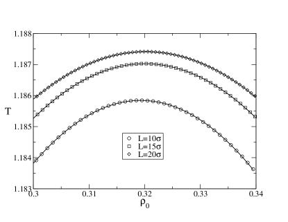
Figure 7: Measured iso-$q^{\star}$ curves for the LJ fluid for system sizes $L=10,\ 15,\ 20$. Uncertainties are considerably smaller than the symbol sizes. Also shown (curves) are parabolic fits; maxima provide estimates of the critical temperature $T_{c}(L)$ and density $\rho_{c}(L)$.

Measurements of the iso-$q^{\star}$ curve for the system sizes $L=10,\ 15,\ 20$ are shown in Fig. 7(a) together with a parabolic fit. Clearly the data are well described by a parabolic form, but the positions of the maxima vary considerably.

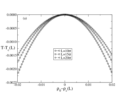
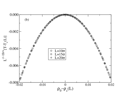
Figure 8: (a) The iso-$q^{\star}$ curves of fig. 7 shifted so that their maxima lie at a common origin. Statistical errors are smaller than the symbol sizes; lines are guides to the eye. (b) The same data plotted in terms of the scaling variable $L^{(1-2\beta)/\nu}t$, with $\beta=0.326,\nu=0.63$.

In order to expose the scaling behaviour of the iso-$q^{\star}$ curves we have shifted the data so that the maxima coincide with the origin, as shown in Fig. 8(a). We then scale the temperature axis by $L^{(1-2\beta)/\nu}t$, as predicted by Eq. (26) to obtain the results shown in Fig. 8(b). This indeed shows an excellent data collapse.

The coordinates of the iso-$q^{\star}$ maxima serve as estimates for the effective critical parameters $T_{c}(L),\rho_{c}(L)$. The finite-size dependence of these estimates are plotted in Figs. 9(a) and (b) respectively in terms of the anticipated scaling variables (cf. Eqs. (27) and (33)). As anticipated above, data for $T_{c}(L)$ are most consistent with the scaling $t\sim L^{-(\theta+1)/\nu}$, suggesting that field mixing effects on this quantity are weak, at least for the system sizes we have studied. An extrapolation of the data for $T_{c}(L)$ (Fig. 9(a)) yields $T_{c}=1.1878(2)$. As regards $\rho_{c}(L)$, the range of accessible system sizes and the rather large error bars unfortunately prevent us from establishing convincingly the predicted $L$-dependence (33). The error bars were determined from a blocking analysis and one notes that those for $T_{c}(L)$ are relatively much smaller than those on $\rho_{c}(L)$. The reason for this are twofold. Firstly the iso-$q^{\star}$ curves have quite small curvature (cf. the scales of  Fig. 7) so that any uncertainty in $T$ translates to a larger uncertainty in $\rho$. A further problem is that for the smaller system sizes the resolution of the density scale $\Delta\rho=1/V$ limits the precision with which the maximum can be determined. For instance for $L=10$, the density resolution is $\Delta\rho=0.001$ which is large on the scale of the finite size shifts we observe overall. If we restrict our extrapolation to a fit based only on the five largest system sizes shown in Fig. 9(b), we find $\rho_{c}=0.3210(3)$. The present estimates for $T_{c}$ and $\rho_{c}$ are to be compared with previous older estimates (based on a more limited range of system sizes) of $T_{c}=1.1876(3),\rho_{c}=0.3197(4)$. wilding1995a .

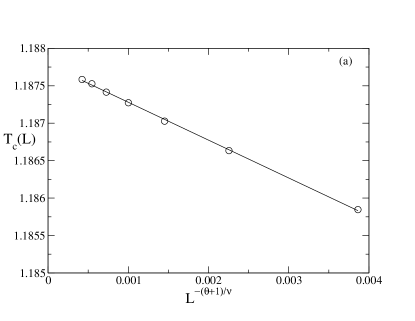
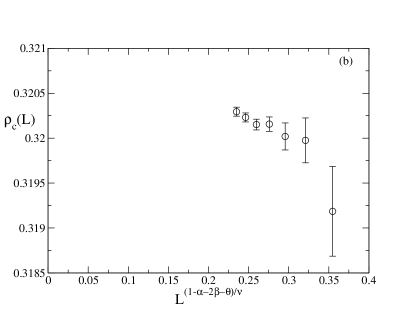
Figure 9: (a) Measured estimates of $T_{c}(L)$ from the maxima of the iso-$q^{\star}$ curve. The data is plotted against the scaling variable $L^{(\theta+1)/\nu}$ and a straight line fit shows the quality of the scaling. Statistical errors do not exceed the symbol sizes. (b) Measured estimates of $\rho_{c}(L)$ from the maxima of the iso-$q^{\star}$ curves, plotted against the anticipated scaling variable, Eq. (33)

VI Summary and conclusions

The aim of the work described in this paper was to lay firm foundations for future investigations of phase behaviour within the Restricted Gibbs ensemble. To this end we have developed new approaches for determining both the coexistence and critical point parameters within this ensemble.

In the subcritical regime, we have proposed and tested an “intersection method” for estimating the coexistence densities. This involves measurements of the RGE peak densities as a function of the overall system density $\rho_{0}$. Comparison of the resulting data with a transformed version of itself yields an intersection at a density that serves as an estimate of the coexistence diameter $\rho_{d}$. The coexistence densities are then simply read off from the RGE peak densities for $\rho_{0}=\rho_{d}$. In tests, the results agreed to high precision with independently determined estimates of the coexistence properties.

In the near-critical region, we have described (and extended) a finite-size scaling method (elements of which were originally outlined in ref. LIU2006 ) for obtaining accurate estimates of fluid critical point parameters within the RGE. The strength of this method is that it provides estimates of effective (finite-size) critical parameters via a simple and convenient parabolic fit to measurements of a cumulant ratio. These estimates can be extrapolated to the thermodynamic limit using appropriate scalings forms which we have presented both for the case of particle-hole asymmetry and for asymmetric fluids. We expect the method to be useful when one has prior knowledge of the universality class and the associated value of $q^{\star}$.

In addition to its utility for extracting critical point parameters from RGE simulations of fluids, we remark that our analysis provides an alternative to traditional routes for obtaining these properties in GCE simulations. Specifically, as we have shown, one can apply the transformation of Eq. (7) to near-critical GCE data and then proceed as if the density distribution had been obtained within the RGE. The subsequent analysis in terms of the scaling of iso-$q^{\star}$ maxima is arguably simpler to implement than a widely used approach for GCE data wilding1995a in which one determines a symmetrized ordering operator distribution via a linear field mixing approximation, and matches this distribution to a universal form to obtain effective critical parameters.

Finally, with regard to the wider context of this work, it should be stressed that RGE simulations cannot be regarded as competitive with the GCE in situations where the latter operates efficiently, e.g. for single component fluids or mixtures of similarly sized particles. Specifically, the lack of a chemical potential field implies that histogram reweighting cannot be implemented to scan a range of overall densities or concentrations on the basis of a single simulation run; instead a separate RGE simulation is required for each density $\rho_{0}$ of interest. Where we expect the RGE to come into its own, is for highly size-asymmetric mixtures, for which GCE sampling becomes ineffectual. As shown in ref. LIU2006 the Generalized Cluster algorithm, when combined with the RGE, does permit efficient sampling of configuration space in such systems, and thus the methods we have described should facilitate the accurate determination of phase coexistence properties. We have already begun applying them in this context and hope to report on our progress in due course.

- (1) J. Liu, N.B. Wilding, and E. Luijten, Phys. Rev. Lett. 97, 115705 (2006).
- (2) J. Liu and E. Luijten, Phys. Rev. Lett. 92, 035504 (2004).
- (3) A.Z. Panagiotopoulos, Mol. Phys. 61, 813 (1987).
- (4) K.K. Mon and K. Binder, J. Chem. Phys. 96, 6989 (1992).
- (5) A.D. Bruce, Phys. Rev. E 55, 2315 (1997).
- (6) N.B. Wilding, Phys. Rev. E 52, 602 (1995).
- (7) D. Frenkel and B. Smit, Understanding Molecular Simulation (Academic, San Diego, 2002).
- (8) C. Borgs and R. Kotecky, Phys. Rev. Lett. 68, 1734 (1992).
- (9) J.R. Errington, Phys. Rev. E 67, 012102 (2003).
- (10) K. Binder, Z. Phys. B 43, 119 (1981).
- (11) M.E. Fisher and S.-Y. Zinn, J. Phys. A 31, L629 (1998).
- (12) D. Nicolaides and A.D. Bruce, J. Phys. A 21, 233 (1988).
- (13) M. M. Tsypin and H. W. J. Blöte, Phys. Rev. E 62, 73 (2000).
- (14) R. Guida and J. Zinn-Justin, J. Phys. A 31, 8103 (1998).
- (15) A.D. Bruce and N.B. Wilding, Phys. Rev. Lett. 68, 193 (1992).
- (16) N.B. Wilding and AD Bruce, J. Phys.: Condens. Matter 4, 3087 (1992).
- (17) Y.C. Kim and M.E. Fisher, J. Phys. Chem. B. 108, 6750 (2004).
- (18) A.M. Ferrenberg and R.H. Swendsen, Phys. Rev. Lett. 63, 1195 (1989).
- (19) P. Sollich (unpublished).
- (20) Y.C. Kim and M.E. Fisher, Phys. Rev. E 68, 041506 (2003).