A Simple-Minded Unitarity Constraint
and an Application to Unparticles.

Abstract

Unitarity, a powerful constraint on new physics, has not always been properly accounted for in the context of hidden sectors. Feng, Rajaraman and Tu have suggested that large (pb to nb) multi-photon or multi-lepton sugnals could be generated at the LHC through the three-point functions of a conformally-invariant hidden sector (an “unparticle” sector.) Because of the conformal invariance, the kinematic distributions are calculable. However, the cross-sections for many such processes grow rapidly with energy, and at some high scale, to preserve unitarity, conformal invariance must break down. Requiring that conformal invariance not be broken, and that no signals be already observed at the Tevatron, we obtain a strong unitarity bound on multi-photon events at the (10 TeV) LHC. For the model of Feng et al., even with extremely conservative assumptions, cross-sections must be below 25 fb, and for operator dimension near 2, well below 1 fb. In more general models, four-photon signals could still reach cross-sections of a few pb, though bounds below 200 fb are more typical. Our methods apply to a wide variety of other processes and settings.

I Introduction

The current era is dominated by hadron colliders, where small signals must be extracted from very large data sets. In order that new physics of an unfamiliar sort not be missed, it is important to consider a wide variety of possible signals that the experimenters might encounter. In this spirit, there has been considerable activity aimed at thinking broadly about reasonable non-minimal extensions of the standard model Higgs sector, of minimal supersymmetric models, and so forth. While there are strong motivations for each of these classes of models, the simplicity of their minimal versions is motivated mainly by aesthetic considersations. Moreover, the extra particles in non-minimal versons can lead to completely different phenomenological signals from those arising in the minimal versions. Given the baroque nature of the standard model, we would be unwise when addressing important issues in particle physics not to consider the possibility of particles and forces beyond the minimal set required.

Considerable attention has been paid recently to hidden sectors that couple to the standard model at or near the TeV scale. These include “hidden valleys” hv1 ; hv2 ; hvsusy , new sectors with mass gaps and non-trivial dynamics, which lead to new light neutral particles, often produced in clusters and with a boost, and possibly with macroscopically long lifetimes. Hidden valleys are especially natural hosts for dark matter, and indeed a class of hidden valley models hvdark are a popular explanation for current anomalies in dark-matter experiments.

Work on hidden sectors also includes a great deal of research on conformally invariant hidden sectors, dubbed “unparticles” in Un1 ; Un2 ; allunparticle (see also RS2 ; HEIDI ). New sectors with conformally-invariant physics (or at least scale-invariant physics, though there are no known examples of theories in four dimensions with scale invariance but without conformal invariance) can produce large missing-tranverse-momentum (“MET”) signals, and can produce smaller, but potentially still dramatic, visible effects. However, the literature on this subject is full of contradictions, and many claims of interesting effects have been criticized. This has left the experimental community without clear guidance as to how to search for hidden sectors of this type.

Our goal in this paper is to bring some clarity, through simple arguments, to a claim FengRajTu that large production rates for multi-particle final states can be generated through the three-point function of hidden sector operators that couple to the standard model. (Other work emphasizing the importance of higher-point functions, often called “unparticle interactions,” can be found in hvun ; GeorgiUnInts . Additional subtle issues are addressed in Un2 ; allunparticle ; unFox ; unDelgado ; Grinstein .) We consider specifically the mechanism discussed by Feng, Rajaraman and Tu in FengRajTu , slightly generalized. In FengRajTu it was pointed out that (for example) if a scalar primary operator ${\cal O}$ in the hidden sector couples to two gluons and also to two photons, and has a non-trivial three-point function $\langle{\cal O}{\cal O}{\cal O}\rangle$, then the process $gg\to\gamma\gamma\gamma\gamma$ can be generated. Because the form of a three-point function $\langle{\cal O}_{1}{\cal O}_{2}{\cal O}_{3}\rangle$ of primary scalar operators is precisely determined in conformal field theory in terms of the dimensions $\Delta_{i}$ of the three operators ${\cal O}_{i}$, the kinematics of any process of this type is precisely known. (This is also true in some cases for three-point functions involving operators with non-zero spin.) In the case considered by FengRajTu , all kinematic distributions can be calculated in terms of the dimension and spin of ${\cal O}$.

Moreover, there is only one unknown parameter, the overall coefficient of the three-point function (equivalently the OPE coefficient connecting ${\cal O}{\cal O}\to{\cal O}$.) In FengRajTu it was pointed out that as of yet there is no known bound in four-dimensions on the size of this coefficient, and so it was suggested it could be arbitrarily large. Based on the limits from Fermilab on multi-photon events, it was claimed in FengRajTu that LHC production rates (at 14 TeV) were little constrained, and could range as large as 4 pb for $\Delta_{\cal O}\sim 1.1$ and 8 nb (ten times larger than the $t\bar{t}$ cross-section) for $\Delta_{\cal O}\sim 1.9$. Given that four-photon backgrounds are tiny, and that the photons produced in this process have very high $p_{T}$, this would be a truly spectacular signal by any measure.

In this paper we throw some amount of cold water on this possibility. We first observe a simple-minded (and model-independent) unitarity constraint on any hidden sector, conformal or not. Then we show how this specifically constrains conformally-invariant sectors, where explicit computations are possible due to the conformal invariance. After putting some experimental and theoretical limits on the size of the coupling between the two sectors, we apply this constraint specifically to the process $pp\to\gamma\gamma\gamma\gamma$. For the specific case studied in FengRajTu , we find the maximum cross-section (for LHC at 10 TeV) is actually of order 20 fb. When we generalize the scenario considered in FengRajTu by allowing the two gluons to couple to one operator ${\cal O}_{1}$ and the two photons to couple a different operator ${\cal O}_{2}$, we find that the maximum cross-section is anywhere from several pb, in the region $\Delta_{1}\sim 1.4$ and $\Delta_{2}\sim 1.1$, down to 30 fb or below for $\Delta_{1}+2\Delta_{2}>5$.

Our methods can be applied more widely to various other processes. They will strongly constrain four-lepton production through vector unparticles, for example, and any other similar process.

As this paper neared completion some additional work on this subject appeared in fourleptons ; new4gamma . We believe that application of our methods would affect the conclusions of these papers. Also, in new4gamma production of multiple particles through exchange of two unparticles was considered. While we do not address this issue in our current paper, there are additional and related unitarity bounds on this process which were not considered in new4gamma . It should also be noted that the authors of new4gamma assumed in their calculation that there is no important four-point function among the hidden-sector operators, which is not universally true.

The paper is organized as follows. We will explain our unitary bound in section II. After some general comments in section III about applications to unparticle sectors, we will show how to apply it to the specific case of $gg\to\gamma\gamma\gamma\gamma$ in section IV. Section V will be devoted to obtaining a bound on the scale $\Lambda_{1}$ characterizing the coupling between the two gluons and the unparticle sector. In section VI we will calculate the numerical bounds on $pp\to\gamma\gamma\gamma\gamma$. We will comment on other possible processes in section VII, and state some conclusions in section VIII.

II A trivial unitarity bound

We begin by pointing out an essentially trivial but rigorous unitarity bound that governs parton-parton cross-sections for hidden-sector production. The point, simply stated, is that no one process that involves the hidden sector can have a rate that exceeds the total rate for all such processes.

This simple-minded and obvious point becomes useful when the total rate can be computed. Among the situations where this is possible is the case when the hidden sector is a conformal field theory to which the standard model (SM) couples via a local interaction. In this case the total cross-section is given by the square of a standard-model amplitude times the imaginary part of a two-point function of a local operator in the conformal field theory (recently given the name “unparticle propagator” Un1 .) Consequently, one may calculate the bound on the sum of all processes involving the hidden sector.

Let us make a technically more precise statement of this unitarity bound. Suppose the interaction between the two sectors is governed by a local interaction, for example of the form

$${1\over\Lambda^{\delta}}\psi_{A}\psi_{B}{\cal O}$$ (1)

where $\psi_{A,B}$ are SM fields that create the SM partons $A,B$, and ${\cal O}$ is a gauge-invariant operator in the hidden sector that carries no SM charges. (We take ${\cal O}$ to be spinless for the moment, but our statements generalize for any spin.)

We consider first a process $AB\to X$ where $X$ is a state in the hidden-sector Hilbert space. We will refer to the sum over all such states as $AB\to\left\{X\right\}$. Then the optical theorem assures that for center-of-mass momentum $q^{\mu}=q_{A}^{\mu}+q_{B}^{\mu}$ and center-of-mass energy $\sqrt{\hat{s}}=q^{2}$,

$$\sigma(AB\to\{X\};\hat{s}) \equiv \sum_{X}\sigma(AB\to X;\hat{s})$$ (2)

(3)

$$= \frac{{\rm Im}(AB\to\{X\}\to AB)}{\hat{s}}=\frac{\left|\langle AB|\psi_{B}\psi_{A}|0\rangle\right|^{2}}{\Lambda^{2\delta}}\frac{{\rm Im}\left[i\langle 0|{\cal O}(q){\cal O}(-q)|0\rangle\right]}{\hat{s}}\ .$$ (4)

(5)

Corrections to this last formula are smaller than the leading expression by a factor of order $(\hat{s}/\Lambda^{2})^{\delta}$. We simplify notation by defining

$$f_{AB}\equiv\langle AB|\psi_{B}\psi_{A}|0\rangle\ \ ;\ \ G_{{\cal O}}(q;\Lambda)\equiv i\langle 0|{\cal O}(q){\cal O}(-q)|0\rangle$$ (6)

so that

$$\sigma(AB\to\{X\};\hat{s})={1\over\Lambda^{2\delta}\hat{s}}|f_{AB}|^{2}{\rm Im}\left[G_{\cal O}(q;\Lambda)\right]$$ (7)

with $\hat{s}=q^{2}$.

We are effectively assuming that the two sectors are weakly coupled to one another, so that the Hilbert space factors into a SM part and a hidden-sector part. This is true in the limit $\Lambda\to\infty$, and the corrections to this assumption should be small as long as momenta are small compared, naively, to $4\pi\Lambda$. Actually, whether the condition involves $4\pi\Lambda$ or a somewhat smaller scale depends, as we will see, on the operator and on $A,B$. Also we have assumed here that any process generated by two separate couplings of the initial state to the hidden sector, such as considered in new4gamma , is subleading compared to the effect of a single such coupling. If this is not the case, self-consistency problems arise, which we will not address here.

Importantly, as emphasized by our notation, the two-point function of ${\cal O}$ that appears here is the complete two-point function, which includes all effects that depend on $\Lambda$ from the interaction (1), along with any other interactions between the SM and hidden sectors. Let us define the two-point function of ${\cal O}$ in the limit $\Lambda\to\infty$ to be

$$G_{\cal O}^{(0)}(q)\equiv\lim_{\Lambda\to\infty}G_{\cal O}(q;\Lambda)$$ (8)

The difference between this function and the full two-point function includes terms such as

$$G_{\cal O}(q;\Lambda)=G_{\cal O}^{(0)}(q)+iG_{\cal O}^{(0)}(q)^{2}\frac{1}{\Lambda^{2\delta}}\int\frac{d^{4}k}{(2\pi)^{4}}<0|\psi_{B}(k)\psi_{A}(q-k)\psi_{B}(-k)\psi_{A}(k-q)|0>+\dots$$ (9)

as shown in Fig. 1. This particular type of correction sums as usual into a geometric series

$$G_{\cal O}(q;\Lambda)=\frac{G_{\cal O}^{(0)}(q)}{1-G_{\cal O}^{(0)}(q)\Sigma(q)-\dots}$$ (10)

where

$$\Sigma(q)={i\over\Lambda^{2\delta}}\int\frac{d^{4}k}{(2\pi)^{4}}<0|\psi_{B}(k)\psi_{A}(q-k)\psi_{B}(-k)\psi_{A}(k-q)|0>+\dots$$ (11)

as in Fig. 1. Other processes that connect the two sectors will also contribute to the full two-point function.

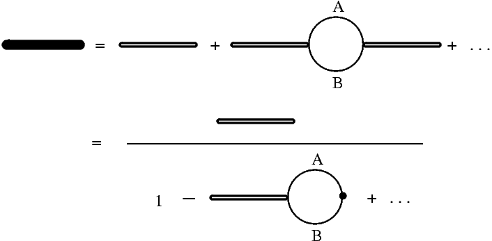
Figure 1: The full two point function for ${\cal O}$ (filled line) differs from the conformal two-point function (unfilled line) by loops of standard model particles; these can be resummed as usual into a geometric series.

Suppose we demand that the full two-point function $G_{\cal O}(q;\Lambda)$ does not differ much from its $\Lambda\to\infty$ limit $G_{\cal O}^{(0)}(q)$ — that is, that the interaction with the SM sector does not strongly alter the hidden sector in the energy regime of interest. (In particular, if the hidden sector is conformal in the $\Lambda\to\infty$ limit, then we are demanding that it remain so to a good approximation.) Then any process such as $AB\to P_{1}P_{2}\dots+X_{0}$, where $P_{i}$ are SM particles and $X_{0}$ is any hidden sector state, and where $P_{i}$ are produced dominantly through SM-hidden sector interactions suppressed by $1/\Lambda$ to some power, can be bounded. In particular, this process will appear in the imaginary part of the full two-point function, suppressed by powers of $1/\Lambda$ to some power. The statement that the $1/\Lambda$ corrections to $G_{\cal O}(q,\Lambda)$ are small, applied to its imaginary part, then implies that

$$\sum_{\{X_{0}\}}\sigma(AB\to P_{1}P_{2}\dots+X_{0}) < {1\over\Lambda^{2\delta}\hat{s}}|f_{AB}|^{2}{\rm Im}\left[G_{\cal O}(q;\Lambda)-G_{\cal O}^{(0)}(q)\right]\$$ (12)

(13)

$$\ll {1\over\Lambda^{2\delta}\hat{s}}|f_{AB}|^{2}{\rm Im}\left[G_{\cal O}(q;\Lambda)\right]\$$ (14)

(15)

$$\approx {1\over\Lambda^{2\delta}\hat{s}}|f_{AB}|^{2}{\rm Im}\left[G_{\cal O}^{(0)}(q)\right]\approx\sigma(AB\to\{X\})$$ (16)

The sum over $X_{0}$ is over any subset of (and including possibly all) allowed hidden-sector states. The corrections to the last approximate equality vanish as $\Lambda\to\infty$. Note the expressions in the first line are of higher order in $1/\Lambda$ than those in the last line, since by definition $G_{\cal O}(q;\Lambda)\to G_{\cal O}^{(0)}$ as $\Lambda\to\infty$. Therefore this is obviously true when $\Lambda\gg q$. But for LHC signals we will be interested in the consequences when $q$ and $\Lambda$ are not well separated.

In English, the relations (12) state the following. The first inequality says that the process in question is found in the imaginary part of $G_{\cal O}$ which does not appear in $G_{\cal O}^{(0)}$, since the latter contains only processes involving the hidden sector alone. The second inequality says that the difference between $G_{\cal O}$ and $G_{\cal O}^{(0)}$ cannot be large, if conformal symmetry is valid. The third approximate equality restates that $G_{\cal O}$ and $G_{\cal O}^{(0)}$ must be similar, so we may use either one. The final approximate equality comes from Eq. (7). The last two inequalities become equalities in the limit $\Lambda\to\infty$.

It is crucial that the constraint (12) depends on $q$, or $\sqrt{\hat{s}}$, the partonic collision energy, not directly on the collider energy $\sqrt{s}$. Thus, at a hadron collider, this constraint must be applied at all relevant values of $\sqrt{\hat{s}}$.

III Application to Conformal Hidden Sectors (Unparticles)

III.1 Conformal invariance must break down

If the hidden sector is conformal, then $G_{\cal O}^{(0)}(q)$ is determined, up to a normalization constant. The canonical normalization is taken so that in position space the time-ordered two-point function is $1/(4\pi^{2}x^{2})^{\Delta}$ (up to contact terms at $x=0$); any other normalization factor can be absorbed into $\Lambda$. The Fourier transform to momentum space yields

$$G_{\cal O}^{(0)}(q)=\frac{1}{(4\pi)^{2\Delta-2}}\frac{\Gamma[2-\Delta]}{\Gamma[\Delta]}(-q^{2}-i\epsilon)^{\Delta-2}\ .$$ (17)

Our normalization is the same as that used in Un1 , simplified by the use of Gamma-function identities.

Suppose we want to use conformal invariance to predict something in the hidden sector. Then we must demand that any corrections to the two-point function are small compared to the two-point function itself, which then implies the bound (12). In particular, for any particular process (such as $gg\to\gamma\gamma\gamma\gamma$, as we will consider below) in which only SM particles $P_{i}$ are produced through the hidden sector,

$$\sigma(AB\to\{X\}\to P_{1}P_{2}\dots P_{n})\ll\sigma(AB\to\{X\})$$ (18)

In fact the bound is much stronger than this; the sum of cross-sections for all such processes, producing any standard model particles and hidden-sector states, is smaller than $\sigma(AB\to\{X\})$. If conformal invariance predicts cross-sections that violate this condition, then it is conformal invariance itself that must be violated, and thus it cannot be used to make predictions.

To illustrate the issues, let us consider a Lagrangian with three terms that couple the SM to the hidden sector through couplings to scalar hidden-sector operators, of the form

$$\delta{\cal L}={1\over\Lambda_{1}^{\delta_{1}}}{\cal O}_{1}\psi_{A}\psi_{B}+{1\over\Lambda_{2}^{\delta_{2}}}{\cal O}_{2}\psi_{1}\psi_{2}+{1\over\Lambda_{3}^{\delta_{3}}}{\cal O}_{3}\psi_{3}\psi_{4}$$ (19)

Here $\delta_{1}=\Delta_{1}+{\rm dim}\psi_{A}+{\rm dim}\psi_{B}-4$, and similarly for $\delta_{2},\delta_{3}$. (For the moment we take all three operators ${\cal O}_{i}$ to be distinct; the case where the operators are related will be dealt with later. We also assume $\delta_{i}>0$; we will discuss this assumption later. The standard model fields $\psi_{i}$, which create particles $P_{i}$, may or may not be different from one another; we make no assumptions about them as yet.) Then, purely from dimensional analysis, we have

$$\sigma(AB\to\{X\};\hat{s})=\frac{N_{0}(\Delta_{1})}{\hat{s}}\left(\frac{\sqrt{\hat{s}}}{\Lambda}\right)^{2\delta_{1}}$$ (20)

where $N_{0}$ is a constant calculable from conformal invariance alone and which depends only on $\Delta_{1}$ and on $|f_{AB}|^{2}$. Meanwhile,

$$\sigma(AB\to P_{i};\hat{s})=\frac{|C_{123}|^{2}}{\hat{s}}N_{P_{i}}(\Delta_{1},\Delta_{2},\Delta_{3})\left(\frac{\sqrt{\hat{s}}}{\Lambda_{1}}\right)^{2\delta_{1}}\left(\frac{\sqrt{\hat{s}}}{\Lambda_{2}}\right)^{2\delta_{2}}\left(\frac{\sqrt{\hat{s}}}{\Lambda_{3}}\right)^{2\delta_{3}}$$ (21)

Here, as emphasized by FengRajTu , $N_{P_{i}}$ is a constant which is determined by the dimensions of the operators ${\cal O}_{i}$. We will see we do not need its exact form. The OPE coefficient $C_{123}$ for ${\cal O}_{1}{\cal O}_{2}\to{\cal O}_{3}$ determines the normalization of the $\langle{\cal O}_{1}{\cal O}_{2}{\cal O}_{3}\rangle$ three-point function. Again, its value will not be needed for our discussion.

These expressions are valid up to the scale $\hat{s}$ where conformal predictions break down. A sufficient condition for such a breakdown would be that $\sigma(AB\to P_{i};\hat{s})\sim\sigma(AB\to\{X\};\hat{s})$. If $\delta_{2}+\delta_{3}>0$, as we are assuming at the moment, then $\sigma(AB\to P_{i};\hat{s})$ grows faster with energy than $\sigma(AB\to\{X\};\hat{s})$. Thus there is always a scale $\hat{s}_{max}$ at which the expressions in Eqs. (20) and (21) become equal. At best, conformal invariance can be used to make predictions only up to this scale. At scales of order or larger than $\hat{s}_{max}$ there must be large corrections to the two-point function of ${\cal O}_{1}$. When this happens, we can predict neither $\sigma(AB\to\{X\})$ — which requires the two-point function directly — nor $\sigma(AB\to P_{i})$ — which is predicted using the special form of the three-point function, whose derivation requires that the two-point function of ${\cal O}_{1}$ be its conformal form.

III.2 Motivation for studying $gg\to\gamma\gamma\gamma\gamma$

We must first decide what physical processes to study, which requires us to address some subtle points. The reader only interested in our results can jump to Sec. IV.

We will focus on processes involving gauge bosons only. Our reasoning is the following. The largest effects from hidden sectors would come from low dimension operators. Scalar operators have the lowest possible dimensions, as is well known from unitarity bounds Mack . (See also SeibergNAD ; ISthreeD for other famous and important applications of these unitarity bounds.) We will discuss operators of non-zero spin in Sec. VII. The only standard-model scalar operators of low dimension are of the form (1) $F_{\mu\nu}F^{\mu\nu}$ or $F_{\mu\nu}\tilde{F}^{\mu\nu}$ for one of the standard model field strengths, (2) the Higgs boson bilinear $H^{\dagger}H$, or (3) $fHf^{\prime}$, where $f$ is a SM fermion doublet and $f^{\prime}$ is a SM fermion singlet.

Large couplings of the form $fHf^{\prime}{\cal O}$ break chiral flavor symmetries and are extremely dangerous, especially for the light quarks found in the proton. Without powerful symmetries or fine-tuning, these interactions will generically induce large and excluded flavor-changing neutral currents, through processes such as $f\bar{f}^{\prime}\to f^{\prime}\bar{f}$, $f\to f^{\prime}\gamma$, etc., mediated via effects of the hidden sector. Conversely, suppressing flavor-changing neutral currents by choosing small couplings (i.e., choosing a very large value for $\Lambda$), reduces all cross-sections involving the hidden sector by factors of $s/\Lambda^{2}$ to a positive power. We are skeptical that there exists an elegant model-building strategy that would permit operators to couple to the light quarks with $\Lambda$ of order 1 TeV and $\Delta$ not far above 1 without risking large $K$-$\bar{K}$ mixing. Conversely, as $\Delta$ approaches 2, our bounds come into force. (Couplings of SM fermions to vector unparticles do not break chiral symmetries and are much more reasonable, but we are only considering scalar operators at the moment.) Consequently, it is far more natural that the initial state coupling should be to gluons.

In the final state, fermionic couplings might have a role to play; for example, flavor-changing constraints on couplings to bottom and top quarks and to tau leptons are somewhat weaker, and one could imagine larger couplings of the heavier fermions to a hidden sector. We will discuss the possibility of a such final states in Sec. VII.

Couplings to Higgs bosons are very interesting but are complicated by the relatively large mass of the Higgs and by its expectation value. Examples of these complications are described in unFox ; unDelgado . To avoid these complications in this paper, we assume that the couplings $H^{\dagger}H{\cal O}$ are not large, which in turn implies that the rates for producing Higgs bosons are small. In any case, Higgs bosons produced through a hidden-sector’s three-point functions will lead mostly to multi-jet states, which have large backgrounds.

For these reasons, in order to keep our presentation simple, we will focus on the process $gg\to\gamma\gamma\gamma\gamma$. This case is nice both because it is conceptually straightforward, is a spectacular LHC signal, and was studied in some detail in FengRajTu . There are nevertheless some fine-tuning issues with the signal, which we discuss below.

III.3 A comment on the naturalness and fine-tuning

On general grounds, when a theory has a low-dimension scalar operator ${\cal O}$, fine-tuning is typically (but not automatically) necessary to avoid generating the operator ${\cal O}$ itself in the Lagrangian. This operator would then itself serve as a relevant perturbation of the conformal field theory and conformal invariance would be lost at very high scales.

To avoid this, one would ask that any such operator transform under a global symmetry, so that its appearance in the Lagrangian is forbidden. For example, ${\cal O}$ might be a pseudoscalar instead of a scalar, or it might transform with a minus sign under some other ${\bf Z}_{2}$ transformation, or be part of a large multiplet under a continuous global symmetry, etc. However, these solutions are not entirely satisfactory since we must in general break this very symmetry to allow terms of the form (19). We might require that the standard model operator also transform under the global symmetry (for example if the ${\cal O}_{i}$ are pseudoscalars we can couple them to $F_{\mu\nu}\tilde{F}^{\mu\nu}$, instead of $F_{\mu\nu}F^{\mu\nu}$ as was done in FengRajTu .) But this is not entirely satisfactory, because a three-point function among three scalar operators transforming under a ${\bf Z}_{2}$ symmetry must vanish, and more complicated symmetries which allow a three-point function cannot generally be realized among SM operators. For example, we cannot couple two gluons to an operator transforming under a ${\bf Z}_{3}$ symmetry without breaking that symmetry.

We might also appeal to supersymmetry to prevent ${\cal O}$ from being generated with a large coefficient. In models where supersymmetry breaking in the hidden sector occurs at a scale which is low compared to the TeV scale, as can occur in models of gauge mediation where the hidden sector learns of supersymmetry breaking only through its coupling to the SM, supersymmetry can forbid the appearance of chiral operators in the superpotential, and thus restrict the operators that appear in the Lagrangian, down to a rather low scale. In this case conformal invariance would still be valid in the regime of interest. But this is not automatic and at the very least involves non-trivial model-building; see for example unNelson .

Even if we solve the problem of generating ${\cal O}$ in the action, there is still the operator ${\cal O}^{\dagger}{\cal O}$, which is usually a relevant operator for $\Delta$ significantly less than $2$. (Note this operator as written may not itself be an operator of definite dimension, but it can be written as a linear combination of such operators, and one of them will generally have dimension less than 4.) The question of whether ${\cal O}^{\dagger}{\cal O}$ is relevant, and, if so, why it is not present with a large coefficient, is analogous to the question of the small value of the Higgs boson mass. In order even to have a discussion about scalar operators with $\Delta$ well below 2, we must assume either that this coefficient is somehow unnaturally suppressed, or that it is protected by a very weakly broken supersymmetry in the hidden sector, as in unNelson . (For interesting but not yet sufficiently powerful results regarding ${\cal O}^{\dagger}{\cal O}$, especially where ${\cal O}$ has dimension less than 2, see RR .)

This particular problem does not arise for $\Delta>2$, where the square of the operator is generally irrelevant. (It has sometimes been erroneously suggested in the literature that scalar “unparticles” do not make sense for $\Delta\geq 2$. But this is simply a misinterpretation of standard singularities which require standard operator renormalization. All conformal field theories contain such operators — for example, the square of the stress tensor.) Our results can be applied to such operators, but as we will see, the bounds that we obtain for such operators are on the verge of putting the signals out of reach of the LHC.

One may also ask about the coupling $H^{\dagger}H{\cal O}$, where $H$ is the standard model Higgs boson. When the Higgs gets an expectation value, this inevitably would generate a breaking of conformal invariance unFox ; unDelgado . Again, if the conformal theory has an exact or weakly broken global symmetry that acts on ${\cal O}$, this operator would be forbidden. (Meanwhile the operator $H^{\dagger}H{\cal O}^{\dagger}{\cal O}$ is generally irrelevant.) In the models we consider below, any such symmetry is broken by the couplings to the standard model. But as long as the high-energy physics that generates these couplings does not directly couple the Higgs boson to the hidden sector, and a symmetry forbids $H^{\dagger}H{\cal O}$ from arising well above the TeV scale, then any $H^{\dagger}H{\cal O}$ term will be suppressed by an extra SM loop factor compared to the leading couplings between the two sectors, and will be sufficiently small not to undermine our assumptions.

Thus to obtain $gg\to\gamma\gamma\gamma\gamma$ from a conformally invariant sector requires quite a bit of work. But we will finesse all these issues, without further comment, in this paper. This is in order to address the specific phenomenological claims of FengRajTu , which assume implicitly that all these issue are resolved, but do not depend on the precise resolution. Also, although they are most easily explained in the case of scalar operators, our methods apply for any spin. At the end of this paper will briefly discuss more realistic settings, such as a three point function involving a vector operator ${\cal V_{\mu}}$, a scalar operator ${\cal O}$, and its conjugate ${\cal O}^{\dagger}$. In this case the operator ${\cal O}$ could be a pseudoscalar, for instance, or carry some additional quantum numbers, and many of these problems would not arise. We emphasize, therefore, that our results are very general and would apply with similar impact in many situations where there are no fine-tuning issues.

III.4 A comment on the far infrared

In general, conformal invariance in the hidden sector may not hold down to arbitrarily low energy. Indeed, we have just discussed various ways in which conformal invariance may be violated at low scales. Moreover, with the couplings that we consider, a truly conformal sector with very light particles can potentially induce new processes that have not been observed, or affect big-bang nucleosynthesis or other aspects of cosmology or astrophysics. For these reasons it may be that the hidden sector has a mass gap at some scale $\mu$, which truncates all the branch cuts in Green functions of hidden-sector operators. (Examples of how this could occur appear in unFox ; unDelgado ; hvun .) We will assume that any such $\mu$ is low enough that (1) it does not impact hidden-sector Green functions above a few tens of GeV, and (2) it does not cause any “hidden valley” signatures, where production of conformal excitations at high energy turns into hidden particles at the scale $\mu$, which in turn decay to standard model particles on detector time scales, giving visible signatures hvun and completely changing the LHC phenomenology. We assume throughout this paper that any infrared effects do not affect the basic unparticle paradigm: that the hidden sector dynamics, for all observable purposes at the Tevatron and LHC, is conformally invariant and therefore predominantly invisible.

IV The bound applied to four-photon events

We now assume that the Lagrangian has couplings between the two sectors of the form

$${\cal L}={1\over\Lambda_{1}^{\Delta_{1}}}{\cal O}_{1}\sum_{a}G^{a}_{\mu\nu}G^{a{\mu\nu}}+{1\over\Lambda_{2}^{\Delta_{2}}}{\cal O}_{2}F_{\mu\nu}F^{{\mu\nu}}$$ (22)

where $G^{a}$ ($a=1,\dots,8$) and $F$ are $SU(3)$ and $U(1)$-electromagnetic field-strength tensors. For consistency, since the events we will study have energies far above the 100 GeV scale, we actually must couple the operator ${\cal O}_{2}$ to hypercharge bosons, with a coefficient $(\Lambda_{2}^{\Delta_{2}}\cos^{2}\theta_{W})^{-1}$. But for brevity we will ignore the associated $\gamma Z$ and $ZZ$ couplings for this paper. Although they contribute comparable three-photon and/or large MET signals, including them would not change the bounds that we obtain, which are in fact bounds on the sum of the cross-sections for all these processes. Thus this omission is conservative, and simplifies our presentation.

Note that we make explicit that ${\cal O}_{1}$ and ${\cal O}_{2}$ are distinct operators, potentially with $\Delta_{1}\neq\Delta_{2}$ and $\Lambda_{1}\neq\Lambda_{2}$. This need not be the case. They might be distinct operators with $\Delta_{1}=\Delta_{2}$, or with equal $\Lambda_{i}$. Or we might take ${\cal O}_{1}={\cal O}_{2}$, as was assumed in FengRajTu ; in this case we could assume $\Lambda_{1}=\Lambda_{2}$, as in FengRajTu , but we need not do so. In this sense our analysis is more general than that of FengRajTu . Indeed we will see the case they considered is much more strongly constrained than is the general situation.

Now let us carry out our argument. Suppose, as we will obtain in the next section, that we have a lower bound on the scale $\Lambda_{1}$ for given $\Delta_{1}$. This is then an upper bound on the cross-section $\sigma(gg\to\{X\};\hat{s})$ for producing anything in the hidden sector via the operator ${\cal O}_{1}$. We could obtain from this a bound on the total hadronic cross-section $\sigma(pp\to\{X\})$ by convolving this bound with the gluon distribution function in the proton. But this is not our goal.

Instead, we turn to any particular process such as $gg\to\gamma\gamma\gamma\gamma$, and require that it not be so large as to make preservation of conformal invariance impossible. In short, we require

$$\sigma(gg\to\gamma\gamma\gamma\gamma;\hat{s})<\sigma(gg\to\{X\};\hat{s})\ \ \ \ (\hat{s}<\hat{s}_{max})$$ (23)

But what $\sqrt{\hat{s}_{max}}$ should we choose?

To choose $\sqrt{\hat{s}_{max}}$ to be the collider energy would be too strong a condition. Most $gg\to\gamma\gamma\gamma\gamma$ events at any collider will occur at energies far below the total collider energy, and so $\sqrt{\hat{s}_{max}}$ need not be nearly so high. To determine the appropriate energy, we must compute the four-photon cross-section as a function of $\hat{s}$, under the assumption of conformal invariance, and see where it is large. Then we should choose $\hat{s}_{max}$ so that the great majority of the $\gamma\gamma\gamma\gamma$ events will be produced at energies below this value.

For example, we might reasonably demand that a certain fraction $\zeta$ of the $gg\to\gamma\gamma\gamma\gamma$ cross-section must occur below the scale $\sqrt{\hat{s}_{max}}$. That is, we define $\hat{s}_{max}$ by

$$\int_{0}^{\hat{s}_{max}}d\hat{s}\ \frac{d\sigma(gg\to\gamma\gamma\gamma\gamma)}{d\hat{s}}=\zeta\int_{0}^{s}d\hat{s}\ \frac{d\sigma(gg\to\gamma\gamma\gamma\gamma)}{d\hat{s}}$$ (24)

where $s$ is the square of the collider center-of-mass energy. To require $\zeta=1$, and therefore $\hat{s}_{max}=s$, would be far too strong, as noted above. If we instead took $\zeta=\frac{1}{2}$ then we would effectively be demanding, typically, that the peak cross-section for $gg\to\gamma\gamma\gamma\gamma$ occurs at $\hat{s}_{max}$, right where conformal invariance is breaking down. In this case, none of the predictions (cross-section or kinematic distributions) of FengRajTu would be at all reliable. For this reason we view $\zeta=\frac{1}{2}$ as unreasonable. We therefore take $\zeta=\frac{2}{3}$ as a conservative choice. This should ensure that the prediction for the rate and differential distributions for $gg\to\gamma\gamma\gamma\gamma$ are given to a rough approximation by conformally invariant calculations, and are not beset with model-dependent effects beyond roughly the 30%–50% level.

Importantly, assuming only that conformal invariance has not been violated, we can determine $\hat{s}_{max}$ in a completely model-independent way that depends only on $\Delta_{1}$ and $\Delta_{2}$. From Eq. (21) (with $\Delta_{1}=\delta_{1}$ and $\Delta_{3}=\Delta_{2}=\delta_{2}$ in the case at hand), we know the precise $\hat{s}$ dependence of the cross-section, up to constants that factor out of the condition in Eq. (24). Defining the $gg$ luminosity function as usual by

$$\frac{dL_{gg}(\tau)}{d\tau}=\int dyf_{g}(\sqrt{\tau}e^{y})f_{g}(\sqrt{\tau}e^{-y})$$ (25)

(where $\tau=\hat{s}/s$) and substituting from Eq. (21), we have, for $\zeta=\frac{2}{3}$,

$$\int_{0}^{\hat{s}_{max}/s}d\tau\frac{dL_{gg}(\tau)}{d\tau}{\tau^{\Delta_{1}+2\Delta_{2}-1}}=\frac{2}{3}\int_{0}^{1}{d\tau}\ \frac{dL_{gg}(\tau)}{d\tau}{\tau^{\Delta_{1}+2\Delta_{2}-1}}$$ (26)

Notice that all dependence on $C_{122}$, $N_{\gamma\gamma\gamma\gamma}(\Delta_{1},\Delta_{2})$ and $\Lambda_{i}$ factors out of this expression. Thus our choice of $\hat{s}_{max}$, once we have chosen a fixed $\zeta$, depends only on $\Delta_{1}+2\Delta_{2}$, and largely scales with $s$ (up to the slow variation of $L_{gg}$ through the evolution of the gluon distribution function.) Table 1 shows $\sqrt{\hat{s}_{max}}$ for a 10 TeV LHC and various choices of $\Delta_{1}+2\Delta_{2}$.

At this point we should mention that throughout this paper our numbers are produced using the (outdated) CTEQ5M pdfs CTEQ5 . This is purely for technical reasons of calculational speed. Results obtained from more modern pdfs differ by significantly less than other systematic errors in our calculations. We have explicitly checked in several cases that our numbers do not change significantly with the MSTW08 pdf set MSTW8 . The errors on $\hat{s}_{max}$ from uncertainties in the gluon pdfs and the appropriate choice of factorization scale are estimated at approximately 5 percent. This is smaller than the dominant source of uncertainty, which arises from the choice of $\zeta$ that defines $s_{max}$. We will have more to say about this uncertainty after we present our results.

$\Delta_{1}+2\Delta_{2}$	3.0	3.5	4.0	4.5	5.0	5.5	6.0
$\sqrt{\hat{s}_{max}}$ (in TeV)	1.2	1.7	2.2	2.7	3.1	3.4	3.7

Table 1: Values of $\sqrt{\hat{s}_{max}}$, at a 10 TeV LHC, for various choices of $\Delta_{1}+2\Delta_{2}$.

Now let us return to the process of obtaining a bound. The bound arises from the fact that $\sigma(gg\to\{X\};\hat{s})$ is precisely known, except for an overall constant normalization, which depends only on $\Lambda_{1}$ and is proportional to $1/\Lambda_{1}^{2\Delta_{1}}$. If $\Lambda_{1}$ is bounded from below, $\Lambda_{1}>\Lambda_{1}^{min}$, then $\sigma(gg\to\{X\};\hat{s})$ is likewise bounded from above, at all $\hat{s}$, by $\sigma(gg\to\{X\};\hat{s};\Lambda_{1}^{min})$.

To understand what this means intuitively, we have plotted $\sigma(gg\to\gamma\gamma\gamma\gamma;\hat{s};\Lambda_{1}^{min})$ and $\sigma(gg\to\{X\};\hat{s})$ in figures 2 to 5, for several different choices of $\Delta_{1}$ and $\Delta_{2}$. The total hidden-sector cross-section $\sigma(gg\to\gamma\gamma\gamma\gamma;\hat{s};\Lambda_{1}^{min})$ is normalized to saturate the bound on $\Lambda_{1}$ that we will obtain later; however for the moment the shape matters more than the normalization. The normalization of the $\gamma\gamma\gamma\gamma$ cross-section $\sigma(gg\to\{X\};\hat{s})$ is chosen so that it does not exceed the total hidden-sector cross-section at any $\sqrt{\hat{s}}$ below $\sqrt{\hat{s}_{max}}$, whose value is indicated by a vertical line. Because of the rate with which the $gg$ luminosity decreases, $\sigma(gg\to\gamma\gamma\gamma\gamma;\hat{s})$ initially increases with energy, until the rapid decrease of the $gg$ luminosity at high $\hat{s}$ overwhelms the rising partonic cross-section. Meanwhile, $\sigma(gg\to\{X\};\hat{s})$ decreases rapidly everywhere. Because of this, we can see by eye that $\hat{s}_{max}$ must be taken quite large, typically of order 1–4 TeV. (This confirms that for $gg\to\gamma\gamma\gamma\gamma$ we can neglect any effects from an infrared scale $\mu$ of the sort discussed in Sec. III.4.) Also, we can see by eye that $\sigma(gg\to\gamma\gamma\gamma\gamma;\hat{s})$ is always vastly less than $\sigma(gg\to\{X\};\hat{s})$, because of the shapes of the two curves, until $\hat{s}$ is very close to $\hat{s}_{max}$.

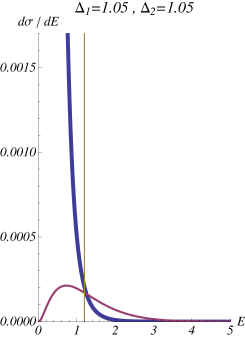
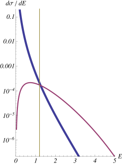
Figure 2: For $\Delta_{1}=1.05,\Delta_{2}=1.05$, the differential cross-sections (in pb/GeV) versus energy $E=\sqrt{\hat{s}}$ (in TeV) for all production processes involving the hidden sector (thick curve) and for four-photon production (thin curve). The right hand plot is the same as the left hand plot, but on a log scale. The total hidden-sector cross-section is normalized by our bound on $\Lambda_{1}$, and the four-photon cross-section is normalized so that it satisfies unitarity, by not exceeding the total for any $\hat{s}<\hat{s}_{max}$. Our estimate of $\sqrt{\hat{s}_{max}}$, determined as explained in the text, is indicated by the vertical line.

As we noted earlier in our more general discussion, dimensional analysis always assures that the ratio $\sigma(gg\to\gamma\gamma\gamma\gamma;\hat{s})/\sigma(gg\to\{X\};\hat{s})$ grows with energy, as long as conformal invariance is applicable. Therefore

$$\frac{\sigma(gg\to\gamma\gamma\gamma\gamma;\hat{s})}{\sigma(gg\to\{X\};\hat{s})}<\frac{\sigma(gg\to\gamma\gamma\gamma\gamma;\hat{s}_{max})}{\sigma(gg\to\{X\};\hat{s}_{max})}<\frac{\sigma(gg\to\gamma\gamma\gamma\gamma;\hat{s}_{max})}{\sigma(gg\to\{X\};\hat{s}_{max};\Lambda_{1}^{min})}\ .$$ (27)

Unitarity requires the last expression be less than one, and writing this condition in terms of the constant coefficients appearing in the formulas (20) and (21) for the cross-sections, we obtain

$$|C_{123}|^{2}N_{\gamma\gamma\gamma\gamma}(\Delta_{1},\Delta_{2})\Lambda_{2}^{-4\Delta_{2}}\ll\left({\hat{s}_{max}}\right)^{-2\Delta_{2}}N_{0}(\Delta_{1})\ .$$ (28)

Notice all $\Lambda_{1}$ dependence factors out of this bound.

Finally we may obtain a bound on the total cross-section for $gg\to\gamma\gamma\gamma\gamma$, namely

$$\sigma(pp\to\gamma\gamma\gamma\gamma) = |C_{123}|^{2}N_{\gamma\gamma\gamma\gamma}(\Delta_{1},\Delta_{2})\Lambda_{1}^{-2\Delta_{1}}\Lambda_{2}^{-4\Delta_{2}}{s^{\Delta_{1}+2\Delta_{2}-1}}\int_{0}^{1}d\tau\frac{dL_{gg}(\tau)}{d\tau}{\tau^{\Delta_{1}+2\Delta_{2}-1}}$$ (29)

$$\ll N_{0}(\Delta_{1})\ \Lambda_{1}^{-2\Delta_{1}}\left({\hat{s}_{max}}\right)^{-2\Delta_{2}}{s^{\Delta_{1}+2\Delta_{2}-1}}\int_{0}^{1}d\tau\ \frac{dL_{gg}(\tau)}{d\tau}{\tau^{\Delta_{1}+2\Delta_{2}-1}}$$

$$< \frac{N_{0}(\Delta_{1})}{s}\ \left(\frac{{s}}{[\Lambda_{1}^{min}]^{2}}\right)^{\Delta_{1}}\left(\frac{s}{\hat{s}_{max}}\right)^{2\Delta_{2}}\int_{0}^{1}d\tau\ \frac{dL_{gg}(\tau)}{d\tau}{\tau^{\Delta_{1}+2\Delta_{2}-1}}$$

This is the formal expression of our main result.

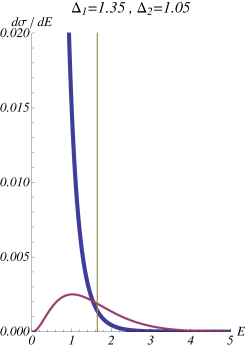
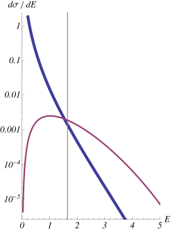
Figure 3: Same as Fig. 2, but with $\Delta_{1}=1.35,\Delta_{2}=1.05$.

Notice that our bound only depends on the collider energy $s$, on the dimensions $\Delta_{1}$ and $\Delta_{2}$, on $\hat{s}_{max}/s$ (determined using Eq. (26) by $\Delta_{1}$ and $\Delta_{2}$,) on $N_{0}$ (which is

$$N_{0}(\Delta_{1})=\frac{-\sin(\pi\Delta_{1})}{(4\pi)^{2\Delta_{1}-2}}\frac{\Gamma[2-\Delta_{1}]}{\Gamma[\Delta_{1}]}\$$ (30)

for a $gg$ initial state,) on the known $gg$ luminosity, and finally on $\Lambda_{1}^{min}$ (which we must separately determine using theoretical and experimental constraints.) All dependence on $\Lambda_{2}$, $N_{\gamma\gamma\gamma\gamma}$ and $C_{122}$ has vanished. If we know $\Lambda_{1}^{min}$ as a function of $\Delta_{1}$ and perhaps $\Delta_{2}$, we can obtain a bound that is model-independent and depends only on $\Delta_{1}$ and $\Delta_{2}$.

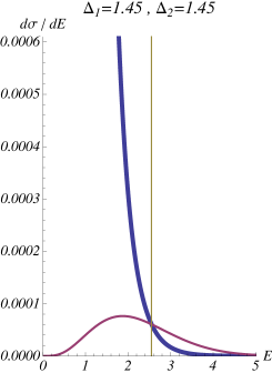
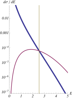
Figure 4: Same as Fig. 2, but with $\Delta_{1}=1.45,\Delta_{2}=1.45$.

V Obtaining bounds on $\Lambda_{1}$

Our only remaining task is to determine $\Lambda_{1}^{min}$. Once we have it, we can compute the bound on the $gg\to\gamma\gamma\gamma\gamma$ cross-section.

We apply two main considerations for constraining $\Lambda_{1}$. The first is that if $\Lambda_{1}$ is too low, then not only is the rate for the invisible process $\sigma(pp\to\{X\})$ very large, the observable process $\sigma(pp\to j+\{X\})$, where $j$ is an initial-state jet, becomes comparable to the standard model rate for jet plus missing transverse momentum (MET). Contraints from Tevatron, mainly from the CDF study CDFjMET , put strong contraints on $\Lambda_{1}$ for low $\Delta_{1}$.

A second constraint on $\Lambda_{1}$ comes from the fact that the coupling of ${\cal O}$ to gluons itself induces corrections to $G_{\cal O}^{(0)}$. We must assume these are small if we are to use conformal invariance to make predictions regarding $gg\to\gamma\gamma\gamma\gamma$. Either such predictions are impossible, invalidating the approach of FengRajTu , or $\Lambda_{1}$ must be larger than some minimum. This puts moderate constraints, of order $1.5$ TeV or larger, which are relevant for larger $\Delta_{1}$ where the experimental constraints are weakest.

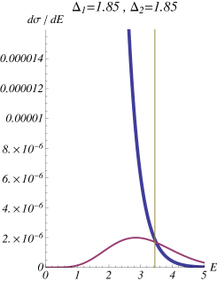
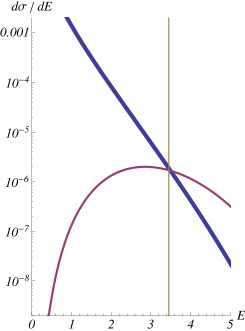
Figure 5: Same as Fig. 2, but with $\Delta_{1}=1.85,\Delta_{2}=1.85$.

V.1 Bounds from Tevatron measurements of monojet events

Given a known partonic cross-section for a hidden-sector process, it is straightforward to compute the rate for jets-plus-MET where the jet(s) only arise from the initial state. One might ask whether emission from the final state could possibly compete with, and perhaps interfere with, this process. The answer regarding interference is “no”; once the hidden state has been produced, it is color neutral, and any final-state radiation must be color singlet, requiring at least two jets be emitted. Similarly, in the model we are considering, the largest interactions between the two sectors involve irrelevant couplings, so any final state radiation process is small at low energy, and is either too small to observe or would show up as a large tail at high energy. Since no such tail is observed at Fermilab, we assume any final-state radiation of jets cannot affect the limits which we will now obtain.

For a conformal hidden sector produced through $gg$, the rate is entirely fixed by $\Lambda_{1}$ and $\Delta_{1}$. For $qg\to q\{X\}$, we find, at leading order,

$$\frac{d\sigma}{dp_{T}^{2}}(qg\to q+\{X\})=C{\sum_{n=0}^{3}}B_{n}\times{{}_{2}F_{1}}\left[\frac{1}{2},-1+\Delta_{1}+n,-\frac{1}{2}+\Delta_{1}+n,\frac{\hat{s}-2\sqrt{\hat{s}}{p_{T}}}{\hat{s}+2\sqrt{\hat{s}}{p_{T}}}\right]\ ,$$ (31)

where $p_{T}$ is the transverse momentum of the jet,

$$C=\frac{4\pi^{2}{\alpha_{s}}}{(2{\pi}{\Lambda})^{2\Delta_{1}}}\frac{\Delta_{1}}{3(3+2\Delta_{1}){\Gamma}[2+2\Delta_{1}]}\frac{({\hat{s}}-2{p_{T}}\sqrt{\hat{s}})^{-1+\Delta_{1}}}{{p_{T}}^{2}{}\sqrt{(1-4{p_{T}}^{2}/{\hat{s}})}}$$ (32)

and

$$B_{0} = \left(-3-2\Delta_{1}+12\Delta_{1}^{2}+8\Delta_{1}^{3}\right)(2-3{p_{T}}^{2}/{\hat{s}})$$ (33)

$$B_{1} = -2(\Delta_{1}-1)\left(3+8\Delta_{1}+4\Delta_{1}^{2}\right)(4-3{p_{T}}^{2}/{\hat{s}})\left(1-\sqrt{4{p_{T}}^{2}/{\hat{s}}}\right)$$ (34)

$$B_{2} = 12(\Delta_{1}-1)\Delta_{1}{}(3+2\Delta_{1})\left(1-\sqrt{4{p_{T}}^{2}/{\hat{s}}}\right)^{2}$$ (35)

$$B_{3} = -8(\Delta_{1}-1)\Delta_{1}{}(\Delta_{1}+1)\left(1-\sqrt{4{p_{T}}^{2}/{\hat{s}}}\right)^{3}$$ (36)

(The reader may compare our result with the literature, see for example Dawson , in the $\Delta_{1}\to 1$ limit.) This is the dominant process at high energy at the Tevatron. There is also the process $gg\to g\{X\}$, but this is smaller in the energy range of interest at the Tevatron and we neglect it. If we included it, our lower bounds on $\Lambda_{1}$ would be stronger.

The CDF experiment CDFjMET has published results on monojet events, in the context of a search for extra dimensions, and a public webpage with additional information and plots is available CDFjMETweb . Early results from DZero D0jMET , with much lower statistics, have not been updated; we will not use them in our analysis. The CDF study uses two sets of cuts, a loose set for a model-independent search, and a tighter set optimized for an extra-dimensions search; we use the former. The data is available in plot form, though not in table form; we have extracted the data directly from the plots, introducing a moderate amount of systematic error in the process. Demanding that the process $qg\to q\{X\}$ not be easily visible above the error bars of the plots in CDFjMET puts a limit on $\Lambda_{1}$ for any given $\Delta_{1}$.

Through this requirement we find limits on $\Lambda_{1}$ shown in boldface in Table 2. There are substantial systematic error bars on our results. First, we have not included the K-factor from loop corrections, or the process $gg\to g\{X\}$; doing so would give a slightly stronger bound. Second, we are not able to include experimental efficiencies and effects of jet energy scale uncertainties; doing so would give a slightly weaker bound. Furthermore, our computation is done at leading order, for which the jet transverse momentum $p_{t}^{jet}$ and the MET are equal. However, both additional jet radiation and jet mismeasurements contribute in the data, so these are not in fact equal, and thus when we extract a limit on $\Lambda_{1}$ it is inherently ambiguous whether we should use the experimental distributions of $d\sigma/d({\rm MET})$ or $d\sigma/d(p_{t}^{jet})$ (and neither is accurate beyond leading order.) Crudely, we estimate that the errors on our determination of $\Lambda_{1}$ are of order 10 percent, which turns out to be a subleading uncertainty compared to that stemming from the ambiguity in choosing $\hat{s}_{max}$.

As final comments, we note that for $p_{t}^{jet}$ of this size, the cross section for $d\sigma/dp_{t}^{jet}$ involves an integral over $q^{2}$ that is insensitive to low $q^{2}$. In other words, our limits on $\Lambda_{1}$ are insensitive to any low-energy cutoff $\mu$. Also, the reader may observe that our calculations do not suffer from the well-known singularity at $\Delta\to 2$ which indicates the need for renormalization. This is because our results depend only on the imaginary part of $G_{\cal O}$. All of our results are smooth as $\Delta$ passes through 2.

V.2 Bounds from preserving conformal invariance

We noted earlier that in a conformal theory perturbed by an interaction of the form Eq. (1), there is an irreducible effect that causes $G_{\cal O}(q;\Lambda)$ to differ from its conformal form $G_{\cal O}^{(0)}(q)$, given by Eq. (10) and shown in Fig. 1.

At leading order, the QCD interactions of gluons play no role, and so we may treat them as a system of free massless particles — a conformal field theory. Thus our calculation is a specific example of a more general issue: if we have two conformal field theories $I$ and $J$, and we couple them through an irrelevant operator ${\cal O}_{I}{\cal O}_{J}$ with coupling $1/\Lambda^{4-\Delta_{I}-\Delta_{J}}$, where ${\cal O}_{I}$ (${\cal O}_{J}$) is a scalar operator in conformal sector $I$ ($J$), then this coupling leads formally to a bad breaking of conformal invariance at some high scale $M_{max}$. More precisely, either conformal invariance is badly broken, or the pointlike coupling ${\cal O}_{I}{\cal O}_{J}$ develops a non-pointlike structure due to new physics at some scale at or below $M_{max}$. Either way, the approximation that one has two conformal field theories coupled by a pointlike operator must break down.

What is an estimate for $M_{max}$? With conventionally normalized operators ${\cal O}_{I}$ and ${\cal O}_{J}$ one might naively guess through naive dimensional analysis that $M_{max}\sim 4\pi\Lambda$. With the normalization used in the unparticle literature (which sets the conventions for our definition of $\Lambda_{i}$ in this paper), this is essentially correct.

However, the standard model operator $\sum_{a}G_{\mu\nu}^{a}G^{a{\mu\nu}}$ is not a conventionally normalized operator of dimension 4, because it contains derivatives. One may easily check that these produce additional factors of $2\pi$ (just as is expected in naive dimensional analysis) leading to a $(2\pi)^{4}$ enhancement relative to the two point function of a conventionally-normalized operator of dimension 4. In addition, there is a factor of $8=3^{2}-1$ from the sum over colors. Altogether this means that, for the normalization of $\Lambda_{1}$ given through the use of the action Eq. (22), which is the same as used by Feng et al. in FengRajTu , the breakdown of conformal invariance occurs well below $4\pi\Lambda_{1}$. This is significant because in the literature one often sees discussion of taking $\Lambda_{1}\sim 1$ TeV, which may cause conformal invariance to break down within the range of energies accessible at LHC. For our current problem, since the peak of the $gg\to\gamma\gamma\gamma\gamma$ cross-section occurs at energies typically greater than 1 TeV (see Table 1 and Figs. 2 – 5), this problem is severe.

More precisely, the momentum-space two-point function of $G_{\mu\nu}G^{\mu\nu}$ is quartically divergent, and there are underlying quadratic and logarithmic terms; renormalization removes these divergences but leaves their finite contribution ambiguous. However the imaginary part of the two-point function is unambiguous, arising from a finite $q^{4}\ln q$ term. When this imaginary part makes an order-one correction to $G_{\cal O}^{(0)}(q)$, conformal invariance is unambiguously breaking down.

Even more precisely, we can see from Eq. (10) that we can no longer trust conformal invariance once $|G_{\cal O}^{(0)}(q)\Sigma(q)|$ is of order 1. As we have just noted $\Sigma(q)$ is subject to renormalization ambiguities, and for the same reason, so is $G_{\cal O}^{(0)}(q)$ if $\Delta_{\cal O}\geq 2$. But the imaginary parts of $\Sigma$ and $G_{\cal O}^{(0)}$ are not subject to such ambiguities. Noting

$$|G_{\cal O}^{(0)}(q)\Sigma(q)|>\bigg{|}{\rm Im}\big{[}G_{\cal O}^{(0)}(q)\big{]}{\rm Im}\big{[}\Sigma(q)\big{]}\bigg{|}\ ,$$ (37)

we choose to apply an extremely conservative consistency condition, namely

$$\bigg{|}{\rm Im}\big{[}G_{\cal O}^{(0)}(q)\big{]}{\rm Im}\big{[}\Sigma(q)\big{]}\bigg{|}<1\ ,$$ (38)

for any $\hat{s}<\hat{s}_{max}$. This then gives a conservative lower bound on $\Lambda_{1}$.

Explicitly, we find, in the notation of Eq. (11),

$$G_{\cal O}^{(0)}(q)\Sigma(q)={1\over\Lambda^{2\Delta_{1}}}\langle{\cal O}_{1}(q){\cal O}_{1}(-q)\rangle\langle\ \sum_{a}G^{a}_{\mu\nu}G^{a{\mu\nu}}(q)\ \sum_{b}G^{b}_{\mu\nu}G^{b{\mu\nu}}(-q)\ \rangle$$ (39)

Keeping only the finite imaginary parts, our consistency condition becomes

$$\bigg{|}{\rm Im}\big{[}G_{\cal O}^{(0)}(q)\big{]}{\rm Im}\big{[}\Sigma(q)\big{]}\bigg{|}=8\times\frac{\sin(-\pi\Delta_{1})\Gamma[2-\Delta_{1}]}{(4\pi)^{2\Delta-2}\Gamma[\Delta_{1}]}\times\frac{2}{\pi}\left(\frac{q^{2}}{\Lambda_{1}^{2}}\right)^{\Delta_{1}}<1$$ (40)

for $q^{2}\leq{\hat{s}_{max}}$. Here the important prefactor of 8 counts the number of gluon states. This condition in turn implies a lower bound on $\Lambda_{1}$.

The uncertainties that arise here stem mainly from the ambiguity in the criterion chosen. For example, suppose we replaced $1$ on the right-hand side of Eq. (40) with $\frac{1}{2}$? This would only change $\Lambda_{1}$ by $(2)^{1/2\Delta_{1}}$, and strengthen our final bound by exactly a factor of $\frac{1}{2}$. This is, again, smaller than the uncertainty in our bound that arises from the ambiguity in defining $\hat{s}_{max}$.

As a final comment, we note that an analogous argument applies for many other standard model operators, including those with higher spin, putting similar lower bounds on the scale $\Lambda$. We are not aware of this constraint being accounted for elsewhere in the literature.

$\Delta_{2}$	1.05	1.15	1.25	1.35	1.45	1.55	1.65	1.75	1.85	1.95
$\Delta_{1}$
1.05	9.19	9.19	9.19	9.19	9.19	9.19	9.19	9.19	9.19	9.19
1.15	5.18	5.18	5.18	5.18	5.18	5.18	5.18	5.18	5.18	5.18
1.25	3.19	3.19	3.19	3.19	3.19	3.19	3.19	3.26	3.43	3.60
1.35	2.11	2.11	2.24	2.43	2.62	2.80	2.98	3.15	3.31	3.47
1.45	1.76	1.95	2.13	2.31	2.48	2.65	2.81	2.96	3.10	3.24
1.55	1.68	1.85	2.01	2.17	2.32	2.47	2.61	2.74	2.87	3.00
1.65	1.59	1.74	1.89	2.03	2.16	2.29	2.41	2.53	2.65	2.76
1.75	1.50	1.64	1.77	1.89	2.01	2.12	2.23	2.34	2.44	2.54
1.85	1.42	1.54	1.65	1.76	1.87	1.97	2.07	2.16	2.25	2.34
1.95	1.34	1.45	1.55	1.65	1.74	1.83	1.92	2.00	2.08	2.16

Table 2: The minimum values of $\Lambda_{1}$ (in TeV), as a function of $\Delta_{1}$ and $\Delta_{2}$, allowed by the experimental constraints from monojets and by the theoretical constraint that conformal invariance be preserved below $\hat{s}_{max}$ for the corresponding $\Delta_{1},\Delta_{2}$; see Table 1. Values constrained by monojet data are shown in boldface.

V.3 Summary of the bounds on $\Lambda_{1}$

The bound we obtain from the more powerful of these two constraints, as a function of $\Delta_{1}$ and $\Delta_{2}$, is shown in Table 2. The constraint from jet-plus-MET measurements at the Tevatron is most powerful at small $\Delta_{1}$, while the constraint of conformal invariance is the dominant effect at larger $\Delta_{1}$. Notice that the conformal invariance constraints give a bound that becomes stronger as $\Delta_{2}$ increases, for fixed $\Delta_{1}$. Note also that the bound never dips below 1 TeV. One should also keep in mind that bounds on monojets at Fermilab are probably stronger now than those which are currently published. The published CDF study CDFjMET relies only on 1.1 pb^-1. Though it is systematics-limited, it appears that some of these systematic uncertainties are data driven and will have decreased with higher statistics.

VI Bounds on $pp\to\gamma\gamma\gamma\gamma$ at the LHC

With the bounds on $\Lambda_{1}$ from Table 2, we may now obtain bounds on $\sigma(pp\to\gamma\gamma\gamma\gamma)$ using the condition from earlier sections. First we obtain bounds based on our central values and naive tree-level results; then we discuss their uncertainties.

VI.1 Bounds in the model of Feng, Rajaraman and Tu

Let us consider first the particular case studied in FengRajTu , where ${\cal O}_{1}={\cal O}_{2}$, $\Delta_{1}=\Delta_{2}$ and $\Lambda_{1}=\Lambda_{2}$. Because of the equal $\Delta_{i}$, the processes $gg\to gggg$, $gg\to gg\gamma\gamma$, and $gg\to\gamma\gamma\gamma\gamma$ all have the same energy dependence, so unitarity constrains their sum, generalizing Eq. (29):

$$\sigma(pp\to gggg;\hat{s}) + \sigma(pp\to gg\gamma\gamma;\hat{s})+\sigma(pp\to\gamma\gamma\gamma\gamma;\hat{s})$$ (41)

$$< \frac{N_{0}(\Delta_{1})}{s}\ \left(\frac{{s}}{[\Lambda_{1}^{min}]^{2}}\right)^{\Delta_{1}}\left(\frac{s}{\hat{s}_{max}}\right)^{2\Delta_{2}}\int_{0}^{1}d\tau\ \frac{dL_{gg}(\tau)}{d\tau}{\tau^{\Delta_{1}+2\Delta_{2}-1}}\ .$$ (43)

(44)

All processes listed here proceed through the hidden sector; QCD contributions to $gg\to gggg$ are of course not to be included.

To go further, we use the fact that the amplitudes for these processes are identical (since neither electromagnetic nor strong interactions enter the calculation at leading order); one may view the calculation as taking place in $U(3)$ instead of $SU(3)$-color, with the photon being the ninth gluon. The only non-trivial aspect is interference, which could be precisely computed, but we will only estimate.

Label the gluons with an index $a=1,\dots 8$, with $a=9$ for the photon. Label the matrix element for $gg\to g^{a}g^{a}g^{b}g^{b}$ as ${\cal M}_{ab}(k_{1},k_{2},k_{3},k_{4})$. Only the sums $k_{ij}=k_{i}+k_{j}$ enter the amplitude. Then ${\cal M}_{ab}=F(k_{12}^{2},k_{34}^{2})+F(k_{13}^{2},k_{24}^{2})\delta_{ab}+F(k_{14}^{2},k_{23}^{2})\delta_{ab}$. Also for $a=b$ there is a reduction in phase space by 3, due to Bose statistics. The effect is that if the three terms in ${\cal M}_{aa}$ interfered maximally throughout phase space (which they do not), we would have

$$\sigma(gg\to gggg;\hat{s}):\sigma(gg\to gg\gamma\gamma;\hat{s}):\sigma(gg\to\gamma\gamma\gamma\gamma;\hat{s})=80:16:3$$ (45)

while with no interference the numbers above would be $64:16:1$. Thus the ratio of $\sigma(gg\to\gamma\gamma\gamma\gamma)$ to the total in Eq. (41) is 1/81 without interference, while if interference is maximal everywhere in phase space, the ratio is 1/33. In most regions of phase space, one of the three terms in ${\cal M}_{aa}$ will dominate, so interference effects will be small. But to be maximally conservative, since we have not performed the computation, we take the ratio 1/33 for our upper bound. A full computation (or even a more detailed argument using the power-law dependence of $F$) would probably lead to a bound a factor of 1.5 to 2 stronger.

$\Delta_{1}=\Delta_{2}$	1.05	1.15	1.25	1.35	1.45	1.55	1.65	1.75	1.85	1.95
Max $\sigma$ [maximal interference] (in fb)	10.92	19.26	21.79	15.63	5.35	1.98	0.81	0.34	0.14	0.07

Table 3: The maximum allowed values, in femtobarns, of the cross-section for $pp\to\gamma\gamma\gamma\gamma$, as a function of $\Delta_{1}=\Delta_{2}$, assuming ${\cal O}_{1}={\cal O}_{2}$ and $\Lambda_{1}=\Lambda_{2}$, as in FengRajTu . In this case — see Eq. (41) — both $pp\to gggg$ and $pp\to gg\gamma\gamma$ contribute to the unitarity bound. Since we have not performed the calculation directly we simply assume maximal interference among diagrams; the true bound obtained from such a calculation would be stronger, probably by a factor of 1.5–2.

This gives bounds on $pp\to\gamma\gamma\gamma\gamma$ which are at least 33 times stronger than obtained just from Eq. (29), reducing the allowable 4-photon cross-sections to less than 25 femtobarns, as shown in Table 3. In particular, the case of $\Delta$ near 2, where the bound in FengRajTu was weakest, is where the unitarity bound is the strongest, below 0.15 fb.

As we noted, this is obtained through a very conservative method, assuming (contrary to fact) that interference is maximal everywhere. Moreover, the reduction factor of 33 is increased to something closer to 40 by QCD corrections and by including processes involving $Z$ bosons, such as $ggZZ,gg\gamma Z$, etc., in the final states. It would grow further if ${\cal O}$ also couples to $SU(2)$ gauge bosons. For these reasons we view 10 fb as a more likely bound. It is also worth noting that, were the bound saturated, requiring $\Delta\sim 1.2$ and $\Lambda_{1}=\Lambda_{1}^{min}$ as given in Table 2, then jet-plus-MET signals would significantly exceed Standard Model backgrounds at the LHC, giving a possible alternative discovery channel.

VI.2 General bounds

The above situation is fairly generic. There is no reason to expect that any one process, especially one as experimentally attractive as $gg\to\gamma\gamma\gamma\gamma$, dominates over all others. However, different processes cannot generically be combined together without additional calculation. For example, if ${\cal O}_{1}\neq{\cal O}_{2}$ and $\Delta_{1}\neq\Delta_{2}$, as we considered in most of this paper, then the choice of $s_{max}$ for $gg\to gggg$ is not the same as for $gg\to\gamma\gamma\gamma\gamma$, and so their bounds are not simply related. Furthermore, although the four-gluon process is enhanced by color factors, it is proportional to a different three-point coefficient; $C_{122}$ might be larger than $C_{111}$, and the indeed the latter could even be zero. In fact, we have implicitly assumed $C_{111}=0$ in our main discussion, because a non-zero value would give a stronger bound.

The strongest model-independent bound we can obtain — using the unitarity constraints we have discussed above — is one given by assuming that the only large process at the scale $\hat{s}_{max}$ is $gg\to\gamma\gamma\gamma\gamma$. This is in principle possible when ${\cal O}_{1}\neq{\cal O}_{2}$, so that $\Delta_{2}\neq\Delta_{1}$ and $\Lambda_{1}\neq\Lambda_{2}$ in general.

Our bounds in this more general setting, for various choices of $\Delta_{1}$ and $\Delta_{2}$, are shown in Table 4. Interestingly, because our bounds on $\Lambda_{1}$ are strong at low $\Delta_{1}$ but $\hat{s}_{max}$ is largest at higher $\Delta_{1}+2\Delta_{2}$, the bounds do not vary as widely as a function of $\Delta_{i}$ as one might have imagined. Note that for those values of $\Delta_{1},\Delta_{2}$ where the conformality constraint is more important than the experimental bound from jet-plus-MET, our bound depends only on $\Delta_{1}+2\Delta_{2}$; although $\Lambda_{1}$ depends on $\Delta_{1}$ and $\Delta_{2}$ separately, the conformality constraint and the total cross-section $\sigma(gg\to\{X\})$ both depend on $\Lambda_{1}^{2\Delta_{1}}$, so that this dependence cancels out of our limit.

Our bounds are smooth as the $\Delta_{i}$ pass through 2. This is because only the imaginary part of the unparticle two-point functions arises in our caculations. As a result, none of our intermediate steps require renormalization at $\Delta_{i}=2$. Conversely, note that we have cut off our table at $\Delta_{2}=1.05$. Although our bound would formally become still weaker as $\Delta_{2}\to 1$, there is a separate constraint in this region. For $\Delta_{2}=1$, ${\cal O}_{2}$ is a free field Mack , satisfying the Klein-Gordon equation, and therefore the OPE coefficient $C_{122}\to 0$ as $\Delta_{2}\to 1$ (with the unique exception of the case where ${\cal O}_{1}=({\cal O}_{2})^{2}$, but then $C_{122}\to 1$ and $\Delta_{1}\to 2$ so the rate cannot be large.) Consequently the four-photon production cross-section generated through the three-point function $\langle{\cal O}_{1}{\cal O}_{2}{\cal O}_{2}\rangle$ must be small as $\Delta_{2}\to 1$.

$\Delta_{2}$	1.05	1.15	1.25	1.35	1.45	1.55	1.65	1.75	1.85	1.95
$\Delta_{1}$
1.05	360	170	86	45	24	13	8	5	3	2
1.15	1270	640	330	180	100	58	34	21	13	8
1.25	2530	1320	720	400	230	138	83	49	27	15
1.35	4270	2330	1120	520	250	130	66	36	20	12
1.45	4020	1690	760	360	180	91	49	27	15	9
1.55	2580	1120	520	250	126	66	36	20	12	7
1.65	1690	760	360	180	91	49	27	15	9	5
1.75	1120	520	250	126	66	36	20	12	7	4
1.85	760	360	180	91	49	27	15	9	5	3
1.95	520	250	126	66	36	20	12	7	4	3

Table 4: The maximum allowed values, in femtobarns, of the cross-section for $pp\to\gamma\gamma\gamma\gamma$, as a function of $\Delta_{1}$ and $\Delta_{2}$, assuming ${\cal O}_{1}$ and ${\cal O}_{2}$ are different operators. (See Table 3 for the stronger bounds that apply if ${\cal O}_{1}={\cal O}_{2}$.) Note that when the condition on $\Lambda_{1}$ comes from the constraint of conformality, the bound depends only $\Delta_{1}+2\Delta_{2}$.

Even though we are considering a much larger class of models, the limits we obtain are much stronger than those quoted in FengRajTu , especially at high $\Delta_{1},\Delta_{2}$. (For ${\cal O}_{1}={\cal O}_{2}$, as in FengRajTu , but generalizing by allowing $\Lambda_{1}\neq\Lambda_{2}$, the constraints are given along the diagonal, and are always below 1 pb.) However, we note that our bounds for $\Delta_{1}\sim 1.5,\Delta_{2}\sim 1$ – were they saturated – would still represent cross-sections of considerable phenomenological interest. One might have up to a few hundred events in the first year of running at the LHC.

It is worth noting that where the bounds for $pp\to\gamma\gamma\gamma\gamma$ lie well below 100 fb or so, this channel might not be the discovery channel. For the values of $\Lambda_{1}$ shown in Table 2, and for $\Delta_{1}\lesssim 1.4$, the rate for jet-plus-MET at the LHC (for jet $p_{T}$ cuts of 250 GeV) is generally in the few pb range. This is somewhat larger than the standard model rate. Even though this measurement will be challenging in the early days of a new hadron collider, with substantial systematic errors, such a large excess in this channel might be convincing. This means that discovery of the new sector may well occur through the jet-plus-MET channel. In particular, this would almost certainly be the case in the model of FengRajTu , given the tight (yet conservative) bounds in Table 3. For larger $\Lambda_{1}$ or larger $\Delta_{1}$ the excess in jet-plus-MET may not be measurable, but also the four-photon rate would be even further reduced.

Before concluding, we should re-emphasize the logic of our argument. Our claim is that if the cross-section for this process exceeds our bound, then conformal invariance must be strongly violated, which means that the universality of the “unparticle” dynamics is lost, and the calculations of FengRajTu , which assumed conformal invariance, are not valid. Instead, the production rate, and the kinematic distribution, would become highly model dependent.

But we should hasten to add that large four-photon rates from a more general hidden sector are still possible. The bounds in Table 4 only constrain a conformally invariant hidden sector. A large four-photon signal could come from other, non-“unparticle” hidden sectors — in particular from hidden valleys, which might or might not be conformal at high energy, but at low energy have strongly-broken conformal invariance and a mass gap. Examples of such theories are given in hvun ; hvglue . Consequently, the four-photon experimental search channel, along with other multi-particle search channels, is of considerable interest in any case, and should be pursued model-independently. However, kinematic distributions will be very different from those in FengRajTu ; fourleptons ; new4gamma , and are highly model-dependent.

VI.3 Uncertainties on the bounds

Our bounds, as they are upper bounds, do not need to account for any experimental considerations, such as triggering rates, acceptance or efficiency, event selection cuts and the like, which can only reduce the number of events. Indeed such considerations enter only in our determination of $\Lambda_{1}^{min}$ from existing experimental data. Because the $gg\to\gamma\gamma\gamma\gamma$ cross-section is largest at large $\hat{s}$, giving four photons which typically have momenta in the few hundred GeV range, neither triggering, efficiency or even geometric acceptance are likely to reduce significantly the number of observed events at the LHC. This is especially true if a loose criterion (such as demanding only three of the four photons be observed) is applied in the analysis.

Still, our results have multiple sources of uncertainties. For example, we ignored K-factors which would have given us a stronger bound on $\Lambda_{1}$, but which also would have given us a larger cross-section for $gg\to\{X\}$ and therefore a weaker bound on $pp\to\gamma\gamma\gamma\gamma$; these effects most likely cancel to a good approximation. We also did not use the most updated parton distribution functions, and in any case applied them only in a leading order approximation. We neglected some experimental efficiencies in our extraction of $\Lambda_{1}$, but were conservative in our use of the CDF data from CDFjMET . We included only the largest jet-plus-MET process at the Tevatron, worked only at leading order, and treated errors in the CDF data using crude estimates of systematic and statistical errors. Also we have used results from only 1.1 inverse fb; unpublished limits have probably improved somewhat.

But the dominant source of uncertainty in our bound comes from our choice of the parameter $\zeta$ defining $\hat{s}_{max}$, and for this reason it does not make sense for us to reduce the uncertainties mentioned in the previous paragraph. We chose to use $\zeta=\frac{2}{3}$ in Eq. (24). Using $\zeta=\frac{1}{2}$ could loosen our bounds by a factor of order 3 – 5. On the other hand, such a choice puts the peak cross-section right at the value of $\hat{s}$ where the unitarity bound is kicking in, which means that conformal invariance is breaking down precisely where a prediction is most needed. One could also argue that $\zeta=\frac{3}{4}$ is a better choice, which would tighten the bounds by a factor of order 2. In any case, one must view this choice as one of taste. But in addition we think it highly unlikely that a strict unitarity bound would be fully saturated in any physical model. It is much more probable that either conformal invariance will break down below $\hat{s}_{max}$, or that the pointlike interaction between the two sectors will develop a form factor below $\hat{s}_{max}$. Thus we expect that typically a breakdown of the methods of FengRajTu occurs well below the energy where the $gg\to\gamma\gamma\gamma\gamma$ cross-section formally would exceed the $gg\to\{X\}$ cross-section. In this sense, we expect that our bounds, though imprecise, are actually quite conservative.

VII Comments on other multi-particle processes

There are many other processes to which this type of unitarity bound should be applied, each with its own features which we did not fully explore here. In particular, this type of bound is powerful whenever the couplings between the two sectors are non-renormalizable, a condition which ensures that a process such as $gg\to\gamma\gamma\gamma\gamma$ grows with energy relative to $gg\to\{X\}$. (Actually it is enough that the couplings involving the final state particles, in our case ${\cal O}_{2}F_{\mu\nu}F^{\mu\nu}$, be non-renormalizable.)

An example where our bound would not be strong is in the process $q\bar{q}\to\ell^{+}\ell^{-}\ell^{+}\ell^{-}$ through three scalar operators of $\Delta\sim 1$, as considered in fourleptons . Here the operator coupling the two sectors (after the Higgs gets an expectation value) has dimension near four if the $\Delta_{i}$ are not far above 1. But conversely, as was demonstrated in fourleptons , the lack of rapid growth at high energy also means there is no suppression at low energy, and therefore Tevatron limits are very strong. Meanwhile, our arguments do apply if the $\Delta_{i}$ are significantly larger than 1.

We argued in Sec. III.2, however, that this case is not physically reasonable anyway. Large flavor-changing neutral currents are essentially impossible to avoid if one couples a new sector through chirality-flipping operators (as would be the case for scalars) to light quarks and leptons.

The problem of flavor-changing currents would be alleviated in models where the couplings to the quarks and leptons are weighted by mass, so that no additional flavor dynamics is introduced. In this case one might consider $gg\to b\bar{b}b\bar{b}$ or $gg\to\tau^{+}\tau^{-}\tau^{+}\tau^{-}$. Here the bounds from our methods would be weak. Fermilab production of this process would not be strongly constrained in the case of $b\bar{b}b\bar{b}$. However the trilepton searches at Fermilab would significantly constrain the four-tau final state. Another possibility would involve $gg\to\gamma\gamma b\bar{b}$ or $gg\to\gamma\gamma t\bar{t}$. Our bound for the sum of these processes is roughly 30 times weaker than for $gg\to\gamma\gamma\gamma\gamma$. Backgrounds of course are larger too, but limits from Fermilab on $\gamma\gamma b\bar{b}$ may be rather weak, and on $\gamma\gamma t\bar{t}$ will be very limited because of kinematic constraints and low statistics. This case might merit additional exploration.

Another possibility involves couplings of standard model particles to non-scalar operators in the conformal field theory. In some cases the couplings to light quarks and leptons would be chirality preserving and need not introduce any new flavor dependence. Because unitarity requires vector operators have dimension 3 or greater, and tensor operators to have dimension 4 or greater, their couplings to the standard model are always non-renormalizable. Four-particle final states generated through vector operators have growing cross-sections. This means Tevatron bounds on processes such as $q\bar{q}\to\ell^{+}\ell^{-}\ell^{+}\ell^{-}$ via vectors operators are weak, but conversely our unitarity constraints are very strong.

For example, one option with no fine-tuning might involve the possibility of a three-point function involving two pseudoscalar operators and a vector operator. Consider the process $gg\to\gamma\gamma\ell^{+}\ell^{-}$ which would arise in a theory which has, in addition to the two couplings in Eq. (22), a third coupling

$${1\over\Lambda_{2}^{\Delta_{3}}}{\cal V}_{\mu}\sum_{i}\bar{E}_{i}\sigma^{\mu}E_{i}$$ (46)

where $E_{i}$ is a left-handed charged antilepton $e^{+},\mu^{+},\tau^{+}$. Because the vector operator ${\cal V}_{\mu}$ must have dimension $\Delta_{\cal V}\geq 3$, the constraints obtained via our methods are 10–30 times stronger than those for $gg\to\gamma\gamma\gamma\gamma$, with the maximum allowed cross-section being of order 100 fb.

VIII Conclusions and Outlook

We considered an example of a multi-particle process mediated by a hidden sector that is conformally invariant, along the lines of FengRajTu . Conformal invariance makes the process predictable, in a way that depends only on the dimensions of the operators, up to an overall normalization. We have shown that the total cross-sections for such processes are strongly constrained by requiring both conformal invariance and unitarity. The constraint is generally stronger when the products of standard-model and hidden-sector operators that appear in the action have dimensions significantly larger than 4. This is because such non-renormalizable interactions generate cross-sections that grow rapidly with energy, and will become larger than the total hidden-sector production cross-section at an energy that is of order $\Lambda$, the scale of the coupling of the two sectors.

In particular, we saw that, in the model suggested by FengRajTu , the process $gg\to\gamma\gamma\gamma\gamma$ is constrained to lie below 25 fb. Moreover, for operators with dimension $\Delta\lesssim 1.5$, saturating this bound would require a scale $\Lambda$ so low that the rate for jet-plus-MET would be larger, even at moderate $p_{T}$, than the standard model rate. For operators with $\Delta\gtrsim 1.5$, the bound on $gg\to\gamma\gamma\gamma\gamma$ is below 3 fb.

However, relaxing the restrictive conditions in FengRajTu allowed us to raise the limits on the four-photon cross-section, giving substantial LHC signals potentially as large as a few pb. But we emphasize that we believe that this is only the beginning of the story. More sophisticated constraints from unitarity appear possible. If so, the quantitative results obtained here will be tightened further. We hope to report on this, and clarify the phenomenological situation, in a subsequent publication.

As we noted, our methods apply more widely. Processes such as $gg\to\gamma\gamma b\bar{b}$ with scalar operators coupling to heavy flavor fermion-bilinears, which grow more slowly with energy than $gg\to\gamma\gamma\gamma\gamma$, may be less constrained by unitarity, while processes involving vector-operators, such as $gg\to\gamma\gamma\ell^{+}\ell^{-}$, which grow more rapidly, are more constrained. However, experimental constraints from Fermilab are stronger in the former case than the latter, precisely because of this difference in energy dependence.

Our quantitative results do suffer from some ambiguities. On the one hand, we have been very conservative in our numbers. We believe that realistic limits are at least a factor of 2 or 3 stronger than we have claimed. Also, in real models the bounds that we obtained will rarely be saturated, and even when they are, it is unlikely that the process which saturates the bound will be the easiest to observe, as $gg\to\gamma\gamma\gamma\gamma$ would be. On the other hand, one could take an even more conservative view regarding our definition of $\hat{s}_{max}$, and get bounds weaker by a factor of 3 or so. However there is no way to weaken our bounds by much more than this, except by giving up conformal invariance, and with it the model-independent predictions of the “unparticle” scenario.

The work of A.D. was supported by NSF grant PHY-0905383-ARRA; that of M.J.S. was supported by NSF grant PHY-0904069 and by DOE grant DE-FG02-96ER40959. We are grateful to the Aspen Center for Physics for hospitality during a portion of this research.

References

- (1) M. J. Strassler and K. M. Zurek, “Echoes of a hidden valley at hadron colliders,” Phys. Lett. B 651, 374 (2007) [arXiv:hep-ph/0604261].
- (2) M. J. Strassler and K. M. Zurek, “Discovering the Higgs through highly-displaced vertices,” arXiv:hep-ph/0605193.
- (3) M. J. Strassler, “Possible effects of a hidden valley on supersymmetric phenomenology,” arXiv:hep-ph/0607160.
- (4) See for example J. March-Russell, S. M. West, D. Cumberbatch and D. Hooper, “Heavy Dark Matter Through the Higgs Portal,” JHEP 0807 (2008) 058 [arXiv:0801.3440 [hep-ph]]; N. Arkani-Hamed, D. P. Finkbeiner, T. R. Slatyer and N. Weiner, “A Theory of Dark Matter,” Phys. Rev. D 79, 015014 (2009) [arXiv:0810.0713 [hep-ph]]. N. Arkani-Hamed and N. Weiner, “LHC Signals for a SuperUnified Theory of Dark Matter,” JHEP 0812, 104 (2008) [arXiv:0810.0714 [hep-ph]]; A. E. Nelson and C. Spitzer, “Slightly Non-Minimal Dark Matter in PAMELA and ATIC,” arXiv:0810.5167 [hep-ph]. K. M. Zurek, “Multi-Component Dark Matter,” arXiv:0811.4429 [hep-ph];
- (5) H. Georgi, “Unparticle Physics,” Phys. Rev. Lett. 98, 221601 (2007) [arXiv:hep-ph/0703260].
- (6) H. Georgi, “Another Odd Thing About Unparticle Physics,” Phys. Lett. B 650, 275 (2007) [arXiv:0704.2457 [hep-ph]].
- (7) K. Cheung, W. Y. Keung and T. C. Yuan, “Collider signals of unparticle physics,” Phys. Rev. Lett. 99, 051803 (2007) [arXiv:0704.2588 [hep-ph]]. K. Cheung, W. Y. Keung and T. C. Yuan, “Collider Phenomenology of Unparticle Physics,” Phys. Rev. D 76, 055003 (2007) [arXiv:0706.3155 [hep-ph]]; K. Cheung, W. Y. Keung and T. C. Yuan, “Collider signatures for unparticle,” arXiv:0710.2230 [hep-ph].
- (8) L. Randall and R. Sundrum, “An alternative to compactification,” Phys. Rev. Lett. 83, 4690 (1999) [arXiv:hep-th/9906064].
- (9) J. J. van der Bij and S. Dilcher, “A higher dimensional explanation of the excess of Higgs-like events at CERN LEP,” Phys. Lett. B 638, 234 (2006) [arXiv:hep-ph/0605008].
- (10) J. L. Feng, A. Rajaraman and H. Tu, “Unparticle self-interactions and their collider implications,” Phys. Rev. D 77, 075007 (2008) [arXiv:0801.1534 [hep-ph]].
- (11) H. Georgi and Y. Kats, arXiv:0904.1962 [hep-ph].
- (12) M. J. Strassler, “Why Unparticle Models with Mass Gaps are Examples of Hidden Valleys,” arXiv:0801.0629 [hep-ph].
- (13) B. Grinstein, K. A. Intriligator and I. Z. Rothstein, “Comments on Unparticles,” Phys. Lett. B 662, 367 (2008) [arXiv:0801.1140 [hep-ph]].
- (14) P. J. Fox, A. Rajaraman and Y. Shirman, “Bounds on Unparticles from the Higgs Sector,” Phys. Rev. D 76, 075004 (2007) [arXiv:0705.3092 [hep-ph]].
- (15) A. Delgado, J. R. Espinosa and M. Quiros, “Unparticles-Higgs Interplay,” JHEP 0710, 094 (2007) [arXiv:0707.4309 [hep-ph]]. A. Delgado, J. R. Espinosa, J. M. No and M. Quiros, “A Note on Unparticle Decays,” Phys. Rev. D 79, 055011 (2009) [arXiv:0812.1170 [hep-ph]]. A. Delgado, J. R. Espinosa, J. M. No and M. Quiros, “Phantom Higgs from Unparticles,” JHEP 0811, 071 (2008) [arXiv:0804.4574 [hep-ph]]. A. Delgado, J. R. Espinosa, J. M. No and M. Quiros, “The Higgs as a Portal to Plasmon-like Unparticle Excitations,” JHEP 0804, 028 (2008) [arXiv:0802.2680 [hep-ph]].
- (16) J. Bergstrom and T. Ohlsson, “Unparticle Self-Interactions at the Large Hadron Collider,” arXiv:0909.2213 [hep-ph].
- (17) T. M. Aliev, M. Frank and I. Turan, “Collider Effects of Unparticle Interactions in Multiphoton Signals,” arXiv:0910.5514 [hep-ph].
- (18) G. Mack, “All Unitary Ray Representations Of The Conformal Group SU(2,2) With Positive Energy,” Commun. Math. Phys. 55, 1 (1977).
- (19) N. Seiberg, “Electric - magnetic duality in supersymmetric nonAbelian gauge theories,” Nucl. Phys. B 435, 129 (1995) [arXiv:hep-th/9411149].
- (20) K. A. Intriligator and N. Seiberg, “Mirror symmetry in three dimensional gauge theories,” Phys. Lett. B 387, 513 (1996) [arXiv:hep-th/9607207].
- (21) A. E. Nelson, M. Piai and C. Spitzer, “Protecting unparticles from the MSSM Higgs sector,” Phys. Rev. D 80, 095006 (2009) [arXiv:0905.0503 [hep-ph]].
- (22) R. Rattazzi, V. S. Rychkov, E. Tonni and A. Vichi, “Bounding scalar operator dimensions in 4D CFT,” JHEP 0812, 031 (2008) [arXiv:0807.0004 [hep-th]].
- (23) H. L. Lai et al. [CTEQ Collaboration], “Global QCD analysis of parton structure of the nucleon: CTEQ5 parton distributions,” Eur. Phys. J. C 12, 375 (2000) [arXiv:hep-ph/9903282].
- (24) A. D. Martin, W. J. Stirling, R. S. Thorne and G. Watt, “Parton distributions for the LHC,” Eur. Phys. J. C 63, 189 (2009) [arXiv:0901.0002 [hep-ph]].
- (25) T. Aaltonen et al. [CDF Collaboration], “Search for large extra dimensions in final states containing one photon or jet and large missing transverse energy produced in collisions at = 1.96-TeV,” Phys. Rev. Lett. 101, 181602 (2008) [arXiv:0807.3132 [hep-ex]].
- (26) B. Field, S. Dawson and J. Smith, “Scalar and pseudoscalar Higgs boson plus one jet production at the LHC and Tevatron,” Phys. Rev. D 69, 074013 (2004) [arXiv:hep-ph/0311199].
- (27) http://www-cdf.fnal.gov/physics/exotic/r2a/20070322.monojet/public/ykk.html
- (28) V. M. Abazov et al. [D0 Collaboration], “Search for large extra dimensions in the monojet + missing channel at DØ,” Phys. Rev. Lett. 90, 251802 (2003) [arXiv:hep-ex/0302014].
- (29) J. E. Juknevich, D. Melnikov and M. J. Strassler, “A Pure-Glue Hidden Valley I. States and Decays,” JHEP 0907, 055 (2009) [arXiv:0903.0883 [hep-ph]].
- (30) T. Han, Z. Si, K. M. Zurek and M. J. Strassler, “Phenomenology of Hidden Valleys at Hadron Colliders,” arXiv:0712.2041 [hep-ph].
- (31) M. Bander, J. L. Feng, A. Rajaraman and Y. Shirman, “Unparticles: Scales and High Energy Probes,” Phys. Rev. D 76, 115002 (2007) [arXiv:0706.2677 [hep-ph]].