NORDITA-2009-78

CPHT-RR135.1209

New Horizons for Black Holes and Branes
Roberto Emparan^a,b, Troels Harmark^c, Vasilis Niarchos^d, Niels A. Obers^e
aInstitució Catalana de Recerca i Estudis Avançats (ICREA)
^bDepartament de Física Fonamental and
Institut de Ciències del Cosmos, Universitat de Barcelona,
Martí i Franquès 1, E-08028 Barcelona, Spain
^cNORDITA, Roslagstullsbacken 23, SE-106 91 Stockholm, Sweden
^dCentre de Physique Théorique, École Polytechnique, 91128 Palaiseau, France
Unité mixte de Recherche 7644, CNRS
^eThe Niels Bohr Institute, Blegdamsvej 17, 2100 Copenhagen Ø, Denmark

emparan@ub.edu, harmark@nordita.org, niarchos@cpht.polytechnique.fr, obers@nbi.dk

Abstract

We initiate a systematic scan of the landscape of black holes in any spacetime dimension using the recently proposed blackfold effective worldvolume theory. We focus primarily on asymptotically flat stationary vacuum solutions, where we uncover large classes of new black holes. These include helical black strings and black rings, black odd-spheres, for which the horizon is a product of a large and a small sphere, and non-uniform black cylinders. More exotic possibilities are also outlined. The blackfold description recovers correctly the ultraspinning Myers-Perry black holes as ellipsoidal even-ball configurations where the velocity field approaches the speed of light at the boundary of the ball. Helical black ring solutions provide the first instance of asymptotically flat black holes in more than four dimensions with a single spatial $U(1)$ isometry. They also imply infinite rational non-uniqueness in ultraspinning regimes, where they maximize the entropy among all stationary single-horizon solutions. Moreover, static blackfolds are possible with the geometry of minimal surfaces. The absence of compact embedded minimal surfaces in Euclidean space is consistent with the uniqueness theorem of static black holes.

1 Introduction

Recently we presented the general principles of a new effective description of higher-dimensional black holes that captures the long-distance physics of black holes with horizons that possess at least two widely separate length-scales [1, 2]. In such regimes of parameter space the black hole is regarded as a black brane curved into a submanifold of a background spacetime —a blackfold— whose dynamics can be formulated in terms of an effective fluid that lives on a dynamical worldvolume. It is expected that the equations of motion of this effective worldvolume theory guarantee that the corresponding black hole solution is regular on and outside the horizon. These equations split into intrinsic (fluid-dynamical) and extrinsic (generalized geodesic embedding) equations.

The results in [1, 2, 3] show that the blackfold approach does indeed reproduce in a precise manner all the long-distance physics of known black hole and black brane solutions in $D\geq 5$ vacuum Einstein gravity, namely: the existence of thin black rings in $D=5$; the ultraspinning regimes of Myers-Perry (MP) black holes in $D\geq 6$; and the long-wavelength component of the Gregory-Laflamme instability of black branes. Moreover, the derivation of all these phenomena in the blackfold approach is remarkably simpler than in an analysis of the full Einstein equations. Thus the method appears to be a highly efficient tool to investigate black hole physics possibly lying well beyond the conceivable reach of exact techniques.

In this work we explore specific solutions of the blackfold equations aiming to uncover qualitatively new features of black holes and branes in higher dimensional gravity —new horizon topologies, new types of stationary solutions with a minimal set of isometries and new examples of non-uniqueness. The results, which allow us to probe special corners of the phase diagram of higher-dimensional black holes, provide useful input towards a more global understanding of the full phase diagram, which is known to exhibit a rich pattern of interconnected phases and merger points with topology changing transitions [3].

As a first step we apply the formalism to the simplest, universal case of asymptotically flat stationary black hole solutions of pure Einstein gravity in $D$ dimensions. In this case, the asymptotic charges that characterize a black hole are the mass $M$ and $\left\lfloor\frac{D-1}{2}\right\rfloor$ angular momenta $J_{i}$. Blackfolds are an effective description of black holes in the ultraspinning regime where $\ell_{J}\gg\ell_{M}$, with $\ell_{M}\sim(GM)^{\frac{1}{D-3}}$ and $\ell_{J}\sim\frac{J}{M}$ the characteristic scales of the problem. In this paper we work, for the most part, to leading order in the expansion at small $\ell_{M}/\ell_{J}$ in which the black brane is treated at probe level, but we also discuss their backreaction in some particular cases.

The blackfold methodology has been applied already to black rings in (A)dS spaces [7], to black rings in Taub-NUT spaces [8], to black strings in plane waves in [9], and to the simplest dipole-charged and supersymmetric black rings [10, 7]. More general charged solutions (e.g.,  in supergravity theories) or in curved backgrounds (e.g.,  in the presence of a cosmological constant), the extension to time-dependent non-stationary solutions, and related issues of stability, will be treated extensively in forthcoming publications.

We now outline the structure of the paper and highlight the main results. We begin in Section 2 by briefly reviewing the key points of the blackfold formalism. We then present the relevant equations for stationary neutral blackfolds including an action principle. We also discuss how to analyse the physical properties of blackfolds. The main results of this paper are in Sections 3 to 7 where we present various stationary neutral blackfold configurations. We focus mainly on asymptotically flat solutions in a Minkowski background.

We begin in Section 3 by considering general stationary configurations of black one-folds. A black one-fold is a black string bent on a spatial curve. This includes the black ring as a special case, but we find that there are solutions other than the black ring. In fact we can find the most general black one-fold in a Minkowski background, and show that generically it traces a helicoidal curve. Helical black rings exhibit a number of remarkable properties, such as an infinite non-uniqueness labelled by rational parameters and maximal entropy among single-horizon black holes in ultraspinning regimes with at least two ultraspins. But perhaps their most striking property is that generically they preserve only two commuting Killing vector fields —one timelike, another spacelike— among the $\left\lfloor\frac{D+1}{2}\right\rfloor$ possible commuting symmetries of an asymptotically flat stationary solution. Two is the minimal set of commuting Killing vectors allowed by general theorems [11, 12], and it has been conjectured that there should exist stationary, asymptotically flat black hole solutions of the vacuum Einstein equations that admit exactly two commuting Killing vector fields [13]. Helical black rings therefore constitute the first example of such solutions in every dimension $D\geq 5$.

We continue in Section 4 by generalizing the black ring to solutions with horizon topology $\prod S^{p_{a}}\times s^{n+1}$ (with the product over odd $p_{a}$) rotating rigidly along the $\frac{p_{a}+1}{2}$ Killing isometries of each sphere. We will mostly consider solutions with round odd-spheres, but more general situations can be envisioned (a concrete example of a non-round three-sphere is discussed in appendix A). Besides the black ring this family includes a plethora of novel black hole solutions, including examples like black odd-spheres, black tori, etc. For the case of black tori with horizon topology $\mathbb{T}^{p}\times s^{n+1}$, appendix C discusses the leading-order perturbative solution of the metric, generalizing the corresponding result for black rings obtained in Ref. [3].

The blackfold equations do not have analogous solutions with even-spheres, but they do admit ellipsoidal even-ball configurations where the velocity field approaches the speed of light at the boundary of the ball. Interestingly, these configurations, which are examined in Section 5, describe black holes with spherical horizon topology and capture faithfully the properties of ultraspinning Myers-Perry black holes.

In Section 6 we present a one-parameter family of inhomogeneous black cylinder configurations. The axisymmetric inhomogeneity resembles the Rayleigh-Plateau inhomogeneity of cylindrical streams of fluid in hydrodynamics. One can solve the blackfold equations for generic values of the inhomogeneity parameter until the onset of a non-linear regime where the solution develops short necks and we exit the regime of validity of our approximations. We also discuss the case when one of the directions of the background is compactified and the cylindrical blackfold is wrapped around this direction. The resulting phase diagram bears strong resemblance to that of black strings and holes in Kaluza-Klein space and suggests a horizon-topology changing phase transition analogous to the one observed in Ref. [14] (see [15, 16] for reviews).

Finally, in Section 7 we briefly consider static black brane configurations. In this case, the generic solution of the blackfold equations is a minimal hypersurface ($i.e.$ a hypersurface with vanishing mean curvature vector). One can use the rich mathematical literature on minimal surfaces (see for example [17]) to obtain corresponding minimal blackfolds. However, compact embedded minimal surfaces in Euclidean space do not exist. We point out how the blackfold construction relates this mathematical result to the uniqueness theorem for static black holes in vacuum gravity [18].

In Section 8 we summarize the emerging phases of higher-dimensional black holes and compare their entropy. We also outline in Section 9 how configurations with multiple black holes can be described using the blackfold approach, and disprove a conjecture made in [3] about the existence of ‘pancaked black Saturns’ in thermodynamic equilibrium. We conclude in Section 10 with a more general discussion of the philosophy of the blackfold approach in a broader context, and the possibility of explicitly constructing new metrics perturbatively. We also discuss interesting open issues for further research, in particular those related to the full phase diagram of higher-dimensional black holes, dynamical aspects and further new solutions.

Given the background material in Sec. 2 each of the Sections 3–7 is self-contained and can be read independently.

Note that throughout the paper we use the notation that $D$ is the spacetime dimension, $p$ is the spatial dimension of the blackfold worldvolume and $n$ is defined by

$$n=D-p-3\geq 1\,.$$ (1.1)

The volume of the $n$-sphere is denoted $\Omega_{(n)}$ and the angular velocities $\Omega_{i}$. The volume of spatial sections of the blackfold is $V_{(p)}$, the velocity field is $V$ and its components $V^{i}$.

2 Blackfold equations

In the blackfold approach the black hole is described effectively as a thin black $p$-brane curved on a submanifold $\mathcal{W}_{p+1}$ embedded in the background space-time. The degrees of freedom associated with the scale of the thickness of the $p$-brane are integrated out and are described effectively in terms of a stress tensor $T_{\mu\nu}$ that is supported on $\mathcal{W}_{p+1}$. The submanifold $\mathcal{W}_{p+1}$ is characterized by an embedding $X^{\mu}(\sigma)$ that depends on the worldvolume coordinates $\sigma^{a}$, $a=0,1...,p$, and with $\mu=0,1,...,D-1$. From this one can obtain the induced worldvolume metric $\gamma_{ab}=\partial_{a}X^{\mu}\partial_{b}X^{\nu}g_{\mu\nu}$, with $g_{\mu\nu}$ being the metric of the background space-time, and the first fundamental form $h^{\mu\nu}=\partial_{a}X^{\mu}\partial_{b}X^{\nu}\gamma^{ab}$, which acts as a projector tangential to the submanifold $\mathcal{W}_{p+1}$. This can furthermore be used to define $\perp_{\mu\nu}=g_{\mu\nu}-h_{\mu\nu}$, which projects in directions orthogonal to $\mathcal{W}_{p+1}$. Finally, the shape of the embedding is characterized by the extrinsic curvature tensor ${K_{\mu\nu}}^{\rho}={h_{\mu}}^{\lambda}{h_{\nu}}^{\sigma}\nabla_{\sigma}{h_{\lambda}}^{\rho}$, where $\nabla_{\sigma}$ is the covariant derivative in the background spacetime. From this we obtain the mean curvature vector $K^{\rho}=h^{\mu\nu}{K_{\mu\nu}}^{\rho}$, which can be obtained as $K^{\rho}=\Box X^{\rho}+h^{\mu\nu}\Gamma^{\rho}_{\mu\nu}$, where $\Box$ is the d’Alembertian in the worldvolume metric $\gamma_{ab}$.

The blackfold approach can be used in the regime in which the thickness of the brane, here denoted $r_{0}(\sigma)$, is much smaller than the characteristic scale of the geometry of the submanifold $\mathcal{W}_{p+1}$, typically set by its extrinsic curvature. The thickness $r_{0}(\sigma)$ can be defined in a local rest frame of the flat static $p$-brane as the horizon radius of the sphere transverse to the worldvolume. It determines the energy density and pressure in the effective stress tensor $T_{\mu\nu}$.

The blackfold equations consist of $D$ equations, resulting from stress-energy conservation, on an equal number of worldvolume field variables – the thickness $r_{0}(\sigma)$, the velocity field $u_{a}(\sigma)$ and the transverse embedding coordinates $X^{\perp}(\sigma)$. It was shown in Ref. [2] that the $D$ blackfold equations can be split up in (a) a part associated with the intrinsic dynamics on the brane, which takes the form of fluid dynamics on the brane, and (b) the extrinsic dynamics of the brane, viewing it as a source of energy-momentum localized on the submanifold $\mathcal{W}_{p+1}$ in the target space-time. The intrinsic dynamics on the brane is governed by energy-momentum conservation on the worldvolume, corresponding to $p+1$ equations, while the extrinsic dynamics is described by Carter’s equation [19]

$$T^{\mu\nu}{K_{\mu\nu}}^{\rho}=0$$ (2.1)

corresponding to $D-p-1$ equations. When applying this equation to specific stress tensors, it is very convenient to use that, for any vectors $t,s$ that are tangent to the worldvolume, the projected extrinsic curvature is

$$t^{\mu}s^{\nu}{K_{\mu\nu}}^{\rho}={\perp^{\rho}}_{\mu}\nabla_{t}s^{\mu}={\perp^{\rho}}_{\mu}\nabla_{s}t^{\mu}\,.$$ (2.2)

Stationary blackfolds

In this paper we are primarily interested in finding stationary solutions of the blackfold equations, and mostly in a Minkowski spacetime background so the resulting black hole is asymptotically flat. Stationarity implies that the black brane has a Killing horizon associated to a Killing vector $\mathbf{k}$ with surface gravity $\kappa$. As shown in detail in ref. [2], this isometry enables one to solve the intrinsic blackfold equations, leaving only the extrinsic equations (2.1) for the embedding. We assume that this Killing vector can be written in terms of orthogonal commuting Killing vectors of the background spacetime

$$\mathbf{k}=\xi+\sum_{i}\Omega_{i}\chi_{i}$$ (2.3)

where $\xi$ is the generator of time-translations of the background space-time, with canonical unit normalization at asymptotic infinity, and $\chi_{i}$ are generators of angular rotations in the background space-time normalized such that their orbits have periods $2\pi$. The $\Omega_{i}$ are thus the corresponding angular velocities. To have a stationary blackfold the Killing vector fields $\xi$ and $\chi_{i}$ should correspond to symmetries of the submanifold $\mathcal{W}_{p+1}$. On the worldvolume, these vectors will be proportional to a set of orthonormal vectors $\partial/\partial t$, $\partial/\partial z^{i}$

$$\xi=R_{0}(\sigma)\frac{\partial}{\partial t}\,,\qquad\chi_{i}=R_{i}(\sigma)\frac{\partial}{\partial z^{i}}\,.$$ (2.4)

The factor $R_{0}$ corresponds to the redshift between the worldvolume and asymptotic infinity. For the most part in this paper we will consider blackfolds in a Minkowski background, in which

$$R_{0}=1\qquad\mathrm{(Minkowski~{}background)}\,.$$ (2.5)

When more general situations are considered it will be explicitly stated that $R_{0}\neq 1$. $R_{i}(\sigma)$ are the proper radii of the orbits of $\chi_{i}$. With this, the norm of $\mathbf{k}$ is

$$|\mathbf{k}|=\sqrt{1-V^{2}(\sigma)}\ ,\ \ V^{2}=\sum_{i}\Omega_{i}^{2}R_{i}^{2}(\sigma)$$ (2.6)

where $V$ is interpreted as a velocity field on the blackfold relative to observers that follow orbits of $\partial/\partial t$. The vector $\mathbf{k}$ also corresponds to the Killing generator of the horizon.

Since $\xi$ is a Killing vector field for both the background and the embedding submanifold ${\cal W}_{p+1}$ it is possible to define the time-independent spatial section ${\cal B}_{p}$ of ${\cal W}_{p+1}$. If in addition the background is static and therefore $\xi$ is orthogonal to ${\cal B}_{p}$, the problem of finding the embedding of ${\cal W}_{p+1}$ in $\mathbb{R}^{1,D-1}$ reduces to finding an embedding of a spatial $p$-dimensional submanifold ${\cal B}_{p}$ in $\mathbb{R}^{D-1}$.

Effective stress tensor

The effective theory of blackfolds is organized as a derivative expansion in the worldvolume fields, and in this paper we only work to leading order. This implies that the effective stress tensor has the perfect fluid form

$$T^{\mu\nu}=(\varepsilon+P)u^{\mu}u^{\nu}+Ph^{\mu\nu}$$ (2.7)

where for the neutral stationary blackfolds we have

$$\varepsilon=\frac{\Omega_{(n+1)}}{16\pi G}(n+1)r_{0}^{n}\,,\qquad P=-\frac{1}{n+1}\,\varepsilon\,,$$ (2.8)

with

$$r_{0}=\frac{n\sqrt{1-V^{2}}}{2\kappa}\,,$$ (2.9)

and

$$u=\frac{1}{\sqrt{1-V^{2}}}\left(\xi+\sum_{i}\Omega_{i}\chi_{i}\right)=\frac{1}{\sqrt{1-V^{2}}}\left(\frac{\partial}{\partial t}+\sum_{i}V^{i}\frac{\partial}{\partial z^{i}}\right)\,,$$ (2.10)

where $V^{i}=R_{i}\Omega_{i}$ and $\Omega_{(n+1)}$ is the volume of the unit $(n+1)$-sphere.

Blackfold equations and action

The extrinsic equations for stationary blackfolds are obtained by inserting the stress tensor (2.7)-(2.8) in the Carter equation (2.1). This yields $D-p-1$ equations, the solutions of which describe stationary blackfolds to leading order in the ‘test’ brane approximation. Using (2.2) these equations can be written more concisely as

$$K^{\rho}=n\perp^{\rho\mu}\partial_{\mu}\log\left(\sqrt{1-V^{2}}\right)\,,$$ (2.11)

which can equivalently be found by varying the action

$$I=\beta\int_{{\cal B}_{p}}dV_{(p)}\left(1-V^{2}\right)^{\frac{n}{2}}\,,$$ (2.12)

where $dV_{(p)}$ is the integration measure on ${\cal B}_{p}$ and the trivial integration over a time interval $\beta$ has been performed. The action (2.12) is in many applications the most efficient way to derive specific forms of the stationary blackfold equations (2.11).

Mass, angular momentum and entropy

For given values of the temperature $T=\kappa/(2\pi)$ and the angular velocities $\Omega_{i}$, solving the stationary blackfold equations amounts to determining the embedding of the worldvolume, which contains in particular the functions $R_{i}(\sigma)$. These in turn determine the intrinsic fields of the blackfold, namely the velocity $V(\sigma)$ in (2.6), and the thickness $r_{0}(\sigma)$, i.e., the horizon radius transverse to the worldvolume, in (2.9). The mass and angular momenta are obtained by integrating the stress tensor as

$$M=\frac{\Omega_{(n+1)}}{16\pi G}\left(\frac{n}{2\kappa}\right)^{n}\int_{\mathcal{B}_{p}}dV_{(p)}\;(1-V^{2})^{\frac{n-2}{2}}\left(n+1-V^{2}\right)\,,$$ (2.13)

and

$$J_{i}=\frac{\Omega_{(n+1)}}{16\pi G}\left(\frac{n}{2\kappa}\right)^{n}n\Omega_{i}\int_{\mathcal{B}_{p}}dV_{(p)}\;(1-V^{2})^{\frac{n-2}{2}}R_{i}^{2}\,.$$ (2.14)

The entropy is obtained by integrating the local horizon area as

$$S=\frac{\Omega_{(n+1)}}{4G}\left(\frac{n}{2\kappa}\right)^{n+1}\int_{\mathcal{B}_{p}}dV_{(p)}\;(1-V^{2})^{\frac{n}{2}}\,.$$ (2.15)

Zero total tension

Another useful quantity associated to the blackfold is the total (integrated) tension, which in backgrounds with $R_{0}=1$ is defined as

$$\mbox{\boldmath${\cal T}$}=-\int_{\mathcal{B}_{p}}dV_{(p)}\;(h^{\mu\nu}+\xi^{\mu}\xi^{\nu})T_{\mu\nu}$$ (2.16)

Using the stress tensor in (2.7), (2.8), we find that

$$\mbox{\boldmath${\cal T}$}=\frac{\Omega_{(n+1)}}{16\pi G}\int_{\mathcal{B}_{p}}dV_{(p)}\;\left(\frac{n}{2\kappa}\right)^{n}(1-V^{2})^{\frac{n-2}{2}}\left(p-(n+p)V^{2}\right)\,.$$ (2.17)

Using the explicit expressions (2.13), (2.14), (2.15) and (2.17) for the physical quantities of the blackfold one finds that the relation

$$(D-3)M=(D-2)\left(\sum_{i}\Omega_{i}J_{i}+TS\right)+\mbox{\boldmath${\cal T}$}$$ (2.18)

generally holds for stationary blackfolds independently of whether the extrinsic equations are satisfied or not. Indeed, refs. [21, 22] derived this expression for a flat black $p$-brane of vacuum gravity in a $D$-dimensional space-time, and following the methodology explained in [2], one extends it to an off-shell blackfold identity by considering $M$, $J_{i}$, $S$, $\boldsymbol{{\cal T}}$ as functions of the worldvolume fields $X^{\mu}(\sigma)$.

On the other hand, for asymptotically flat black hole solutions of the vacuum Einstein equations, the existence of one connected Killing horizon generated by $\mathbf{k}$ implies the Smarr formula

$$\frac{D-3}{D-2}M=\sum_{i}\Omega_{i}J_{i}+TS\,.$$ (2.19)

By comparing (2.18) and (2.19) we deduce that asymptotically flat neutral blackfolds solutions satisfy a zero-tension condition

$$\mbox{\boldmath${\cal T}$}=0\,,$$ (2.20)

$i.e.$ the total integrated tension vanishes when the blackfold equations of motion are satisfied. In the simplest cases where the blackfold equations (2.11) reduce to only one equation, that equation is equivalent to (2.20).

Boundaries

Black $p$-branes (and other fluid branes) may have ‘free’ boundaries without any boundary stresses. For a neutral blackfold, vanishing pressure at the boundary leads to [2]

$$r_{0}\big{|}_{\partial{\cal W}_{p+1}}=0\,.$$ (2.21)

Geometrically, this means that the horizon must approach zero size at the boundary, so the horizon closes off at the edge of the blackfold. In particular, for stationary blackfolds the condition (2.21) means that $|\mathbf{k}|\to 0$ so the fluid velocity becomes null at the boundary. This will happen when the fluid approaches the speed of light at the boundary

$$V^{2}\big{|}_{\partial{\cal W}_{p+1}}=1\,.$$ (2.22)

In Section 5 examples of this will be presented. For stationary solutions the extrinsic equations imposes a further condition namely that $\perp^{\rho\mu}\partial_{\mu}r_{0}$ must vanish at the boundary at least as quickly as $r_{0}$. This is verified as well in the examples below.

Horizon geometry

The blackfold construction puts, on any point in the spatial section ${\cal B}_{p}$ of ${\cal W}_{p+1}$, a (small) transverse sphere $s^{n+1}$ with Schwarzschild radius $r_{0}(\sigma)$. Thus the blackfold represents a black hole with a horizon geometry that is a product of ${\cal B}_{p}$ and $s^{n+1}$ — the product is warped since the radius of the $s^{n+1}$ varies along ${\cal B}_{p}$. The null generators of the horizon are proportional to the velocity field $u$.

If $r_{0}$ is non-zero everywhere on ${\cal B}_{p}$ then the $s^{n+1}$ are trivially fibered on ${\cal B}_{p}$ and the horizon topology is

$$(\mbox{topology of }{\cal B}_{p})\times s^{n+1}\,.$$ (2.23)

However, if ${\cal B}_{p}$ has boundaries then $r_{0}$ will shrink to zero size at them, resulting in a non-trivial fibration and different topology. A simple but very relevant instance of this happens when the topology of ${\cal B}_{p}$ is that of a $p$-ball (see Sec. 5). Then the horizon topology can easily be seen to be $S^{p+n+1}=S^{D-2}$.

Stationarity after backreaction

The formalism described above allows to find black hole solutions that are stationary in a leading-order, test brane approximation. At the next order, the gravitational backreaction of the object will modify the solution. It is natural to ask if it will then remain stationary, or instead acquire a slow time-dependence. We can expect that it will indeed remain stationary as long as the leading-order solution does not admit massless deformations (moduli) that do not break any symmetries. Stationary solutions extremize an effective potential, i.e., the stationary action (2.12). Backreaction effects will correct this potential and lift the moduli, but a symmetry (e.g., rotational symmetry) can guarantee that the corrected potential still has an extremum near the leading-order one. All of the solutions described in Sections 3–6 fall in this class. However, if there are massless deformations that do not break any symmetry, a non-trivial potential will cause these moduli to roll. This is for instance the situation in some multi-black hole solutions discussed in Sec. 9.

Having reviewed the basic equations that govern the dynamics of blackfolds, in particular in vacuum Einstein gravity, we are now in position to explore specific solutions and their properties.

3 Black one-folds

The blackfold approach, when developed to leading order (probe approximation) as we do in this paper, is almost trivial for zero-folds, i.e.,  small black holes that follow geodesic trajectories. The next simplest case, black one-folds constructed out of black strings, is much richer but still simple enough to derive results valid for generic effective fluids and in backgrounds more general than we have assumed in Sec. 2. These results are discussed in Sections 3.1 and 3.2.

In Sec. 3.3 we restrict ourselves to the context of Sec. 2 and discuss black one-folds in a Minkowski space background. It turns out to be possible to find the general solution for a stationary black one-fold in this background. This analysis also reveals a qualitatively new class of black holes that confirm an outstanding open conjecture in higher-dimensional gravity.

3.1 General results

We consider here the general analysis of one-branes valid for any background and without imposing stationarity, the only assumption being that the effective fluid is a perfect one, i.e., dissipation effects are absent. A more extended analysis including essentially equivalent results can be found in [23, 24]. Later in Sec. 3.2 we restrict to stationary configurations.

Given a one-brane (a string) we can choose two orthonormal vectors tangent to its worldsheet, $u$ and $v$, such that $u^{2}=-1$, $v^{2}=1$, $u^{\mu}v_{\mu}=0$. The first fundamental form is

$$h_{\mu\nu}=-u_{\mu}u_{\nu}+v_{\mu}v_{\nu}$$ (3.1)

and the integrability of the worldsheet submanifold requires that $\pounds_{u}v$ remains tangent to the worldsheet, i.e.,

$${\perp^{\mu}}_{\rho}[u,v]^{\rho}=0\,.$$ (3.2)

If we take $u$ as the timelike unit vector that defines the velocity field of the effective fluid, the stress tensor is

$$T_{\mu\nu}=\varepsilon u_{\mu}u_{\nu}+Pv_{\mu}v_{\nu}\,.$$ (3.3)

Eqs. (2.2) allow to immediately write down the extrinsic equations (2.1) as

$${\perp^{\rho}}_{\mu}(\varepsilon\nabla_{u}u^{\mu}+P\nabla_{v}v^{\mu})=0\,.$$ (3.4)

Considering now the intrinsic fluid equations, using the thermodynamic relations ${\cal T}ds=d\varepsilon$, $sd{\cal T}=dP$, $\varepsilon+P={\cal T}s$ (where ${\cal T}$ and $s$ are the local temperature and entropy density) one can easily rewrite the continuity equation and the Euler equation as

$${h_{\mu}}^{\rho}\nabla_{\rho}(su^{\mu})=0\,,\qquad{h_{\mu}}^{\rho}\nabla_{\rho}({\cal T}v^{\mu})=0\,.$$ (3.5)

The first one expresses that entropy is conserved during the time evolution, as it must in a perfect fluid. The second one refers to the spatial uniformity of the temperature along the orbits of $v$.

3.2 Stationary one-folds

Now we restrict to stationary one-branes and describe two rather general ways of deriving solutions. In a first approach we solve the Carter equation (2.1) for generic one-branes in a class of backgrounds with $R_{0}=1$. The second approach employs the action principle to obtain a very general solution of stationary black one-folds that allows arbitrary $R_{0}$.

Solutions from the Carter equation

The vectors $u$ and $v$ that we have introduced above define an orthonormal local rest frame for the effective fluid. The intrinsic fluid equations are solved for a stationary brane if the velocity field $u$ is a timelike unit vector parallel to a Killing vector of the form (2.3). We shall assume that the timelike vector $\xi$ is unit-normalized on the worldsheet, i.e., $R_{0}=1$. Let $\zeta$ denote the unit-normalized spacelike vector orthogonal to $\xi$. In the notation of (2.4),

$$\xi=\frac{\partial}{\partial t}\,,\qquad\zeta=\frac{\partial}{\partial z}\,.$$ (3.6)

Then we can write

$$u=\cosh\alpha\xi+\sinh\alpha\zeta\,,\qquad v=\sinh\alpha\xi+\cosh\alpha\zeta\,,$$ (3.7)

where $\alpha$ is the boost relating the fluid local rest frame to the frame of observers along orbits of $\xi$. The boosted stress tensor is

$$T_{\mu\nu} = (\varepsilon\cosh^{2}\alpha+P\sinh^{2}\alpha)\,\xi_{\mu}\xi_{\nu}+(\varepsilon\sinh^{2}\alpha+P\cosh^{2}\alpha)\,\zeta_{\mu}\zeta_{\nu}$$ (3.8)

$$+(\varepsilon+P)\sinh\alpha\cosh\alpha\,\xi_{(\mu}\zeta_{\nu)}\,.$$

If $\xi$ is a unit-normalized Killing vector, then its orbits are geodesics, $\nabla_{\xi}\xi=0$. If we assume further that $\zeta$ is parallel-transported along $\xi$, $\nabla_{\xi}\zeta=0$, then eqs. (2.2) imply that

$${K_{\mu\nu}}^{\rho}=\zeta_{\mu}\zeta_{\nu}\nabla_{\zeta}\zeta^{\rho}\,,$$ (3.9)

and the extrinsic equations (2.1) are

$$(\varepsilon\sinh^{2}\alpha+P\cosh^{2}\alpha)\nabla_{\zeta}\zeta=0\,.$$ (3.10)

Thus, as long as the orbits of $\zeta$ are not themselves geodesics, these equations require that

$$\tanh^{2}\alpha=-\frac{P}{\varepsilon}=c_{T}^{2}\,,$$ (3.11)

and therefore the local fluid velocity $\tanh\alpha$ must be the same as the propagation speed $c_{T}$ of elastic, transverse oscillations of the string. Observe that this equation is the same as the zero tension condition (2.20), since the pressure measured in the frame defined by $(\xi,\zeta)$ is $\zeta_{\mu}\zeta_{\nu}T^{\mu\nu}$ and vanishes as a consequence of (3.11). In the present case, however, the zero-tension condition does not require the solution to be asymptotically flat (e.g., it could be asymptotic to Kaluza-Klein, or Kaluza-Klein monopole) nor indeed neutral. It only requires $R_{0}=1$.

If $\zeta$ on the worldsheet is proportional to a background vector $\chi$ with orbit periodicity $2\pi$ and square norm $R^{2}$ on the worldsheet, i.e.,  $\zeta=\chi/R$, then this equation determines the relation between $R$ and the angular velocity $\Omega$ relative to orbits of $\xi$ as

$$R\Omega=\sqrt{-\frac{P}{\varepsilon}}\,.$$ (3.12)

We have assumed $R_{0}=1$, which is a fairly restrictive condition on the background. This can be easily relaxed in the following derivation of the equations.

Solutions from the action

We now use the action principle in order to perform a rather general analysis of stationary black one-folds, with equation of state (2.7).

Given two background commuting Killing vectors $\xi$ and $\chi$ that are tangent to the worldsheet, with norms on the worldsheet $R_{0}$ and $R$, respectively, the entire worldsheet can be coordinatized by the parameters along the orbits of these vectors. Therefore the norms $R_{0}$ and $R$ are constant on the worldsheet. Under these conditions, the action (2.12) (extended to include $R_{0}\neq 1$, see [2]) can be trivially integrated over the worldsheet and becomes

$$I=2\pi R_{0}R(R_{0}^{2}-\Omega^{2}R^{2})^{n/2}\,.$$ (3.13)

Before proceeding to extremize this action with respect to variations of $R_{0}$ and $R$, two notes of caution. First, the variational principle reproduces the correct extrinsic equations only when the variations are in directions transverse to the worldsheet. Thus if, for instance, we consider a string wrapped on a uniform non-contractible circle direction of radius $R$, no such variation can happen. Second, when $R_{0}$ is not trivial, typically it can not be varied independently of $R$. Instead, one may have to regard $R_{0}$ as a function of $R$. Taking this into account, the equations that derive from this action

$$\frac{\partial I}{\partial R}+\frac{dR_{0}}{dR}\frac{\partial I}{\partial R_{0}}=0$$ (3.14)

are solved by

$$\Omega^{2}=\frac{R_{0}^{2}}{R^{2}}\frac{1+(n+1)\frac{d\ln R_{0}}{d\ln R}}{n+1+\frac{d\ln R_{0}}{d\ln R}}\,.$$ (3.15)

When $R_{0}=1$, this reproduces the result (3.12) applied to the blackfold fluid (2.7). More generally, this agrees with the result in eq. (5.5) of Ref. [7], giving the balancing condition for a class of metrics that includes the case of black rings in AdS-space.

3.3 All stationary one-folds in a Minkowski background: Helical black strings and rings

When the background is Minkowski spacetime we can find explicitly all possible stationary one-folds. Stationarity with respect to asymptotic observers requires us to choose the vector $\xi$ as the generator of Minkowski time translations. The orthogonal commuting vectors $\chi_{i}$ in (2.3) must be generators either of spatial translations or of rotations. Then this situation falls under the assumptions of Sec. 3.2 above. We can always choose the coordinate axes so that the curve that the string lies along involves at most only one translational symmetry $\partial_{x}$, which we shall assume has compact orbits of length $2\pi R_{x}$. It is then convenient to introduce a coordinate $\phi_{x}=x/R_{x}$ with periodicity $2\pi$. If the generators of rotations are $\partial_{\phi_{i}}$ we can write the spatial subspace of Minkowski spacetime in which the embedding of the string is non-trivial as

$$ds^{2}=R_{x}^{2}d\phi_{x}^{2}+\sum_{i=1}^{m}\left(dr_{i}^{2}+r_{i}^{2}d\phi_{i}^{2}\right)$$ (3.16)

and the string lies along the curve

$$\phi_{x}=n_{x}\sigma\,,\qquad r_{i}=R_{i}\,,\qquad\phi_{i}=n_{i}\sigma\,,\qquad 0\leq\sigma<2\pi\,,$$ (3.17)

with tangent unit vector

$$\zeta=\frac{1}{\sqrt{\sum_{a}n_{a}^{2}R_{a}^{2}}}\sum_{a}n_{a}\frac{\partial}{\partial\phi_{a}}\,.$$ (3.18)

Here the vectors $\partial_{\phi_{a}}$ are evaluated on the worldsheet, $r_{i}=R_{i}$. The indices run in

$$i = 1,\dots,m\leq\left\lfloor\frac{D-1}{2}\right\rfloor=\left\lfloor\frac{n+3}{2}\right\rfloor\,,$$

$$a = x,1\dots,m\,.$$ (3.19)

The latter convention allows us to treat translations and rotations jointly. Note, however, that the direction $x$ need not be always present.

The upper limit on $m$ is set by the rank of the spatial rotation group in $D=n+4$ spacetime dimensions. The $D-2m-2$ dimensions of space that are not explicit in (3.16) are totally orthogonal to the string and we will ignore them. They only play a role in providing, together with the $m$ directions within (3.16) that are transverse to the curve, the $n+2$ dimensions orthogonal to the worldsheet in which the horizon of the black string is ‘thickened’ into a transverse $s^{n+1}$ of radius $r_{0}$.

The $n_{a}$ must be integers in order that the curve closes in on itself. Without loss of generality we assume $n_{a}\geq 0$. If we want to avoid multiple covering of the curve we must have that the smallest of the $n_{a}$ (which need not be unique), call it $n_{min}$, is coprime with all the $n_{a}$. Thus the set of $n_{a}$ can be specified by $m$ positive rational numbers $n_{a}/n_{min}$. Observe that $n_{x}$ is a winding number in the $x$ direction.

Obviously, if $n_{x}\neq 0$ and all $n_{i}=0$ we recover a straight string. If $n_{x}=0$ and all $n_{i}=1$ we obtain a circular planar ring along an orbit of $\sum_{i}\partial_{\phi_{i}}$ with radius $\sqrt{\sum_{i}R_{i}^{2}}$. Since black rings where exhaustively studied in [3] we shall not consider this case, and henceforth assume either that $n_{x}\neq 0$ or that not all $n_{i}=1$.

Black 1-folds with $n_{x}\neq 0$, and at least one $n_{i}\neq 0$, are referred to as helical black strings (see Fig. 1). The black objects that these blackfolds give rise to are, like black strings, not globally asymptotically flat.

Black 1-folds with $n_{x}=0$ do give rise to asymptotically flat black holes, and if at least two $n_{i}$ are non-zero and not both equal to one then they are not planar rings. We refer to them as helical black rings (see Fig. 1).. Helical strings along an infinite, non-compact direction can be obtained as limits of helical rings when one of the radii, say $R_{1}$ becomes infinitely large. Formally, we have to make $n_{1}$ a continuous variable, and send $R_{1}\to\infty$, $n_{1}\to 0$ while keeping $R_{x}=n_{1}R_{1}$ finite, and introducing a new finite coordinate $x=R_{1}\phi_{1}$.

Figure 1: Helical black strings (left) and helical black rings (right).

In this manner, all possible stationary one-folds in a Minkowski background are classified into:

• Straight strings: $n_{x}\neq 0$, $n_{i}=0$.

• Helical strings: $n_{x}\neq 0$, $n_{i}\neq 0$.

• Planar rings: $n_{x}=0$, $n_{i}=1$.

• Helical rings: $n_{x}=0$, and at least two $n_{i}>n_{j}>0$.

The extrinsic curvature (3.9) of the string is determined by

$$\nabla_{\zeta}\zeta=-\frac{1}{\sum_{a}n_{a}^{2}R_{a}^{2}}\sum_{i}n_{i}R_{i}\frac{\partial}{\partial r_{i}}$$ (3.20)

which has constant norm along the curve and points towards the central axis of the helix.

In general there will be a velocity $V$ along the string that can be decomposed into components along the Killing directions giving angular velocities $\Omega_{i}$ and a linear velocity $V_{x}$ that we write as $V_{x}=R_{x}\Omega_{x}$. The Killing generator of the worldsheet velocity field (and of the horizon) is

$$\mathbf{k}=\frac{\partial}{\partial t}+\sum_{a}\Omega_{a}\frac{\partial}{\partial\phi_{a}}\,.$$ (3.21)

The equilibrium condition (3.11) then fixes

$$V^{2}=\sum_{a}\Omega_{a}^{2}R_{a}^{2}=-\frac{P}{\varepsilon}=\frac{1}{n+1}\,.$$ (3.22)

We can write $\zeta$ in terms of the velocities

$$\zeta=\frac{1}{V}\sum_{a}|\Omega_{a}|\frac{\partial}{\partial\phi_{a}}\,.$$ (3.23)

Bear in mind that the ratios between angular velocities must be rational

$$\left|\frac{\Omega_{a}}{\Omega_{b}}\right|=\frac{n_{a}}{n_{b}}\quad\forall a,b\,.$$ (3.24)

We stress that, despite the presence of these angular velocities the profile of the string remains fixed, so the configuration will not emit any gravitational radiation. Indeed one expects that these solutions will remain stationary also after backreaction effects are included: the geometry along the curve is homogeneous, so gravitational self-attraction will act homogeneously along all points of the curve and, just like in the case of black rings, an increment in the velocity will be enough to achieve equilibrium.

Maximal symmetry breaking and saturation of the rigidity theorem

When a boosted black string is placed along the helix, the resulting spacetime will have the isometry generated by

$$\sum_{a}n_{a}\frac{\partial}{\partial\phi_{a}}\,.$$ (3.25)

However, the string breaks in general other $U(1)$ isometries of the background, possibly leaving (3.25) as the only spatial Killing vector of the configuration.

To see this point, observe that any additional $U(1)$ symmetry must leave the curve invariant, i.e., the curve must lie at a fixed point of the isometry. This is, the curve must be on a point in some plane in $\mathbb{R}^{D-1}$, so rotations in this plane around the point leave it invariant. Let us for simplicity consider helical rings (not strings) and parametrize the most general possible helical curve in $\mathbb{R}^{D-1}$ as a curve in $\mathbb{C}^{m}$, with $m=\left\lfloor\frac{D-1}{2}\right\rfloor$, of the form

$$z_{i}=R_{i}e^{in_{i}\sigma}\,,$$ (3.26)

where possibly some of the $n_{i}$ are zero. In order to find a plane in which rotations leave the curve invariant we must solve the equation

$$\sum_{i=1}^{m}a_{i}z_{i}=0$$ (3.27)

with complex $a_{i}$, for all values of $\sigma$. This equation admits a non-trivial solution only if some of the $n_{i}$ are equal to each other (possibly zero).

Therefore, if (1) the string circles around in all of the $m=\left\lfloor\frac{D-1}{2}\right\rfloor$ independent rotation planes, i.e.,  all the possible $n_{i}$ are non-zero, and (2) all the $n_{i}$’s are different from each other, then the only spatial Killing vector of the configuration is (3.25). In this case, we obtain an asymptotically flat helical black ring with only one spatial $U(1)$ isometry.

The rigidity theorem of [11, 12] requires the existence of one such isometry, and we have found stationary black holes that have exactly one spatial $U(1)$ in any $D\geq 5$. This provides constructive proof of the conjecture made in [13] that posited precisely this possibility.

Physical properties

The total length of the string along the curve (3.17) is

$$L=2\pi\sqrt{\sum n_{a}^{2}R_{a}^{2}}\,.$$ (3.28)

Using (3.22) and (3.24) we can write this as

$$L=\frac{2\pi}{\sqrt{n+1}}\frac{n_{a}}{|\Omega_{a}|}$$ (3.29)

for any $a$. The mass, angular momenta and entropy can be computed from (2.13), (2.14), (2.15) using (3.22),

$$M=\frac{\Omega_{(n+1)}}{8G}(n+2)r_{0}^{n}\sqrt{\sum n_{a}^{2}R_{a}^{2}}\,,$$ (3.30)

$$J_{a}=\pm\frac{\Omega_{(n+1)}}{8G}\sqrt{n+1}\,r_{0}^{n}\,n_{a}R_{a}^{2}\,,$$ (3.31)

$$S=\frac{\pi\Omega_{(n+1)}}{2G}\sqrt{\frac{n+1}{n}}\,r_{0}^{n+1}\sqrt{\sum n_{a}^{2}R_{a}^{2}}\,.$$ (3.32)

The sign of $J_{a}$ is the same as that of $\Omega_{a}$. It should be noted that the $J_{a}$ are independent eigenvalues of the angular momentum matrix only if condition (2) below eq. (3.27) is satisfied for the non-vanishing $n_{a}$. In what follows we will assume this is the case. When $n_{x}\neq 0$, $J_{x}/R_{x}$ is the linear momentum along the translational direction of the helical string. We have expressed these quantities in terms of the thickness $r_{0}$, which itself is

$$r_{0}=\frac{n^{3/2}}{\sqrt{n+1}}\frac{1}{2\kappa}=\frac{n^{3/2}}{\sqrt{n+1}}\frac{1}{4\pi T}\,.$$ (3.33)

These physical parameters satisfy simple identities,

$$J_{a}=\frac{n+1}{n+2}M\Omega_{a}R_{a}^{2}\,,$$ (3.34)

$$M=(n+2)\sum_{a}J_{a}\Omega_{a}\,,$$ (3.35)

$$\sqrt{\sum\frac{J_{a}^{2}}{R_{a}^{2}}}=\frac{\sqrt{n+1}}{n+2}M\,.$$ (3.36)

The last one generalizes the expression first obtained in [3] that connects the radius of a ring to its mass and angular momentum. Using (3.34), (3.35) and the Smarr relation (2.19), with $D=4+n$, one can, for instance, derive

$$TS=\frac{n}{n+2}M\,.$$ (3.37)

Neglecting numerical factors other than the $n_{i}$ the entropy behaves like

$$S(M,J)\propto\left(\sum_{a}n_{a}|J_{a}|\right)^{-1/n}M^{\frac{n+2}{n}}\,.$$ (3.38)

According to this formula the entropy decreases as we increase the $n_{a}$ while keeping M and $J_{a}$ fixed (although not arbitrarily since for very large $n_{a}$ the strands of the string will be closer than $r_{0}$ and the blackfold approximation will break down). This is reasonable; increasing the $n_{a}$ makes the string longer, and thus thinner for fixed mass, which reduces its entropy. Consequently, in order to obtain the maximal entropy for a fixed number of non-zero angular momenta we should minimize the $n_{a}$. For $p$ large angular momenta $J_{1}\geq J_{2}\geq\cdots\geq J_{p}$ this means that the $n=(1,2,\ldots,p)$ helical black ring has the maximal entropy. For a single large angular momentum the planar black ring $n=(1,0,\ldots,0)$ maximizes the entropy.

Infinite rational non-uniqueness

A helical black ring that rotates along $m$ circles is completely specified by $r_{0}$, the radii $R_{i}$, and the ratios $n_{i}/n_{min}$, which total $2m$ independent parameters. On the other hand, the solution has $m+1$ conserved charges, $M$ and $J_{i}$. Therefore for each helical black ring there is an infinite family of solutions, parametrized by $m-1$ positive rational numbers, with the same mass and angular momenta.

This infinite non-uniqueness is a new feature among vacuum black holes with a single horizon.

No extremal helical black rings

As discussed in [2], one may consider black branes where the small $s^{n+1}$ is rotating as the basis for blackfolds with an internal spin. In order for these to remain stationary the internal rotation directions must be isometries, so the blackfold must possess additional $U(1)$s other than the one associated to the velocity field. Then our results above imply that helical black rings cannot possess any internal spin (i.e., cannot be constructed out of Kerr or Myers-Perry black strings).

It appears that the only way in which a neutral blackfold can be extremal, i.e., have a degenerate horizon, is if the rotation of the small $s^{n+1}$ is itself at its maximum extremal value. Since MP black holes only admit a regular extremal limit if all their spins are non-zero, it follows that regularity of the extremal limit of a blackfold requires that all the $\left\lfloor\frac{n+2}{2}\right\rfloor$ internal spins are non-zero. But a helical ring rotating in at least two planes breaks at least one of the required isometries and therefore cannot satisfy the regular extremality condition. It follows that extremal helical black rings are not possible as regular asymptotically flat solutions of vacuum Einstein gravity.

This impossibility of reaching a regular extremal limit applies to many other blackfolds, since the bending of the brane does often break isometries of the $s^{n+1}$. For instance, for all the toroidal blackfolds $\mathbb{T}^{p}\times s^{n+1}$ with $p\geq 2$ discussed below, at least one of the abelian isometries of the $s^{n+1}$ is broken by the toroidal bending and therefore they do not admit a regular extremal limit.

Thus, while it cannot be discarded that new geometries for rotating black strings and black branes exist that could overcome these objections, it appears that studies of extremal near-horizon geometries are severely limited for the description of ultraspinning vacuum black holes.

4 Solutions with odd-sphere horizon geometries

A large family of solutions describes black holes in $D$-dimensional flat space with horizon topology

$$\Big{(}\prod_{p_{a}=\rm odd}S^{p_{a}}\Big{)}\times s^{n+1}\,,\qquad\sum_{a=1}^{\ell}p_{a}=p\,.$$ (4.1)

In this case, the spatial section of the blackfold worldvolume ${\cal B}_{p}$ will be a product of odd spheres. As an illustrative example, we will consider first the case of a single odd-sphere $S^{2k+1}$. The simplest member of this family is the thin black ring with horizon topology $S^{1}\times s^{n+1}$, which was found and analyzed using blackfold methods in any spacetime dimension $D\geq 5$ in [3].

4.1 Black $S^{2k+1}$-folds

The starting point of the construction requires an embedding of the $S^{2k+1}$ sphere into a $(2k+2)$-dimensional flat subspace of $\mathbb{R}^{D-1}$, whose metric is suitably expressed as

$$dr^{2}+r^{2}\sum_{i=1}^{k+1}\left(d\mu_{i}^{2}+\mu_{i}^{2}d\phi_{i}^{2}\right)\,,\qquad\sum_{i=1}^{k+1}\mu_{i}^{2}=1$$ (4.2)

where the $S^{2k+1}$ is parametrized by $k+1$ Cartan angles $\phi_{i}$ and $k$ independent director cosines $\mu_{i}$. In terms of these, the metric of a $k$-dimensional sphere can be written as

$$d\Omega^{2}_{k}=\sum_{i=1}^{k+1}d\mu_{i}^{2}=\sum_{i,j=1}^{k}\left(\delta_{ij}+\frac{\mu_{i}\mu_{j}}{\mu^{2}_{k+1}}\right)d\mu_{i}d\mu_{j}~{}.$$ (4.3)

The additional $D-2k-3=n+1$ spatial dimensions of the background are orthogonal to the blackfold worldvolume and only play a spectator role in the analysis of the blackfold equations. In the full black hole solution, these directions, together with $r$, provide the dimensions transverse to the worldvolume in which the horizon is ‘thickened’ into an $s^{n+1}$ of radius $r_{0}$.

We choose a gauge where the spatial worldvolume coordinates are given by $\{\mu_{i}|i=1,\ldots,k\}$ and the Cartan angles $\phi_{i}$, $i=1,\ldots,k+1$. The embedding of the blackfold worldvolume ${\cal B}_{2k+1}$ is then described by a single scalar $r=R(\mu_{1},\ldots,\mu_{k})$. We choose $r$ to be independent of the rotation angles since in order to have a stationary blackfold we need the corresponding Killing vectors to generate isometries of the worldvolume. The velocity field $u$ is oriented along the Killing vector field

$${\bf k}=\frac{{\partial}}{{\partial}t}+\sum_{i=1}^{k+1}\Omega_{i}\frac{{\partial}}{{\partial}\phi_{i}}~{}.$$ (4.4)

The velocity function $V$ introduced in (2.6) takes the form

$$V(\mu)^{2}=R(\mu)^{2}\sum_{i=1}^{k+1}\mu_{i}^{2}\Omega_{i}^{2}\,,$$ (4.5)

where we have used that $R_{i}(\mu)=|\partial/\partial\phi_{i}|_{r=R}=R(\mu)\mu_{i}$.

These results amount to solving the intrinsic blackfold equations, i.e., obtaining the velocity and pressure profiles of the effective fluid. We can immediately read off the size $r_{0}(\mu)$ of the small sphere $s^{n+1}$ using eq. (2.9).

In order to obtain the extrinsic equations from the action (2.12), in addition to the velocity $V$ we need the induced worldvolume metric,

$$ds^{2}_{2k+1}=\sum_{i,j=1}^{k}\left[\left(\delta_{ij}+\frac{\mu_{i}\mu_{j}}{\mu_{k+1}^{2}}\right)R(\mu)^{2}+\partial_{i}R(\mu)\partial_{j}R(\mu)\right]d\mu_{i}d\mu_{j}+R(\mu)^{2}\sum_{i=1}^{k+1}\mu_{i}^{2}d\phi_{i}^{2}~{}.$$ (4.6)

The generic expression for the action is complicated and will not be presented here. An example of the general action and the corresponding equations of motion can be found for the case of a 3-sphere in appendix A. In what follows, we proceed to analyze a surprisingly simple but instructive case that allows an explicit solution: a geometrically-round sphere with constant radius $r=R$ that rotates with the same angular velocity $\Omega$ in all $k+1$ directions $\phi_{i}$.

In this highly symmetric case, the angular rotation in Killing vector,

$$\mathbf{k}=\frac{{\partial}}{{\partial}t}+\Omega\sum_{i=1}^{k+1}\frac{{\partial}}{{\partial}\phi_{i}}\,,$$ (4.7)

occurs along a diagonal $U(1)$ of the rotation group $SO(2k+2)$. The velocity function $V$ in (4.5) simplifies to $R\Omega$ and the stationary blackfold action (2.12) reduces to an $R$-dependent potential which reads

$$I[R]=\beta\Omega_{(p)}R^{p}\left(1-R^{2}\Omega^{2}\right)^{\frac{n}{2}}\,,\qquad p=2k+1\,.$$ (4.8)

Varying this potential with respect to $R$ we obtain the equilibrium condition

$$R=\sqrt{\frac{p}{n+p}}\frac{1}{\Omega}$$ (4.9)

for a spherical blackfold. When $p=1$ it agrees with the result in [3] for black rings.

Notice that setting $R=\mathrm{const}$ directly in the action is a consistent operation here: one obtains the same equations of motion if one puts $R$ a function of the worldvolume coordinates in the action, and then set $R$ to a constant in the derived equations. This is in fact easily verified, since the extrinsic equations (2.1) for a round sphere reduce to the equation

$$\frac{1}{R}\sum_{a=1}^{2k+1}T^{aa}=0$$ (4.10)

i.e., the local brane tension vanishes, which immediately implies the zero-tension condition (2.20) on the integrated brane tension. Physically this means that the tension of the static black $p$-brane is balanced with the centrifugal force of rotation. Using $V=R\Omega$ in the expression (2.17) for the total tension and requiring the integrand to be zero yields (4.9).

This solution demonstrates the existence of thin regular rotating black holes with horizon topology $S^{2k+1}\times s^{n+1}$. One may also consider less symmetric solutions with the same horizon topology but non-equal angular velocities. Then the radius $R$ becomes a non-trivial function of the director cosines $\mu_{i}$. It obeys a second-order differential equation, an example of which is discussed in appendix A for $k=1$, that appears to require numerical analysis. Nevertheless, the fact that the rotation group acts without fixed points and therefore the $R_{i}$ do not vanish anywhere suggests that the centrifugal repulsion should be able to balance the tension and thus non-round odd-sphere solutions must be possible.

For round black $S^{2k+1}$-folds the physical properties can now be computed straightforwardly from the general formulae of Section 2. Setting $p=2k+1$ and $V_{(p)}=R^{p}\Omega_{(p)}$ for the volume of a round $p$-sphere with radius $R$ we find

$$M=\frac{V_{(p)}\Omega_{(n+1)}}{16\pi G}\,r_{0}^{n}(n+p+1)\,,$$ (4.11a)

$$S=\frac{V_{(p)}\Omega_{(n+1)}}{4G}r_{0}^{n+1}\sqrt{\frac{n+p}{n}}\ ,\ \ T=\frac{n}{4\pi}\sqrt{\frac{n}{n+p}}\frac{1}{r_{0}}\,,$$ (4.11b)

$$J_{i}=\frac{1}{k+1}\frac{V_{(p)}\Omega_{(n+1)}}{16\pi G}\,R\,r_{0}^{n}\sqrt{p(n+p)}\,,\qquad\Omega_{i}=\sqrt{\frac{p}{n+p}}\frac{1}{R}\ ,\ \ i=1\ldots k+1\,.$$ (4.11c)

For round-sphere solutions the thickness $r_{0}$ is a constant independent of the worldvolume coordinates of the blackfold. The expressions (4.11a)-(4.11c), satisfy correctly the Smarr relation (2.19). It is easy to see that these solutions do not break any of the commuting isometries of the background.

4.2 The general product of odd-spheres

Returning to the more general case of odd-sphere products (4.1), we can easily extend the previous discussion to obtain solutions of the blackfold equations where ${\cal B}_{p}$ is now a product of round odd-spheres, each one labeled by an index $a=1,\ldots,\ell$. Denoting the radius of the $S^{p_{a}}$ factor ($p_{{a}}=$odd) by $R_{{a}}$ we take the angular momenta of the $a$-th sphere to be all equal, i.e.,

$$\Omega_{i}^{({a})}=\Omega^{({a})}\,,\qquad\forall i=1,\ldots,\frac{p_{a}+1}{2}\,.$$ (4.12)

We embed the product of $\ell$ odd-spheres in a flat $(p+\ell)$-dimensional subspace of $\mathbb{R}^{D-1}$ with metric

$$\sum_{a=1}^{\ell}\left(dr_{a}^{2}+r^{2}_{a}d\Omega^{2}_{(p_{a})}\right)\,,\qquad\sum_{a=1}^{\ell}p_{a}=p$$ (4.13)

and regard $r_{a}=R_{a}$ as the embedding scalars of our blackfold. The worldvolume of the blackfold is a point in the transverse $\mathbb{R}^{n+2-\ell}$ subspace of $\mathbb{R}^{D-1}$. Hence, the dimension of the transverse space is positive only when $\ell\leq n+2$. Given $n$, this inequality puts an upper bound on the allowed number of spheres in the product.

By requiring $R_{a}$ to be constant functions on the worldvolume the stationary blackfold action (2.12) reduces in this case to the potential

$$I[\{R\}]=\beta\prod_{b=1}^{\ell}\Omega_{(p_{b})}R_{b}^{p_{b}}\left(1-\sum_{a=1}^{\ell}\left(R_{a}\Omega^{(a)}\right)^{2}\right)^{n/2}$$ (4.14)

which is the straightforward generalization of eq. (4.8). Varying this potential with respect to each of the $R_{a}$’s we get a set of $\ell$ equations, the solution of which gives the equilibrium conditions

$$R_{a}=\sqrt{\frac{p_{a}}{n+p}}\frac{1}{\Omega^{(a)}}~{}.$$ (4.15)

An especially simple case of this type of solutions is the $p$-torus, where we set $p_{a}=1$, for all $a$. This choice gives rise to blackfolds with horizon topology

$$\mathbb{T}^{p}\times s^{n+1}\,,\qquad p\leq n+2~{}.$$ (4.16)

These solutions represent regular black holes rotating simultaneously along $p$ orthogonal $S^{1}$ cycles of the $p$-dimensional torus. Generalizing the black ring analysis of [3] we have constructed in appendix C explicitly the full perturbative metric of such black holes to leading order in $r_{0}/R_{a}$ using the method of matched asymptotic expansion and have verified that regularity of the perturbative solution requires the balancing condition (4.15). It is noteworthy that for $n=1$ the hypergeometric functions appearing in the first-order corrected near-horizon metric simplify drastically, as observed already [3] for the $n=1$ case in the black ring family $S^{1}\times s^{n+1}$ and expected from the form of the exact five-dimensional black ring solution. Here we find that the same simplification occurs for the horizon topologies $\mathbb{T}^{2}\times s^{2}$ in $D=6$ and $\mathbb{T}^{3}\times s^{2}$ in $D=7$.

The leading order thermodynamics of a product of odd-spheres can be computed again with the use of the formulae of Section 2. The expressions for $M,S$ and $T$ coincide with the ones in (4.11a), (4.11b), provided we set $V_{(p)}=\prod_{a}V_{(p_{a})}$. The angular momenta and velocities are given by the expressions

$$J_{i}^{(a)}=\frac{2}{p_{a}+1}\frac{V_{(p)}\Omega_{(n+1)}}{16\pi G}\,R_{a}\,r_{0}^{n}\sqrt{p_{a}(n+p)}\,,\qquad\Omega_{i}^{(a)}=\sqrt{\frac{p_{a}}{n+p}}\frac{1}{R_{a}}$$ (4.17)

where for each label $a$, the index $i$ runs from 1 to $(p_{a}+1)/2$. Once again, the validity of the Smarr relation (2.19) can be easily verified.

5 Ultraspinning MP black holes as even-ball blackfolds

The blackfold equations do not admit solutions where ${\cal B}_{p}$ is a topological even-sphere in a Minkowski background. The tension at fixed points of the rotation group cannot be counter-balanced by centrifugal forces, so regular solutions of this type do not exist. Instead, as announced in [1], there are solutions where ${\cal B}_{p}$ is an even-dimensional ellipsoidal ball $B_{p}$ with spatially varying thickness $r_{0}$ that vanishes at the boundary of the ball. In this case, $B_{p}$ has a ‘free’ boundary without boundary stresses. Such configurations are possible for black branes. The pressure, which is proportional to $r_{0}$, goes to zero at the boundary and the horizon closes off smoothly to produce a spherical horizon topology $S^{D-2}$. We will see presently that these spherical-horizon solutions reproduce precisely the physical properties of an ultra-spinning Myers-Perry black hole with $p/2$ ultra-spins. This observation provides a highly non-trivial check of the blackfold approach and shows that the method remains sensible in situations with rotation fixed points —in this case, fixed points arise at the center of the ball.

To construct the solutions of interest we consider a planar $2k$-fold that spans the $2k$-dimensional Euclidean subspace

$$\sum_{i=1}^{k}\left(dr_{i}^{2}+r_{i}^{2}d\phi_{i}^{2}\right)~{},$$ (5.1)

within $D=2k+n+3$ Minkowski spacetime.

Being flat, the $\mathcal{B}_{2k}$ worldvolume solves the extrinsic equations trivially. In order to find a non-trivial solution of the intrinsic equations we set the blackfold in rotation along the $\phi_{i}$ directions with corresponding constant angular velocities $\Omega_{i}$. The worldvolume velocity field is then

$$V^{i}=\Omega_{i}r_{i}~{}~{}$$ (5.2)

and the blackness conditions that solve the intrinsic equations give $r_{0}$ as a function of the radial coordinates $r_{i}$

$$r_{0}=\frac{n}{2\kappa}\sqrt{1-\sum_{i=1}^{k}\left(\Omega_{i}r_{i}\right)^{2}}~{}.$$ (5.3)

Requiring $r_{0}$ to be real, or equivalently that the velocity field does not exceed the speed of light, restricts the blackfold worldvolume to the bounded region

$$\sum_{i=1}^{k}\Omega_{i}^{2}r_{i}^{2}\leq 1~{},$$ (5.4)

which defines an ellipsoidal even-ball. Approaching the boundary of the ellipsoidal even-ball $r_{0}$ goes to zero, in accordance with Eq. (2.9), thus closing off the horizon smoothly. The velocity field approaches there the speed of light.

A detailed calculation, that we defer to appendix B, gives simple expressions for the physical properties of these solutions

$$M=\frac{r_{+}^{n}}{8G}\frac{(1+2k+n)\pi^{k+\frac{n}{2}}}{\Gamma(1+k+\frac{n}{2})}\prod_{\ell=1}^{k}\Omega_{\ell}^{-2}~{},$$ (5.5a)

$$J_{i}=\frac{r_{+}^{n}}{4G}\frac{\pi^{k+\frac{n}{2}}}{\Gamma\left(1+k+\frac{n}{2}\right)}\Omega_{i}^{-1}\prod_{\ell=1}^{k}\Omega_{\ell}^{-2}~{},$$ (5.5b)

$$S=\frac{\pi}{2G}r_{+}^{n+1}\frac{\pi^{k+\frac{n}{2}}}{\Gamma(1+k+\frac{n}{2})}\prod_{\ell=1}^{k}\Omega_{\ell}^{-2}~{}.$$ (5.5c)

We have introduced a constant

$$r_{+}=\frac{n}{2\kappa}\,,$$ (5.6)

that corresponds to the thickness $r_{0}$ at the axis of rotation $r_{i}=0$. Again we can verify that the total integrated tension ${\cal T}$ vanishes. Note, however, that contrary to the case of the odd-sphere blackfolds discussed before, here only the integrated tension vanishes, not the local one. As an illustration, Fig. 2 shows the local brane pressure $\sum_{a=1}^{2k}T^{aa}$ ($i.e.$, minus the tension) as a function of the radius for the case $k=1$ and $n=3$. The figure is representative for the generic case, in that the pressure close to the rotation axis is negative and positive for larger radii such that the integrated value is zero.

Figure 2: Local brane pressure ($i.e.$, minus tension) of the disc (2-ball) as a function of radius (in units of $1/\Omega$) for the case $n=3$. Integrating this brane pressure over the disc gives zero, as it should according to (2.20).

Since the small sphere $s^{n+1}$ shrinks to zero size at the boundary, the topology of the horizon is $S^{2k+n+1}=S^{D-2}$. This is the same as the topology of the Myers-Perry black holes. Clearly, the blackfold describes a highly distorted black hole whose size along the planes of rotation is much larger than in the directions orthogonal to them. This is also the shape of a Myers-Perry black hole solution in the limit of $k=p/2$ large spins. In fact it was shown in [25] that the solution close to the center of rotation (in each of the $k$ rotation-planes) becomes approximately the metric of the flat static black $p$-brane. This connects beautifully with our blackfold picture: We claim that even-ball blackfolds describe precisely the ultraspinning regime of MP black holes. The claim is quantitatively supported by the fact, shown in appendix B, that the physical magnitudes (5.5a)-(5.5c) reproduce exactly those of ultra-spinning MP black holes with $k=p/2$ ultra-spins in $D=n+p+3$ dimensions, once we identify the respective values for the angular velocities and surface gravity. The non-triviality of this exact match should be evident when one compares the very different ways in which the quantities are obtained in each case.

The even-ball blackfold construction even manages to reproduce accurate features of the shape of the horizon of the ultra-spinning MP black hole. The thickness of the horizon transverse to the worldvolume of the blackfold is

$$r_{0}=r_{+}\sqrt{1-\sum_{i=1}^{k}r_{i}^{2}\Omega_{i}^{2}}~{}.$$ (5.7)

For the MP black hole, the size of the transverse $S^{n+1}$ is $r_{+}\cos\theta$, which is reproduced by making

$$\theta=\arcsin\left(\sqrt{\sum_{i}r_{i}^{2}\Omega_{i}^{2}}\right)\,.$$ (5.8)

No oddballs allowed

We have seen that even-sphere blackfolds are not possible when the only force available to balance the tension is the centrifugal rotation: the blackfold collapses (tensionally, not gravitationally) at the fixed points of the rotation. It is suggestive to think that the even-ball is in fact the natural consequence of the flattening of the even-sphere.

On the other hand, the converse of this reasoning leads to conclude that oddball blackfolds are not possible, again if only rotation and tension forces are present. The blackfold ball extends along rotation planes and therefore is naturally even-dimensional.

6 Non-uniform black cylinders

Another interesting example of stationary solutions with non-trivial embedding is provided by inhomogeneous blackfold configurations that have cylindrical horizon topology

$$(\mathbb{R}\times S^{1})\times s^{n+1}~{}.$$ (6.1)

In these configurations the cylindrical part of the blackfold worldvolume, ${\cal B}_{2}$, can be arranged to have varying $S^{1}$ radius and varying thickness $r_{0}$ resembling the Rayleigh-Plateau threshold mode of cylindrical streams of fluid (see e.g., [26, 27]). These solutions therefore provide an example of blackfolds with both non-trivial worldvolume geometry and non-uniform thickness $r_{0}$.

Compactifying one of the flat directions of the background and wrapping the non-compact direction of ${\cal B}_{2}$ around it gives stationary black hole solutions with compact horizon topology $(\widetilde{S}^{1}\times S^{1})\times s^{n+1}$, where $\widetilde{S}^{1}$ is the compact direction of the Kaluza-Klein (KK) background spacetime. The phase diagram of these solutions exhibits some of the well known qualitative features of black strings in KK spaces [16]. It will be discussed in the second half of this section.

An interesting class of generalizations, which will not be discussed here, involves blackfolds with higher-dimensional worldvolumes ${\cal B}_{p}$ where an odd-sphere (or a product of odd-spheres) varies along one or more extra (compact or non-compact) directions.

6.1 Cylinders in non-compact flat space

Let us begin by considering ${\cal B}_{2}$ as a surface embedded in a three-dimensional flat subspace of $\mathbb{R}^{D-1}$ whose metric is conveniently expressed in cylindrical coordinates as

$$dz^{2}+d\rho^{2}+\rho^{2}d\theta^{2}~{}.$$ (6.2)

In this case $D=n+5$ and ${\cal B}_{2}$ is parametrized by $z$ and $\theta$. Its embedding in $\mathbb{R}^{3}$ is provided by the radial scalar $\rho=R(z)$ which can be a non-trivial function of $z$. We allow the blackfold to rotate rigidly along $\theta$, so the velocity field $u$ is oriented along the Killing vector field

$${\bf k}=\frac{{\partial}}{{\partial}t}+\Omega\frac{{\partial}}{{\partial}\theta}~{}.$$ (6.3)

With these specifications the stationary blackfold action (2.12) becomes

$$I[R]=\int dz~{}{\cal L}[R(z),R^{\prime}(z)]=\int dz~{}R(z)\left(1-\Omega^{2}R(z)^{2}\right)^{\frac{n}{2}}\sqrt{1+R^{\prime}(z)^{2}}~{}$$ (6.4)

and the corresponding equation of motion is

$$RR^{\prime\prime}(1-\Omega^{2}R^{2})+(1+{R^{\prime}}^{2})\big{(}-1+(n+1)\Omega^{2}R^{2}\big{)}=0~{}.$$ (6.5)

Given a solution $R(z)$ of this equation the thickness of the blackfold $r_{0}$ is

$$r_{0}(z)=\frac{n}{2\kappa}\sqrt{1-\Omega^{2}R(z)^{2}}~{}.$$ (6.6)

The uniform black cylinder is a simple solution of (6.5) where $R$ is a constant function independent of $z$

$$R(z)=R_{c}=\frac{1}{\sqrt{n+1}}\frac{1}{\Omega}~{}.$$ (6.7)

Since nothing depends on $z$, $R_{c}$ equals in this case the equilibrium radius of a thin black ring (to verify this simply set $p=1$ in (4.9)).

We can now examine if the differential equation (6.5) admits more general solutions where $R$ is a non-trivial function of $z$. For starters, we can look for such solutions perturbatively around the uniform profile (6.7) by setting

$$R(z)=R_{c}+\epsilon\cos({\sf k}z)~{},~{}~{}\epsilon\ll 1$$ (6.8)

as in the Rayleigh-Plateau analysis. Inserting this profile into (6.5) and expanding up to first order in $\epsilon$ one finds that there is a solution with wavenumber ${\sf k}_{c}$ such that

$${\sf k}_{c}^{2}=\frac{2(n+1)^{2}}{n}\Omega^{2}~{}~{}{\rm or~{}equivalently}~{}~{}\left({\sf k}_{c}R_{c}\right)^{2}=\frac{2(n+1)}{n}~{}.$$ (6.9)

This is a threshold mode with period

$$L=\frac{\pi\sqrt{2n}}{n+1}\frac{1}{\Omega}~{}.$$ (6.10)

The presence of the stationary inhomogeneous mode (6.8) at ${\sf k}_{c}$ indicates that the cylindrical blackfold is unstable under mixed elastic and sound wave perturbations with ${\sf k}<{\sf k}_{c}$. Such non-stationary perturbations can be analyzed by considering the full set of intrinsic and extrinsic blackfold equations and will be considered elsewhere.

Having established the presence of a stationary threshold mode we can now take a step further to determine the inhomogeneous solutions of eq. (6.5) beyond perturbation theory. For that purpose, it is convenient to reduce the order of the differential equation by noting that the corresponding Hamiltonian density

$${\cal H}=\frac{{\partial}{\cal L}}{{\partial}R^{\prime}}R^{\prime}-{\cal L}=-\frac{\left(1-\Omega^{2}R(z)^{2}\right)^{\frac{n}{2}}R(z)}{\sqrt{1+R^{\prime}(z)^{2}}}$$ (6.11)

is a constant of motion, $i.e.$ a quantity independent of $z$. Accordingly, we set

$${\cal H}=-\frac{\nu_{n}-\nu}{\Omega}~{},~{}~{}\nu_{n}=\frac{n^{n/2}}{(n+1)^{(n+1)/2}}$$ (6.12)

where $\nu$ is a positive constant which we will call suggestively the non-uniformity parameter. For $\nu=0$ we recover the uniform solution (6.7). We will discover that increasing $\nu$ makes the cylindrical solution less and less uniform along $z$ until we reach the critical value $\nu=\nu_{n}$ where ${\cal H}=0$. At this point the solution develops alternating tiny necks of vanishing size in $R$ and $r_{0}$.

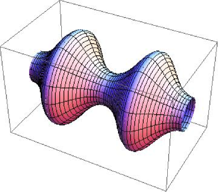
Figure 3: A graphical depiction of the non-uniform black cylinder based on the numerical evaluation of the blackfold equations for $n=1$ and $\nu=0.2$.

We will solve the differential equation (6.11) numerically, but some of the main properties of its solutions can be understood already by simple inspection. Rewriting (6.11) as

$$\frac{dR}{dz}=\pm\frac{1}{\nu_{n}-\nu}\sqrt{V_{\rm eff}(R)-(\nu_{n}-\nu)^{2}}~{},~{}~{}V_{\rm eff}(R)\equiv\Omega^{2}R^{2}(1-\Omega^{2}R^{2})^{n}$$ (6.13)

it becomes clear that there are non-uniform solutions with $R(z)$ oscillating between turning points of the equation where $R^{\prime}(z)=0$. At the turning points

$$V_{\rm eff}(R)=(\nu_{n}-\nu)^{2}~{}.$$ (6.14)

For all $n\geq 1$, there are always two turning points, $R_{-}<R_{+}$, between which $R$ oscillates with real first derivative provided the non-uniformity parameter $\nu$ lies in the interval $[0,\nu_{n}]$. At $\nu=0$ the turning points coalesce and one recovers the uniform solution (6.7). The oscillation amplitude becomes maximum at $\nu=\nu_{n}$ where $R_{-}=0$ and $R_{+}=\frac{1}{\Omega}$. In these solutions the thickness $r_{0}$ also oscillates according to eq. (6.6). It becomes maximum at $R_{-}$ and minimum at $R_{+}$. One should bear in mind that the blackfold approximation in principle breaks down near $R_{-}\approx 0$.

For each $\nu$ the period $L$ of the oscillation can be read easily from the differential equation (6.13). It is given by the integral expression

$$L=2\frac{\nu_{n}-\nu}{\Omega}\int_{\Omega R_{-}}^{\Omega R_{+}}dx\,\Big{[}x^{2}(1-x^{2})^{n}-(\nu_{n}-\nu)^{2}\Big{]}^{-\frac{1}{2}}~{}.$$ (6.15)

The dimensionless quantities $\Omega R_{\pm}$ depend only on $n$ and $\nu$.

To illustrate these properties more clearly let us consider in more detail the case $n=1$, i.e., a cylinder black membrane in $D=6$. In this case the turning points can be determined explicitly by solving a simple quadratic equation

$$\Omega R_{\pm}=\sqrt{\frac{1}{2}\pm\sqrt{\nu(\nu-1)}}~{}.$$ (6.16)

We can solve the differential equation (6.13) numerically to find the profile of $R(z)$ for any value of $\nu\in[0,\frac{1}{2})$. Fig. 3 is a three-dimensional graphical depiction of the solution for $n=1$ and $\nu=0.2$.

Figure 4: Plot of the velocity $\Omega R(z)$ based on numerical solutions of eq. (6.13) for $n=1$ and fixed $\kappa$ and $\Omega$ . Each curve represents $\Omega R(z)$ over a half-period. The curve oscillates between a minimum $R_{-}$ and a maximum $R_{+}$. The thick solid curve represents the uniform solution and has $\nu=0$. The remaining curves, starting from the solid one to the shorter-dashed ones, represent solutions with increasing values of $\nu$, respectively, $\nu=0.01,0.1,0.2,0.3,0.4$.

Fig. 4 depicts the result of the numerical evaluation over a half-period for six values of $\nu$ for fixed $\kappa$ and $\Omega$. As $\nu\to 0$ the profile of $R$ flattens and approaches that of the uniform solution. Also observe that the numerical value of the half-period ($\frac{\Omega L_{num}}{2}\sim 1.1$) compares well at $\nu=0.01$ with the perturbative value (6.10)

$$\frac{\Omega L_{pert}}{2}=\frac{\pi}{2\sqrt{2}}\sim 1.11072~{}.$$ (6.17)

As we increase $\nu$ the amplitude of $R$ increases and the period decreases. Short necks are forming at two points: $(i)$ near the minimum of $R$, where the diameter of the cylinder shortens, and $(ii)$ near the maximum of $R$, where the thickness $r_{0}$ diminishes. As $\nu$ approaches its upper bound, $\nu_{n}$, we enter a regime where the period $L(\nu)$ becomes comparable to $r_{0}$ and our blackfold approximations break down. What happens in this highly non-linear regime is an interesting problem.

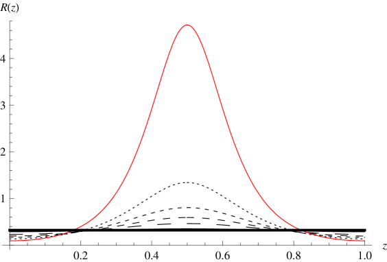
Figure 5: Plot of the radius $R(z)$ as a function of $z$ for fixed $L$ and angular momentum $J$, based on numerical solutions of eq. (6.13), (6.15), (6.18b) where we chose $n=1$, $L=1$, $J=1$ and $G=1$. The curve oscillates between a minimum $R_{-}$ and a maximum $R_{+}$. The thick solid curve represents the uniform solution and has $\nu=0$. The remaining curves, starting from the solid one to the shorter-dashed ones, represent solutions with increasing values of $\nu$, respectively, $\nu=0.01,0.1,0.2,0.3,0.4$. The red curve has $\nu=0.48$ and serves to illustrate what happens near extreme non-uniformity assuming the blackfold solution is trustworthy in that regime.

Another way of depicting these results is to plot $R(z)$ versus $z$ for fixed $L$. This is shown in Fig. 5. Naively, the infinite cylinder appears to reach a critical point where it breaks off into an array of ultra-spinning discs. This breaking-off reminds of the splitting of cylindrical streams of fluids into droplets under the Rayleigh-Plateau instability. A similar splitting of the horizon has been argued for non-uniform black strings [14]. We will return to this issue in the next subsection.

The mass, angular momentum and horizon area of these solutions can be computed using the general formulae. Defining these quantities per half-period we obtain the integral expressions

$$M=\frac{\pi\Omega_{(n+1)}}{4G}\left(\frac{n}{2\kappa}\right)^{n}\int_{0}^{\frac{L}{2}}(1-\Omega^{2}R^{2})^{\frac{n-2}{2}}(n+1-\Omega^{2}R^{2})R\sqrt{1+{R^{\prime}}^{2}}dz~{},$$ (6.18a)

$$J=\frac{\pi\Omega_{(n+1)}}{4G}\left(\frac{n}{2\kappa}\right)^{n}n\Omega\int_{0}^{\frac{L}{2}}(1-\Omega^{2}R^{2})^{\frac{n-2}{2}}R^{3}\sqrt{1+{R^{\prime}}^{2}}dz~{},$$ (6.18b)

$$A=4GS=4\pi\Omega_{(n+1)}\left(\frac{n}{2\kappa}\right)^{n+1}\int_{0}^{\frac{L}{2}}(1-\Omega^{2}R^{2})^{\frac{n}{2}}R\sqrt{1+{R^{\prime}}^{2}}dz$$ (6.18c)

which can be evaluated numerically.

In order to compare different solutions, it is also instructive to compute a set of dimensionless thermodynamic quantities defined as [3]

$$j=c_{j}\frac{J}{M(GM)^{\frac{1}{D-3}}}\sim\frac{\ell_{J}}{\ell_{M}}~{},~{}~{}a=c_{a}\frac{A}{(GM)^{\frac{D-2}{D-3}}}\sim\frac{A}{\ell_{M}^{D-2}}$$ (6.19)

where $c_{j}$ and $c_{a}$ are conveniently chosen constants. The $\kappa$ and $\Omega$ dependence of $M$, $J$ and $A$ follows easily by scaling. Accordingly, for any $\nu\in(0,\frac{1}{2})$ one can show that the dimensionless area of the cylindrical blackfolds behaves as

$$a=f(\nu,n)j^{-\frac{2}{n}}$$ (6.20)

where $f$ is a function of $\nu$ and $n$ that can be determined by solving the differential equation (6.13) and evaluating the integrals (6.18a)-(6.18c). We have performed this computation for several values of $n$. For $n=1$ the result has been plotted in fig. 6. As we increase $n$ the function $f$ develops a weak maximum at intermediate values of $\nu$, but other than that it retains the main qualitative features that are observed in fig. 6.

Figure 6: A plot of the product $aj^{2/n}$ as a function of $\nu$ based on the numerical solution of eq. (6.13) for $n=1$. $a$ and $j$ are respectively the dimensionless horizon area and angular momentum. The dots represent the outcome of the numerical computation with the choice $c_{j}=c_{a}=1$ in the definitions (6.19) of $a$ and $j$. The dashed line is an interpolation performed by mathematica. Near the right end of this plot $(\nu\sim 0.5)$ our approximations break down and our results should not be trusted.

6.2 Cylinders in Kaluza-Klein space

Compactifying one of the directions of the background and wrapping the cylindrical blackfold around it we obtain a black hole with compact horizon topology $(\widetilde{S}^{1}\times S^{1})\times s^{n+1}$. In terms of the parametrization (6.2) the KK $\widetilde{S}^{1}$ is labeled by

$$z\sim z+2\pi\widetilde{R}~{}.$$ (6.21)

Everything we said about cylindrical blackfolds in the previous subsection continues to hold in the compact case. The only difference comes from the constraints imposed by the periodicity relation (6.21). In particular, a non-uniform black cylinder can now fit in the KK direction if the KK circumference is an integer multiple of the period of the solution $L$, $i.e.$ if

$$2\pi\widetilde{R}=LN~{},~{}~{}N\in\mathbb{N}~{}.$$ (6.22)

Since $L$ is a function of $\nu,n$ (6.15), this implies a discretization of the allowed values of $\nu$. In what follows, we will fix $N$ and $\widetilde{R}$ (equivalently we fix $L$ from (6.22)) and consider how the thermodynamics vary in terms of the remaining parameters.

Figure 7: A plot of the rescaled horizon area $A/M^{\frac{n+2}{n}}$ as a function of the mass $M$ for uniform and non-uniform black cylinders on a KK space. The specific plot is based on a numerical evaluation of the stationary blackfold equations for $n=1$, $L=1$, $J=1$ and $G=1$. The uniform phase is represented by the solid horizontal line. The non-uniform phase is represented by the dashed line that emerges from the uniform branch at the critical mass $M\sim 6.49$.

With fixed $L$ the non-uniformity parameter $\nu$ becomes a function of $\Omega$. This function $\nu(\Omega)$ can be determined by inverting the relation (6.15). Then, $M$, $J$ and $A$ take the form

$$M=\frac{f_{M}\left(\nu(\Omega),n\right)}{G\kappa^{n}\Omega^{2}}~{},~{}~{}J=\frac{f_{J}\left(\nu(\Omega),n\right)}{G\kappa^{n}\Omega^{3}}~{},~{}~{}A=\frac{f_{A}\left(\nu(\Omega),n\right)}{G\kappa^{n+1}\Omega^{2}}$$ (6.23)

where $f_{M}$, $f_{J}$ and $f_{A}$ are functions of $\nu(\Omega),n$ that follow from the expressions (6.18a)-(6.18c). Using the second equation in (6.23) to re-express $\kappa$ in terms of $J$ we can write $M$ and $A$ as

$$M=\frac{f_{M}\left(\nu(\Omega),n\right)}{f_{J}\left(\nu(\Omega),n\right)}\Omega J~{},~{}~{}A=\frac{f_{A}\left(\nu(\Omega),n\right)}{\left[f_{J}\left(\nu(\Omega),n\right)\right]^{\frac{n+1}{n}}}\left(GJ\right)^{\frac{n+1}{n}}\Omega^{\frac{n+3}{n}}~{}.$$ (6.24)

The $J$-dependence of these expressions is explicit. The $\Omega$-dependence is more complicated and relies on the full solution of the stationary blackfold equations. A numerical evaluation of this dependence has been performed for several values of $n$ and the result is represented by the dashed curve in fig. 7 for $n=1$, $L=1$ and fixed $J=1$. For higher values of $n$, the curve continues to exhibit the same qualitative features.

The uniform phase is represented by a straight solid curve in fig. 7. Re-evaluating the thermodynamics (6.18a)-(6.18c) for the uniform cylinder (6.7) we find

$$A=f_{A,u}(n)M^{\frac{n+2}{n}}J^{-\frac{1}{n}}L^{-\frac{1}{n}}$$ (6.25)

where $f_{A,u}$ is the $n$-dependent coefficient

$$f_{A,u}(n)=\frac{8n}{n+2}\left(\frac{\Gamma\left(1+\frac{n}{2}\right)2^{n+2}(n+1)^{\frac{n+1}{2}}}{n^{\frac{2n}{2}}\pi^{2+\frac{n}{2}}(n+2)^{2}}\right)^{\frac{1}{n}}~{}.$$ (6.26)

The non-uniform branch is emerging from this phase at a critical value of $M$ ($M\sim 6.49$ for $n=1$, $L=1$, $J=1$) and evolves towards smaller entropy and mass. The last data point with $M\sim 1.52$ has $\nu=0.4$. As $\nu$ approaches its upper bound $\nu_{1}=0.5$ the gradients of the solution increase and our approximations break down. In the case of $N=1$, a single blob of the non-uniform solution (see fig. 5) is wrapping the $\tilde{S}^{1}$ direction $z$. Near the lower end of the non-uniform branch the solution shows a clear trend towards pancaking around a point of the circle into a disc configuration with vanishing $r_{0}$ at the edges. We analyzed such configurations in Section 5 where we argued that they represent the ultraspinning regime of spherical horizon Myers-Perry black holes. Hence, it seems appropriate to conjecture that the non-uniform branch continues towards a topology-changing merger point where it meets the localized branch of an ultraspinning Myers-Perry black hole in KK space. This picture is further motivated by the corresponding phase diagram of black holes and strings in KK spaces (see [16] for a review and references). In the present case, the blackfold approach has enabled us to reduce the problem to a simple first order differential equation like (6.13) that allows a straightforward analysis of a large part of the non-uniform branch.

7 Static minimal blackfolds

If the blackfold is static then its velocity field is

$$u=\frac{1}{R_{0}}\xi\,,$$ (7.1)

where $\xi$ is the timelike Killing vector of a static background. The intrinsic equations are trivially satisfied with $r_{0}=nR_{0}/2\kappa$. Let us assume that $R_{0}=1$. Then $u$ is a unit-normalized Killing vector and therefore its orbits are geodesics. In this case eq. (2.2) implies that $u^{\mu}u^{\nu}{K_{\mu\nu}}^{\rho}=0$ and the equations (2.1) for a perfect fluid become

$$Ph^{\mu\nu}{K_{\mu\nu}}^{\rho}=PK^{\rho}=0\,.$$ (7.2)

Since the local fluid pressure $P$ is always non-zero for a blackfold, the mean curvature vector $K^{\rho}$ must vanish. Hypersurfaces that satisfy this condition are called minimal, which is a bit of a misnomer since it is only guaranteed that they are extremal. In any case we will refer to the corresponding black brane configurations as minimal blackfolds.

Minimal surfaces are an intense field of study in mathematics and have a wide range of applications. Here we discover that they can also be relevant in the context of higher-dimensional black holes and branes. Regularity implies that the worldvolume of static blackfolds spans a sufficiently regular and non-intersecting minimal spatial submanifold. Many interesting examples of such embedded minimal surfaces are known and can be used as the basis for the construction of interesting black hole configurations. For instance, until fairly recently the only known minimal surfaces embedded in three dimensions were surfaces of revolution in

$$ds^{2}=dz^{2}+dr^{2}+r^{2}d\phi^{2}$$ (7.3)

describing the plane,

$$z=\mathrm{const}\,,$$ (7.4)

the helicoid

$$r=R\,,\qquad\phi=kz$$ (7.5)

and the catenoid

$$r=R\cosh(z/R)\,.$$ (7.6)

In 1982 Costa discovered a new minimal surface without self-intersections. This is a non-compact surface with genus one and three punctures. Since then more examples have been discovered. They all provide new solutions for static non-compact black branes.

In Euclidean space there can be no compact embedded minimal surfaces. Therefore it is not possible to construct a blackfold that gives a new asymptotically flat static black hole. This is indeed consistent with the theorem proved in [18] that the only such solution in higher-dimensional vacuum gravity is the Schwarzschild-Tangherlini black hole. All static neutral blackfolds in a Minkowski background are therefore non-compact.

8 Summary of horizon topologies and entropy ranking

In previous sections we presented a number of different solutions to the neutral blackfold equations. Table 1 summarizes the new types of asymptotically flat neutral black holes that arise from the blackfold analysis of the previous sections. With a possible M-theory motivation in mind we have included a list of horizon topologies in $D\leq 11$ dimensions that we have so far found to be allowed.

The list of Table 1 is only exhaustive of all possible black hole topologies in $D=5$ [29, 30] (barring the possibility of a regular black lens [31, 32, 33]), where in fact we have obtained all possible blackfold solutions. But it provides already a useful glimpse into the intricate structure of the phase space of higher-dimensional black holes.

$D=4$	$D=5$	$D=6$	$D=7$	$D=8$	$D=9$	$D=10$	$D=11$
$S^{2}$	$S^{3}$	$S^{4}$	$S^{5}$	$S^{6}$	$S^{7}$	$S^{8}$	$S^{9}$
		${B}_{2}\otimes s^{2}$	${B}_{2}\otimes s^{3}$	${B}_{2}\otimes s^{4}$	${B}_{2}\otimes s^{5}$	${B}_{2}\otimes s^{6}$	${B}_{2}\otimes s^{7}$
				${B}_{4}\otimes s^{2}$	${B}_{4}\otimes s^{3}$	${B}_{4}\otimes s^{4}$	${B}_{4}\otimes s^{5}$
						${B}_{6}\otimes s^{2}$	${B}_{6}\otimes s^{3}$
	$S^{1}\times s^{2}$	$S^{1}\times s^{3}$	$S^{1}\times s^{4}$	$S^{1}\times s^{5}$	$S^{1}\times s^{6}$	$S^{1}\times s^{7}$	$S^{1}\times s^{8}$
		$\mathbb{T}^{2}\times s^{2}$	$\mathbb{T}^{2}\times s^{3}$	$\mathbb{T}^{2}\times s^{4}$	$\mathbb{T}^{2}\times s^{5}$	$\mathbb{T}^{2}\times s^{6}$	$\mathbb{T}^{2}\times s^{7}$
			$S^{3}\times s^{2}$	$S^{3}\times s^{3}$	$S^{3}\times s^{4}$	$S^{3}\times s^{5}$	$S^{3}\times s^{6}$
			$\mathbb{T}^{3}\times s^{2}$	$\mathbb{T}^{3}\times s^{3}$	$\mathbb{T}^{3}\times s^{4}$	$\mathbb{T}^{3}\times s^{5}$	$\mathbb{T}^{3}\times s^{6}$
				$S^{1}\times S^{3}\times s^{2}$	$S^{1}\times S^{3}\times s^{3}$	$S^{1}\times S^{3}\times s^{4}$	$S^{1}\times S^{3}\times s^{5}$
					$\mathbb{T}^{4}\times s^{3}$	$\mathbb{T}^{4}\times s^{4}$	$\mathbb{T}^{4}\times s^{5}$
						$S^{5}\times s^{3}$	$S^{5}\times s^{4}$
						$\mathbb{T}^{2}\times S^{3}\times s^{3}$	$\mathbb{T}^{2}\times S^{3}\times s^{4}$
							$\mathbb{T}^{5}\times s^{4}$
						$S^{1}\times S^{5}\times s^{2}$	$S^{1}\times S^{5}\times s^{3}$
						$S^{3}\times S^{3}\times s^{2}$	$S^{3}\times S^{3}\times s^{3}$
							$\mathbb{T}^{3}\times S^{3}\times s^{3}$
							$S^{7}\times s^{2}$
							$\mathbb{T}^{2}\times S^{5}\times s^{2}$
							$S^{1}\times S^{3}\times S^{3}\times s^{2}$

Table 1: A partial list of possible horizon topologies for asymptotically flat neutral black holes in $D=4$ to $D=11$ dimensions based on the currently available solutions of the corresponding blackfold equations. $B_{2k}$ in the second row denotes the $2k$-dimensional filled-ellipsoids of Section 5 that appear in the blackfold description of ultraspinning MP black holes. $\otimes$ denotes a warped product geometry so the topologies in the second row are actually the same as in the first row. Capital (small) letters denote the part of the horizon with comparatively larger (smaller) characteristic scales.

The first row includes the exactly known Kerr black hole in four dimensions (the only phase allowed by uniqueness theorems), and its higher-dimensional generalizations, the MP black holes. The second row, which begins from $D=6$ and goes up, includes the possible ultraspinning limits of the MP black holes as even-ball blackfolds of the corresponding dimensionality. The topology of the horizons in the first and second row are therefore the same. The third row describes black ring solutions in any dimension $D\geq 5$. The five-dimensional black ring solution is known exactly [36]. In higher dimensions black ring solutions have been constructed perturbatively in the ultraspinning limit [3]. In this row one can also package the new less symmetric helical black rings that we presented in Section 3. The fourth row comprises of black two-tori. A perturbative solution for the metric of this type of black holes appears in appendix C. In subsequent rows increasingly complicated black holes appear with horizon geometries that include both tori and odd spheres. In previous sections we focused on round odd-sphere solutions with equal angular momenta, but we pointed out that solutions with unequal angular momenta are also possible (for a preliminary discussion see appendix A). They should also be included in this list. Not surprisingly, as we increase the spacetime dimension an increasingly larger set of possibilities opens up.

The physical properties of the new solutions can be computed in the ultraspinning limit using the blackfold methodology. It is interesting to compare the properties of different solutions, $e.g.$ their entropies. Under the assumption that the sizes of the compact directions in ${\cal{B}}_{p}$ are all of the same order $R$, it was shown in great generality in [2] that, for fixed mass, the rescaled entropy $s$ scales with the dimensionless angular momentum $j$ as

$$s(j)\sim j^{-\frac{p}{D-p-3}}~{}.$$ (8.1)

This scaling relation shows that for a given number of ultra-spins, the blackfold with smallest $p$ is the one that is entropically favored. Physically, objects with smaller values of $p$ are thicker at given mass and hence cooler. Since the entropy at constant mass is inversely proportional to the temperature, it follows that thicker objects, with lower $p$, have higher entropy. It must be recalled that an MP black hole with $k$ ultraspins is not to be regarded as a $0$-fold, but rather as a $2k$-fold.

Accordingly, the most entropic solutions among blackfolds with the same number of ultra-spins are black rings, which will be helical if more than one ultra-spin is involved. Since the helical ring with the shortest length is entropically favored, the helical ring with maximal entropy is the $n=(1,2,...,p)$ configuration, as discussed in Section 3.3.

9 Multiple black holes from blackfolds

The blackfold approach allows to easily construct multi-black hole configurations. Since the gravitational interaction of the blackfold is neglected to leading order, one simply superposes several blackfolds in a given configuration. As long as the separation between them is larger than $r_{0}$ (the largest of the thicknesses involved), a solution is obtained if all the blackfolds involved solve separately the blackfold equations.

These solutions often possess moduli and therefore are particularly sensitive to corrections from gravitational backreaction. For instance, it is obvious that two parallel flat branes solve the leading order, test-brane approximation, but they will attract and move towards each other as soon as the gravitational interaction is turned on. This is because the distance between the branes is a modulus and changing the distance does not break any symmetry. In contrast in a black Saturn with a central black hole and a surrounding black ring, the configuration does not admit any deformation of the relative position of the two objects that does not break any of its symmetries. Thus, when gravitational interaction is turned on, the gravitational energy will be extremized in the symmetric configuration and the configuration will remain in equilibrium (although presumably an unstable one).

Black Saturns [37] are the simplest configurations that can be obtained in this way, and indeed were analyzed in this manner in [38]. They admit generalizations involving the different new solutions we have found. For instance, a circular black ring may be surrounded (but not linked) by a helical black ring. The entire configuration also admits a central black hole. Observe that the black holes involved in these configurations can only rotate in the Killing directions that are not broken by the helical ring. In dimensions $D\geq 7$ an odd-sphere blackfold can be in stationary equilibrium with a central black hole, or with other concentrical blackfolds. Multiple blackfolds, each one lying in an independent submanifold of the background, which generalize the bicycle black rings of [41, 42], are also possible.

In this discussion the values of the temperature and angular velocities can be different among the several blackfolds involved. At the classical level, there is no problem in having, say, a central black hole and a surrounding black ring with different temperatures and angular velocities. However, in some instances, e.g., close to a merger between phases, the equality of these quantities among different objects is relevant. In ref. [3] it was suggested that ‘pancaked black Saturns’ in $D\geq 6$ consisting of a central ultraspinning black hole and a surrounding black ring might exist with equal angular velocities and temperatures, and could provide a way of connecting different phases.

We now argue that this is not the case. Focusing on the case with a single spin, an ultraspinning black hole corresponds to a blackfold disk, and the black ring to a circular string. If the rotation velocity is for both of them $\Omega$, then the radii of the two objects are related as

$$R_{\mathrm{ring}}=\frac{1}{\sqrt{D-4}\,\Omega}<R_{\mathrm{disk}}=\frac{1}{\Omega}\,,$$ (9.1)

(cf. (4.9) with $p=1$, $n=D-4$ for the ring, and (5.4) with $k=1$ for the disk). The inequality is strict since $n\geq 2$, so the circular ring would have to be inside the disk. Therefore the configuration is impossible, and ultraspinning black holes cannot be in full thermodynamical equilibrium with a surrounding black ring. As a consequence, the dashed phases and connections in figure 6 of ref. [3] cannot be realized, at least when the spin is sufficiently large.

10 Discussion and open problems

In this paper we have studied new stationary configurations of neutral black holes in dimension $D\geq 5$ by regarding them as thin black branes that wrap a submanifold of a background spacetime. The effective worldvolume theory that describes the long-wavelength dynamics of the black brane was formulated very generally in [2], and is quite similar to the effective Dirac-Born-Infeld theory for D-branes in open string theory, or the Nambu-Goto effective description for Nielsen-Olesen vortices. In our opinion, the blackfold approach should be regarded and judged in much the same way as one does in the case of these other effective theories, both in terms of its validity and of its utility. Blackfolds provide the leading order description of objects for which an exact account is very probably out of practical reach. Corrections to this leading order are more often than not very complicated too, but unless there is good reason to do so, one does not doubt the validity of this approximation to a full, physical solution describing the object in the complete theory.

There is however one significant respect in which blackfolds differ from DBI branes or NG strings (or indeed any other dynamical branes that we are aware of): the worldvolume theory of blackfolds features proper hydrodynamical behavior, in the sense of requiring local thermodynamical equilibrium. In contrast, NG strings have constant energy density and pressure, so their intrinsic dynamics is trivial, while the worldvolume dynamics of DBI branes is a nonlinear electrodynamics that does not involve thermal features. This is the main reason that in the blackfold theory configurations in stationary equilibrium are particularly singled out.

We hope the results of this paper demonstrate that this is indeed a powerful tool for the identification of new solutions and their properties. But its utility should not be reduced to only describing novel classes of stationary black holes, but also to analyzing their dynamics in specific physical situations. We now discuss these issues as well as some interesting directions for future research that this approach opens up.

The metric at all length scales

The blackfold approach as pursued in this paper might be regarded with scepticism since, although it is claimed that new black holes are found, no explicit black hole metric appears to be produced. Expressed in this crude form, this criticism is unwarranted. First, let us emphasize again the similarity to the fact that in general a solution of the DBI action does not provide an explicit solution to the full open string theory (indeed quite often it is not even known how to solve string theory in the backgrounds where this effective theory is applied), and a similar situation occurs for vortex strings and their Nambu-Goto description. Second, it is not quite true that no metric for the new black hole is given. It actually is, to leading order: far from the black hole, it is the background metric, with a submanifold singled out as the location of the blackfold; and near the black hole, it is the metric of a boosted black brane.

Nevertheless we admit that there is a point in this criticism, since traditionally black holes have been regarded as embodying a non-trivial geometry, and it might be desirable to see how a new metric is obtained for the new black hole, at least in principle. Indeed the first application of the blackfold methodology included a long and detailed analysis of the next-to-leading order metric for higher-dimensional black rings [3]. In appendix C we perform this analysis for black tori of general dimension.

As explained in detail in [3] (following [43, 44]) and [2], the method of matched asymptotic expansions (MAE’s) systematically produces an explicit solution for the geometry of the black hole spacetime at all scales, including the region near the horizon, with the effects of the bending of the black brane in an expansion in $r_{0}/R$. It should be appreciated that the leading order MAE is a rather involved technical task even in the very symmetric situations that we have studied, a fact that emphasizes once again the virtue of having a universal, long-distance effective theory that captures in a simple manner most of the physically interesting features of the solution.

Nevertheless, it would be interesting, and possibly quite informative, to perform a MAE in less symmetric examples where $r_{0}$ is a non-trivial function of the worldvolume coordinates. The even-ball blackfolds that describe the ultraspinning regime of MP black holes is such an example.

It would also be very interesting to go beyond the leading order in effective field theory and MAE’s. In the effective field theory side this would require a systematic derivation of the blackfold equations which would go beyond the leading order approximations to account for the effects of dissipation, internal structure and gravitational self-force. From the point of view of MAE’s one would have to setup a general expansion scheme as in [44].

The phase diagram of higher-dimensional black holes

We have uncovered large new classes of higher-dimensional black hole solutions in a specific ultraspinning regime (see table 1 for a partial list in $4\leq D\leq 11$ dimensions). The new solutions are part of a multi-dimensional ‘phase diagram’ where we can plot solutions at a fixed spacetime dimension with the axes being their asymptotic charges and entropy. In this diagram there are generically regions where several phases co-exist with the same asymptotic charges providing new examples of black hole non-uniqueness in higher-dimensional gravity. Indeed we have shown that helical black rings give rise to an infinite non-uniqueness, labelled by rational parameters, in all ultraspinning regions of the phase diagram. In these regions, helical black rings have the highest entropy among phases with connected horizons.

It would be very interesting to see how the new phases place themselves into the general phase diagram and to trace them away from the blackfold regime towards the non-linear regime of dynamics where different phases typically merge. Obtaining analytic information about the non-linear regime is a daunting task, but it may be possible to obtain valuable information by targeting specific examples numerically.

A more mundane task would be to aim for a qualitative global picture of the phase diagram extrapolating away from the available phases on the basis of well educated assumptions. Ref. [3] provides an example of such an approach. In that paper the discussion was limited to higher-dimensional black holes with a single spin. It would be desirable to generalize it to the case of black holes with more angular momenta and obtain a similar picture that involves the new solutions presented in this paper.

Another example of such extrapolations was briefly discussed in section 6.2 in the context of black cylinders in KK space. In fig. 7 we can track the behavior of the non-uniform ultraspinning black cylinder branch by solving the blackfold equations up to a point where a thin neck appears in the blackfold worldvolume geometry and our approximations break down. In the same phase diagram one expects an additional curve that describes an ultraspinning MP black hole localized in the KK direction. It would be interesting to determine the thermodynamics of this phase for small mass in perturbation theory. A natural expectation, which is corroborated by the behavior of the non-uniform black cylinder solutions in Section 6.2, is that there is a topology-changing merger point where the non-uniform black cylinder branch meets the localized MP branch.

Dynamical aspects: Stability and time-dependence

Many of the emerging new solutions of higher-dimensional gravity exhibit regions of instability in the blackfold regime. For example, ultraspinning MP black holes and thin black rings have been argued [25] to be unstable under GL-type instabilities. Corresponding statements can be made for more general blackfolds. As a matter of fact, the blackfold approach does easily capture this instability for a generic blackfold in a regime in which the wavelength $\lambda$ of the instability lies in the range $r_{0}\ll\lambda\ll R$. The instability appears in the intrinsic sector of the blackfold equations as an unstable sound mode of the effective worldvolume fluid [2].

This is one example where one can decouple the extrinsic equations from the stability analysis of the intrinsic sector. Conversely, there are situations where the extrinsic stability can be analyzed while guaranteeing that the intrinsic equations remain solved. A simple instance is the study of stability against variations of the radius of the round odd-sphere blackfolds of Sec. 4. These solutions extremize a potential $V=-I/\beta$ where $I$ is the action (4.8) for the stationary configurations. This $V$ is minimized by these solutions, implying that they are stable to variations of $R$ (this was in fact already known for black rings [45]). An explicit analysis of time-dependent perturbations confirms this result. This, and a more general investigation of instabilities and time-dependent physics for the new blackfold solutions presented in this paper will be discussed elsewhere.

Generating more solutions

The construction of higher-dimensional blackfolds in this paper was based on the black brane solution. It is possible to generalize this construction in several interesting ways. Internal ultra-spins along the transverse $(n+1)$-sphere, with rotation parameter $a\propto J/M\gg r_{0}$ can be incorporated by using the MP black branes as the starting point of the construction. Small internal spins, with $a\mathrel{\raisebox{-3.44444pt}{$\stackrel{{\scriptstyle\textstyle<}}{{\sim}}$}}r_{0}$, can also be incorporated easily to leading order since their effects only enter at a higher order in the expansion in $r_{0}/R$. An element of novelty is introduced by the zero-modes that appear at discrete values of the rotation [46] which, when present, should be included as part of the set of collective coordinates of the blackfold.

In general, the formalism can be applied easily to any brane whose effective stress tensor is known. One example are blackfolds based on the ‘lumpy’ black branes of [47, 48], which are black brane solutions branching off the regular black brane branch at the threshold of the GL mode. The resulting solutions, coined ‘lumpy blackfolds’ in [2], have horizons that are inhomogeneous on the small scale $r_{0}$.

Another set of interesting examples arises with blackfolds based on black branes constructed out of the exactly known black ring solution in five dimensions by adding extra flat dimensions to the metric. Such a ringy black string is in fact the exact solution that corresponds to the six-dimensional uniform black cylinder of Sec. 6. Bending it on a transverse $S^{1}$ in six dimensions will produce a blackfold with horizon topology $S^{2}\times S^{1}_{ring}\times S^{1}_{extra}$. With generic spin along $S^{1}_{ring}$ the new solution can now probe a different regime of the ultraspinning $\mathbb{T}^{2}$-blackfolds of Section 4.2. Several generalizations of this construction can be envisioned.

As explained in [2], essentially the same formalism as in this paper can be employed to study neutral blackfolds in any background with characteristic length scale $\gg r_{0}$, independently of what theory the background is a solution to as long as it contains the Einstein-Hilbert sector. With charged blackfolds the situation is different and will be discussed in detail elsewhere. One can use the approach, for example, to uncover new single- or multi-charged black hole solutions in supergravity theories that arise in 10D string theory or 11D M theory and their compactifications. These will be discussed in a future work.

Appendix A General equations for stationary black $S^{3}$-folds

In this appendix we consider the general equations for stationary blackfolds with horizon topology

$$S^{3}\times s^{n+1}~{}.$$ (A.1)

We embed the spatial part of the blackfold worldvolume, ${\cal B}_{3}$, in a four-dimensional subspace of $\mathbb{R}^{D-1}$ whose metric we parametrize as

$$d\rho^{2}+\rho^{2}(d\theta^{2}+\sin^{2}\theta d\phi^{2}+\cos^{2}\theta d\psi^{2})~{},~{}~{}0\leq\theta\leq\frac{\pi}{2}~{},~{}~{}0\leq\phi,\psi<2\pi~{}.$$ (A.2)

${\cal B}_{3}$ is wrapped around the three-sphere with coordinates $(\theta,\phi,\psi)$ and its embedding in $\mathbb{R}^{4}$ is provided by the radial scalar $\rho=R(\theta)$. Allowing for rigid rotation along the Killing directions associated with the angles $\phi$ and $\psi$, the velocity field $u$ is oriented along the Killing vector

$${\bf k}=\frac{{\partial}}{{\partial}t}+\Omega_{1}\frac{{\partial}}{{\partial}\phi}+\Omega_{2}\frac{{\partial}}{{\partial}\psi}~{}.$$ (A.3)

Consequently,

$$R_{0}=1~{},~{}~{}V(\theta)^{2}=R(\theta)^{2}(\Omega_{1}^{2}\sin^{2}\theta+\Omega_{2}^{2}\cos^{2}\theta)~{}.$$ (A.4)

The thickness $r_{0}$ is also a function of $\theta$

$$r_{0}(\theta)=\frac{n}{2\kappa}\sqrt{1-R(\theta)^{2}(\Omega_{1}^{2}\sin^{2}\theta+\Omega_{2}^{2}\cos^{2}\theta)}~{}.$$ (A.5)

With these data the stationary blackfold action (2.12) becomes

$$I(R)=\int_{0}^{\frac{\pi}{2}}d\theta\,\sin\theta\cos\theta R(\theta)^{2}\sqrt{R(\theta)^{2}+R^{\prime}(\theta)^{2}}\Big{(}1-R(\theta)^{2}(\Omega_{1}^{2}\sin^{2}\theta+\Omega_{2}^{2}\cos^{2}\theta)\Big{)}^{\frac{n}{2}}~{}.$$ (A.6)

Varying with respect to $R(\theta)$ we obtain the equation of motion

$$-(n-2)\Omega_{+}\Omega_{-}R^{2}R^{\prime}(R^{2}+{R^{\prime}}^{2})-2\cos(2\theta)\Big{(}-1+(\Omega_{+}^{2}+\Omega_{-}^{2})R^{2}\Big{)}(R^{2}+{R^{\prime}}^{2})R^{\prime}$$

$$+\sin(2\theta)R\Big{(}-4{R^{\prime}}^{2}+R(R^{\prime\prime}+R(-3+(\Omega_{+}^{2}+\Omega_{-}^{2})((n+3)R^{2}+(n+4){R^{\prime}}^{2}-RR^{\prime\prime})))\Big{)}$$

$$+(n+2)\Omega_{+}\Omega_{-}\cos(4\theta)R^{2}R^{\prime}(R^{2}+{R^{\prime}}^{2})$$

$$-\Omega_{+}\Omega_{-}\sin(4\theta)R^{3}\Big{(}(n+3)R^{2}+(n+4){R^{\prime}}^{2}-RR^{\prime\prime}\Big{)}=0~{}.$$ (A.7)

We have defined

$$\Omega_{\pm}=\frac{1}{2}(\Omega_{1}\pm\Omega_{2})~{}.$$ (A.8)

Setting $\Omega_{-}=0$ and $R=$constant in (A) we recover easily the round sphere solution of Subsection 4.1 with

$$R=\sqrt{\frac{3}{n+3}}\frac{1}{\Omega_{+}}$$ (A.9)

which is in exact agreement with eq. (4.9) for $p=3$.

It is an interesting problem to find inhomogeneous solutions of eq. (A) with $\Omega_{\pm}\neq 0$. It appears that numerical analysis will be needed for this task. We will not pursue this task here, but will exhibit a perturbative inhomogeneous solution for finite $\Omega_{+}$ and small $\Omega_{-}$.

Setting

$$R(\theta)=\sqrt{\frac{3}{n+3}}\frac{1}{\Omega_{+}}+\Omega_{-}r(\theta)~{},~{}~{}\Omega_{-}\ll\Omega_{+}$$ (A.10)

we expand the differential equation (A) to leading order in $\Omega_{-}$, solve for $r(\theta)$ and find the following inhomogeneous solution for generic $n$

$$R(\theta)=\sqrt{\frac{3}{n+3}}\frac{1}{\Omega_{+}}-\frac{3\sqrt{3(n+3)}}{n-9}\frac{\Omega_{-}}{\Omega_{+}^{2}}\cos(2\theta)+{\cal O}(\Omega_{-}^{2})~{}.$$ (A.11)

The values $n=1$ and $n=9$ appear to be special. For $n=1$ we find a one-parameter family of regular solutions at this order

$$R(\theta)=\frac{\sqrt{3}}{2}\frac{1}{\Omega_{+}}+\frac{3\sqrt{3}}{4}\frac{\Omega_{-}}{\Omega_{+}^{2}}\cos(2\theta)+c\Omega_{-}\Big{(}1+3\cos(4\theta)\Big{)}+{\cal O}(\Omega_{-}^{2})$$ (A.12)

where $c$ is a free parameter whose physical meaning is unclear. For $n=9$ we do not find a regular solution. It would be interesting to clarify these peculiarities and obtain a better understanding of these solutions numerically beyond perturbation theory.

Appendix B Physical magnitudes for even-ball blackfolds and ultraspinning MP black holes

B.1 Even-balls

Inserting the velocity field

$$V^{2}=\sum_{i=1}^{k}\Omega_{i}^{2}r_{i}^{2}$$ (B.1)

and (5.6) into (2.13), (2.14), (2.15) we find

$$M=\frac{r_{+}^{n}\Omega_{(n+1)}}{16\pi G}(2\pi)^{k}\int_{{\cal E}}\prod_{\ell=1}^{k}dr_{\ell}~{}r_{\ell}\left(n+1-\sum_{i}\Omega_{i}^{2}r_{i}^{2}\right)\left(1-\sum_{i}\Omega_{i}^{2}r_{i}^{2}\right)^{\frac{n}{2}-1}~{},$$ (B.2a)

$$J_{i}=\frac{nr_{+}^{n}\Omega_{(n+1)}}{16\pi G}(2\pi)^{k}\int_{{\cal E}}\prod_{\ell=1}^{k}dr_{\ell}~{}r_{\ell}r_{i}\left(1-\sum_{\ell}\Omega_{\ell}^{2}r_{\ell}^{2}\right)^{\frac{n}{2}-1}\Omega_{i}r_{i}~{},$$ (B.2b)

$$S=\frac{r_{+}^{n+1}\Omega_{(n+1)}}{4G}(2\pi)^{k}\int_{{\cal E}}\prod_{\ell=1}^{k}dr_{\ell}~{}r_{\ell}\left(1-\sum_{\ell}\Omega_{\ell}^{2}r_{\ell}^{2}\right)^{\frac{n}{2}}~{}.$$ (B.2c)

We have denoted the range of the $k$-dimensional integration as

$${\cal E}=\{\vec{r}~{}:~{}r_{i}\geq 0~{},~{}\sum_{\ell}\Omega_{\ell}^{2}r_{\ell}^{2}\leq 1\}~{}.$$ (B.3)

By changing variables to

$$x_{i}=\Omega_{i}r_{i}$$ (B.4)

we convert the range of integration to a piece of a unit $k$-ball, which we will denote as ${\cal E}_{1}$ (it would be a unit $k$-ball if $r_{i}$ were allowed to be both positive and negative). Thus, we get

$$M=\frac{r_{+}^{n}\Omega_{(n+1)}}{16\pi G}\prod_{\ell=1}^{k}\left(\frac{2\pi}{\Omega_{\ell}^{2}}\right)\int_{{\cal E}_{1}}\prod_{\ell=1}^{k}dx_{\ell}~{}x_{\ell}\left(n+1-\sum_{\ell}x_{\ell}^{2}\right)\left(1-\sum_{\ell}x_{\ell}^{2}\right)^{\frac{n}{2}-1}~{},$$ (B.5a)

$$J_{i}=\frac{nr_{+}^{n}\Omega_{(n+1)}}{16\pi G}\prod_{\ell=1}^{k}\left(\frac{2\pi}{\Omega_{\ell}^{2}}\right)\Omega_{i}^{-1}\int_{{\cal E}_{1}}\prod_{\ell=1}^{k}dx_{\ell}~{}x_{\ell}x_{i}^{2}\left(1-\sum_{\ell}x_{\ell}^{2}\right)^{\frac{n}{2}-1}~{},$$ (B.5b)

$$S=\frac{\Omega_{(n+1)}}{4G}r_{+}^{n+1}\prod_{\ell=1}^{k}\left(\frac{2\pi}{\Omega_{\ell}^{2}}\right)\int_{{\cal E}_{1}}\prod_{\ell=1}^{k}dx_{\ell}~{}x_{\ell}\left(1-\sum_{\ell}x_{\ell}^{2}\right)^{\frac{n}{2}}~{}.$$ (B.5c)

To compute these integrals we set

$$x_{i}=r\mu_{i}~{},$$ (B.6)

where $\mu_{i}$ are $k$ director cosines for $S^{k-1}$ spheres and $r\in[0,1]$. Then, integrals of the form

$$\int_{{\cal E}_{1}}\prod_{\ell=1}^{k}dx_{\ell}~{}x_{\ell}f\left(\sum_{\ell}x_{\ell}^{2}\right)$$

become

$$\int_{0}^{1}dr\,r^{2k-1}f(r^{2})~{}\int^{\prime}d\Omega_{(k-1)}\prod_{j=1}^{k}\mu_{j}~{},$$

where the prime over the sphere integral stands to remind us that we should not forget to impose the constraint $r_{i}\geq 0$.

Notice that we can decompose the metric of a $(2k-1)$-sphere as

$$d\Omega_{(2k-1)}^{2}=d\Omega_{(k-1)}^{2}+\sum_{i=1}^{k}\mu_{i}^{2}d\psi_{i}^{2}~{}.$$ (B.7)

We can deduce from here that

$$\int^{\prime}d\Omega_{(k-1)}\prod_{\ell=1}^{k}\mu_{\ell}=\frac{\Omega_{(2k-1)}}{(2\pi)^{k}}~{}.$$ (B.8)

To determine $J_{i}$ we use the following formula based on symmetry

$$\int_{{\cal E}_{1}}\prod_{\ell=1}^{k}dx_{\ell}~{}x_{\ell}x_{i}^{2}f\left(\sum_{j}x_{j}^{2}\right)=\frac{1}{k}\int_{{\cal E}_{1}}\prod_{\ell=1}^{k}dx_{\ell}~{}x_{\ell}\left(\sum_{j}x_{j}^{2}\right)f\left(\sum_{j}x_{j}^{2}\right)~{}.$$ (B.9)

With this and (B.8) we obtain the simple expressions (5.5a)-(5.5c) for the mass, angular momenta and area.

B.2 Ultraspinning MP black holes

Consider a Myers-Perry black hole in $D$ dimensions, with $k$ non-vanishing angular momenta. The solution is parametrized in terms of a mass parameter $\mu$ and $k$ rotation parameters $a_{i}$. The mass, angular momenta and angular velocities are

$$M=\frac{D-2}{16\pi G}\Omega_{(D-2)}\mu\,,$$ (B.10a)

$$J_{i}=\frac{2}{D-2}Ma_{i}\,,$$ (B.10b)

$$\Omega_{i}=\frac{a_{i}}{r_{+}^{2}+a_{i}^{2}}\,.$$ (B.10c)

The properties of the horizon, such as the radius $r_{+}$, surface gravity and area cannot be easily found for generic parameters, but they simplify dramatically in the ultraspinning limit in which [25]

$$a_{i}\gg\mu^{1/(D-3)}$$ (B.11)

(we assume $a_{i}>0$ without loss of generality). Then

$$r_{+}\to\left(\frac{\mu}{\prod_{i=1}^{k}a_{i}^{2}}\right)^{1/(D-2k-3)}\,,$$ (B.12)

and

$$\kappa\to\frac{D-2k-3}{2r_{+}}\,,$$ (B.13)

$$S\to\frac{\Omega_{(D-2)}}{4G}r_{+}^{D-2k-2}\prod_{i=1}^{k}a_{i}^{2}\,.$$ (B.14)

Then, substituting

$$\Omega_{(D-2)}=\frac{2\pi^{\frac{D-1}{2}}}{\Gamma(\frac{D-1}{2})}$$ (B.15)

into (B.10a) we obtain

$$M\to\frac{r_{+}^{D-2k-3}}{8G}\frac{(D-2)\pi^{\frac{D-3}{2}}}{\Gamma\left(\frac{D-1}{2}\right)}\prod_{i=1}^{k}a_{i}^{2}\,.$$ (B.16)

Also in this limit,

$$\Omega_{i}\to\frac{1}{a_{i}}\,.$$ (B.17)

The horizon has a round sphere $S^{D-2k-2}$ in directions transverse to the rotation planes with radius

$$R(S^{D-2k-2})\to r_{+}\cos\theta$$ (B.18)

where $\theta$ is a polar angle (more precisely, if the rotating directions are parametrized using direction cosines $\mu_{i}$, then $\sum_{i=1}^{k}\mu_{i}^{2}=\sin^{2}\theta$).

If we now set $n=D-2k-3$ and identify the angular velocities and surface gravity of this solution with those of a $2k$-ball blackfold (so $r_{+}$ is indeed the same in both constructions), then the expressions for the mass, angular momenta, and entropy (5.5a)-(5.5c), and radius of the transverse spheres (5.7) are exactly reproduced.

Appendix C Matched asymptotic expansions for black tori

In this appendix we present the main steps of a matched asymptotic expansion (MAE) that determines the full metric to leading order in the expansion parameter $r_{0}/R$ of rotating black tori in arbitrary spacetime dimension. This analysis generalizes the corresponding solutions of perturbative black rings in [3]. It provides perturbative black hole solutions with horizon topology $\mathbb{T}^{p}\times s^{n+1}$, for generic $p,n$ (satisfying $p\leq n+2$) and confirms that the horizon remains regular when the stationary blackfold equations are satisfied.

C.1 A note on coordinate systems

In order to study the effects of wrapping a black $p$-brane around an orthogonal $p$-dimensional torus $\mathbb{T}^{p}$ with radii $R_{i}$ ($i=1,\ldots,p$) it is convenient to introduce coordinates appropriately adapted to the torus. The asymptotic spacetime is $D$-dimensional Minkowski spacetime with $D=n+p+3$. We write its metric in the following coordinate system

$$ds^{2}_{D}=-dt^{2}+\sum_{i=1}^{p}\left(dr_{i}^{2}+r_{i}^{2}d\psi_{i}^{2}\right)+\sum_{k=1}^{n+2-p}dx_{k}^{2}~{}.$$ (C.1)

We envision wrapping the black $p$-brane around the surface parametrized by the toric angles $\psi_{i}$ at $r_{i}=R_{i}$ and $x_{k}=0$.

It is useful to define the radial coordinate $r$ and the director cosines $\mu_{a}$, $a=1,\ldots,n+2$, such that

$$r_{i}=R_{i}+r\mu_{i}~{},~{}~{}i=1,\ldots,p~{},~{}~{}~{}~{}x_{k}=r\mu_{p+k}~{},~{}~{}k=1,\ldots,n+2-p$$ (C.2)

with

$$\sum_{a=1}^{n+2}\mu_{a}^{2}=1~{},~{}~{}\sum_{a=1}^{n+2}d\mu_{a}^{2}=d\Omega_{(n+1)}^{2}~{}.$$ (C.3)

In the near-object limit, where $R_{i}\to\infty$ with $r$, $\mu_{a}$, $z_{i}=R_{i}\psi_{i}$ fixed, the Minkowski metric becomes

$$ds^{2}_{D}\simeq-dt^{2}+dr^{2}+r^{2}d\Omega_{(n+1)}^{2}+\sum_{i=1}^{p}\left(1+2\frac{r\mu_{i}}{R_{i}}\right)dz_{i}^{2}+{\cal O}\left(\frac{r^{2}}{R_{i}^{2}}\right)~{}.$$ (C.4)

It is also convenient to introduce another coordinate system, call it $r$-adapted coordinate system, for which the new $r$-coordinate defines scalar equipotential surfaces, $i.e.$ $\nabla^{2}r^{-n}=0$, to leading order in $1/R_{i}$. The leading order transformation that defines this system is (for $i=1,\ldots,p$, $k=1,\ldots,n+2-p$)

$$r\to r-\frac{r^{2}}{2n}\sum_{j=1}^{p}\frac{\mu_{j}}{R_{j}}~{},~{}~{}\mu_{i}\to\mu_{i}-\frac{r}{2n}\left(\mu_{i}\sum_{j=1}^{p}\frac{\mu_{j}}{R_{j}}-\frac{1}{R_{i}}\right)~{},~{}~{}\mu_{k+p}\to\mu_{k+p}\left(1-\frac{r}{2n}\sum_{j=1}^{p}\frac{\mu_{j}}{R_{j}}\right)~{}.$$ (C.5)

In these coordinates the Minkowski metric becomes

$$ds^{2}_{D}\simeq-dt^{2}+\left(1-\sum_{i=1}^{p}\frac{2r\mu_{i}}{nR_{i}}\right)\left(dr^{2}+r^{2}d\Omega_{(n+1)}^{2}\right)+\sum_{i=1}^{p}\left(1+\frac{2r\mu_{i}}{R_{i}}\right)dz_{i}^{2}+{\cal O}\left(\frac{r^{2}}{R_{i}^{2}}\right)~{}.$$ (C.6)

C.2 The far-zone

The first step of a MAE is to find a solution of a thin black $p$-torus, with $s^{n+1}$ radius $r_{0}\ll R_{i}$, in the far-zone, $r\gg r_{0}$, where the linearized approximation to gravity is valid.

We solve the linearized Einstein equations in transverse gauge,

$$\Box\bar{h}_{\mu\nu}=-16\pi GT_{\mu\nu}$$ (C.7)

with $\bar{h}_{\mu\nu}=h_{\mu\nu}-\frac{1}{2}h^{\rho}_{\rho}g_{\mu\nu}$ and $\nabla_{\mu}\bar{h}^{\mu\nu}=0$. $h_{\mu\nu}$ is the linear perturbation of the background metric $g_{\mu\nu}$. The source should be chosen to have support on a $p$-torus at $r_{i}=R_{i}$, $x_{k}=0$. Locally it should reproduce the stress-energy tensor of a boosted black $p$-brane solution. Choosing the critical boost for which the stationary blackfold equations, $T_{ii}=0$, are satisfied we obtain

$$T_{tt}=\frac{\Omega_{(n+1)}}{16\pi G}(n+p+1)r_{0}^{n}\prod_{i=1}^{p}\delta(r_{i}-R_{i})\delta(x_{k})~{},$$ (C.8a)

$$T_{ti}=\frac{\Omega_{(n+1)}}{16\pi G}\sqrt{n+p}\,r_{0}^{n}\prod_{i=1}^{p}\delta(r_{i}-R_{i})\delta(x_{k})~{},$$ (C.8b)

$$T_{ii}=0~{},~{}~{}T_{ij}=\frac{\Omega_{(n+1)}}{16\pi G}r_{0}^{n}\prod_{i=1}^{p}\delta(r_{i}-R_{i})\delta(x_{k})~{},~{}~{}i\neq j~{}.$$ (C.8c)

To integrate the equation (C.7) we use the Green’s function in $\mathbb{R}^{D-1}$

$$G(x,x^{\prime})=-\frac{1}{(D-3)\Omega_{(D-2)}}\frac{1}{|x-x^{\prime}|^{D-3}}~{}.$$ (C.9)

Notice that the stationary blackfold equations, $T_{ii}=0$, which are equivalent to the conservation of the stress-energy tensor, are necessarily satisfied in the transverse gauge.

It is now possible to obtain explicit integral expressions for the metric perturbation. Here we are mainly interested in the form of these expressions in the near-object limit that was defined below eq. (C.3). The form of the metric in this regime will provide boundary conditions for the near-zone metric of the next subsection. In the $r$-adapted coordinate system, and in Schwarzschild gauge

$$r\to r-\frac{1}{2n}\frac{r_{0}^{n}}{r^{n-1}}~{},$$ (C.10)

the far-zone metric perturbation reads

$$g_{tt}=-1+\frac{n+p}{n}\frac{r_{0}^{n}}{r^{n}}~{},$$ (C.11a)

$$g_{ti}=\frac{\sqrt{n+p}}{n}\frac{r_{0}^{n}}{r^{n}}\left(1+\frac{r\mu_{i}}{R_{i}}\right)~{},$$ (C.11b)

$$g_{i\neq j}=\frac{1}{n}\frac{r_{0}^{n}}{r^{n}}\left(1+\frac{r\mu_{i}}{R_{i}}+\frac{r\mu_{j}}{R_{j}}\right)~{},$$ (C.11c)

$$g_{ii}=1+\frac{1}{n}\frac{r_{0}^{n}}{r^{n}}\left(1+\frac{r\mu_{i}}{R_{i}}\right)+\frac{2r\mu_{i}}{R_{i}}~{},$$ (C.11d)

$$g_{rr}=1+\frac{r_{0}^{n}}{r^{n}}\left(1-\frac{2n-1}{n^{2}}\sum_{i=1}^{p}\frac{r\mu_{i}}{R_{i}}\right)-\frac{2}{n}\sum_{i=1}^{p}\frac{r\mu_{i}}{R_{i}}~{},$$ (C.11e)

$$g_{\Omega\Omega}=1+\frac{1}{n^{2}}\frac{r_{0}^{n}}{r^{n}}\sum_{i=1}^{p}\frac{r\mu_{i}}{R_{i}}-\frac{2}{n}\sum_{i=1}^{p}\frac{r\mu_{i}}{R_{i}}~{}.$$ (C.11f)

C.3 The near-zone

The next step requires solving the Einstein equations in the near-zone region, $r\ll R_{i}$. Here we are perturbing around the critically boosted black $p$-brane metric. Following the arguments of [3], we expect the perturbations to take the form

$$h_{\mu\nu}=\sum_{i=1}^{p}\frac{\mu_{i}}{R_{i}}a^{(i)}_{\mu\nu}(r)$$ (C.12)

Since the perturbations for each $i=1\ldots p$ will decouple to leading order in this expansion, we may consider for simplicity a given $i=k$. Hence, we perturb the critically boosted black $p$-brane in the following way

$$g_{tt}=-1+\frac{n+p}{n}\frac{r_{0}^{n}}{r^{n}}+\frac{\mu_{k}}{R_{k}}a(r)\,,$$ (C.13a)

$$g_{ti}=-\frac{\sqrt{n+p}}{n}\left[\frac{r_{0}^{n}}{r^{n}}+\frac{\mu_{k}}{R_{k}}b_{i}(r)\right]\,,$$ (C.13b)

$$g_{ij}=\delta_{ij}+\frac{1}{n}\frac{r_{0}^{n}}{r^{n}}+\frac{\mu_{k}}{R_{k}}c_{ij}(r)\,,$$ (C.13c)

$$g_{rr}=\left(1-\frac{r_{0}^{n}}{r^{n}}\right)^{-1}\left[1+\frac{\mu_{k}}{R_{k}}f(r)\right]\,,$$ (C.13d)

$$g_{\Omega\Omega}=1+\frac{\mu_{k}}{R_{k}}g(r)\,.$$ (C.13e)

By definition $g_{\Omega\Omega}$ multiplies the metric $r^{2}\sum_{j=1}^{n+2}d\mu_{j}^{2}$ of a $S^{n+1}$ of radius $r$. In the above formulae we have omitted for brevity a label $k$ on the functions $a$, $b_{i}$, $c_{ij}$, $f$ and $g$.

With this ansatz, the location of the horizon will remain at $r=r_{0}$ if the perturbations are finite there. This fixes partially the choice of radial coordinate, but there still remains some gauge freedom under the transformation

$$r \to r+\gamma(r)\,\frac{r_{0}}{R_{k}}\mu_{k}\,,$$ (C.14a)

$$\mu_{i} \to \mu_{i}+\beta(r)\,\frac{r_{0}}{R_{k}}(\mu_{i}\mu_{k}-\delta_{ik})$$ (C.14b)

with

$$\beta^{\prime}(r)=\frac{\gamma(r)}{r^{2}\left(1-\frac{r_{0}^{n}}{r^{n}}\right)}~{}.$$ (C.15)

With this change of coordinates the metric retains its form to leading order in $1/R_{k}$. The condition that the horizon stays at $r=r_{0}$, $i.e.$ $r_{0}\to r_{0}+O(1/R_{k}^{2})$, is

$$\gamma(r_{0})=0~{}.$$ (C.16)

In addition, there is an $r$-independent dipole gauge transformation,

$$\mu_{i}\to\mu_{i}+\beta_{0}\,\frac{r_{0}}{R_{k}}(\mu_{i}\mu_{k}-\delta_{ik})$$ (C.17)

with constant $\beta_{0}$ that leaves everything unchanged except for $g(r)$ which is redefined by an additive constant

$$g(r)\to g(r)+2r_{0}\beta_{0}~{}.$$ (C.18)

Let us summarize how many undetermined functions we have. Based on symmetry considerations we expect (again for fixed $k$) that

$$b_{k}=b\ ,\ \ b_{i\neq k}=\widetilde{b}\ ,\ \ c_{kk}=c\ ,\ \ c_{k,i\neq k}=\widetilde{c}\ ,\ \ c_{i\neq k,j\neq k}=\widehat{c}~{}.$$ (C.19)

The unknown functions are therefore $a,b,\widetilde{b},c,\widetilde{c},\widehat{c},f,g$. From these we can form the gauge-invariant combinations

$${\sf A}(r) = a(r)-(n+p)\,c(r)\,,$$ (C.20a)

$${\sf B}(r) = b(r)-n\,c(r)\,,$$ (C.20b)

$${\sf F}(r) = f(r)+2r_{0}\left(\frac{r^{n+1}}{r_{0}^{n+1}}\;c(r)\right)^{\prime}-\frac{n}{\left(1-\frac{r_{0}^{n}}{r^{n}}\right)}\;c(r)\,,$$ (C.20c)

$${\sf G}^{\prime}(r) = g^{\prime}(r)+2\frac{r_{0}}{r}\left(\frac{r^{n+1}}{r_{0}^{n+1}}\;c(r)\right)^{\prime}+\frac{2}{r\left(1-\frac{r_{0}^{n}}{r^{n}}\right)}\;c(r)\,$$ (C.20d)

$$\widetilde{\sf B}(r) = \widetilde{b}(r)-nc(r)\ ,\ \ \widetilde{\sf H}(r)=\widetilde{c}(r)-c(r)\ ,\ \ \widehat{\sf H}(r)=\widehat{c}(r)-c(r)~{}.$$ (C.20e)

The first four functions are the same as in the black ring case with $p=1$ [3]. For $p>1$ there are three additional functions.

The far-zone analysis (see (C.11)) imposes the following boundary conditions on these functions

$${\sf A}(r) = -2(n+p)\,r-\frac{n+p}{n}\frac{r_{0}^{n}}{r^{n-1}}+{\cal O}\left(r^{-n-1}\right)\,,$$ (C.21a)

$${\sf B}(r) = -2n\,r+{\cal O}\left(r^{-n-1}\right)\,,$$ (C.21b)

$${\sf F}(r) = 4(n+2)\frac{r^{n+1}}{r_{0}^{n}}+\frac{2}{n}(1-n^{2})r+{\cal O}\left(r^{-(n-1)}\right)\,,$$ (C.21c)

$${\sf G}^{\prime}(r) = 4(n+2)\frac{r^{n}}{r_{0}^{n}}+\frac{2}{n}(1+2n)+{\cal O}\left(r^{-n}\right)\ \,,$$ (C.21d)

$$\widetilde{\sf B}(r) = -2nr-\frac{r_{0}^{n}}{r^{n-1}}+{\cal O}\left(r^{-n-1}\right)\,,$$ (C.21e)

$$\widetilde{\sf H}(r) = -2r+O\left(r^{-n-1}\right)\,,$$ (C.21f)

$$\widehat{\sf H}(r) = -2r-\frac{1}{n}\frac{r_{0}^{n}}{r^{n-1}}+O\left(r^{-n-1}\right)~{}.$$ (C.21g)

We can now proceed to determine the gauge invariant functions by solving the Einstein equations. The computation simplifies considerably by noting that the boundary conditions (C.21) and the form of the Einstein equations depend non-trivially only on $n$, and that the $p$-dependence can be incorporated easily with appropriate rescalings.

From the $R_{r\theta}=0$ equation we can determine ${\sf F}(r)$ in terms of the other functions. $\theta$ is one of the angles parametrizing the director cosine $\mu_{k}$ that appears in the perturbation (C.13). Then, from linear combinations of the equations associated to $R_{tt},R_{rr},R_{\Omega\Omega}$ we can solve for the function ${\sf G}^{\prime}(r)$ in terms of the functions ${\sf A}(r)$, ${\sf B}(r)$, ${\sf B}(r)$, $\widetilde{\sf H}(r)$, $\widehat{\sf H}(r)$ and their first derivatives. The remaining equations simplify considerably if we define and substitute for the following auxiliary functions

$${\cal K}_{1}=2\widetilde{\sf H}-\widehat{\sf H}~{},~{}~{}{\cal K}_{2}=-n\widetilde{\sf H}+\widetilde{\sf B}~{},~{}~{}{\cal K}_{3}=\widetilde{\sf B}-n\widehat{\sf H}~{},$$ (C.22)

$${\cal M}={\sf B}-{\cal K}_{2}~{},~{}~{}\SS={\sf B}-{\cal K}_{3}~{},~{}~{}{\cal C}=(n+1)\left(-\frac{n}{n+p}{\sf A}+2{\sf B}\right)~{}.$$ (C.23)

The functions ${\cal K}_{1}$, ${\cal M}$ and ${\cal C}$ obey the same decoupled $p$-independent differential equation

$$-(n+1)r^{n-1}{\sf Y}+\left((n+1)r^{n}-r_{0}^{n}\right){\sf Y}^{\prime}+r\left(r^{n}-r_{0}^{n}\right){\sf Y}^{\prime\prime}=0~{}.$$ (C.24)

$\SS$ and ${\sf B}$ obey the differential equation

$$-(n+1)r^{n-1}{\sf X}+(n+1)\left(r^{n}-r_{0}^{n}\right){\sf X}^{\prime}+r\left(r^{n}-r_{0}^{n}\right){\sf X}^{\prime\prime}+n(n+1)r_{0}^{n}{\cal K}^{\prime}_{1}=0~{}.$$ (C.25)

From the first set of equations (C.24) and the boundary conditions (C.21) we deduce the simple linear relations

$${\cal C}(r)=(n+1){\cal M}(r)~{},~{}~{}{\cal M}(r)=n{\cal K}_{1}(r)~{}.$$ (C.26)

From (C.25) and the boundary conditions we deduce that

$$\SS(r)={\sf B}(r)~{}~{}\Leftrightarrow~{}~{}{\cal K}_{3}(r)=0~{}.$$ (C.27)

These equations are enough to determine the functions $\widetilde{\sf B}(r)$, $\widetilde{\sf H}(r)$, $\widehat{\sf H}(r)$ in terms of ${\sf A}(r)$, and ${\sf B}(r)$. We find

$$\widetilde{\sf H}(r)=\frac{1}{n}{\sf B}(r)~{},~{}~{}\widetilde{\sf B}(r)=\frac{n}{n+p}{\sf A}(r)~{},~{}~{}\widehat{\sf H}(r)=\frac{1}{n+p}{\sf A}(r)~{}.$$ (C.28)

Finally, we differentiate (C.24) (applied to ${\cal K}_{1}$) once with respect to $r$ and substitute for the derivatives of ${\cal K}_{1}$ the expression that follows from (C.25) in terms of ${\sf B}$. Then we get for ${\sf B}$ a fourth order master equation, the same equation that appeared for $p=1$ in [3] (eq. (6.16) in that paper). The master equation can be solved by a linear combination of hypergeometric functions (see [3] for details). Using the above equations the function ${\sf A(r)}$ can be expressed in terms of ${\sf B}(r)$ and its first, second and third derivatives (the relation is given by eq. (6.15) in [3] by replacing ${\sf B}\to\frac{n+1}{n+p}{\sf A}$ and ${\sf A}\to{\sf B}$). So, once we determine ${\sf B}$ all remaining functions are determined.

C.4 Matching and the complete solution

The boundary conditions (C.21) provide the matching between the far-zone and near-zone expansions. We can use them to solve the master equation for ${\sf B}$, then from ${\sf B}$ we can determine the other gauge invariant functions and finally we can fix the gauge to obtain the complete metric. The details of this exercise proceed mutatis mutandis to the black ring case that was analyzed in [3]. We refer the reader to that paper for further details. We remark here that since the perturbations are of dipole type the physical quantities do not receive modifications to order $1/R_{i}$. Moreover, as observed for the black ring family $S^{1}\times s^{n+1}$ in Ref. [3], the hypergeometric functions entering in the solution presented above simplify drastically for $n=1$. As a consequence, the first-order corrected metric is not only simpler for the five-dimensional black ring, but also for the horizon topologies $\mathbb{T}^{2}\times s^{2}$ and $\mathbb{T}^{3}\times s^{2}$ in six and seven dimensions respectively.

References

- [1] R. Emparan, T. Harmark, V. Niarchos, and N. A. Obers, World-volume effective theory for higher-dimensional black holes. (Blackfolds), Phys. Rev. Lett. 102 (2009) 191301, [0902.0427].
- [2] R. Emparan, T. Harmark, V. Niarchos and N. A. Obers, Essentials of Blackfold Dynamics, JHEP 1003, 063 (2010) [0910.1601].
- [3] R. Emparan, T. Harmark, V. Niarchos, N. A. Obers, and M. J. Rodriguez, The Phase Structure of Higher-Dimensional Black Rings and Black Holes, JHEP 10 (2007) 110, [0708.2181].
- [4] N. A. Obers, Black Holes in Higher-Dimensional Gravity, Lect. Notes Phys. 769 (2009) 211–258, [0802.0519].
- [5] V. Niarchos, Phases of Higher Dimensional Black Holes, Mod. Phys. Lett. A23 (2008) 2625–2643, [0808.2776].
- [6] R. Emparan and H. S. Reall, Black Holes in Higher Dimensions, Living Rev. Rel. 11 (2008) 6, [0801.3471].
- [7] M. M. Caldarelli, R. Emparan, and M. J. Rodriguez, Black Rings in (Anti)-deSitter space, JHEP 11 (2008) 011, [0806.1954].
- [8] J. Camps, R. Emparan, P. Figueras, S. Giusto, and A. Saxena, Black Rings in Taub-NUT and D0-D6 interactions, JHEP 02 (2009) 021, [0811.2088].
- [9] J. Le Witt and S. F. Ross, Black holes and black strings in plane waves, [0910.4332].
- [10] J. J. Blanco-Pillado, R. Emparan, and A. Iglesias, Fundamental Plasmid Strings and Black Rings, JHEP 01 (2008) 014, [0712.0611].
- [11] S. Hollands, A. Ishibashi, and R. M. Wald, A higher dimensional stationary rotating black hole must be axisymmetric, gr-qc/0605106.
- [12] V. Moncrief and J. Isenberg, Symmetries of Higher Dimensional Black Holes, Class. Quant. Grav. 25 (2008) 195015, [0805.1451].
- [13] H. S. Reall, Higher dimensional black holes and supersymmetry, hep-th/0211290.
- [14] H. Kudoh and T. Wiseman, Connecting black holes and black strings, Phys. Rev. Lett. 94 (2005) 161102, [hep-th/0409111].
- [15] B. Kol, The phase transition between caged black holes and black strings: A review, Phys. Rept. 422 (2006) 119–165, [hep-th/0411240].
- [16] T. Harmark, V. Niarchos, and N. A. Obers, Instabilities of black strings and branes, Class. Quant. Grav. 24 (2007) R1–R90, [hep-th/0701022].
- [17] T. Colding and W.P. Minicozzi, Minimal surfaces, Courant Lecture Notes in Mathematics, 4. New York University, Courant Institute of Mathematical Sciences, New York, 1999.
- [18] G. W. Gibbons, D. Ida, and T. Shiromizu, Uniqueness and non-uniqueness of static vacuum black holes in higher dimensions, Prog. Theor. Phys. Suppl. 148 (2003) 284–290, [gr-qc/0203004].
- [19] B. Carter, Essentials of classical brane dynamics, Int. J. Theor. Phys. 40 (2001) 2099–2130, [gr-qc/0012036].
- [20] D. Astefanesei, M. J. Rodriguez, and S. Theisen, Quasilocal equilibrium condition for black ring, JHEP 12 (2009) 040, [arXiv:0909.0008].
- [21] T. Harmark and N. A. Obers, General definition of gravitational tension, JHEP 05 (2004) 043, [hep-th/0403103].
- [22] D. Kastor, S. Ray, and J. Traschen, The first law for boosted Kaluza–Klein black holes, JHEP 06 (2007) 026, [arXiv:0704.0729 [hep-th]].
- [23] B. Carter, Stability and characteristic propagation speeds in superconducting cosmic and other string models, Phys. Lett. B228 (1989) 466–470.
- [24] B. Carter, Brane dynamics for treatment of cosmic strings and vortons, hep-th/9705172.
- [25] R. Emparan and R. C. Myers, Instability of ultra-spinning black holes, JHEP 09 (2003) 025, [hep-th/0308056].
- [26] V. Cardoso and O. J. C. Dias, Rayleigh-Plateau and Gregory-Laflamme instabilities of black strings, Phys. Rev. Lett. 96 (2006) 181601, [hep-th/0602017].
- [27] M. M. Caldarelli, O. J. C. Dias, R. Emparan, and D. Klemm, Black Holes as Lumps of Fluid, JHEP 04 (2009) 024, [0811.2381].
- [28] B. Kol and M. Smolkin, Classical Effective Field Theory and Caged Black Holes, Phys. Rev. D77 (2008) 064033, [0712.2822].
- [29] G. J. Galloway and R. Schoen, A generalization of Hawking’s black hole topology theorem to higher dimensions, Commun. Math. Phys. 266 (2006) 571–576, [gr-qc/0509107].
- [30] C. Helfgott, Y. Oz, and Y. Yanay, On the topology of black hole event horizons in higher dimensions, JHEP 02 (2006) 025, [hep-th/0509013].
- [31] S. Hollands and S. Yazadjiev, Uniqueness theorem for 5-dimensional black holes with two axial Killing fields, Commun. Math. Phys. 283 (2008) 749–768, [arXiv:0707.2775].
- [32] J. Evslin, Geometric Engineering 5d Black Holes with Rod Diagrams, JHEP 09 (2008) 004, [arXiv:0806.3389].
- [33] Y. Chen and E. Teo, A rotating black lens solution in five dimensions, Phys. Rev. D78 (2008) 064062, [arXiv:0808.0587].
- [34] T. Harmark, Domain Structure of Black Hole Space-Times, Phys. Rev. D80 (2009) 024019, [arXiv:0904.4246].
- [35] B. Kleihaus, J. Kunz, and E. Radu, static black holes with event horizon topology, Phys. Lett. B678 (2009) 301–307, [arXiv:0904.2723].
- [36] R. Emparan and H. S. Reall, A rotating black ring in five dimensions, Phys. Rev. Lett. 88 (2002) 101101, [hep-th/0110260].
- [37] H. Elvang and P. Figueras, Black saturn, JHEP 05 (2007) 050, [hep-th/0701035].
- [38] H. Elvang, R. Emparan, and P. Figueras, Phases of five-dimensional black holes, JHEP 05 (2007) 056, [hep-th/0702111].
- [39] H. Iguchi and T. Mishima, Black di-ring and infinite nonuniqueness, Phys. Rev. D75 (2007) 064018, [hep-th/0701043].
- [40] J. Evslin and C. Krishnan, The Black Di-Ring: An Inverse Scattering Construction, Class. Quant. Grav. 26 (2009) 125018, [0706.1231].
- [41] H. Elvang and M. J. Rodriguez, Bicycling Black Rings, JHEP 04 (2008) 045, [0712.2425].
- [42] K. Izumi, Orthogonal black di-ring solution, Prog. Theor. Phys. 119 (2008) 757–774, [0712.0902].
- [43] T. Harmark, Small black holes on cylinders, Phys. Rev. D69 (2004) 104015, [hep-th/0310259].
- [44] D. Gorbonos and B. Kol, A dialogue of multipoles: Matched asymptotic expansion for caged black holes, JHEP 06 (2004) 053, [hep-th/0406002].
- [45] H. Elvang, R. Emparan, and A. Virmani, Dynamics and stability of black rings, JHEP 12 (2006) 074, [hep-th/0608076].
- [46] O. J. C. Dias, P. Figueras, R. Monteiro, J. E. Santos, and R. Emparan, Instability and new phases of higher-dimensional rotating black holes, Phys. Rev. D80 (2009) 111701, [arXiv:0907.2248].
- [47] S. S. Gubser, On non-uniform black branes, Class. Quant. Grav. 19 (2002) 4825–4844, [hep-th/0110193].
- [48] T. Wiseman, Static axisymmetric vacuum solutions and non-uniform black strings, Class. Quant. Grav. 20 (2003) 1137–1176, [hep-th/0209051].