A Two-Colour CCD Survey of the North Celestial Cap:
I. The Method

Abstract

We describe technical aspects of an astrometric and photometric survey of the North Celestial Cap (NCC), from the Pole ($\delta=90^{\circ}$) to $\delta=80^{\circ}$, in support of the TAUVEX mission. This region, at galactic latitudes from $\sim 17^{\circ}$ to $\sim 37^{\circ}$, has poor coverage in modern CCD-based surveys. The observations are performed with the Wise Observatory one-meter reflector and with a new mosaic CCD camera (LAIWO) that images in the Johnson-Cousins R and I bands a one-square-degree field with sub-arcsec pixels. The images are treated using IRAF and SExtractor to produce a final catalogue of sources. The astrometry, based on the USNO-A2.0 catalogue, is good to $\sim$ 1 arcsec and the photometry is good to $\sim$0.1 mag for point sources brighter than R=20.0 or I=19.1 mag. The limiting magnitudes of the survey, defined at photometric errors smaller than 0.15 mag, are 20.6 mag (R) and 19.6 (I). We separate stars from non-stellar objects based on the object shapes in the R and I bands, attempting to reproduce the SDSS star/galaxy dichotomy. The completeness test indicates that the catalogue is complete to the limiting magnitudes.

1 Introduction

The North Celestial Cap Survey (hereafter NCCS) is compiled from digital imaging observations of the Northern Celestial Cap region ($\delta\geq+80^{\circ}$) performed at the Wise Observatory from February 13, 2009 with the 1-meter Boller and Chivens telescope and the Large Area Imager at Wise Observatory (LAIWO) digital camera. The NCCS is a photometric and astrometric catalogue in the Johnson-Cousins R and I bands (Johnson & Morgan, 1953; Cousins, 1974) and is expected to contain more than 1,500,000 distinct objects. This paper presents technical details of the project and a brief discussion of the quality of the first results.

The NCCS catalogue of point and extended objects supports the TAUVEX project. The TAUVEX space telescope array, constructed by ElOp (Electro-Optic Industries Ltd.), a division of ELBIT Systems, for Tel Aviv University with funding from the Israel Space Agency (Ministry of Science, Culture, and Sport), consists of a bore-sighted assembly of three 20-cm telescopes imaging in the vacuum UV the same $\sim$one-degree field of view from geosynchronous orbit. Satellites in such orbits and, in particular, those used for telecommunications, are normally not used for astronomy since they do not point-and-track celestial objects. To allow the observation of various objects in the sky TAUVEX is mounted on the side of the Indian Space Research Organization (ISRO) GSAT-4 satellite on a Mounting Deck Plate (MDP) that can aim the TAUVEX line of sight (LOS) to different declinations, from $\delta$=+90^∘ to $\delta$=-90^∘. As GSAT-4 orbits the Earth on its geo-synchronous orbit, the TAUVEX LOS scans a sky ribbon. The data transmitted to the ground station are reconstructed into a set of UV images of the sky ribbon scanned by the experiment.

The scanning mode of observation used by TAUVEX implies that the motion of objects through the TAUVEX field of view is done at the sidereal rate. Because of this, the exposure times for each source vary with declination $\delta$ as $\frac{1}{cos\delta}$. In order to reach very deep exposures without requiring numerous re-scans of the same sky ribbon, the TAUVEX observations will mostly be restricted to the circumpolar regions and, for the first half-year of the mission, the area to be observed will mainly be 90${}^{\circ}\leq|\delta|\leq 80^{\circ}$; the northern sky patch covered by NCCS.

TAUVEX in survey mode uses its three principal filters SF-1, SF-2 and SF-3. These filters span the spectral region from somewhat longer than Lyman $\alpha$ to 320 nm with three well-defined bands. Three filters define two color indices in the UV that can be combined with optical (e.g., V-R or R-I) and eventually infrared color indices to characterize the nature of detected sources.

The availability of visual and near-infrared photometric digital sky surveys from 1990’s, such as DSS, SDSS and 2MASS, made the process of retrieving astronomical data easy as never before and contributed greatly to the development of modern astronomy. Reshetnikov (2005) presented a very good review of sky surveys and deep fields. Yet, very few high-quality photometric data are available for the Northern Celestial Cap region. The NCCS aims to produce a catalogue of positions and R-I color indices to complement the UV colours obtained by TAUVEX.

The first high-quality digital sky survey, the Digitized Sky Survey (DSS), was produced by scanning the plates of photographic surveys (POSS-I, POSS-II, ESO/SERC) with specific photometric calibrations. Although the DSS and its extension DSS-II are both all-sky surveys and cover the North Celestial Pole region, they are based on photographic observations and suffer from photographic emulsion shortcomings, such as low sensitivity, limited dynamic range and non-linearity. The limiting magnitude of the survey also differs for different directions, depending on which photographic survey was used to retrieve the data (B${}_{lim}\cong 20.^{m}0$ for POSS-I, $\cong 22.^{m}5$ for POSS-II and $\cong 18.^{m}5$ for ESO/SERC).

Another great ccontribution of these photographic surveys (POSS-I, POSS-II, ESO/SERC) was to provide high-precision astrometry used in catalogues such as USNO-A1.0, USNO-A2.0, USNO-B1.0, etc. The USNO-A and USNO-B catalogues were all-sky high-precision astrometric catalogues including also photometric data. USNO-A included two-color (B and R) one-epoch data, while the USNO-B catalogue included three-color (B, R and I) and two-epoch data. The USNO-B1.0 catalogue included photometric data with an accuracy of 0.3 mag and astrometric data with an accuracy of 0.2 arcsec for more than a billion individual objects as faint as V$=21.^{m}0$ (Monet et al., 2003). The catalogue provided separation with 85% accuracy of stars and non-stellar objects with internal magnitudes $14\leq M_{V}\leq 20$. The USNO-B1.0 catalogue was released at the same time that the SDSS early data release became available. Monet et al. (2003) compared the two data sets and found “systematic offsets as large as 0.25 arcsec … taken as evidence for distortions of the USNO-B1.0 astrometric calibration”. Moreover, when transforming the catalogue magnitudes to SDSS magnitudes and comparing common objects, systematic photometric errors as high as 0.20 mag and dispersions up to 0.34 mag were found, which can be explained probably by the photographic nature of the catalogue.

Another digital sky survey is the Two Micron All Sky Survey (2MASS). 2MASS was performed in the near-infrared (NIR): J (1.25 $\mu$m), H (1.65 $\mu$m) and K_s (2.17 $\mu$m) with two robotic telescopes in the USA and Chile in 1997-2001. The NIR was chosen to minimize the influence of galactic and extragalactic dust on the photometric data. 2MASS is not suitable as a reference survey for the TAUVEX project by itself, since it is NIR only and is not sufficiently deep, with limiting magnitudes J = 15.8, 15.0 mag, H = 15.1, 14.3 mag and K_s = 14.3, 13.5 mag for point and extended sources respectively (Skrutskie et al., 2006).

The Sloan Digital Sky Survey (SDSS) covers about 10,000 square degrees of the sky and provides high-precision photometric data in five Sloan bands with limiting magnitudes of $u_{lim}=22.^{m}0$, $g_{lim}=22.^{m}2$, $r={lim}=22.^{m}2$, $i_{lim}=21.^{m}3$, $z_{lim}=20.^{m}5$ for point objects and an astrometric accuracy of $<0.^{\prime\prime}1$ RMS per coordinate (Abazajian et al., 2009). SDSS is not suitable as well for the TAUVEX project purposes, since it does not cover the North Celestial Cap, but will be used here for comparison, as a commonly accepted standard.

The NCCS is essential for the TAUVEX project since no available survey completely satisfies the requirements to support TAUVEX in this sky region. Here we describe the method, the achieved accuracy, and provide a comparison with SDSS. In a following paper we will present some preliminary results.

2 Observations

The observations were performed at the Wise Observatory, Israel, from February 13, 2009 in runs of 3-9 nights per month. The 1-meter telescope and the LAIWO camera were used. LAIWO is a mosaic CCD camera built at the Max Planck Institute for Astronomy, Heidelberg. The telescope and camera parameters are listed in Table 1.

Table 1: The Telescope and Camera Parameters:

Parameter	Value
Telescope
Clear aperture	101.6 cm
Focal length (f/7)	711.2 cm
Secondary mirror diameter	51 cm
Field of view	$\sim$4.9 square degrees
LAIWO
Number of CCDs	4 science + 1 guider
Nimber of pixels	4$\times$4096$\times$4096 (science)
Pixel size	15 $\mu$m
Field of view	$59^{\prime}\times 59^{\prime}$
Sampling	$\sim$0.′′44 per pixel
Peak quantum efficiency	$\sim$40% between 600 and 850 nm
Read-out noise	$9<$RON$<19$ e-
	(quadrant-dependent)
Full-well depth	$\sim$80,000 e-
Gain	5 e- ADU-1

The technical parameters of LAIWO determined during its construction were described by Baumeister et al. (2006). For a more detail description of LAIWO and its performance see Afonso et al. 2010, in prep. Nevertheless, we dedicate the following subsection to describe its characteristics and performance for a better understanding of the potential and adequacy of LAIWO for the NCCS survey.

2.1 LAIWO

The LAIWO camera consists of four Lockheed CCD486 4096$\times$4096 pixel frontside-illuminated devices, refered to as the science CCDs. The LAIWO observation manual and some technical details can be found in Kaspi (2009) and Afonso (2007). At the f/7 focus of the Wise telescope each pixel subtends 0.43 arcsec and each CCD images a 29.5$\times$29.5 arcmin² field. The CCDs are mounted on a single heat sink cooled by liquid nitrogen (lN₂) to -105$\pm 5^{\circ}$C and are individually connected to the lN₂ dewar with flexible copper bands. The chips are not contiguous, but are spaced $\sim$26 arcmin apart. Each science CCD is connected to four output channels to reduce the read-out time of the entire mosaic. Figure 1 shows the layout of the LAIWO 16 quadrants in North-East orientation. The resultant image of an exposure is a mosaic FITS file (Hanisch et al., 2001) consisting of 16 extensions.

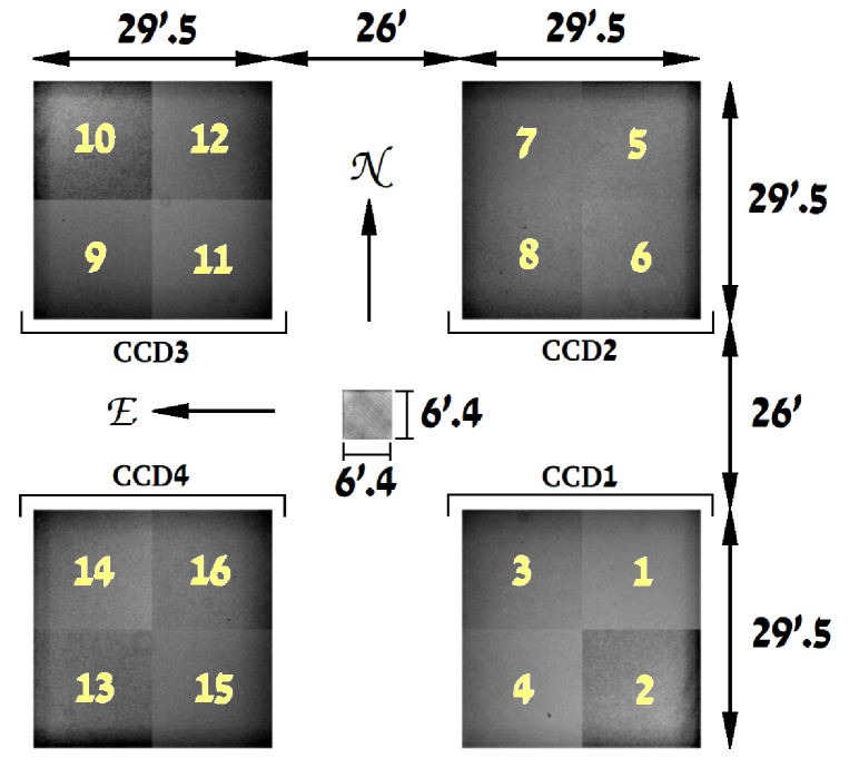
Figure 1: I band flat field imaged with LAIWO science CCDs on June 12, 2009 used to show LAIWO CCD layout. A clear-filter flat field imaged with LAIWO guider CCD on July 5, 2009 is shown at the center of the image. The relative sizes and distances are preserved.

The science CCDs exposures are binned 2$\times$2 to match the typical seeing, reducing the number of pixels to 16 Mpixel sampled to $\sim 0.^{\prime\prime}87$ arcsec per binned pixel. The read-out time of the entire mosaic in 2$\times$2 binning is only $\sim$28 sec.

A guider CCD is located at the center of the science CCDs mosaic. This is a back-illuminated e2V CCD47-20 device with 1024$\times$1024 13$\mu$m pixels, corresponding to 0.38 arcsec pixel^-1, with maximal quantum efficiency of $\sim$80% and covering a $6.^{\prime}4\times 6.^{\prime}4$ field of view. The science and the guider CCDs can be exposed separately and/or simultaneously. The guider CCD usually takes continuous short exposures of a small region including a guiding star. The image is compared to the previous one and, if the shift of the star photocenter exceeds certain limits, the telescope pointing is corrected via a LAIWO-telescope interface. The guider CCD images are not stored by default at the end of the night.

LAIWO has no dead or hot pixels, however all the flat field images taken with the camera have all the pixels in column X=1 and in row Y=1 saturated in each quadrant. Row Y=2 in each quadrant shows sometimes a few saturated pixels. Fig. 2 shows the World Coordinate System specific to each LAIWO quadrant. Note that the saturated columns X=1 and rows Y=1 in each LAIWO quadrant are the edge columns and the edge rows of each CCD; this saturation feature is not observed in science images. For this reason, sources located near the image edges are not extracted.

Figure 2: WCS defined for each LAIWO quadrant. The relative sizes and distances are not preserved here. The CCD identification and orientation are like in Fig. 1.

The entire LAIWO CCD array detects 1090$\pm$30 cosmic rays (CR) during a 300-sec exposure ($\sim$3.6 CR*sec^-1). Most CRs produce $\sim$100-300 counts above the background, with only $\sim$7% of the CRs produce more than 1,000 counts above the background. Table 2 shows the average numbers of the CRs detected in each CCD from four 300-sec exposures of the same field taken on May 14 and June 13, 2009.

Table 2: LAIWO CR Sensitivity:

	CR number
CCD #	Total	$>$ 1,000 counts
1	280$\pm$20	18$\pm$4
2	270$\pm$20	22$\pm$5
3	270$\pm$20	20$\pm$4
4	270$\pm$20	22$\pm$5
total	1090$\pm$30	80$\pm$10

The edge-to-center (EC) flat field (FF) ratio of LAIWO is about the same for the R and I bands and is $\sim 86\%$. Table 3 shows the EC values for each quadrant, extracted from twilight FF images from June 14, 2009. The center FF value was extracted as the mean value of the 16 pixels of the particular quadrant located near the CCD center. The edge value was extracted as the mean value of the 16 pixels furthest from the CCD.

Table 3: Edge-to-Center Flat Field Ratio of the LAIWO Camera:

	I-band Flat Field	R-band Flat Field
Quadrant #	Edge-to-Center Ratio	Edge-to-Center Ratio
1	84.9$\pm$0.7%	87.9$\pm$0.7%
2	90.9$\pm$0.7%	88.1$\pm$0.8%
3	86.6$\pm$0.7%	86.3$\pm$0.7%
4	88.3$\pm$0.7%	83.9$\pm$0.7%
5	84.6$\pm$0.7%	87.0$\pm$0.7%
6	84.8$\pm$0.7%	83.7$\pm$0.7%
7	84.8$\pm$0.7%	86.1$\pm$0.7%
8	86.3$\pm$0.7%	83.9$\pm$0.7%
9	84.8$\pm$0.7%	86.0$\pm$0.7%
10	93.8$\pm$0.7%	88.9$\pm$0.7%
11	83.0$\pm$0.7%	85.0$\pm$0.7%
12	87.6$\pm$0.7%	85.1$\pm$0.7%
13	88.8$\pm$0.7%	89.3$\pm$0.8%
14	88.0$\pm$0.7%	85.9$\pm$0.7%
15	85.4$\pm$0.7%	85.7$\pm$0.7%
16	87.3$\pm$0.7%	83.5$\pm$0.7%
Global average	87$\pm$3%	86$\pm$2%

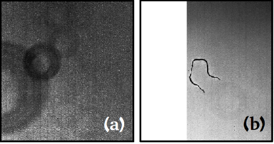
Figure 3: LAIWO dust difraction patterns. Panel (a) shows a donut pattern in I band flat field. Panel (b) shows a filament pattern in R band flat field.

The LAIWO camera FFs exhibit different obscuration patterns, which are divided into two groups: ring-shaped dust diffraction patterns (“donuts”) and irregular patterns (“filaments”). Fig. 3 shows examples of these patterns, observed on FFs from June 12, 2009. The donuts are produced by dust particles located on the filter or on the CCD window and affect the exposure level at a $\sim$1% level. Their location and number may vary from filter to filter and from night to night. The filaments are produced probably by dust particles or tiny debris located on the CCDs themselves. They dim the light by $\sim$20% and their location is constant for all the filters, but their number may change from night to night. These features are observed also in science images. We eliminate their influence by using FFs taken in the same night and by imaging the same sky field three times with dithering of $\sim$15^′′ , to prevent the appearance of the features on the final, debiased, FF-subtracted and median-combined image.

A 0-sec exposure of LAIWO camera shows a bias level of $\sim 400\pm 20$ counts pixel^-1 (hereafter 1 count = 1 ADU). A 300-sec dark exposure produces an additional dark level of $3\pm 3$ counts pixel^-1 ($\sim$0.01 counts pixel^-1 sec^-1). Bias/dark exposures taken at the beggining and at the end of a night show the same bias/dark levels.

Using SExtractor (Source-Extractor, SE; Bertin & Arnouts 1996), we obtained Kron (1980) aperture parameters for all the objects $2\sigma$ above the background noise from an image of the Landolt (2009) standard field SA107 taken on June 14, 2009 at an airmass of 1.175. The Kron aperture is an elliptical aperture fitted individually to every object. The parameters of Kron aperture are a, b and $\theta$, the semi-major and semi-minor axes and the position angle of the main axis, respectively. The a and b parameters of the Kron aperture are analogs of the FWHM of circular aperture.

By exposing this image at a low airmass we eliminate the effect of atmospheric dispersion which is further reduced by the filter bandpass restriction. The ellipticity of the objects may arise from an optical distortion, from some CCD tilt, from inaccurate tracking/guiding or from a combination of these factors. We divided every quadrant into 3$\times$3=9 regions and calculated the mean value of a, b and $\theta$ of the objects in them. The results are plotted in Fig. 4. In a number of quadrants the major axes are directed mostly from the camera center outwards. The exception is CCD2 (upper-right corner) where the ellipses seem to be directed almost randomly. Note that the ellipse elongation on the X axis is greater than that on Y axis.

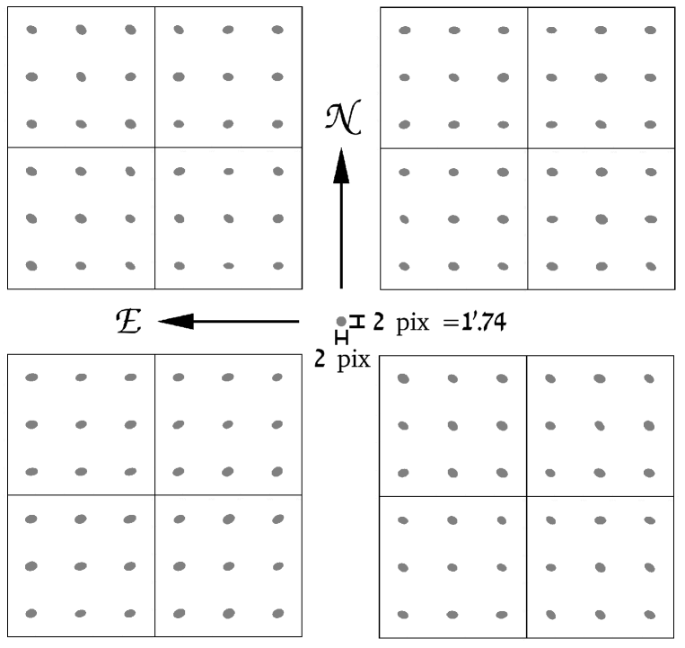
Figure 4: LAIWO distortion picture. The grey circle at the center is for scaling and shows an ideal circular object with FWHM 2”. The quadrant layout is as shown in Fig. 1.

2.2 Observational Strategy

The NCCS observational strategy is to obtain three 300-sec exposures of each field in the two Johnson-Cousins filters R and I, with a small $\sim$15^′′ dithering between the exposures. The three 300-sec exposures are then registered and median-combined to allow the detection of fainter objects and to reduce random noises such as sky and object Poisson noise, dust interference patterns, cosmic rays, satellite tracks, etc. Biases, 300-sec darks and twilight FFs are also taken at the beginning of each night. Landolt (2009) photometric standard stars are observed, usually during one night of the run, whenever the weather conditions allow. For runs when no Landolt standards are observed, the photometric calibrations are derived from the overlapping regions of the particular run and other runs.

The fields are chosen using two selection criteria. The first is that they should be as close to the meridian as possible and they should be higher than the North Celestial Pole to be observed at the lowest possible airmass. We try to follow the meridian during the night, however the hour angle deviation from the meridian may sometimes be up to $3^{h}$. The second criterion is that the following field should have a small overlap region with the previous field to provide a contiguous coverage of the NCC region, filling in the “empty” spaces between the CCDs in LAIWO array.

3 Data Reduction

The reductions are done using a fully-automated pipeline written in IRAF (Image Reduction and Analysis Facility; Tody 1986) script. The pipeline uses the SE program (Bertin & Arnouts, 1996) to obtain object fluxes from the images, and the WCSTools (World Coordinate Systems Tools) package of programs (Mink, 2002) to extract astrometric standards from USNO-A2.0 catalogue (Monet, 1998). The pipeline input consists of all the images of a particular night. The pipeline output is a list of objects containing the parameters defined in Table 4. Most of the data are extracted automatically by the SE routines. The pipeline runtime (including reductions, photometric and astrometric calibrations) is about 6 hours for one observing night.

Table 4: Pipeline Output Parameters:

#	Output Parameter	Remarks
1	Image date
2	Filter
3	Airmass
4	Quadrant number
5	Object number
6	Object position along X
7	Object position along Y
8	RA (J2000.0)
9	DEC (J2000.0)
10	Corrected isophotal flux
11	RMS error for ISOCORR flux
12	Kron flux
13	RMS error for Kron flux
14	Petrosian flux
15	RMS error for Petrosian flux
16	FWHM
17	Kron radius
18	Background level
19	Semi-major axis	of Kron apperture
20	Semi-minor axis	of Kron apperture
21	Position angle	of Kron apperture
22	Ellipticity	of Kron apperture
23	Elongation	of Kron apperture
24	SE internal flags
25	Truncation flag

The pipeline median-combines all the bias and dark exposures to obtain master bias and master dark frames. The master bias is subtracted from the FFs and the debiased FFs are median-combined with mode scaling to obtain master flat frames for the R and I bands. The master flats are normalized, each quadrant to its median. The master dark is subtracted from the science images and the dark-subtracted science images are then normalized by the master flats. The normalized science images are then split into 16 separate images, one per CCD quadrant, keeping the common WCS aligned (East to the left, North up).

All the images are grouped by the sky imaged field, by the number of the quadrant and by the filter. Each group contains three 300-sec debiased, dark-subtracted and flat-fielded exposures of the same quadrant in the same field, taken with the same filter. For each image in the group the shifts produced by dithering are calculated. The earliest taken image between the three is used as the reference frame. The images are then registered to cover exactly the same field. The images in each group are then median-combined to obtain one less noisy 300-sec exposure, as explained above. The resultant image contains only the overlapping region of the three original images; rows and columns out of the overlapping region are filled by the median value of the overlapping region.

The combined science images are scanned with SE. We prefer SE photometry to IRAF photometry since it is very fast and robust. We define the scanning threshold of the SE to be 2$\sigma$ above the noise fluctuations, which corresponds to a point-object detection probability of 95.4%.

We use Kron (1980) aperture photometry to determine the flux of the objects, which uses an elliptical adaptive aperture, for a number of reasons:

1. LAIWO produces elongated objects even at low airmass as shown in Fig. 4.

2. The survey area is relatively close to the horizon (Alt = $20^{\circ}-40^{\circ}$, airmass $\cong$ 2.0), therefore all point sources will be slightly elongated by the atmospheric dispersion. For point sources, this seems preferable to that of a circular aperture.

3. Elliptical apertures are natural for extended sources. Moreover, galaxy Kron fluxes can be easily transformed into Petrosian fluxes (Graham & Driver, 2005), which are used in the SDSS.

4. The Kron photometry is flexible, since the aperture is fitted individually to each object.

5. The Kron photometry provides additional parameters of the detected objects, such as semi-major and semi-minor axes, inclination angle, ellipticity and elongation. These parameters are very useful for star/galaxy separation and for field distortion estimation.

The SE subtracts the sky counts from the object counts. We set the background subtraction parameters of the SE to local background fit and subtraction. For each saturated object, or one that overlaps with another, has poor photometry, is truncated, etc. the SE ascribes an internal flag. The SE defines as truncated an object that is close to the edge of a quadrant, that may not necessarily be the edge of the common region of the three initial 300-sec exposures. The source lists need therefore to be cleared from false detections produced by objects located only partly in the common region of the combined image. The pipeline ascribes the truncation flag to all the objects located closer than 10 pixels to the edge of the common region of the combined images.

The pipeline also calculates the airmass of the image and the effective airmass of the combined 300-sec exposure, which we define as the mean airmass of the three initial exposures. The airmass that appears in the output lists is the effective airmass of the combined exposure.

4 Photometric calibration

The photometric calibration is relative to Landolt (2009) standards. Currently the photometric calibration program is not a part of the pipeline. Some modified parts of the pipeline and an adittional program written in MATLAB are used for photometric calibrations. If the standard data for a run are missing, we derive calibration equations from objects in the overlapping region between a particular run and another run when standards were observed.

The following calibration equations were obtained from the June 14, 2009 night. The Landolt SA107 field, which contains stars with R and I magnitudes of about $10^{m}-15^{m}$ and R - I colours from $-0.^{m}5$ to $+1.^{m}4$, was observed at 11 airmasses from 1.17 to 3.16 with 120-sec exposures. The calibration coefficients were obtained from the Kron fluxes of 18 standard stars. The following calibration equations were derived:

$$\begin{array}[]{rcl}R&=&-2.5\log(N_{R}/t)-(0.155\pm 0.006)X+(0.001\pm 0.042)(R-I)+(20.952\pm 0.023)\\ I&=&-2.5\log(N_{I}/t)-(0.092\pm 0.004)X+(0.349\pm 0.029)(R-I)+(19.743\pm 0.016)\end{array}$$ (1)

where $N/t$ is the object flux in ADU sec^-1 and $X$ is the airmass.

We define as ‘grey’ magnitudes $m_{I}$ and $m_{R}$ the object magnitudes obtained from equations (1) without including the colour term. We also define the instrumental colour $m_{R}-m_{I}$ as the difference between the grey magnitudes of the object in the respective filters. Using calibration equations (1), the relation between the instrumental and Landolt colours is:

$$\begin{array}[]{rcl}R-I&=&0.742(m_{R}-m_{I})\\ \Delta(R-I)&=&0.742\sqrt{\Delta m_{R}^{2}+\Delta m_{I}^{2}+(m_{R}-m_{I})^{2}(0.042^{2}+0.029^{2})}\end{array}$$ (2)

Equation (2) allows the transformation of fluxes to magnitudes in two stages, since the R and I images of the same field would not necessary be of exactly the same field due to small changes in telescope pointing and image dithering. The detected objects would not have exactly the same X and Y, and some would possibly miss I or R exposures till later stages of the survey. Moreover, one needs to know the true (R - I) colour of each object to perform the correction of magnitudes in equation (1) for the colour term, and the object true (R - I) colour is usually not known beforehead. Therefore, the photometric transformation needs to be done in two stages: first, to obtain the grey magnitudes from the fluxes, and second, after the astrometric solution for the field is found, to correct the grey magnitudes for the colour terms, using colours obtained from equation (2). This yields the true R and I magnitudes of the objects.

Fig. 5 shows the Landolt colours vs. the calculated instrumental colours and the line predicted from equation (2). The fit of the photometric solution in equation (1) to the magnitudes ofthe Landolt standards has a root-mean-square error $\sigma=0.047$ mag and $\sigma=0.033$ mag in the R and I bands respectively.

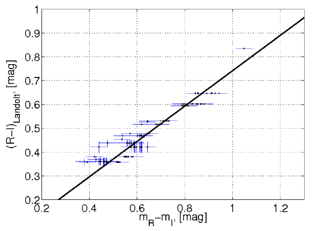
Figure 5: Landolt colour vs. Instrumental colour. The black solid line shows the relation predicted by the equation (2).

5 Astrometric calibration

Since the telescope pointing is not sufficiently accurate, an astrometric solution needs to be found for every field. For the astrometric calibration we use the USNO-A2.0 catalogue, which contains entries for more than half a billion stars with an accuracy of $\sim$0.25 arcsec and covers the entire sky (Monet, 1998). We use the WCSTools package to extract the needed part of the catalogue. The J2000.0 $(\alpha,\delta)$ coordinates of the extracted part of the catalogue are then transformed to the (X, Y) plane coordinates using the center of the LAIWO array as a tangential point. The brightest unsaturated stars with $SNR\geq 1,000$ in each LAIWO quadrant are extracted by the SE and the quadrant output lists are combined into the CCD output lists to obtain a more accurate solution. The number of the stars used for the astrometric solution in each CCD is usually $\sim$30.

The (X, Y) coordinates of the brightest stars are matched with the (X, Y) coordinates of the extracted catalogue part using the downhill simplex algorithm (Nelder & Mead, 1965). The algorithm produces an initial match between the coordinate lists with an accuracy of $\sim$10-14 pixels. The final astrometric solution is then fitted by IRAF using a tangetial projection with parabolic surfaces and a linear distortion along the X and Y axes. The J2000.0 $(\alpha,\delta)$ coordinates of each object are calculated and updated in the output lists. The final RMS deviation of the NCCS astrometric data for the most of fields ranges from 0.5 to 0.8 arcsec and is in all the cases better than 1.25 arcsec in both RA and DEC. The astrometry was tested also against SDSS; the results are presented in Section 8 below.

6 Limiting Magnitudes

Following the derivation of the astrometric solution and the correction of the grey magnitudes for the colour terms, the true R and I magnitudes are calculated for each object. Once the transformation operations are performed we can estimate the photometric accuracy and depth of our survey. The saturation limit derived from the images on June 14, 2009 is R = 11.5 mag and I = 11.5 mag for a 300-sec exposure. Figs. 6 and 7 show the Kron R and I magnitude errors as a function of Kron R and I magnitudes respectively for $\sim$10,000 objects from the same field imaged on June 12, 2009. The objects were extracted from a 300-sec combined exposure adopting a minimal SNR = 2. Table 5 shows the R and I magnitudes extracted from Figs. 6 and 7 that correspond to median errors of 0.05, 0.10 and 0.15 mag.

Table 5: R and I Magnitudes Corresponding to the Values of R and I Errors:

$\Delta$R, $\Delta$I	R	I
0.05	18.6	17.8
0.10	20.0	19.1
0.15	20.6	19.6

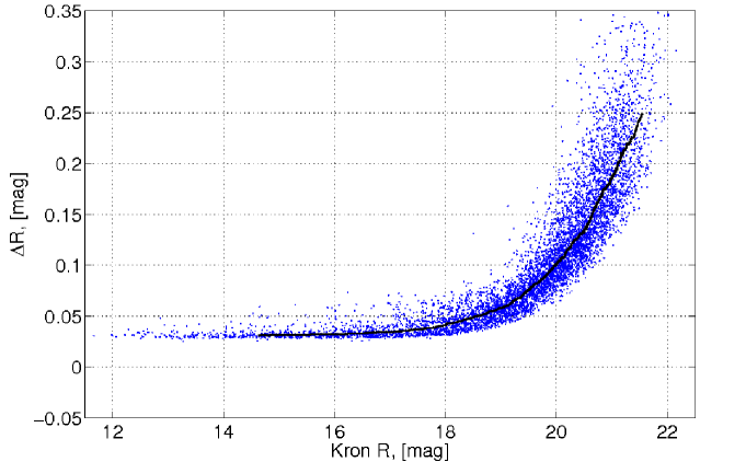
Figure 6: Kron R magnitude errors as a function of Kron R magnitudes for $\sim$10,000 objects imaged in the same field. The black line shows a running median of errors in 400-object bins.

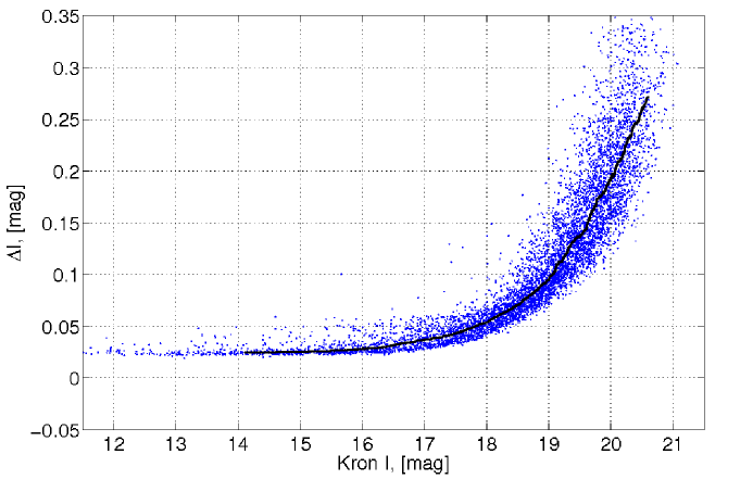
Figure 7: Kron I magnitude errors as a function of Kron I magnitudes for $\sim$10,000 objects imaged in the same field. The black line shows a running median of errors in 400-object bins.

Excluding all the sources with R $>$ 20.6 mag and I $>$ 19.6, we expect that the RMS error of the (R - I) colour should be smaller than $(0.15)\times\sqrt{2}\cong 0.2$ mag. Fig. 8 shows the (R - I) colour errors as a function of (R - I) colour for $\sim$4,000 objects brighter than R = 20.6 and I = 19.6 mag, extracted from the same 300-sec combined exposure as in Figs. 6 and 7. The median of the colour errors is $\cong 0.1$ mag for colour indices $-0.25\leq(R-I)\leq 2.2$. We therefore adopt R${}_{lim}=20.6$ mag and I${}_{lim}=19.6$ mag as the limiting magnitudes of the NCCS.

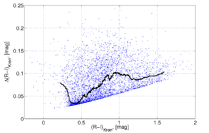
Figure 8: (R - I) colour errors as a function of (R - I) colour for $\sim$4,000 objects imaged in the same field. The black line shows a running median of errors in 200-object bins.

7 Point/Extended Source Separation

In this section we describe an empirical point/extended source separation (PES) procedure for the NCCS images. Below we refer to “extended” sources implying that they are very likely to be non-stellar, probably galaxies. The procedure is based on the SDSS star/galaxy classification.

To compare our results with the SDSS and to perform PES we obtained three 300-sec images in the R and in I filters of a field covered by the SDSS and centered on J2000.0 ($\alpha$, $\delta$) = (16^h, 40^∘) with exactly the same setup as used for the NCCS. The images were debiased, FF normalized and median-combined. After deriving the astrometric solution for the resulting images, the objects were extracted using the SE and were matched with the SDSS objects.

Our PES procedure is based on the size and shape of the sources. We defined the relative FWHM difference in R and I bands as $\epsilon$(FWHM)$=\frac{|FWHM_{R}-FWHM_{I}|}{FWHM_{R}+FWHM_{I}}$. We also defined the mean FWHM in R and I bands as $<FWHM>=\frac{FWHM_{R}+FWHM_{I}}{2}$. Fig. 9 shows plots of $\epsilon$(FWHM) vs. mean FWHM normalized by the mean seeing, for different magnitude limits. Note that the objects can be separated with reasonable accuracy using a single separation line. Different separation lines were examined using two criteria: the separation needs to match the SDSS PES as good as possible, and the mutual contaminations by point and extended sources need to be similar, i.e. with no bias to one of the classes. The first criterion implies that the number of the point/extended sources classified incorrectly by our routine relative to the SDSS should be as small as possible. The second criterion implies that the number of the point sources defined incorrectly by our routine should be similar to the number of the extended sources defined incorrectly.

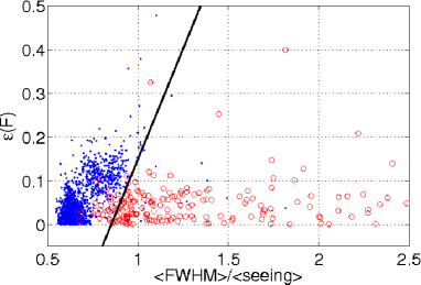
(a)		(b)
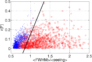
(c)

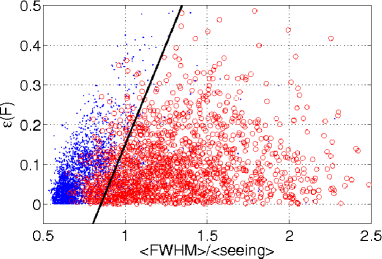
Figure 9: Relative FWHM difference $\epsilon$(FWHM) as a function of (mean FWHM)/(mean seeing). Points show objects defined by SDSS as point sources and circles show objects defined as extended by SDSS. The solid black line represents an empirical PES solution defined by equation (3). Panel (a) shows objects brighter than R$=18.6$ mag and I$=17.8$ mag. Panel (b) - objects brighter than R$=20.0$ mag and I$=19.1$ mag. Panel (c) - objects brighter than R$=20.6$ mag and I$=19.6$ mag.

The following PES solution fits best these two criteria:

$$\begin{array}[]{rcll}\epsilon(FWHM)&>&1.01\frac{<FWHM>}{<seeing>}-0.86&\rightarrow point~{}source\\ \epsilon(FWHM)&<&1.01\frac{<FWHM>}{<seeing>}-0.86&\rightarrow extended~{}source\end{array}$$ (3)

Table 6 shows the PES accuracy relative to SDSS obtained using equation (3) for different magnitude limits. The PES classification accuracy corresponding to the NCCS limiting magnitudes R${}_{lim}=20.6$ mag and I${}_{lim}=19.6$ mag, as defined in Section 6, is $\sim$91%. Since the separation requires that both the R and I band data would be available for the same object, the PES is performed following stage two of the photometric procedure. The final catalogue includes the PES flag defined for each object, which is 0 for a point source and 1 for an extended one.

Table 6: PES Accuracy Relative to the SDSS Corresponding to the Different R and I Limits:

Magnitude Limits
R	I	PES Accuracy
18.6	17.8	97.1%
20.0	19.1	93.0%
20.6	19.6	90.8%

8 Comparison with the SDSS

Here we compare the results of our observations, reductions and extraction procedures with data provided by the SDSS. Using the same SDSS field images from June 12, 2009 we compare the NCCS photometry and astrometry with the SDSS. Jordi et al. (2006) derived empirical ’global’ colour transformations between SDSS photometry and Johnson-Cousins photometric system for $\sim$4,000 standard stars. To obtain r and i band magnitudes of the NCCS objects, we use the following equations from Jordi et al. (2006):

$$\begin{array}[]{rcl}i-I&=&(0.247\pm 0.003)*(R-I)+(0.329\pm 0.002)\\ r-i&=&(1.007\pm 0.005)*(R-I)-(0.236\pm 0.003)\end{array}$$ (4)

Panels (a) and (b) in Fig. 10 show the comparison between the NCCS photometry, transformed to r and i magnitudes using equations (4), and the SDSS photometry for the objects brighter than the NCCS limiting magnitudes R${}_{lim}=20.6$ mag and I${}_{lim}=19.6$ mag, as defined in Section 6. The NCCS and SDSS photometric results correlate well; Table 7 shows the RMS deviations of the NCCS photometry relative to the SDSS photometry for different magnitude limits. Note that the RMS deviations in both bands become smaller for brighter magnitudes.

The RMS deviation values in Table 7 are greater than the RMS errors for the NCCS limiting magnitudes derived in Section 6, but are still comparable. The difference is explained by the transformation uncertainty in equations (4). The transformation uncertainty can be defined as the dispersion of the data points used to derive the transformation, which we estimate as $\sigma\sim 0.1$ mag. Therefore, the RMS deviation in the i band for the stars brighter than I$=19.6$ mag is $\sqrt{0.1^{2}+0.15^{2}}\cong 0.18$ mag, which is consistent with the value for I = 19.6 shown in Table 7. The first term under the square root sign is produced by the RMS deviation of the transformation, while the second term is produced by the RMS magnitude error of the stars with I = 19.6. The r band transformation in Jordi et al. (2006) is determined using the i band transformation, thus the transformation uncertainty $\sigma\sim 0.1$ needs to be accounted for twice. This results in a greater dispersion of the data points in the r band plot in Fig. 10 compared to that of the data points in the i band plot. The RMS deviation in the r band for stars brighter than R = 20.6 mag is $\sqrt{0.1^{2}+0.1^{2}+0.15^{2}}\cong 0.21$ mag, which is consistent with the value for R = 20.6 shown in Table 7. The RMS deviation estimations for the other magnitude limits produce the values similar to those shown in Table 7.

The shortcomings of Jordi et al. (2006) transformations were pointed out by Chonis & Gaskell (2008), who proposed their own transformations from the SDSS ugriz magnitudes to the Johnson-Cousins UBVRI magnitudes. We performed an additional check on the quality of our photometry calibration using the following equations from Chonis & Gaskell:

$$\begin{array}[]{rcl}R&=&r-(0.272\pm 0.092)*(r-i)-(0.159\pm 0.022)\\ I&=&i-(0.337\pm 0.191)*(r-i)-(0.370\pm 0.041)\end{array}$$ (5)

The comparison between the NCCS photometry and the SDSS photometry, transformed to the R and I magnitudes using equations (5), is shown in panels (c) and (d) of Fig. 10. The RMS deviations of the NCCS photometry relative to the SDSS photometry for different magnitude limits are presented in Table 7. The RMS deviation values in Table 7 are greater than the RMS errors for the NCCS limiting magnitudes derived in Section 6, but are still comparable and become smaller for brighter magnitudes. The difference is explained by the uncertainty of the transformation in equations (5) as described above. Note that the data dispersion in panels (c) and (d) of Fig. 10 is similar, since the transformation equations (5) for R and I bands are independent. Note also that there seems to be a turndown in the plots of Fig. 10 for stars with I $\gtrsim 19$, R $\gtrsim 19$ mag and $i\gtrsim 19.5$, $r\gtrsim 19.5$ mag, which can be attributed by a Malmquist bias, as explained by Chonis & Gaskell (2008).

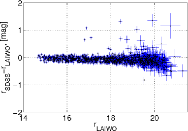
(a)		(b)
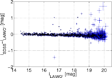
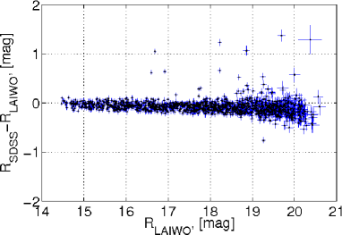
(c)		(d)

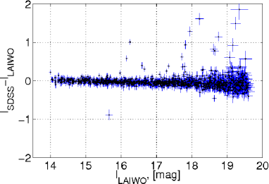
Figure 10: The NCCS photometry compared to the SDSS photometry. Panels (a) and (b) show r and i magnitudes comparison derived using the Jordi et al. (2006) transformation. Panels (c) and (d) show R and I magnitudes comparison derived using the Chonis & Gaskell (2008) transformation.

Table 7: RMS Deviations of the NCCS Photometry Relative to the SDSS Photometry Corresponding to the Different R and I Limits:

Magnitude Limits		RMS Deviation (SDSS - LAIWO)
		Jordi et al.		Chonis & Gaskell
R	I	$\sigma$(r)	$\sigma$(i)	$\sigma$(R)	$\sigma$(I)
18.6	17.8	0.17	0.10	0.16	0.09
20.0	19.1	0.20	0.14	0.18	0.14
20.6	19.6	0.21	0.17	0.19	0.17

Fig. 11 shows the comparison between the NCCS astrometry and the SDSS astrometry for the objects brighter than the NCCS limiting magnitudes R${}_{lim}=20.6$ mag and I${}_{lim}=19.6$ mag. The following RMS deviations were obtained: $\sigma(\Delta\delta)\cong 1.12$ arcsec and $\sigma(\Delta\alpha\times\cos\delta)\cong 0.83$ arcsec. These RMS deviation values are smaller than the NCCS astrometric solution RMS errors derived in Section 5.

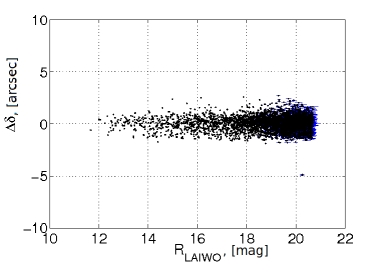
(a)		(b)
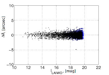
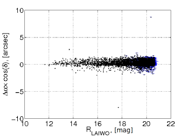
(c)		(d)

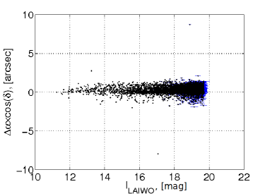
Figure 11: The NCCS astrometry compared to the SDSS astrometry. Panels (a) and (b) show the $\delta$ deviations. Panels (b) and (c) show $\alpha\times$cos($\delta$) deviations.

(a)

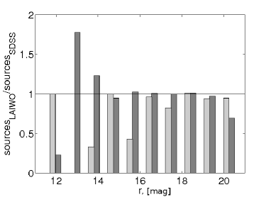
(b)

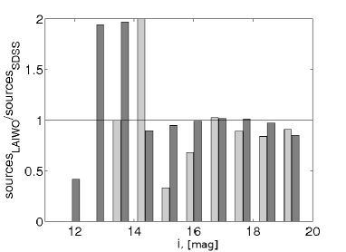
Figure 12: Number of detected souces ratio as a function of SDSS magnitude. Dark grey bars represent point sources. Light grey bars represent extended sources. Panel (a) is for the $r$ magnitude. Panel (b) is for the $i$ magnitude.

Fig. 12 shows the ratio between the number of sources detected by NCCS and the number of sources detected by SDSS in the same field, as a function of the r and i magnitudes. NCCS detects more sources brighter than $r=14.5$ and $i=14.5$ mag than the SDSS does. This is probably due to the saturation limit of the SDSS, which is $r=14.5$ and $i=14.5$ mag (Chonis & Gaskell, 2008). NCCS detects $\sim$100% of the point sources and $\sim$90% of the extended sources fainter than $r=14.5$ and $i=14.5$ mag (but brighter than the NCCS limits) detected by the SDSS in both $r$ and $i$ bands. Small deviations of the ratio from 100% are probably due to uncertainties of the photometric transformation in equation (4). Note also that the detection ratio drops for the sources fainter than $r=20$ and $i=19$ mag, which are close to the NCCS limiting R and I magnitudes defined in Section 6 and can be attributed by a Malmquist bias as explained by Chonis & Gaskell (2008)..

9 Sky Coverage and Completeness

Since February 13, 2009 we imaged 223 sky fields three times in $R$ and $I$ filters in the NCC region for a total sky coverage of $\sim$130 square degrees. Fig. 13 shows the sky coverage map in polar projection with each square representing the footprint of one of LAIWO science CCDs. The survey results will be described in a future paper.

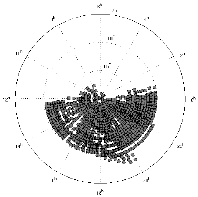
Figure 13: Sky coverage from February 13, 2009 till September 13,2009.

We use images from June 12, 2009 to estimate the catalogue completeness. Fig. 14 shows a comparison of the star count cumulative distribution with an exponential model expected for a complete catalogue. Note that no sources are missing for R $\leq 20.7$ mag and I $\leq 19.9$ mag. These completeness limits are fainter than the limiting R and I magnitudes as defined in Section 6. Therefore, we estimate that the NCCS catalogue will be complete to the limiting magnitudes as defined in Section 6.

(a)

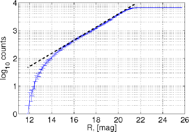
(b)

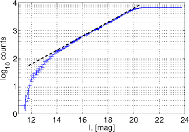
Figure 14: Star count cumulative distribution as a function of magnitude. The black dashed line shows an exponential model of a complete catalogue. The left panel is for the R magnitudes and the right panel is for the I magnitudes.

10 Multiple Detections and Variability Treatment

We expect to find multiple detections of the same source during the data reduction process. However, ‘regular’ sources should not change their brightness significantly and rapidly. Fig. 15 shows the grey magnitude RMS deviation vs. RMS grey magnitude for $\sim$2200 objects detected more than once on the images of seven fields from June 13, 2009. The median deviation for both grey magnitudes is smaller than the R and I RMS errors for the NCCS limiting magnitudes in Table 5. A particular source that changes its magnitude significantly and rapidly is recognized by our pipeline as a ‘variable’ source.

The final catalogue, after stage two of the photometry, includes two flags defined for each object. The detection flag is 1 when a particular object has been detected twice - once in R and once in I. Every new detection in R or in I band image will add one count to this flag. The variability flag is 0 for a non-variable object. Every new detection in R or in I that will return a magnitude different by $\pm 3\sigma$ of the previous detection will change the value of this flag to one, meaning that the object is potentially variable.

For the final production run the values in the catalogue will be updated following each new detection by adopting weighted means and weighted errors of the values. The values defined without errors, such as $\epsilon$(FWHM), will be updated to a simple mean.

(a)

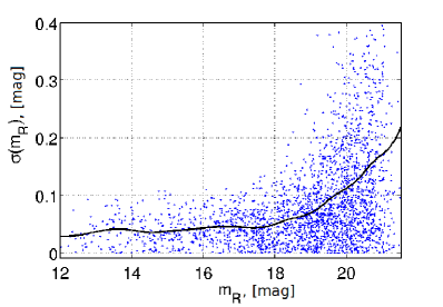
(b)

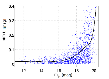
Figure 15: Grey magnitude RMS deviation vs. RMS grey magnitude for $\sim$2200 objects detected more than once. The black line shows a running median of deviation in 100 object bins. The left panel is for the m_R magnitudes and the right panel is for the m_I magnitudes.

11 Catalogue

The final catalogue after stage two of photometry includes only entries for objects detected at least once in R and once in I. The final catalogue does not contain objects defined as truncated by the NCCS pipeline or those with SE internal flag $>$3. This implies that only objects defined as ‘regular’, or deblended objects, or objects restored from the 10% overlaping with another object, are included in the final catalogue. The final catalogue contains the parameters listed in Table 8 and an example of a page from the final catalogue is shown in Table 9.

Table 8: Output Parameters of Final Catalogue:

#	Catalog Parameter	Units
1	J2000.0 $\alpha$	hh:mm:ss
2	$\Delta\alpha$	sec
3	J2000.0 $\delta$	dd:mm:ss
4	$\Delta\delta$	arcsec
5	Kron R flux	ADU/sec
6	Kron R flux error	ADU/sec
7	Kron I flux	ADU/sec
8	Kron I flux error	ADU/sec
9	Kron R magnitude	mag
10	Kron R magnitude error	mag
11	Kron I magnitude	mag
12	Kron I magnitude error	mag
13	FWHMR	pix
14	FWHMI	pix
15	$a_{R}$	pix
16	$b_{R}$	pix
17	$\theta_{R}$	deg
18	$a_{I}$	pix
19	$b_{I}$	pix
20	$\theta_{I}$	deg
21	$\epsilon$(FWHM)	unitless
22	$<$FWHM$>$/$<$seeing$>$	unitless
23	Point/extended source	unitless
24	Detection number	unitless
25	Variability flag	unitless

12 Conclusions

We described procedures, data treatment, and expected photometric and astronomic accuracies of a survey of the NCC performed at the Wise Observatory in the R and I bands with the LAIWO CCD mosaic on the Wise Observatory’s one meter telescope. The survey detects some 4,000 sources per square degree. The source catalog lists their ($\alpha,\delta$) coordinates to $\lesssim 1^{\prime\prime}$ and their R and I magnitudes accurate to 0.15 mag or better for sources brighter than 20.6 in R or 19.6 in I. Essentially $>$90% of the objects classified by SDSS as point/galactic sources are recognized as such by our survey. The survey results will be used in conjunction with the data from the TAUVEX UV space telescope to characterize the UV sources.

13 Acknowledgements

LAIWO has been built at the Max-Planck-Institute for Astronomy (MPIA) in Heidelberg, Germany with the financial support from MPIA, and grants from the German-Israel Foundation and from the Israel Science Foundation as a scientific collaboration between Tel Aviv University and MPIA. We are grateful to our German colleagues for constructing this instrument and to Dr. Shai Kaspi, the LAIWO liaison scientist at Tel Aviv University. We acknowledge the considerable technical help tended by the Wise Observatiry staff, Mr. Ezra Mashal and Mr. Sammy Ben Guigui, and MPIA Heidelberg Dr. Karl-Heinz Marien, the project manager, Mr. Ralf Klein, Mr. Florian Briegel, and Mr. Harald Baumeister.

Funding for the Sloan Digital Sky Survey (SDSS) has been provided by the Alfred P. Sloan Foundation, the Participating Institutions, the National Aeronautics and Space Administration, the National Science Foundation, the U.S. Department of Energy, the Japanese Monbukagakusho, and the Max Planck Society. The SDSS Web site is http://www.sdss.org/.

The SDSS is managed by the Astrophysical Research Consortium (ARC) for the Participating Institutions. The Participating Institutions are The University of Chicago, Fermilab, the Institute for Advanced Study, the Japan Participation Group, The Johns Hopkins University, Los Alamos National Laboratory, the Max-Planck-Institute for Astronomy (MPIA), the Max-Planck-Institute for Astrophysics (MPA), New Mexico State University, University of Pittsburgh, Princeton University, the United States Naval Observatory, and the University of Washington.

Table 9: Final Catalogue Example:

References

- Abazajian et al. (2009) Abazajian, K. N., et al. 2009, Astrophysical Journal Supplement Series, 182, 543
-
Afonso (2007)
Afonso C., The Large Area Imager for the Wise Observatory, LAIWO,
User Manual, 2007,
http://www.mpia.de/transits/minerva/Laiwo/LAIWOUserManual.html - Baumeister et al. (2006) Baumeister, H., Afonso, C., Marien, K.-H., & Klein, R. 2006, Proceedings of the SPIE, 6269,
- Bertin & Arnouts (1996) Bertin, E., & Arnouts, S. 1996, A&AS, 117, 393
- Chonis & Gaskell (2008) Chonis, T. S., & Gaskell, C. M. 2008, AJ, 135, 264
- Cousins (1974) Cousins, A. W. J. 1974, Monthly Notes of the Astronomical Society of South Africa, 33, 149
- Graham & Driver (2005) Graham, A. W., & Driver, S. P. 2005, Publications of the Astronomical Society of Australia, 22, 118
- Hanisch et al. (2001) Hanisch, R. J., Farris, A., Greisen, E. W., Pence, W. D., Schlesinger, B. M., Teuben, P. J., Thompson, R. W., & Warnock, A., III 2001, A&A, 376, 359
- Johnson & Morgan (1953) Johnson, H. L., & Morgan, W. W. 1953, ApJ, 117, 313
- Jordi et al. (2006) Jordi, K., Grebel, E. K., & Ammon, K. 2006, A&A, 460, 339
-
Kaspi (2009)
Kaspi, S., Manuals for the Wise Observatory, 2009,
http://wise-obs.tau.ac.il/observations/Man/ - Kron (1980) Kron, R. G. 1980, Astrophysical Journal Supplement Series, 43, 305
- Landolt (2009) Landolt, A. U. 2009, AJ, 137, 4186
- Mink (2002) Mink, D. J. 2002, Astronomical Data Analysis Software and Systems XI, 281, 169
- Monet (1998) Monet, D. G. 1998, Bulletin of the American Astronomical Society, 30, 1427
- Monet et al. (2003) Monet, D. G., et al. 2003, AJ, 125, 984
- Nelder & Mead (1965) Nelder, J.A., & Mead, R. 1965, A simplex method for function minimization. Computer Journal, 7:308–313
- Reshetnikov (2005) Reshetnikov, V. P. 2005, Physics Uspekhi, 48, 1109
- Skrutskie et al. (2006) Skrutskie, M. F., et al. 2006, AJ, 131, 1163
- Tody (1986) Tody, D. 1986, Proceedings of the SPIE, 627, 733