On a possible approach to general field theories with nonpolynomial interactions

Abstract

In this work a class of field theories with self-interactions described by a potential of the kind $V(\phi(x)-\phi(x_{0}))$ is studied. $\phi$ is a massive scalar field and $x,x_{0}$ are points in a $d$ dimensional space. Under the condition that the potential admits the Fourier representation, it is shown that such theories may be mapped into a standard field theory, in which the interaction of the new fields is a polynomial of fourth degree. With some restrictions, this mapping allows the perturbative treatment of models that are otherwise intractable with standard field theoretical methods.

A nonperturbative approach to these theories is attempted. The original scalar field $\phi$ is integrated out exactly at the price of introducing auxiliary vector fields. The latter are treated in a mean field theory approximation. The singularities that arise after the elimination of the auxiliary fields are cured using the dimensional regularization. The expression of the counterterms to be subtracted is computed.

I Introduction

In this letter we study a wide class of $d-$dimensional field theories in which the interactions are described by a general potential $V(\phi(x)-\phi(x_{0}))$. Here $\phi(x)$, $x\in\mathbb{R}^{d}$ denotes a massive scalar field. $x_{0}$ is a fixed point in $\mathbb{R}^{d}$. The only requirement on the potential $V$ is that its Fourier representation exists, i. e. it is possible to write $V(\phi)=\int_{-\infty}^{+\infty}db\tilde{V}(b)e^{-ib\phi}$. It is shown that all theories of this kind can be mapped into a $(d+2)-$dimensional field theory, in which the interactions between the fields are polynomial. As a consequence, models which are highly nonlinear and nonlocal may be treated after the mapping using perturbative methods. This is the main result of this work. The mapping is obtained extending a technique known in statistical mechanics as Gaussian integration gi1 ; gi2 ; gi2 ; gi4 ; gi5 , which allows to identify certain field theories with a gas of interacting particles. In the present case a field theory is identified with another field theory. Yet, Gaussian integration is used at some step in order to simplify the interaction term of the original massive scalar fields. More precisely, the term $e^{-V}$ is rewritten in the form of the “equilibrium limit” of the partition function of a system of quantum particles interacting with the field $\phi$. A similar strategy has been recently applied in FePa to reformulate the Liouville field theory as a theory with polynomial interactions, which is very similar to scalar electrodynamics. A brief introduction to the method and a discussion of its advantages can be found in Ref. FePa2 . As a result of the whole procedure, we obtain a theory of complex scalar fields $\psi^{*},\psi$ describing the fluctuations of particles immersed in the purely longitudinal vector potential $\mathbf{A}=\nabla\phi$.

In the second part of this letter, a nonperturbative approach is attempted. First of all, the field $\phi$ is integrated out using a technique similar to that exploited in the case of Chern-Simons fields in Ref. Femultifield . In this way a set of new vector fields $\bm{\xi}^{*},\bm{\xi}$ is introduced, which are treated using a mean field theory approximation. The arising singularities are computed with the help of the dimensional regularization. This does not exhaust all possible divergences that may arise in the theory. A discussion of renormalization issues is presented in the Conclusions.

II The Mapping

We consider here the class of $d-$dimensional field theories with partition function

$$Z=\int{\cal D}\phi e^{-S}$$ (1)

and action

$$S=\int d^{d}x\left[\frac{1}{2}(\nabla\phi)^{2}+\frac{m^{2}}{2}\phi^{2}+V(\phi(x)-\phi(x_{0}))\right]$$ (2)

The potential $V(\phi(x)-\phi(x_{0}))$ is given in the Fourier representation:

$$V(\phi(x)-\phi(x_{0}))=\int_{-\infty}^{+\infty}db\tilde{V}(b)e^{-ib(\phi(x)-\phi(x_{0}))}$$ (3)

One can obtain in this way a wide class of potentials. For example, the potential:

$$V_{1}(\phi(x)-\phi(x_{0}))=\frac{k_{1}}{a^{2}+(\phi(x)-\phi(x_{0}))^{2}}$$ (4)

corresponds to the choice $\tilde{V}(b)=\frac{k_{1}}{2a}e^{-a|b|}$ with $a>0$.

Putting instead $\tilde{V}_{2}(b)=\frac{k_{2}}{\sqrt{4a\pi}}\sin\left(\frac{b^{2}}{4a}+\frac{\pi}{4}\right)$ we have

$$V_{2}(\phi(x)-\phi(x_{0}))=k_{2}\sin\left(a(\phi(x)-\phi(x_{0}))^{2}\right)$$ (5)

Potentials of this kind, which contain in general infinite powers of the fields as Eqs. (4) and (5) show, can be simplified with the help of the following identity:

$$\exp\left[\int_{-\infty}^{+\infty}db\tilde{V}(b)e^{-ib(\phi(x)-\phi(x_{0}))}\right]=\lim_{T\to+\infty}\Xi_{T}[\phi]$$ (6)

where

$$\Xi_{T}[\phi]=\int{\cal D}\psi^{*}{\cal D}\psi\exp\left\{-i\int dbdtd^{d}x\left[i\psi^{*}\frac{\partial\psi}{\partial t}-g|(\nabla+ib\nabla\phi)\psi|^{2}-J^{*}\psi-J\psi^{*}\right]\right\}$$ (7)

while $\psi=\psi(t,x,b)$ and $\psi^{*}=\psi^{*}(t,x,b)$. In Eq. (7) the currents $J^{*},J$ have been chosen as follows:

$$J^{*}(t)=(4\pi igT)^{\frac{d}{2}}\delta(t)\qquad\qquad J(t,x,b)=-\delta(x-x_{0})\tilde{V}(b)\delta(t-T)$$ (8)

Let us prove the above identity. The complex field $\psi^{*}$ in Eq. (7) is a Lagrange multiplier that imposes the condition:

$$i\frac{\partial\psi}{\partial t}+g(\nabla+ib\nabla\phi)^{2}\psi=J$$ (9)

The solution of this equation is:

$$\psi(t,x,b)=\int db^{\prime}dt^{\prime}d^{d}x^{\prime}{\cal G}(t-t^{\prime},x-x^{\prime},b-b^{\prime})J(t^{\prime},x^{\prime},b^{\prime})$$ (10)

where

$${\cal G}(t-t^{\prime},x-x^{\prime},b-b^{\prime})=-\frac{i\theta(t-t^{\prime})}{|4\pi ig(t-t^{\prime})|^{\frac{d}{2}}}\exp\left[i\frac{(x-x^{\prime})^{2}}{4g(t-t^{\prime})}\right]e^{-ib\phi(x)}e^{ib^{\prime}\phi(x^{\prime})}\delta{(b-b^{\prime})}$$ (11)

and $\theta(t-t^{\prime})$ is the Heaviside function. As a consequence, it is not difficult after integrating out the fields $\psi^{*}$ and $\psi$ to show that

$$\Xi_{T}[\phi]=\exp\left\{+\int dbdtd^{d}xdt^{\prime}dx^{\prime}J^{*}(t,x){\cal G}_{0}(t-t^{\prime},x-x^{\prime})e^{-ib\phi(x)}e^{ib\phi(x^{\prime})}J(t,x,b)\right\}$$ (12)

In the above equation we have put for convenience:

$${\cal G}_{0}(t-t^{\prime},x-x^{\prime})=-\frac{i\theta(t-t^{\prime})}{|4\pi ig(t-t^{\prime})|^{\frac{d}{2}}}\exp\left[i\frac{(x-x^{\prime})^{2}}{4g(t-t^{\prime})}\right]$$ (13)

Let us note that in principle the right hand side of Eq. (12) should be multiplied by the determinant of the operator $A^{-1}$, where

$$A=i\frac{\partial}{\partial t}+g(\nabla+ib\nabla\phi)^{2}$$ (14)

However, it will be proved in the Appendix that $\det(A^{-1})=1$. The reason, as explained in gi5 , is that in non-relativistic theories like those treated here, there are no antiparticles and therefore charged loops vanish identically. An explicit verification that indeed $\det(A^{-1})$ is trivial in theories in which the propagator is proportional to $\theta(t-t^{\prime})$ can be performed following the procedure of Ref. FePa .

Substituting in Eq. (12) the expressions of the currents $J^{*},J$ given in Eq. (8), we obtain:

$$\Xi_{T}[\phi]=\exp\left\{-\int dbd^{d}x\tilde{V}(b)e^{-ib({\phi(x)-\phi(x_{0})})}e^{i\frac{(x-x_{0})^{2}}{4gT}}\right\}$$ (15)

In the limit $T\longrightarrow+\infty$ the generating functional $\Xi_{T}[\phi]$ of the fields $\psi^{*},\psi$ together with the special choice of currents (8) coincides exactly with the left hand side of Eq. (6).

In conclusion, it has been shown that the partition function of the nonlinear and nonlocal scalar field theory given in Eqs. (1) and (2) can be rewritten in the form of the equilibrium limit of a local field theory:

$$Z=\lim_{T\longrightarrow+\infty}\int{\cal D}\phi e^{-\int d^{d}x\left(\frac{1}{2}(\nabla\phi)^{2}+\frac{m^{2}}{2}\phi^{2}\right)}\Xi_{T}[\phi]$$ (16)

III Non-perturbative approach

Let us write Eq. (16) explicitly:

$$Z = \lim_{T\to+\infty}\int{\cal D}\phi{\cal D}\psi^{*}{\cal D}\psi\exp\left\{-\int d^{d}x\left(\frac{1}{2}(\nabla\phi)^{2}+\frac{m^{2}}{2}\phi^{2}\right)\right\}$$ (17)

$$\times \exp\left\{-i\int dbdtd^{d}x\left[i\psi^{*}\frac{\partial\psi}{\partial t}-g|(\nabla+ib\nabla\phi)\psi|^{2}-J^{*}\psi-J\psi^{*}\right]\right\}$$

In order to eliminate the field $\phi$, we introduce following Femultifield the complex vector fields $\bm{\xi}^{*},\bm{\xi}$ and express $Z$ as follows:

$$Z = \lim_{T\longrightarrow+\infty}\int{\cal D}\phi{\cal D}\psi^{*}{\cal D}\psi{\cal D}\bm{\xi}^{*}{\cal D}\bm{\xi}\exp\left\{-\int d^{d}x\left[\frac{1}{2}(\nabla\phi)^{2}+\frac{m^{2}}{2}\phi^{2}\right]\right\}$$ (18)

$$\times \exp\left\{-i\int dbdtd^{d}x\left[i\psi^{*}\frac{\partial\psi}{\partial t}+g\bm{\xi}^{*}\cdot\bm{\xi}-g\bm{\xi}^{*}\cdot(\nabla+ib\nabla\phi)\psi\right.\right.$$

$$\left.\left.\phantom{\frac{\partial\psi}{\partial t}}-g(\nabla-ib\nabla\phi)\psi^{*}\cdot\bm{\xi}-J^{*}\psi-J\psi^{*}\right]\right\}$$

It is easy to check that Eq. (17) is recovered after eliminating the fields $\bm{\xi}^{*},\bm{\xi}$ from Eq. (18). At this point we isolate in the expression of $Z$ the contribution due to the field $\phi$:

$$Z = \lim_{T\to+\infty}\int{\cal D}\psi^{*}{\cal D}\psi{\cal D}\bm{\xi}^{*}{\cal D}\bm{\xi}\exp\left\{-i\int dbdtd^{d}x\left[i\psi^{*}\frac{\partial\psi}{\partial t}+\right.\right.$$ (19)

$$+ \left.\left.\!\!\!\!\!\!\!\!\!\!\!\!\!\!\phantom{*\frac{\partial\psi}{\partial t}}g\bm{\xi}^{*}\cdot\bm{\xi}-g\bm{\xi}^{*}\cdot\nabla\psi-g\bm{\xi}\cdot\nabla\psi^{*}-\psi J^{*}-\psi^{*}J\right]\right\}Z_{\phi}$$

where

$$Z_{\phi}=\int{\cal D}\phi e^{-\int d^{d}x\left[\frac{1}{2}(\nabla\phi)^{2}+\frac{m^{2}}{2}\phi^{2}-g\phi\nabla\cdot\int dbdtb\left(\bm{\xi}^{*}\psi-\bm{\xi}\psi^{*}\right)\right]}$$ (20)

$Z_{\phi}$ is the partition function of a free scalar field theory in the presence of the external current:

$$K(x)=\nabla\cdot\int dbdtb\left(\bm{\xi}^{*}\psi-\bm{\xi}\psi^{*}\right)$$ (21)

Let us note that this current is purely imaginary. After performing the simple gaussian integration over $\phi$ we obtain:

$$Z_{\phi}=\exp\left\{\frac{g^{2}}{2}\int d^{d}xd^{d}x^{\prime}G(x,x^{\prime})K(x)K(x^{\prime})\right\}$$ (22)

$G(x,x^{\prime})$ denotes the scalar field propagator:

$$G(x,x^{\prime})=\int\frac{d^{d}p}{(2\pi)^{d}}\frac{e^{-ip\cdot(x-x^{\prime})}}{p^{2}+m^{2}}$$ (23)

The total sign of the exponent appearing in the right hand side of Eq. (22) is negative. To show that, we put $G(x,x^{\prime})=\sum_{n=0}^{+\infty}\frac{\phi_{n}(x)\phi_{n}(x^{\prime})}{\lambda_{n}}$, where the $\phi_{n}(x)$’s are the eigenfunctions of the $d-$dimensional differential operator $\Delta-m^{2}$ and the $\lambda_{n}$’s are their respective eigenvalues. Thus Eq. (22) may be rewritten as follows:

$$Z_{\phi}=\exp\left\{\frac{g^{2}}{2}\sum_{n=0}^{+\infty}\frac{1}{\lambda_{n}}\left[\int d^{d}x\phi_{n}(x)K(x)\right]^{2}\right\}$$ (24)

Due to the fact that the eigenvalues $\lambda_{n}$ are positive and $K(x)$ is purely imaginary, the total sign of the exponent in the above equation is negative as desired.

At this point it will be convenient to introduce the following shorthand notation: $\eta=x,b,t$ and $d^{d+2}\eta=d^{d}xdbdt$, so that

$$Z_{\phi}=e^{\left\{\frac{g^{2}}{2}\int d^{d+2}\eta d^{d+2}\eta^{\prime}\big{[}bb^{\prime}G_{\mu\nu}(x,x^{\prime})\big{(}\xi^{*\mu}(\eta)\psi(\eta)-\xi^{\mu}(\eta)\psi^{*}(\eta)\big{)}\big{(}\xi^{*\nu}(\eta^{\prime})\psi(\eta^{\prime})-\xi^{\nu}(\eta^{\prime})\psi^{*}(\eta^{\prime})\big{)}\big{]}\right\}}$$ (25)

where

$$G_{\mu\nu}(x,x^{\prime})=-\int\frac{d^{d}p}{(2\pi)^{d}}{e^{-ip\cdot(x-x^{\prime})}}\frac{p_{\mu}p_{\nu}}{p^{2}+m^{2}}\qquad\qquad\mu,\nu=1,\ldots,d$$ (26)

In writing Eq. (22) we have used the explicit form of the current $K(x)$ given in Eq. (21) and some integrations by parts. Substituting the expression of $Z_{\phi}$ of Eq. (25) back in the original Eq. (19), the total partition function $Z$ becomes:

$$Z=\lim_{T\to+\infty}\int{\cal D}\psi^{*}{\cal D}\psi{\cal D}\bm{\xi}^{*}{\cal D}\bm{\xi}e^{-iS_{0}+S_{int}}$$ (27)

where

$$S_{0}=\int d^{d+2}\eta\left[i\psi^{*}\frac{\partial\psi}{\partial t}+g\bm{\xi}^{*}\cdot\bm{\xi}-g\bm{\xi}^{*}\cdot\nabla\psi-g\bm{\xi}\cdot\nabla\psi^{*}-\psi J^{*}-\psi^{*}J\right]$$ (28)

is the free part of the action, while the interaction term is:

$$S_{int}=\frac{g^{2}}{2}\int d^{d+2}\eta d^{d+2}\eta^{\prime}\big{[}bb^{\prime}G_{\mu\nu}(x,x^{\prime})\big{(}\xi^{*\mu}(\eta)\psi(\eta)-\xi^{\mu}(\eta)\psi^{*}(\eta)\big{)}\big{(}\xi^{*\nu}(\eta^{\prime})\psi(\eta^{\prime})-\xi^{\nu}(\eta^{\prime})\psi^{*}(\eta^{\prime})\big{)}\big{]}$$ (29)

This is the effective interaction resulting from the integration over the fields $\phi$. Indeed, it is easy to realize that $S_{int}$ coincides with the exponent of $Z_{\phi}$ in Eq. (25). The fact that this exponent is always negative assures the convergence of the further integrations over the remaining fields.

In the free action $S_{0}$ of Eq. (28) the fields $\bm{\xi}^{*},\bm{\xi}$ and $\psi^{*},\psi$ are coupled together. To disentangle this unwanted coupling, we perform the following shift of variables:

$$\bm{\xi}^{*}=\nabla\psi^{*}+\delta\bm{\xi}^{*}\qquad\qquad\bm{\xi}=\nabla\psi+\delta\bm{\xi}$$ (30)

The new fields $\delta\bm{\xi}^{*},\delta\bm{\xi}$ may be interpreted as the fluctuations of the fields $\bm{\xi}^{*},\bm{\xi}$ around their classical configurations that are respectively given by $\nabla\psi^{*}$ and $\nabla\psi$.

Applying the shift (30) to Eq. (27) we obtain:

$$Z=\lim_{T\to+\infty}\int{\cal D}\psi^{*}\int{\cal D}\psi\int{\cal D}(\delta\bm{\xi}^{*})\int{\cal D}(\delta\bm{\xi})e^{-iS_{0,\delta}+S_{int,\delta}}$$ (31)

Now the free action $S_{0,\delta}$ does not contain unwanted interactions between the fields $\psi^{*},\psi$ and the new fields $\delta\bm{\xi}^{*},\delta\bm{\xi}$:

$$S_{0,\delta}=\int d^{d+2}\eta\left[i\psi^{*}\frac{\partial\psi}{\partial t}-g\nabla\psi^{*}\cdot\nabla\psi+g\delta\bm{\xi}^{*}\cdot\delta\bm{\xi}-\psi J^{*}-\psi^{*}J\right]$$ (32)

The nonlinear part $S_{int,\delta}$ is given by:

$$S_{int,\delta} = \frac{g^{2}}{2}\int d^{d+2}\eta d^{d+2}\eta^{\prime}\Big{[}bb^{\prime}G_{\mu\nu}(x,x^{\prime})\Big{(}\partial^{\mu}\psi^{*}(\eta)\partial^{\nu}\psi^{*}(\eta^{\prime})\psi(\eta)\psi(\eta^{\prime})+$$ (33)

$$+ \partial^{\mu}\psi(\eta)\partial^{\nu}\psi(\eta^{\prime})\psi^{*}(\eta)\psi^{*}(\eta^{\prime})-2\partial^{\mu}\psi^{*}(\eta)\partial^{\nu}\psi(\eta^{\prime})\psi(\eta)\psi^{*}(\eta^{\prime})+$$

$$+ 2\partial^{\mu}\psi^{*}(\eta)\delta\xi^{*\nu}(\eta^{\prime})\psi(\eta)\psi(\eta^{\prime})-2\partial^{\mu}\psi^{*}(\eta)\delta\xi^{\nu}(\eta^{\prime})\psi(\eta)\psi^{*}(\eta^{\prime})-$$

$$- \delta\xi^{*\mu}(\eta^{\prime})\partial^{\nu}\psi(\eta)\psi(\eta)\psi^{*}(\eta^{\prime})+2\partial^{\mu}\psi(\eta)\delta\xi^{\nu}(\eta^{\prime})\psi^{*}(\eta)\psi^{*}(\eta^{\prime})+$$

$$+ \delta\xi^{*\mu}(\eta)\delta\xi^{\nu}(\eta^{\prime})\psi(\eta)\psi(\eta^{\prime})+\delta\xi^{\mu}(\eta)\delta\xi^{\nu}(\eta^{\prime})\psi^{*}(\eta)\psi^{*}(\eta^{\prime})-$$

$$- 2\delta\xi^{*\mu}(\eta)\delta\xi^{\nu}(\eta^{\prime})\psi(\eta)\psi^{*}(\eta^{\prime})\Big{)}\Big{]}$$

where $\partial^{\mu}=\frac{\partial}{\partial x_{\mu}}$. At this point we can expand the partition function $Z$ in powers of the currents $J$ and $J^{*}$:

$$Z = \lim_{T\to+\infty}\sum_{n=1}^{\infty}\sum_{m=1}^{\infty}\int d^{d+2}\eta_{1}\cdots\int d^{d+2}\eta_{n}\int d^{d+2}\eta_{1}^{\prime}\cdots\int d^{d+2}\eta_{m}\times$$ (34)

$$\times Z^{(nm)}(\eta_{1},\ldots,\eta_{n};\eta_{1}^{\prime},\ldots,\eta_{m}^{\prime})J(\eta_{1})\cdots J(\eta_{n})J^{*}(\eta_{1})\cdots J^{*}(\eta_{n})$$

It is easy to check that in the above series many terms disappear in the limit $T\longrightarrow+\infty$. They vanish due to the effect of the propagators of the fields $\psi^{*},\psi$ that are given by Eq. (13). In Eq. (34), due to the special form of the currents $J^{*},J$ defined in Eq. (8), these propagators have to be evaluated in the special case $t-t^{\prime}=T$. As a consequence, each contraction of the fields $\psi^{*},\psi$ generates a factor $T^{-\frac{d}{2}}$ and, for this reason, many Feynman diagrams are suppressed in the limit $T\longrightarrow+\infty$. Only those terms in which the factors $T^{-\frac{d}{2}}$ are exactly compensated by the positive powers of $T$ contained in the currents $J^{*}$ survive.

It is also possible to show that the partition function (31) is independent of the value of the coupling constant appearing in the actions $S_{0,\delta}$ and $S_{int,d}$ of Eqs. (32)–(33) respectively. This could be expected from the fact that the parameter $g$ does not appear in the original model of Eqs. (1)–(2). To prove that, we consider the path integral $Z_{g}(T)$ in the left hand side of Eq. (31) before taking the limit $T\longrightarrow+\infty$. Clearly $Z=\lim_{T\to+\infty}Z_{g}(T)=Z_{g}(+\infty)$. Analogously, we will use the symbols $S_{0,\delta}(g,T)$ and $S_{int,\delta}(g)$ for the actions $S_{0,\delta}$ and $S_{int,\delta}$ in order to emphasize their dependence on the parameters $g$ and $T$. It will be shown in the following that

$$Z_{g}(+\infty)=Z_{g^{\prime}}(+\infty)$$ (35)

even if $g$ and $g^{\prime}$ do not coincide. To begin with, we perform in the free action $S_{0,\delta}(g,T)$ and in the interation part $S_{int,\delta}(g)$ the time rescaling:

$$t=\frac{g^{\prime}}{g}t^{\prime}$$ (36)

After the above rescaling, $S_{0,\delta}(g,T)$ and $S_{int,\delta}(g)$ read as follows:

$$S_{0,\delta}(g^{\prime},\frac{g}{g^{\prime}}T)=\int dt^{\prime}dbd^{d}x\left[i\psi^{*}\frac{\partial\psi}{\partial t}-g^{\prime}\nabla\psi^{*}\cdot\nabla\psi+g^{\prime}\delta\bm{\xi}^{*}\cdot\delta\bm{\xi}-\frac{g^{\prime}}{g}\psi J^{*}-\frac{g^{\prime}}{g}\psi^{*}J\right]$$ (37)

and

$$S_{int,\delta}(g^{\prime}) = \frac{{g^{\prime}}^{2}}{2}\int d^{d}xdbdtd^{d}x^{\prime}db^{\prime}dt^{\prime}\Big{[}bb^{\prime}G_{\mu\nu}(x,x^{\prime})\Big{(}\partial^{\mu}\psi^{*}(\eta)\partial^{\nu}\psi^{*}(\eta^{\prime})\psi(\eta)\psi(\eta^{\prime})+$$ (38)

$$+ \partial^{\mu}\psi(\eta)\partial^{\nu}\psi(\eta^{\prime})\psi^{*}(\eta)\psi^{*}(\eta^{\prime})-2\partial^{\mu}\psi^{*}(\eta)\partial^{\nu}\psi(\eta^{\prime})\psi(\eta)\psi^{*}(\eta^{\prime})+$$

$$+ 2\partial^{\mu}\psi^{*}(\eta)\delta\xi^{*\nu}(\eta^{\prime})\psi(\eta)\psi(\eta^{\prime})-2\partial^{\mu}\psi^{*}(\eta)\delta\xi^{\nu}(\eta^{\prime})\psi(\eta)\psi^{*}(\eta^{\prime})-$$

$$- \delta\xi^{*\mu}(\eta^{\prime})\partial^{\nu}\psi(\eta)\psi(\eta)\psi^{*}(\eta^{\prime})+2\partial^{\mu}\psi(\eta)\delta\xi^{\nu}(\eta^{\prime})\psi^{*}(\eta)\psi^{*}(\eta^{\prime})+$$

$$+ \delta\xi^{*\mu}(\eta)\delta\xi^{\nu}(\eta^{\prime})\psi(\eta)\psi(\eta^{\prime})+\delta\xi^{\mu}(\eta)\delta\xi^{\nu}(\eta^{\prime})\psi^{*}(\eta)\psi^{*}(\eta^{\prime})-$$

$$- 2\delta\xi^{*\mu}(\eta)\delta\xi^{\nu}(\eta^{\prime})\psi(\eta)\psi^{*}(\eta^{\prime})\Big{)}\Big{]}$$

We remark that in the above equation $t$ and $t^{\prime}$ denote the new time variable obtained after the rescaling of Eq. (36). Moreover, the fields depend on the time $t^{\prime}$ multiplied by the scaling factor $\frac{g^{\prime}}{g}$, i. e. $\eta=\frac{g^{\prime}}{g}t,x,b$ and $\eta^{\prime}=\frac{g^{\prime}}{g}t^{\prime},x,b$. Apart from this implicit dependence, the parameter $g$ appears also explicitly in the current term of the free action of Eq. (37). There is no other dependence on $g$ both in the free action and in the interaction term of Eq. (38).

It turns out that the presence of $g$ in the current term is limited to a factor $\frac{g}{g^{\prime}}$ which rescales the time $T$. To show that, we write down the expression of this current term, which, apart from an irrelevant overall constant, is equal to:

$$S_{curr,\delta}(g^{\prime},\frac{g}{g^{\prime}}T) = \int dbdt^{\prime}d^{d}x\frac{g^{\prime}}{g}\left[\left(4\pi ig^{\prime}\left(\frac{g}{g^{\prime}}T\right)\right)^{\frac{d}{2}}\delta\left(\frac{g^{\prime}}{g}t^{\prime}\right)\psi(\frac{g^{\prime}}{g}t^{\prime},x,b)+\right.$$ (39)

$$+ \left.\delta^{(d)}(x-x_{0}){\tilde{V}}(b)\delta\left(\frac{g^{\prime}}{g}t^{\prime}-T\right)\psi^{*}(\frac{g^{\prime}}{g}t,x,b)\right]$$

Using the following identities between dirac delta functions

$$\delta(\frac{g^{\prime}}{g}t^{\prime})=\frac{g}{g^{\prime}}\delta(t^{\prime})\qquad\qquad\delta\left(\frac{g^{\prime}}{g}t^{\prime}-T\right)=\frac{g}{g^{\prime}}\delta\left(t^{\prime}-\frac{g}{g^{\prime}}T\right)$$ (40)

the expression of $S_{curr}(g^{\prime},\frac{g}{g^{\prime}}T)$ becomes:

$$S_{curr,\delta}(g^{\prime},\frac{g}{g^{\prime}}T) = \int dbdt^{\prime}d^{d}x\left[\left(4\pi ig^{\prime}\left(\frac{g}{g^{\prime}}T\right)\right)^{\frac{d}{2}}\delta(t^{\prime})\psi(\frac{g^{\prime}}{g}t^{\prime},x,b)+\right.$$ (41)

$$+ \left.\delta^{(d)}(x-x_{0}){\tilde{V}}(b)\delta\left(t^{\prime}-\frac{g}{g^{\prime}}T\right)\psi^{*}(\frac{g^{\prime}}{g}t,x,b)\right]$$

It is clear from the above equation that, as predicted, the old coupling constant $g$ enters in current term $S_{curr,\delta}(g^{\prime},\frac{g}{g^{\prime}}T)$ only inside the scaling factor $\frac{g}{g^{\prime}}$ of the time $T$. There is no other explicit dependence on $g$ in the action. In fact, if we put $J=J^{*}=0$ it is easy to realize that the old coupling constant $g$ has been already replaced by $g^{\prime}$ in the free action of Eq. (37) and in the interaction term of Eq. (38).

Of course we have to remember that, after the time rescaling of Eq. (36), $g$ is still appearing inside the fields, because their dependence on the time variable is of the form $\psi^{*}=\psi^{*}(\frac{g^{\prime}}{g}t^{\prime},x,b)$ and $\psi=\psi(\frac{g^{\prime}}{g}t^{\prime},x,b)$. Analogous equations are valid for $\delta\bm{\xi}^{*}$ and $\delta\bm{\xi}$. However, since we have to perform a path integration over all field configurations, this implicit presence of $g$ may be easily eliminated inside the path integral by the change of variables:

$$\psi^{*\prime}(t^{\prime},x,b)=\psi(\frac{g^{\prime}}{g}t^{\prime},x,b) \psi^{*\prime}(t^{\prime},x,b)=\psi(\frac{g^{\prime}}{g}t^{\prime},x,b)$$ (42)

$$\bm{\xi}^{*\prime}(t^{\prime},x,b)=\bm{\xi}(\frac{g^{\prime}}{g}t^{\prime},x,b) \bm{\xi}^{*\prime}(t^{\prime},x,b)=\bm{\xi}(\frac{g^{\prime}}{g}t^{\prime},x,b)$$ (43)

Summarizing, we are able to write the following identity:

$$Z_{g}(T)=Z_{g^{\prime}}(\frac{g}{g^{\prime}}T)$$ (44)

where

$$Z_{g^{\prime}}(\frac{g}{g^{\prime}}T)=\int{\cal D}\psi^{*\prime}\int{\cal D}\psi^{\prime}\int{\cal D}(\delta\bm{\xi}^{*\prime})\int{\cal D}(\delta\bm{\xi}^{\prime})e^{-iS_{0,\delta}(g^{\prime},\frac{g}{g^{\prime}}T)+S_{int,\delta}(g^{\prime})}$$ (45)

The actions $S_{0,\delta}(g^{\prime},\frac{g}{g^{\prime}}T)$ and $S_{int,\delta}(g^{\prime})$ in Eq. (45) are given by:

$$S_{0,\delta}(g^{\prime},\frac{g}{g^{\prime}}T) = \int dt^{\prime}dbd^{d}x\left[i\psi^{*\prime}\frac{\partial\psi^{\prime}}{\partial t^{\prime}}-g^{\prime}\nabla\psi^{*\prime}\cdot\nabla\psi^{\prime}+g^{\prime}\delta\bm{\xi}^{*\prime}\cdot\delta\bm{\xi}^{\prime}-\right.$$ (46)

$$\!\!\!\!\!\!\!\!\!\!\!\!\!\!\!\!\!\!\!\!- \!\!\!\!\!\!\!\!\!\!\!\!\left.\left(4\pi ig^{\prime}(\frac{g}{g^{\prime}}T)\right)^{\frac{d}{2}}\delta(t^{\prime})\psi^{\prime}(t^{\prime},x,b)+\delta^{(d)}(x-x_{0}){\tilde{V}}(b)\delta(t^{\prime}-\frac{g}{g^{\prime}}T)\psi^{*\prime}(t^{\prime},x,b)\right]$$

and

$$S_{int,\delta}(g^{\prime}) = \frac{{g^{\prime}}^{2}}{2}\int d^{d}xdbdtd^{d}x^{\prime}db^{\prime}dt^{\prime}\Big{[}bb^{\prime}G_{\mu\nu}(x,x^{\prime})\Big{(}\partial^{\mu}\psi^{*\prime}(\eta)\partial^{\nu}\psi^{*\prime}(\eta^{\prime})\psi^{\prime}(\eta)\psi^{\prime}(\eta^{\prime})+$$ (47)

$$+ \partial^{\mu}\psi^{\prime}(\eta)\partial^{\nu}\psi^{\prime}(\eta^{\prime})\psi^{*\prime}(\eta)\psi^{*\prime}(\eta^{\prime})-2\partial^{\mu}\psi^{*\prime}(\eta)\partial^{\nu}\psi^{\prime}(\eta^{\prime})\psi^{\prime}(\eta)\psi^{*\prime}(\eta^{\prime})+$$

$$+ 2\partial^{\mu}\psi^{*\prime}(\eta)\delta\xi^{*\prime\nu}(\eta^{\prime})\psi^{\prime}(\eta)\psi^{\prime}(\eta^{\prime})-2\partial^{\mu}\psi^{*\prime}(\eta)\delta\xi^{\prime\nu}(\eta^{\prime})\psi^{\prime}(\eta)\psi^{*\prime}(\eta^{\prime})-$$

$$- \delta\xi^{*\prime\mu}(\eta^{\prime})\partial^{\prime\nu}\psi^{\prime}(\eta)\psi^{\prime}(\eta)\psi^{*\prime}(\eta^{\prime})+2\partial^{\mu}\psi^{\prime}(\eta)\delta\xi^{\prime\nu}(\eta^{\prime})\psi^{*\prime}(\eta)\psi^{*\prime}(\eta^{\prime})+$$

$$+ \delta\xi^{*\prime\mu}(\eta)\delta\xi^{\prime\nu}(\eta^{\prime})\psi^{\prime}(\eta)\psi^{\prime}(\eta^{\prime})+\delta\xi^{\prime\mu}(\eta)\delta\xi^{\prime\nu}(\eta^{\prime})\psi^{*\prime}(\eta)\psi^{*\prime}(\eta^{\prime})-$$

$$- 2\delta\xi^{*\prime\mu}(\eta)\delta\xi^{\prime\nu}(\eta^{\prime})\psi^{\prime}(\eta)\psi^{*\prime}(\eta^{\prime})\Big{)}\Big{]}$$

where now $\eta=(t,x,b)$ and $\eta^{\prime}=(t^{\prime},x,b)$. As we see from Eqs. (44) and (46)–(47), the only left dependence on $g$ is in the rescaled time $\frac{g}{g^{\prime}}T$ contained in the current term. In the limit $T\longrightarrow+\infty$, of course, $\frac{g}{g^{\prime}}\infty=\infty$, i. e.:

$$Z_{g}(+\infty)=Z_{g^{\prime}}(+\infty)$$ (48)

Since by definition $Z_{g}(+\infty)=Z$, where $Z$ is the partition function of Eq. (31), we have shown that $Z$ does not depend on the value of the parameter $g$. This concludes our proof.

IV Mean field approximation

In order to proceed, we treat the $\delta\bm{\xi}^{*},\delta\bm{\xi}$ fields in a mean field theory approximation, i. e. assuming that the density of these fields exhibits only little deviations from the average value. Exploiting the fact that only the correlator $\langle\delta\xi_{\mu}^{*}(\eta)\delta\xi_{\nu}(\eta^{\prime})\rangle=\frac{\delta_{\mu\nu}}{g}\delta(\eta-\eta^{\prime})$ is different from zero, where $\delta(\eta-\eta^{\prime})=\delta(x-x^{\prime})\delta(b-b^{\prime})\delta(t-t^{\prime})$, it is easy to check that the mean field effective action is given by:

$$S_{\delta}^{MF}=S_{0,\delta}^{MF}+S_{int,\delta}^{MF}$$ (49)

with

$$S_{0,\delta}^{MF}=\int d^{d+2}\eta\left[i\psi^{*}\frac{\partial\psi}{\partial t}-g\nabla\psi^{*}\cdot\nabla\psi-\psi J^{*}-\psi^{*}J\right]$$ (50)

and

$$S_{int,\delta}^{MF} = \frac{g^{2}}{2}\int d^{d+2}\eta d^{d+2}\eta^{\prime}bb^{\prime}G_{\mu\nu}(x,x^{\prime})\left[\phantom{\frac{2}{g}}\!\!\!\!\!\left(\partial^{\mu}\psi^{*}(\eta)\psi(\eta)-\partial^{\mu}\psi(\eta)\psi^{*}(\eta)\right)\right.$$ (51)

$$\left.\left(\partial^{\nu}\psi^{*}(\eta^{\prime})\psi(\eta^{\prime})-\partial^{\nu}\psi(\eta^{\prime})\psi^{*}(\eta^{\prime})\right)-\frac{2}{g}\delta^{\mu\nu}\delta(\eta-\eta^{\prime})\psi^{*}(\eta^{\prime})\psi(\eta)\right]$$

The presence of the Dirac delta function in the last term requires the computation of the propagator $G_{\mu\nu}(x,x^{\prime})$ at coinciding points $x=x^{\prime}$. Since $G_{\mu\nu}(x,x)$ is divergent when $d>1$, we regularize this singularity using the dimensional regularization. After a few computations one finds:

$$G_{\mu\nu}(x,x)=\frac{\delta_{\mu\nu}}{(4\pi)^{\frac{d}{2}}}m^{d}\frac{d}{2}\Gamma(-\frac{d}{2})$$ (52)

where $\Gamma(z)$ is the gamma function. In the case $m=0$ in which the scalar field $\phi$ becomes massless, $G_{\mu\nu}(x,x)$ vanishes identically, so that the introduction of counterterms is not necessary. For $m\neq 0$ and odd dimensions, the right hand side of Eq. (52) does not vanish, but it is regular and once again no counterterms are needed. Singularities appear only when the scalar field is massive and the number of dimensions is odd. For instance, if $d=2$, we obtain from Eq. (52):

$$G_{\mu\nu}(x,x)=-\frac{m^{2}}{\epsilon}\frac{\delta_{\mu\nu}}{2\pi}+\mbox{finite}\qquad\qquad\epsilon=d-2$$ (53)

This singularity gives rise in the action $S_{int,\delta}^{MF}$ to the term $\frac{gm^{2}}{2\pi\epsilon}\int d^{d+2}\eta b^{2}\psi^{*}(\eta)\psi(\eta)$ that can be reabsorbed by adding a suitable mass conterterm for the fields $\psi^{*},\psi$ in the free action $S_{0,\delta}^{MF}$.

V Conclusions

In this letter we have considered a class of massive scalar field theories with potentials of the kind given in Eq. (3). It has been shown that these theories, which appear to be intractable with the usual techniques, see for instance the potential in Eq. (4), can be casted in a form that resembles that of a standard field theory. Indeed, the partition function defined in Eqs. (31–33) is that of an usual complex scalar field theory coupled to the vector fields $\delta\bm{\xi}^{*},\delta\bm{\xi}$. We have treated here only the partition function of the scalar fields $\phi$, but it is not difficult to extend our result also to their generating functional. The only difference is that in this case one should add to the current $K(x)$ of Eq. (21) also the external current of the fields $\phi$.

Of course, given the complexity of the original field theories discussed here, one cannot expect that they become exactly solvable after the mapping explained in Section II. However, if the potential $V(\phi(x)-\phi(x_{0}))$ is small, for instance because it is multiplied by an overall small constant $k$, then perturbation theory may be attempted. In fact, the Fourier transform $\tilde{V}(b)$ of that potential, which is small too, is only present in the current $J(\eta)$, see Eq. (8). For this reason, the terms of $n-$th order in the perturbative expansion in the coupling constant $k$ simply coincides with the power $n$ of the currents $J(\eta_{1})\cdots J(\eta_{n})$ in the series of Eq. (34). This perturbative strategy was clearly not possible in the starting partition function of the scalar fields of Eq. (1), because in the potential $V(\phi(x)-\phi(x_{0}))$ contains in the most general case an infinite number of powers of $\phi$, see the example of Eq. (4). In a similar way, for large values of the coupling constant, one may use a strong coupling expansion, as explained for instance in Refs. kleinert . One should instead resist the temptation of using as a perturbative parameter the fictitious coupling constant $g$ which is present in the action $S_{int,\delta}$. As mentioned in the previous Section, in fact, this parameter disappears from the theory after performing the limit $T\longrightarrow+\infty$. This is understandable, because $g$ was not the original scalar field theory.

We have also explored a nonperturbative approach, in which the original scalar fields are integrated out exactly and a mean field approach is applied to the resulting vector fields $\delta\bm{\xi}^{*},\delta\bm{\xi}$. In doing that, one finds that the theory is affected by singularities which are cured using the dimensional regularization. The form of the counterterm which is necessary to absorb these singularities has been computed. Let us note that this counterterm does not exhaust all the renormalizability issues of the theory expressed by the action $S_{\delta}^{MF}$ given by Eqs. (49–51). First of all, there are still divergences that may come from the interactions of the fields $\psi^{*},\psi$. Moreover, there are also the singularities connected with the presence of the potential $V(\phi(x)-\phi(x_{0}))$. These divergences are apparently hidden due to the fact that, thanks to the methods of Section II, it has been possible to confine to the current $J(t,x,b)$ of Eq. (8) all the dependencies on the potential. This does not mean however that this interaction has now become harmless. To convince oneself that this is not the case, it is sufficient to give a glance to at the expansion of the partition function $Z$ given in Eq. (34). There, the convergence of the integrations over the variables $b_{1},\ldots,b_{n}$ strongly depends on the form of the potential $\tilde{V}(b)$ that appears inside the currents $J(\eta_{1}),\ldots,J(\eta_{n})$. It is impossible to formulate a renormalization theory like that of usual field theories with polynomial interactions in the case of general $d-$dimensional models such as those discussed in this work. For this reason, in the future it will be necessary to identify particular examples of potentials that are physically relevant and to investigate renormalization issues in those special cases.

Appendix A Proof of the triviality of the determinant of the operator $A^{-1}$ of Eq. (14)

In this Appendix we shot that the inverse determinant

$${\det}^{-1}\left[i\frac{\partial}{\partial t}+(\nabla+ib\nabla\phi)^{2})\right]=\int{\cal D}\psi^{*}{\cal D}\psi\exp\left\{-i\int dbdtd^{d}x\left[i\psi^{*}\frac{\partial\psi}{\partial t}-g|(\nabla+ib\nabla\phi)\psi|^{2}\right]\right\}$$ (54)

is trivial. To this purpose, let us plit the action appearing in the exponent of the right hand side of Eq. (54) into a free and an interaction part:

$$S=-i\int dbdtd^{d}x\left[i\psi^{*}\frac{\partial\psi}{\partial t}-g|(\nabla+ib\nabla\phi)\psi|^{2}\right]=S_{0}+S_{I}$$ (55)

where:

$$S_{0}=\int dbdtd^{d}x\left[i\psi^{*}\frac{\partial\psi}{\partial t}-g\nabla\psi^{*}\nabla\psi\right]$$ (56)

and

$$S_{I}=\int dbdtd^{d}x\left[igb\nabla\phi(\psi^{*}\nabla\psi-\psi\nabla\psi^{*})-gb^{2}(\nabla\phi)^{2}|\psi|^{2}\right]$$ (57)

At the tree level the relevant Feynman diagrams of this theory are shown in Figs. 1 and 2a-2c.

Figure 1: Propagator of the fields $\psi^{*},\psi$.

Figure 2: Vertex diagrams corresponding to the action (57).

The propagator of Fig. 1 is given by:

$$\langle\psi^{*}(t^{\prime},x^{\prime},b^{\prime})\psi(t,x,b)\rangle=-\frac{i\theta(t-t^{\prime})}{|4\pi ig(t-t^{\prime})|^{\frac{d}{2}}}\exp\left[\frac{i(x-x^{\prime})^{2}}{4g(t-t^{\prime})}\right]\delta(b-b^{\prime})$$ (58)

We may now expand the right hand side of Eq. (54) in powers of $g$. Apart from the zeroth order, all Feynman diagrams are closed one loop diagrams in which the internal legs propagate the fields $\psi^{*},\psi$, while the external legs propagate the field $\phi$. At order $n$ with respect to $g$ these Feynman diagrams are generated from the contraction of pairs of the $\psi^{*},\psi$ fields inside products of $n$ vertices which, in their general form, look as follows:

$$\Gamma_{I,n} = \int db_{1}dt_{1}d^{d}x_{1}\cdots\int db_{n}dt_{n}d^{d}x_{n}\cdots igb_{i}\partial_{\mu}\phi(x_{i})\psi^{*}(t_{i},x_{i},b_{i})\partial^{\mu}\psi(t_{i},x_{i},b_{i})\cdots$$

$$\cdots(-i)gb_{j}\partial_{\nu}\phi(x_{j})\psi(t_{j},x_{j},b_{j})\partial^{\nu}\psi^{*}(t_{j},x_{j},b_{j})\cdots(-g)b_{k}^{2}(\nabla\phi(x_{k}))^{2}|\psi(t_{k},x_{k},b_{k})|^{2}\cdots$$

Here the indices $i,j,k$ are such that $1\leq i<j<k\leq n$. The number $I$ of external legs depends on the number of vertices of the type of Fig. 2-c which appear in $\Gamma_{I,n}$ and ranges within the interval:

$$n\leq I\leq 2n$$ (60)

A graphical representation of the connected diagrams which are associated with $\Gamma_{I,n}$ is given in Fig. 3.

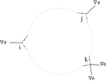
Figure 3: Graphical representation of a general connected diagram coming out from the contraction of the $\psi^{*},\psi$ fields inside the product of vertices $\Gamma_{I,n}$ of Eq. A.

At this point we note that the pairs of fields $\psi^{*},\psi$ in $\Gamma_{I,n}$ may be contracted in a $(n-1)!$ number of ways. Thus, $\Gamma_{I,n}$ consists in a sum of $(n-1)!$ Feynman diagrams. Let $\Gamma_{I,n,\sigma}$ be one of these diagrams. $\sigma$ denotes an arbitrary permutation acting on the set of $(n-1)$ indices $\{2,3,\ldots,n\}$. The expression of $\Gamma_{I,n,\sigma}$ may be obtained by contracting the field $\psi^{*}$ with the field $\psi$ of the $\sigma(2)-$th vertex. Next, the field $\psi^{*}$ of the $\sigma(2)-$th vertex will be contracted with the field $\psi$ of the $\sigma(3)-$th vertex and so on. $\sigma(i)$, $i=1,\ldots,n$ denotes here the result of the permutation of the $i-$th index. Since there are $(n-1)!$ permutations $\sigma$ of this kind, it is easy to check that in this way it is possible to compute all the $(n-1)!$ contributions to $\Gamma_{I,n}$. Let’s check now more in details the structure of each diagram $\Gamma_{I,n,\sigma}$. Due to the particular form of the propagator (58), $\Gamma_{I,n,\sigma}$ will be proportional to the following product of Heaviside $\theta-$functions: $\theta(t_{1}-t_{\sigma(2)})\theta(t_{\sigma(2)}-t_{\sigma(3)})\cdots\theta(t_{\sigma(n)}-t_{1})$. The above product of Heaviside $\theta-$functions enforces the condition:

$$t_{1}>t_{\sigma(2)}>t_{\sigma(3)}>\cdots>t_{\sigma(n)}>t_{1}$$ (61)

Clearly, this sequence of inequalities is impossible. For this reason, the products of Heaviside $\theta-$functions vanishes identically. As a consequence, the determinant of Eq. (54) is trivial, i. e.:

$$\det\left[i\frac{\partial}{\partial t}+(\nabla+ib\nabla\phi)^{2})\right]=1$$ (62)

because all its contributions vanish identically apart from the case $n=0$. This result could be expected from the fact that the field theory given in Eq. (54) is a particular case of a nonrelativistic complex scalar field theory. It is indeed well known that these nonrelativistic field theory give rise to nontrivial determinants gi5 .

References

(1)
R. Brout, Phys. Rep.10C (1974), 1.
(2) F. W. Wiegel, Phys. Rep.16C (1975), 57.
(3) S. Samuel, Phys. Rev.D18 (6) (1978), 1916.
(4) J. Zinn-Justin, Quantum Field Theory and
Critical Phenomena (second edition), Clarendon Press, Oxford 1993.
(5) M. B. Halpern and W. Siegel, Phys. Rev.D 16 (8) (1977), 2486.
(6) F. Ferrari and J. Paturej,
Phys. Lett.B664 (2008), 123.
(7) F. Ferrari and J. Paturej,
Acta
Phys. Pol. B40 (2009), 1383.
(8) F. Ferrari, Jour. Phys. A:
Math. and Gen.36 (2003), 5083, arXiv:hep-th/0302018.
(9) W. Janke and H. Kleinert, Phys. Rev. Lett.75 (1995), 2787.
H. Kleinert, Phys. Rev.D57 (1998),
2264;
H. Kleinert, Phys. Lett.B434 (1998), 74;
H. Kleinert and V. Schulte-Frohlinde, Critical
properties of Theories, World Scientific, Singapore 2001.