Are the input parameters of white-noise-driven integrate & fire neurons uniquely determined by rate and CV?

Abstract

Integrate & fire (IF) neurons have found widespread applications in computational neuroscience. Particularly important are stochastic versions of these models where the driving consists of a synaptic input modeled as white Gaussian noise with mean $\mu$ and noise intensity $D$. Different IF models have been proposed, the firing statistics of which depends nontrivially on the input parameters $\mu$ and $D$. In order to compare these models among each other, one must first specify the correspondence between their parameters. This can be done by determining which set of parameters ($\mu$, $D$) of each model is associated to a given set of basic firing statistics as, for instance, the firing rate and the coefficient of variation (CV) of the interspike interval (ISI). However, it is not clear a priori whether for a given firing rate and CV there is only one unique choice of input parameters for each model. Here we review the dependence of rate and CV on input parameters for the perfect, leaky, and quadratic IF neuron models and show analytically that indeed in these three models the firing rate and the CV uniquely determine the input parameters.

1 Introduction

Stochastic integrate & fire (IF) neurons constitute an important tool in theoretical neuroscience, having been used to address a number of relevant biological problems. For instance, different variants of these models have been employed in the debate on the high variability of the interspike interval (ISI) observed for cortical neurons (Softky and Koch,, 1993; Gutkin and Ermentrout,, 1998). Other problems in which stochastic IF models have been applied include the response to fast signals (Brunel et al.,, 2001; Lindner and Schimansky-Geier,, 2001; Fourcaud-Trocmé et al.,, 2003; Naundorf et al.,, 2005), asynchronous spiking in recurrent networks (Brunel,, 2000), and oscillations of firing activity in systems with spatially correlated noisy driving (Doiron et al.,, 2003, 2004; Lindner et al., 2005b, ).

IF neurons can be classified according to the nonlinearities that govern their subthreshold dynamics. Three simple and important variants are the perfect (PIF), leaky (LIF), and quadratic (QIF) models, in which the subthreshold dynamics is described by a constant, a linear, and a quadratic voltage dependence, respectively. Noisy inputs with different degrees of biological realism have been considered for these models. One simple choice is a white Gaussian input current, corresponding to the so-called diffusion approximation of synaptic spike train input (Holden,, 1976; Ricciardi,, 1977; Tuckwell,, 1989). The PIF with white noise drive (also referred to as the random walk model of neural firing) was first considered by Gerstein and Mandelbrot, (1964). The LIF with a white Gaussian input current has been studied by (Johannesma,, 1968) and afterwards by many other authors (see Holden, (1976); Ricciardi, (1977); Tuckwell, (1989); Burkitt, (2006) and references therein); it is also referred to as Ornstein-Uhlenbeck neuron (Lánský and Rospars,, 1995). White-noise driving in the QIF was studied by Gutkin and Ermentrout, (1998) and Lindner et al., (2003).

The firing statistics of the various IF models may depend sensitively on the specific nonlinearity in the respective model , and so it is not clear at the first glance which model is capable of reproducing which features of the firing statistics of real neurons. For instance, it has been shown that LIF and QIF display rather different phase shifts if driven by a periodic stimulus (Fourcaud-Trocmé et al.,, 2003). Further, the LIF with periodic stimulation can transmit signals of very high frequencies if they are encoded in the noise intensity (Lindner and Schimansky-Geier,, 2001), while the QIF cannot (Naundorf et al.,, 2005). Last but not least, when the strength of the input noise is varied, the LIF can show coherence resonance (CR) (Pakdaman et al.,, 2001; Lindner et al.,, 2002) whereas the PIF and the QIF do not display CR (Lindner et al.,, 2003) (see also below). A thorough comparison of different stochastic IF neurons and the roles of their respective nonlinearities constitutes therefore an interesting and largely open problem.

If one wants to compare two specific IF models one should tune their input parameters (mean and intensity of the input fluctuations) such that the basic firing statistics is the same. A simple choice for the basic firing statistics is the firing rate, quantifying the intensity of the spike train, and the interspike interval’s coefficient of variation (CV), quantifying the irregularity of the spike train. Setting both models in this way in the same firing regime (e.g. low spike rate and high ISI variability), one can then ask for higher statistics (e.g. the power spectrum of the spike train) or for their response characteristics (e.g. to weak periodic stimulation or step currents). The idea for such a tuning tacitly assumes that there is for each of the models at most one input parameter set yielding a desired firing statistics, for instance, rate and CV. At a closer look, however, this is not evident at all: are the input parameters for a white-noise driven IF model indeed uniquely determined if we prescribe certain values of the rate and the CV? This is the question that we address in this paper and we will answer it for the three IF models mentioned above, namely, PIF, LIF, and QIF neurons.

The question discussed here is also related to the problem of parameter estimation for an IF model from experimental data, which has been subject of several studies (see Lánský and Ditlevsen, (2008) and references therein). In one approach, the model parameters are inferred from subthreshold membrane measurements (for a recent reference see Badel et al., (2008)). In another approach, model parameters are estimated using solely the ISI statistics (Tuckwell and Richter,, 1978; Inoue et al.,, 1995; Rauch et al.,, 2003; Camera et al.,, 2004; Shinomoto et al.,, 1999; Ditlevsen and Lansky,, 2005, 2007; Mullowney and Iyengar,, 2008). The latter approach is of importance, since often subthreshold data are not available. Most of these studies consider the leaky IF model. To the best of our knowledge, the problem of the uniqueness of input parameters has been addressed only by Kostal et al., (2007), where it is mentioned without a proof that uniqueness of the input parameters given fixed rate and CV holds for the LIF.

In this paper, we show analytically that rate and CV uniquely determine the input parameters for the three models. We first introduce the models and the statistics studied here (sec. 2). In the main part of the paper (secs. 3-5), we briefly review the rate and CV as functions of the input parameters and then prove the uniqueness of the relation between these parameters and the former statistics. We give an outlook to generalizations of the considered problem in sec. 6.

2 Integrate & fire neuron models

2.1 Definition of the models and relation to the first passage time problem

IF models consist of two ingredients: (i) a one dimensional stochastic ordinary differential equation describing the subthreshold behavior of the membrane potential $V$ as a function of time $t$ and (ii) a fire-and-reset rule. The equation for the membrane potential has the form of a current-balance equation (Burkitt,, 2006):

$$C_{m}\frac{dV}{dt}=I_{\mbox{\tiny{model}}}(V)+I_{\mbox{\tiny{syn}}}(t)+I_{\mbox{\tiny{ext}}}(t),$$ (1)

where $C_{m}$ is the membrane capacitance, $I_{\mbox{\tiny{syn}}}(t)$ and $I_{\mbox{\tiny{ext}}}(t)$ denote the synaptic and injected current, respectively. Here we will consider the case where $I(t)=I_{\mbox{\tiny{syn}}}(t)+I_{\mbox{\tiny{ext}}}(t)$ is a white Gaussian noise current with a constant mean value $\langle I\rangle$ and a correlation function $\langle(I(t)-\langle I\rangle)(I(t^{\prime})-\langle I\rangle)\rangle=2D_{I}\delta(t-t^{\prime})$. The function $I_{model}(V)$ stands for a model-specific current — for instance, a passive leak of the membrane would be described by setting $I_{model}=-[V-V_{0}]/R_{m}$, where $V_{0}$ and $R_{m}$ denote the leak reversal potential and the passive membrane resistance constant, respectively.

The fire-and-reset rule can be expressed as

$$V(t)=V_{th}\Longrightarrow\mbox{ spike at time $t$ and }V\rightarrow V_{r},$$ (2)

i.e., whenever the membrane potential reaches a threshold value $V_{th}$ the neuron fires a spike and there is a reset of its membrane potential to a value $V_{r}$.

It is convenient to make the following changes of variables:

$$v=\frac{V-V_{r}}{V_{th}-V_{r}},\hskip 11.38109ptt\to\frac{t}{\tau_{m}},$$ (3)

where $\tau_{m}=C_{m}R_{m}$ is the membrane time constant and the new variables, $v$ and $t$, are dimensionless. This procedure corresponds to measuring the voltage in units of the difference between threshold and reset (with $V_{r}$ as the reference voltage) and time in units of the membrane time constant.

Defining

$$f_{\mbox{\tiny{model}}}=\frac{R_{m}}{(V_{th}-V_{r})}\left[I_{\mbox{\tiny{model}}}((V_{th}-V_{r})v+V_{r})-I_{\mbox{\tiny{model}}}(V_{r})\right],$$ (4)

$$\mu=\frac{R_{m}}{(V_{th}-V_{r})}\left[\langle I\rangle+I_{\mbox{\tiny{model}}}(V_{r})\right],$$ (5)

and

$$D=\frac{D_{I}R_{m}^{2}}{\tau_{m}(V_{th}-V_{r})^{2}},$$ (6)

we can recast Eq. (1) into the form:

$$\dot{v}=f_{\mbox{\tiny{model}}}(v)+\mu+\sqrt{2D}\xi(t),$$ (7)

which is the equation that we will work with in the remainder of this work. The parameters $\mu$ and $D$ are called input parameters, i.e. they represent the mean and the intensity of the fluctuating input in our nondimensional model. Note that they are linearly related to the physiological input parameters $\langle I\rangle$ and $D_{I}$ via Eq. (5) and Eq. (6). The function $\xi(t)$ is a zero-mean white Gaussian noise with $\langle\xi(t)\xi(t^{\prime})\rangle=\delta(t-t^{\prime})$. In the nondimensional formulation Eq. (7), the reset and threshold values, $v_{r}$ and $v_{th}$, are given by zero and one, respectively. For better applicability of our results, we will keep $v_{r}$ and $v_{th}$ in all resulting formulas and equations.

If one neglects any voltage dependence of the right-hand side in Eq. (7), one deals with a perfect integrator and the respective IF model is called a perfect integrate & fire (PIF) neuron:

$$f_{\mbox{\tiny{PIF}}}=0,\hskip 22.76219pt\mu>0,\hskip 22.76219ptv_{th}=1,\hskip 22.76219ptv_{r}=0.$$ (8)

If a leak current is taken into account, $f(v)$ becomes a linear function (by construction, any additive constant is lumped into the mean input $\mu$). In this case, we deal with a leaky integrate & fire (LIF) neuron which is the most often studied and used IF model to date:

$$f_{\mbox{\tiny{LIF}}}=-v,\hskip 22.76219pt\mu\in(-\infty,\infty),\hskip 22.76219ptv_{th}=1,\hskip 22.76219ptv_{r}=0.$$ (9)

Another IF model, the quadratic integrate & fire (QIF) model also fits into the framework of Eq. (7) although in its derivation $v$ is not a voltage but a more abstract variable. Higher nonlinearities in the current-balance Eq. (1) come along by voltage-dependent conductances and additional variables like gating variables (e.g. in the classical Hodgkin-Huxley model) or effective recovery variables (e.g. in the Morris-Lecar model). A wide class of neurons (type I neurons) described by such multidimensional dynamical systems shows a behavior associated with a saddle-node bifurcation (Rinzel and Ermentrout,, 1989) in these multidimensional models. For these neurons, the dynamics close to the bifurcation is governed by one slow variable only which is the variable $v$ in our general IF model Eq. (7). The nonlinearity corresponding to the normal form of a saddle-node bifurcation is a quadratic function. Furthermore, for this specific dynamics the behavior is governed by the slow motion close to $v=0$ and threshold as well as reset values do not matter if taken far away from the origin. For simplicity, they are commonly taken at infinity. Thus the dynamics of a QIF model is described by the following setup:

$$f_{\mbox{\tiny{QIF}}}=v^{2},\hskip 22.76219pt\mu\in(-\infty,\infty).\hskip 22.76219ptv_{th}=\infty,\hskip 22.76219ptv_{r}=-\infty.$$ (10)

It is useful to interpret Eq. (7) as describing a Brownian particle of position $v$ undergoing overdamped motion in a potential $U{\mbox{\tiny{model}}}$ such that

$$-\frac{dU{\mbox{\tiny{model}}}}{dv}=f_{\mbox{\tiny{model}}}+\mu.$$ (11)

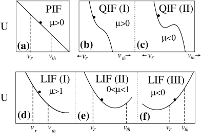
Figure 1: Potentials for the different models (cf. Eq. (11)). The PIF (a) is only defined in the tonic firing regime ($\mu>0$) while the QIF ((b) and (c)) can be in the tonic (QIF I in (b)) or in the noise-induced (QIF II in (c)) firing regimes. The LIF displays tonic firing (LIF I in (d)) for $\mu>1$ and two different noise-induced firing regimes ((e) and (f)) for which we distinguish the cases where the potential minimum lays between $v_{r}$ and $v_{th}$ (e) and where the minimum is to the left of the reset point (f). In the latter case, the potential picture allows for a simple interpretation of the high variability ($CV>1$) under moderate noise intensity: short ISIs occur when the particle moves directly from $v_{r}$ to $v_{th}$, while long ISIs correspond to realizations in which the particle first performs an excursion to the potential minimum and then hits threshold.

In this analogy, the ISI of the respective neuron model turns into the first-passage time of the Brownian particle starting at the reset point towards the threshold point. Depending on the model and, in particular, on the value of $\mu$, the passage can occur already without noise (tonic firing regime) or must be assisted by fluctuations (noise-induced firing regime). The tonic regime can be most easily illustrated in case of the PIF where the particle just slides down an inclined plane from reset to threshold (see Fig. 1a) , whereas noise is needed to reach the threshold whenever there is a barrier present between reset and threshold (QIF for $\mu<0$, see Fig. 1c) or right at the threshold (LIF, $\mu<1$, see Figs. 1(e) and (f)). Note that the parameter $\mu$ has different meaning in the three models. In the PIF it attains only positive values and sets merely the time scale of the system. In the QIF it is a bifurcation parameter: at negative $\mu$ the potential attains one minimum whereas for positive $\mu$ the potential is a nonlinear but monotonic function. In the LIF, the bifurcation from tonic to noise-induced firing takes place at $\mu=1$. As we will see, for the firing statistics of the LIF it is furthermore useful to distinguish the case where $\mu<0$: here large values of the CV can be easily interpreted in light of the specific properties of the potential (see below).

2.2 Measures

The spike train is defined as a sum of delta functions at the spiking times (Gerstner and Kistler,, 2002), i.e., the time instants when the voltage reaches the threshold and the fire-and-reset rule is applied (cf. Fig. 2):

$$y(t)=\displaystyle\sum_{j}\delta(t-t_{j}).$$ (12)

In Eq. (12), $t_{j}$ stands for the instant when the $j$-th spike is triggered. Fig. 2 depicts the time evolution of the subthreshold voltage as described by one of the models we address and the corresponding spike train. The time intervals $T_{j}=t_{j}-t_{j-1}$ between two immediately subsequent spikes are the ISIs.

Figure 2: Subthreshold voltage dynamics and corresponding spike train as from a simulation of Eq. (7) and Eq. (8) (PIF) with parameters $\mu=0.9$ and $D=0.006$. Note the high degree of regularity of the spike train, characteristic of the PIF model under strong mean input with low noise intensity.

The spike trains considered here are stationary stochastic point processes. The firing rate $r$ of such a process can be defined as the inverse mean ISI:

$$r=\frac{1}{\langle T\rangle}.$$ (13)

The coefficient of variation ($CV$) of the ISI is defined as:

$$CV=\frac{\sqrt{\langle\Delta T^{2}\rangle}}{\langle T\rangle},$$ (14)

where $\langle\Delta T^{2}\rangle=\langle T^{2}\rangle-\langle T\rangle^{2}$ is the variance of the ISI distribution. The CV can be regarded as the relative standard deviation of the ISI. For comparison, a perfectly periodic spike train would have zero CV while a Poissonian spike train possesses a CV of one.

As regards experimentally measured values of the rate and the CV, we note that all nondimensional values of rates discussed in the following translate into the former by $r_{real}=r/\tau$. For example, for a membrane time constant $\tau=R_{m}C_{m}=10$ms nondimensional IF rates of $r=0.01,0.1,$ and $1$ correspond to firing rates of $r_{real}=1,10,$ and $100$ Hz. Note that the CV (being a relative standard deviation) does not change upon a time transformation, i.e. $CV_{real}=CV$.

2.3 General form of the differential equations governing the contour lines

Analytical formulas for the moments $\langle T^{n}\rangle$ of the first passage time from $x_{-}$ to $x_{+}$ in an arbitrary potential $U(x)$ were derived by Pontryagin et al., (1933). Simplifications of these quadrature formulas as well as sum formulas for specific cases have been put forward by many authors (for a selection, see, for instance, (Holden,, 1976; Ricciardi,, 1977; Ricciardi and Sacerdote,, 1979; Tuckwell,, 1988; Colet et al.,, 1989; Bulsara et al.,, 1994, 1996; Lindner et al.,, 2002, 2003)). The first two moments determine the rate and CV, according to Eqs. (13) and (14). For completeness, we write the expressions for these moments here:

$$\langle T\rangle=\frac{1}{D}\int_{x_{-}}^{x_{+}}dxe^{U(x)/D}\int_{-\infty}^{x}dye^{-U(y)/D}$$ (15)

and

$$\langle T^{2}\rangle=\frac{2}{D^{2}}\int_{x_{-}}^{x_{+}}dxe^{U(x)/D}\int_{-\infty}^{x}dye^{-U(y)/D}\times\int_{y}^{x^{+}}dze^{U(z)/D}\int_{-\infty}^{z}dve^{-U(v)/D}.$$ (16)

In this paper we will study the rate and CV of the three models as functions of the input parameters, $\mu$ and $D$. In particular, we are interested in the curves for which $F(D,\mu)=\mbox{const}$ ($F$ denotes either $r$ or CV), i.e., the contour lines of the surfaces $F(D,\mu)$ over the $(D,\mu)$ parameter plane. The contour lines can be obtained if one observes that $dF=0$ along them. Since $dF=(\partial F/\partial D)dD+(\partial F/\partial\mu)d\mu$, one concludes that the following differential equations for functions $\mu_{F}(D)$ or $D_{F}(\mu)$ parametrize the contour lines:

$$\frac{d\mu_{F}}{dD}=-\frac{\partial F/\partial D}{\partial F/\partial\mu},$$ (17)

$$\frac{dD_{F}}{d\mu}=-\frac{\partial F/\partial\mu}{\partial F/\partial D},$$ (18)

where $F\in\{r,CV\}$, provided that $\partial{F}/\partial{\mu}\neq 0$ and $\partial{F}/\partial{D}\neq 0$, respectively. We note that these conditions are not necessarily satisfied in the whole $(D,\mu)$ parameter space of the models we address. For instance, for the PIF we have in fact $\partial{r}/\partial{D}=0$ for all valid pair $(D,\mu)$. However, for the three models studied here, at any point $(D,\mu)$ of parameter space at least one of these conditions is satisfied.

If for any pair $(r,CV)$ the respective contour lines $\mu_{r}(D)$ and $\mu_{CV}(D)$ intersect at most once, then rate and CV determine uniquely the parameters of the respective IF model. In the following sections we will show that this is indeed the case for the PIF, LIF, and QIF.

3 Perfect integrate & fire neuron

The mean and variance of the ISI are given by (Holden,, 1976; Tuckwell,, 1988; Bulsara et al.,, 1994; Burkitt,, 2006):

$$\langle T\rangle=\frac{v_{th}-v_{r}}{\mu},\hskip 14.22636pt\langle\Delta T^{2}\rangle=\frac{2D(v_{th}-v_{r})}{\mu^{3}}.$$ (19)

We stress that $\mu>0$ for the PIF; otherwise all moments of the ISI diverge. For this model the expressions for rate and CV are quite simple:

$$r=\frac{\mu}{v_{th}-v_{r}},\hskip 14.22636ptCV^{2}=\frac{2D}{\mu(v_{th}-v_{r})}.$$ (20)

Moreover, the contour lines for the rate and the CV can be explicitely calculated (without resorting to the differential equations Eq. (17) and Eq. (18)):

$$\mu_{r_{0}}(D)=r_{0}(v_{th}-v_{r}),\;\;\;\;\mu_{CV_{0}}(D)=\frac{2D}{(v_{th}-v_{r})CV_{0}^{2}}.$$ (21)

We briefly review the behavior of rate and CV as functions of $\mu$ and $D$ and then show that rate and CV uniquely fix the system’s parameters.

3.1 Rate and CV and their contour lines in the ($D,\mu$) plane for the PIF

The rate and CV are shown in Figs. 3(a) and 3(b) as functions of the parameters $\mu$ and $D$. The rate is a linear function of $\mu$ and, remarkably, does not display any dependence on $D$. This is a unique property of the PIF model. The $CV$ depends linearly on $\sqrt{D/\mu}$, and can therefore attain values in the whole range $0<CV<\infty$.

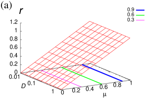
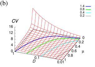
Figure 3: Rate (a) and CV (b) as a function of the parameters $\mu$ and $D$ for the PIF model. The rate is a simple increasing function of the mean input and does not depend on the noise intensity. The CV is proportional to $\sqrt{D/\mu}$ (cf. Eq. (20)). In (c) we show contour lines corresponding to three different values of the rate (dashed lines) and to four different values of the CV (solid lines with symbols). If for a given pair of rate and CV there is only one pair of input parameters $(\mu,D)$, there should be only one intersection point for two specific (dashed and solid) contour lines. The uniqueness of this correspondence can be explicitely shown for the PIF (see Eq. (22) and Eq. (23)).

Fig. 3(c) shows contour lines for different rates and CVs, which are for both measures just straight lines. Generally, the variability of the PIF’s spike train increases by decreasing the mean input and increasing the noise intensity, which is quite intuitive.

3.2 Uniqueness of the model parameters for a given rate and CV for the PIF

In the fairly simple case of the PIF, Eq. (20) can be readily inverted to yield $\mu$ and $D$ as a function of rate and CV:

$$\mu=r(v_{th}-v_{r}),$$ (22)

$$D=\frac{r(v_{th}-v_{r})^{2}CV^{2}}{2}.$$ (23)

Eqs. (22) and (23) define a mapping $(r,CV)\mapsto(D,\mu)$, implying that for any pair $(r,CV)$ there exists one and only one pair $(D,\mu)$.

4 Leaky integrate & fire neuron

For the LIF, the mean and variance of the ISIs are (Ricciardi,, 1977; Tuckwell,, 1988; Lindner et al.,, 2002):

$$\langle T\rangle=\sqrt{\pi}\int_{a}^{b}dye^{y^{2}}\mbox{ erfc}(y),$$ (24)

$$\langle\Delta T^{2}\rangle=2\pi\int_{a}^{b}dze^{z^{2}}\int_{z}^{\infty}dye^{y^{2}}\mbox{erfc}^{2}(y),$$ (25)

where

$$a=(\mu-v_{th})/\sqrt{2D}\mbox{ and }b=(\mu-v_{r})/\sqrt{2D}.$$ (26)

From these expressions and the general relations Eqs. (17) and Eq. (18), one can derive the differential equations that govern the contour lines as follows:

$$\frac{d\mu_{r}}{dD} = \frac{b-a}{v_{th}-v_{r}}\left(\frac{be^{b^{2}}\mbox{ erfc}(b)-ae^{a^{2}}\mbox{ erfc}(a)}{e^{b^{2}}\mbox{ erfc}(b)-e^{a^{2}}\mbox{ erfc}(a)}\right),$$ (27)

$$\frac{d\mu_{CV}}{dD} = \left(\frac{b-a}{v_{th}-v_{r}}\right)\left[a\left(1-\mathbb{F}(a,b)\right)^{-1}+b\left(1-\frac{1}{\mathbb{F}(a,b)}\right)^{-1}\right],$$ (28)

$$\mathbb{F}(a,b) = \frac{\int_{a}^{b}dxe^{x^{2}}\mbox{erfc}(x)e^{b^{2}}\int_{b}^{\infty}dye^{y^{2}}\mbox{erfc}^{2}(y)-2\int_{a}^{b}dze^{z^{2}}\int_{z}^{\infty}dye^{y^{2}}\mbox{erfc}^{2}(y)e^{b^{2}}\mbox{erfc}(b)}{\int_{a}^{b}dxe^{x^{2}}\mbox{erfc}(x)e^{a^{2}}\int_{a}^{\infty}dye^{y^{2}}\mbox{erfc}^{2}(y)-2\int_{a}^{b}dze^{z^{2}}\int_{z}^{\infty}dye^{y^{2}}\mbox{erfc}^{2}(y)e^{a^{2}}\mbox{erfc}(a)},$$ (29)

$$\frac{dD_{CV}}{d\mu} = \left[\frac{d\mu_{CV}}{dD}\right]^{-1}.$$ (30)

We will first recall some properties of rate and CV, most but not all of which have been already discussed elsewhere (Pakdaman et al.,, 2001; Lindner et al.,, 2002).

4.1 Rate and CV and their contour lines in the ($D,\mu$) plane for the LIF

Rate and CV as functions of $\mu$ and $D$ are shown in Fig. 4. As seen in Fig. 4(a), the rate is an increasing function of $\mu$ for fixed $D$ and an increasing function of $D$ for fixed $\mu$. In the zero-noise limit, the rate is zero for $\mu<v_{th}$ and increases monotonically for $\mu>v_{th}$ according to the well-known rate of a deterministic LIF model $r^{-1}=\ln[(\mu-v_{r})/(\mu-v_{th})]$ Gerstner and Kistler, (2002).

The behavior of the CV is much richer (see Fig. 4(b)). In particular, the LIF model displays coherence resonance (CR) (Pakdaman et al.,, 2001; Lindner et al.,, 2002): for fixed $\mu<v_{th}$, the CV exhibits a minimum at a finite value of $D$. Coherence resonance thus corresponds to the phenomenon by which noise has the counter-intuitive effect of increasing the regularity of the spike train. For the LIF, a pronounced CR is observed for a mean input $\mu$ close to but smaller than the threshold ($\mu\lesssim v_{th}$).

The CV for the LIF can exceed unity (this feature is also displayed by the PIF but not by the QIF). Loosely speaking, such a regime corresponds to a firing activity more irregular than in the Poissonian regime ($CV=1$). This high variability is associated to short ISIs occurring relatively frequently, but long ISIs being also likely. When $\mu<0$, a simple interpretation can be made in terms of the Brownian particle in a parabolic potential. As shown in Fig. 1(f), in this case, both $v_{r}$ and $v_{th}$ are larger than the value of $v$ at which the potential attains its minimum. The short ISIs then correspond to the cases when the particle heads directly from $v_{r}$ to $v_{th}$, while the long ones correspond to the particle first going to the minimum of the potential and then performing its excursion to $v_{th}$.

Independently of $D$, if $\mu\rightarrow-\infty$ the firing becomes Poissonian ($CV=1$). In the opposite limit of $\mu\to\infty$, the firing is perfectly regular ($CV=0$). At least for large noise intensity, the CV exceeds unity, as discussed above. Therefore, for fixed and sufficiently large value of the noise intensity we observe a maximum of the CV with respect to $\mu$. This is an interesting feature of the LIF model - not shared by PIF or QIF - which to our knowledge has not been described so far. It implies that, given a fixed level of the input fluctuations, the degree of irregularity of the spike train is maximal (maximized incoherence) for a finite value of the mean input. We note that another type of maximized incoherence has been described for the LIF with an additional absolute refractory period by Lindner et al., (2002). In that case, the CV achieves a maximal value for a finite noise intensity when the mean input is fixed.

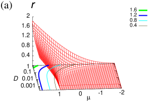
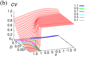
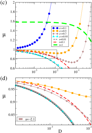
Figure 4: Rate (a) and CV (b) as a function of the parameters $\mu$ and $D$ for the LIF model. In (c) we show contour lines for three values of the rate (dashed lines) and four values of the CV (solid lines with symbols). Note the nonmonotonic character of the CV’s contour lines $\mu_{CV_{0}}(D)$. The rectangular region marked in (c) is magnified in (d). Also plotted in (d) is one curve (brown thick line) of the type $a=\mbox{const}$ [cf. Eq. (26)], corresponding to a contour line for the ISI statistics in the Poissonian firing limit. Contour lines in this limit for the rate ($r=0.01$, black dashed line) and CV ($CV=0.95$, magenta triangles) are very close to this line and, consequently, to each other.

As also shown in Fig. 4(b), the contour lines for the CV display nonmonotonicities with respect to both parameters. The contour lines at which the CV is smaller than 1 display nonmonotonic behavior with respect to $D$, whereas the ones corresponding to CV larger than 1 are nonmonotonic functions of $\mu$ (see, for instance, the contour line $CV=1.1$). Fig. 4(c) shows contour lines for rate and CV in a range of physiological interest.

We also observe in Fig. 4(d) that the contour lines of rate and CV are very close to each other in the region of small $D$ and $\mu<v_{th}$ (see especially contour lines $r=0.01$ and $CV=0.95$). The reason is that in this region we approach the Poissonian firing limit, in which case the dynamics of the model depends on the threshold value — hence on $a$ — but not on the reset value — hence not on $b$ (see e.g. Ditlevsen and Lansky, (2005) and references therein). For a small but finite value of $D$ and $\mu<v_{th}$, the dependence on the parameter $b$ that distinguishes the contour lines of rate and CV is very weak which is the reason why these contour lines will be very close to each other. Assuming an exclusive dependence on $a$, we obtain a universal contour line for all ISI statistics (this holds strictly true only in the Poissonian limit) by setting $a=$const . One such line (with $a=-2.1$ extracted from the rate curve for $r=0.01$ at $D=0.001$) is shown in Fig. 4(d): indeed, the corresponding contour lines of rate and CV are very close to this line.

Thus, as the firing regime approaches the Poissonian limit, the actual determination of the intersections of the contour lines becomes a practically more difficult task. Also it becomes less clear whether there is only intersection point or not. In view of this particular (numerical) uncertainty, but also in view of the nonmonotonic behavior of the contour lines $\mu_{CV}$ as functions of $D$ (for $\mu<v_{th}$) and $\mu$ (for strong noise), it is desirable to gain certainty about whether rate and CV uniquely determine $D$ and $\mu$ in the LIF model.

4.2 Uniqueness of the model parameters for a given rate and CV for the LIF

Our strategy to show that the model parameters are uniquely determined for a given rate and CV comprises two steps. First, we demonstrate that each contour line for the rate is unique. Second, we prove that the CV is a monotonic function along any rate contour line. The second step can be simplified by noting that the CV is the ratio between the square root of the variance $\sigma^{2}=\langle\Delta T^{2}\rangle$ and the mean $\langle T\rangle$. Since the mean is invariant in any contour line for the rate, it suffices to show that the $\sigma^{2}$ is a monotonic function along any such contour line. In other words, it suffices to show that the directional derivative of $\sigma^{2}$ along the tangent of the contour line for the rate is strictly positive .

4.2.1 Uniqueness of contour lines for the rate

Let us prove that the contour line for a specific value of the rate $r(D,\mu)=r_{0}$ is one single connected curve. The proof comprises three steps: First, for any point $(D,\mu)\in\mathbb{R}^{+}\times\mathbb{R}$ we can locally construct a contour line $\mu_{r_{0}}(D)$ parametrized by $D$ such that $r(D,\mu_{r_{0}}(D))=r_{0}$. This is possible locally by virtue of the implicit function theorem since, as shown in Appendix B, $\partial{r}/\partial{\mu}>0$ for all $(D,\mu)\in\mathbb{R}^{+}\times\mathbb{R}$. Of course, the specific value of the rate, $r_{0}$, will depend on the point $(D,\mu)$. Second, we can extend $\mu_{r_{0}}(D)$ to the whole domain $D\in\mathbb{R}^{+}$ by connecting neighborhoods of this domain. This could be made impossible if $\mu_{r_{0}}(D)$ diverges at finite D. We rule out this possibility by noting that it is not consistent with the limit values of the rate at $\mu=\pm\infty$. Indeed, as we show in Appendix B, the limit of the rate is zero (for $\mu\to-\infty$) or $\infty$ (for $\mu\to\infty$), values which are not attained by the rate for any positive $D$ and finite $\mu$. Hence no contour line starting within the domain can approach the boundary $\pm\infty$ at finite $D$ and thus there cannot be a divergence of the contour line at finite $D$. Hence $\mu_{r_{0}}(D)$ will describe a single connected line for the whole domain $D\in\mathbb{R}^{+}$. Third, we show that the graph of $\mu_{r_{0}}(D)$ contains all points $(D,\mu)$ with $r(D,\mu)=r_{0}$. In fact, if a point $(D^{*},\mu^{*})$ not belonging to the graph of $\mu_{r_{0}}(D)$ exists such that $r(D^{*},\mu^{*})=r_{0}$, then the condition $\partial{r}/\partial{\mu}>0$ must necessarily be violated along the vertical line $D=D^{*}$. This completes the proof that the contour lines for rate are single (connected) curves.

4.2.2 Proof that $\sigma^{2}$ is a monotonic function along the rate contour lines

Along a contour line of the rate, the mean ISI is fixed by definition and thus the CV can only vary due to changes in the variance $\sigma^{2}$. Thus if we show that the variance increases monotonically as we move along the contour line in the direction of increasing $D$, we will have also shown that the CV increases monotonically if we move along the contour line in this direction.

The monotonicity of $\sigma^{2}$along the rate contour lines is expressed by

$$\nabla\sigma^{2}\cdot{\bf v_{t}}>0,$$ (31)

where ${\bf v_{t}}$ is a vector which is tangent to these contour lines and $\nabla$ denotes the gradient in $(D,\mu)$ space. In order to show that Eq. (31) holds, let us first determine ${\bf v_{t}}$. Along the rate contour lines, the differential equation Eq. (17) with $F=r$ holds true; its right-hand side is needed for an expression of the tangent vector of the rate contour lines appearing in Eq. (31):

$${\bf v_{t}}={\bf e}_{D}+\frac{d\mu_{r}}{dD}{\bf e}_{\mu}$$ (32)

where ${\bf e}_{D}$ and ${\bf e}_{\mu}$ are the respective unit vectors. The relation to be shown, Eq. (31), thus corresponds to

$$\frac{\partial\sigma^{2}}{\partial D}+\frac{\partial\sigma^{2}}{\partial\mu}\frac{d\mu_{r}}{dD}>0.$$ (33)

It is much simpler to express the derivatives on the left hand side of Eq.(33) in terms of coordinates $a$ and $b$ rather than $D$ and $\mu$. Using Eqs. (25) and (26), we obtain

$$\frac{\partial\sigma^{2}}{\partial D}=\frac{2\pi(b-a)^{2}}{(v_{th}-v_{r})^{2}}\left(-be^{b^{2}}\int_{b}^{\infty}dye^{y^{2}}\mbox{erfc}^{2}(y)+ae^{a^{2}}\int_{a}^{\infty}dye^{y^{2}}\mbox{erfc}^{2}(y)\right)$$ (34)

and

$$\frac{\partial\sigma^{2}}{\partial\mu}=\frac{2\pi(b-a)}{v_{th}-v_{r}}\left(e^{b^{2}}\int_{b}^{\infty}dye^{y^{2}}\mbox{erfc}^{2}(y)-e^{a^{2}}\int_{a}^{\infty}dye^{y^{2}}\mbox{erfc}^{2}(y)\right).$$ (35)

Inserting Eqs. (27, 34-35) into Eq.(33), and performing straightforward algebra, we write the latter as:

$$\frac{2\pi(b-a)^{3}e^{a^{2}+b^{2}}\mbox{erfc}(a)\mbox{erfc}(b)}{(v_{th}-v_{r})^{2}(e^{a^{2}}\mbox{erfc}(a)-e^{b^{2}}\mbox{erfc}(b))}\left(\int_{a}^{\infty}dye^{y^{2}}\frac{\mbox{erfc}^{2}(y)}{\mbox{erfc}(a)}-\int_{b}^{\infty}dye^{y^{2}}\frac{\mbox{erfc}^{2}(y)}{\mbox{erfc}(b)}\right)>0.$$ (36)

This inequality holds true for all $a<b$ since the two functions $e^{a^{2}}\mbox{erfc}(a)$ and $\int_{a}^{\infty}dx\;\mbox{erfc}^{2}(x)/\mbox{erfc}(a)$ (differences of which appear in Eq. (36)) are monotonically decreasing functions of $a$ as we prove in the Appendix A. We have thus proven Eq. (33) and hence we have shown that the variance of the ISI always increases as we go along the constant rate contour line in the direction of increasing noise intensity. This completes our proof of the uniqueness of parameters determined by prescribed values of the rate and the CV.

5 Quadratic integrate & fire neuron

For the QIF, one has (Lindner et al.,, 2003):

$$\langle T\rangle=\left(\frac{9}{D}\right)^{1/3}I(\alpha)\mbox{, }\hskip 11.38109ptI(\alpha)=\int\limits_{-\infty}^{\infty}dx\;e^{-\alpha x-x^{3}}\int\limits_{-\infty}^{x}dy\;e^{\alpha y+y^{3}},$$ (37)

$$\langle\Delta T^{2}\rangle=\left(\frac{9}{D}\right)^{2/3}\int_{-\infty}^{\infty}dxe^{-\alpha x-x^{3}}\int_{x}^{\infty}dye^{-\alpha y-y^{3}}\left[\int_{-\infty}^{x}dze^{\alpha z+z^{3}}\right]^{2},$$ (38)

$$\alpha=\left(\frac{3}{D^{2}}\right)^{1/3}\mu.$$ (39)

For this model, the following scaling relations (Lindner et al.,, 2003) facilitate the determination of the contour lines in parameter space for rate and CV:

$$r(\mu,D)=\sqrt{|\mu|}r(\frac{\mu}{|\mu|},|\mu|^{-3/2}D),$$ (40)

$$CV(\mu,D)=CV(\frac{\mu}{|\mu|},|\mu|^{-3/2}D).$$ (41)

The scaling relation Eq. (41), together with the monotonicity of the CV for $\mu=\pm 1$ (see Lindner et al., (2003)), implies that (for $\mu=\pm 1$) a certain value of the CV (say, $CV_{0}$) determines uniquely the noise intensity D which we call $\bar{D}$. With this observation, the contour lines for the CV for arbitrary $\mu$ can be explicitely written:

$$\mu_{cv}(D)=\frac{\mu}{|\mu|}\left(\frac{D}{\bar{D}}\right)^{2/3}.$$ (42)

For the rate, $\bar{D}$ can be regarded as a parameter of the curve $\mu_{r}(D)$: from the above definition of $\bar{D}$ and from the scaling relation for the rate Eq. (40) we can infer that

$$\mu(\bar{D})=\frac{\mu}{|\mu|}\left(\frac{r_{0}}{r(\frac{\mu}{|\mu|},\bar{D})}\right)^{2},\;\;\;D(\bar{D})=\bar{D}\left(\frac{r_{0}}{r(\frac{\mu}{|\mu|},\bar{D})}\right)^{3}$$ (43)

describe all the points on the curve $\mu_{r}(D)$ which we get by varying $\bar{D}$.

We will now recall some properties of rate and CV which have been already discussed by Lindner et al., (2003).

5.1 Rate and CV and their contour lines in the ($D,\mu$) plane for the QIF

Rate and CV as a function of $\mu$ and $D$ are shown in Fig. 5. The behavior of the rate is similar to the case of the LIF. Here again it is a monotonically increasing function of $\mu$ for fixed $D$ and monotonically increasing function of $D$ for fixed $\mu$. A noticeable difference arises in the zero-noise limit and close to the bifurcation at $\mu=0$: the rate for the QIF is also strictly zero if $\mu\leq 0$ but, differently from what is observed for the LIF, it increases proportionally to the square root of $\mu$ for small positive $\mu$.

In clear contrast to the LIF and PIF, the CV for the QIF is bounded in the interval $0<CV<1$. Moreover, here the CV is a strictly monotonic function of both $D$ and $\mu$. For fixed $D$, it decreases with increasing $\mu$ and, for fixed positive (negative) $\mu$, it increases (decreases) with increasing $D$. Therefore, coherence resonance does not occur for this model.

Fig. 5c shows some contour lines for rate and CV in the physiologically relevant region of the parameter space. We emphasize that for the QIF the contour lines of the CV are monotonic functions of both $D$ and $\mu$.

As shown in Fig. 5d, the contour lines of rate and CV are in close vicinity in the region of small $D$ and $\mu<0$, analogously to what is observed for the LIF. In this Poissonian firing limit, the dynamics of the QIF depends most strongly on the ratio of potential barrier and noise intensity (Lindner et al.,, 2003) which can be interpreted as a rescaled barrier

$$\Delta u=\frac{4|\mu|^{3/2}}{3D}.$$ (44)

For instance, the firing rate in the Poissonian limit (corresponding to the Kramers rate out of the cubic potential well) depends on this barrier exponentially and has only a mild additional dependence on $\mu$ via a prefactor (Lindner et al.,, 2003)

$$r=\sqrt{|\mu|}/\pi e^{-\Delta u},\;\;\;\Delta u\gg 1.$$ (45)

The line $\Delta u=$const is indeed close to both the contour lines of rate and of CV in the Poissonian limit (cf. brown line in Fig. 5d). Note that Eq. (45) offers another, more accurate approximation, to the contour line of the rate in the Poissonian firing regime. This line is, however, very close to the line obtained from a constant barrier $\Delta u=$const.

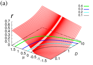
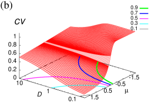
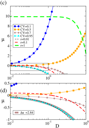
Figure 5: Rate (a) and CV (b) as a function of the parameters $\mu$ and $D$ for the QIF model. In (c) we show contour lines for three values of the rate (dashed lines) and four values of the CV (solid lines with symbols) as indicated. The rectangular region in (c) is magnified in (d). In (d) we also plot the one curve (brown thick line) governing all ISI statistics in the Poissonian regime with $\Delta u(\mu,D)=2.84$ (corresponding to the value at $D=0.1,\mu=-0.36$) resulting in $\mu=-(0.75D\Delta u)^{2/3}$ (cf. the discussion around Eq. (44)). The more sparse grid in the region close to $\mu=0$ in (a, b) is due to the way we generated the points and does not reflect any property of the surfaces $r(D,\mu)$ and $CV(D,\mu)$.

5.2 Uniqueness of the model parameters for a given rate and CV for the QIF

We will consider as given that the $CV(1,\bar{D})$ ($CV(-1,\bar{D})$) is a monotonically increasing (decreasing) function of $\bar{D}$; this was previously demonstrated by limit cases and by numerical evaluation of the integrals (Lindner et al.,, 2003). From these properties we can conclude: for negative (positive) $\mu$, decreasing (increasing) the CV from 1 (0) to $3^{-1/2}$, the parameter $\bar{D}$ changes monotonically from 0 to infinity implying that each CV between 0 and 1 has one unique contour line parametrized by the sign of $\mu$ and the value of $\bar{D}$ (see Eq.(42)). The value $\mu=0$ is a special case where the CV attains exactly the value at the boundary between the regimes $\mu<0$ and $\mu>0$, namely, CV=$3^{-1/2}$ (Sigeti and Horsthemke,, 1989).

If we can show that the rate or equivalently the mean ISI changes monotonically along the contour lines of the CV, then there is at most one intersection for a given pair of CV and rate and thus the mapping of rate and CV to $\mu$ and $D$ is unique. Note that although our argument is similar to the one used for the LIF, we will consider the change in the mean ISI along the curve of constant CV and not the change in CV (or variance) along a curve of constant rate as we did for the LIF.

The directional derivative of the mean ISI along the CV contour line reads

$$\nabla\langle T\rangle\cdot{\bf v_{t}}=\frac{\partial\langle T\rangle}{\partial D}+\frac{\partial\langle T\rangle}{\partial\mu}\frac{d\mu_{CV}}{dD}.$$ (46)

From Eq. (42), we obtain:

$$\frac{d\mu_{cv}}{dD}=\frac{\mu}{|\mu|}\frac{2}{3}D^{-1/3}\bar{D}^{-2/3}.$$ (47)

Using this expression and Eqs. (37) and (39), one can rewrite the directional derivative as follows:

$$\nabla\langle T\rangle\cdot{\bf v_{t}} = -\frac{1}{3D}\langle T\rangle-\frac{2}{D^{2}}\frac{\partial I(\alpha)}{\partial\alpha}\left[\mu-\frac{\mu}{|\mu|}\left(\frac{D}{\bar{D}}\right)^{2/3}\right]$$ (48)

where we have used the auxiliary function $I(\alpha)$ from Eq. (37). The expression in the brackets vanishes by definition since it equals $\mu-\mu_{CV}$ according to Eq. (42). Hence we find that the last term is truly zero and thus the directional derivative of the mean ISI along the contour lines of the CV is negative throughout the $(\mu,D)$ plane

$$\nabla\langle T\rangle\cdot{\bf v_{t}} = -\frac{1}{3D}\langle T\rangle<0.$$ (49)

We have thus shown that (i) for each CV between 0 and 1 there exists exactly one contour line and (ii) the mean ISI decreases always as we go along these contour lines in direction of increasing noise intensity. Hence, each mean ISI is at most represented once on a contour line of the CV and thus for each pair of rate and CV values there is at most one pair $(\mu,D)$.

6 Conclusions

To summarize, we have reviewed the behavior of rate and CV as functions of the input parameters for three different IF models. As the central result of our paper, we have shown that these statistics uniquely determine the input parameters for the models studied. This sets a framework for systematic comparison of these models: they can be compared on an equal footing when their parameters are tuned so as to yield the same rate and CV. Reports on these comparisons will be published elsewhere.

It is tempting to consider the general IF model with white noise input: do rate and CV determine the input parameters for an arbitrary nonlinear function $f_{\mbox{\tiny{model}}}(v)$ or equivalently for an arbitrary nonlinear potential $U(v)$? Unfortunately, so far no general procedure to show the uniqueness of input parameters is known. What we showed in this paper relied on model-specific properties of the ISI moments for the PIF, LIF, and QIF. Approaches to the uniqueness problem based on the general formulas for the moments of the first-passage time Eq. (15) and Eq. (16) could lead to conditions on the potential $U(v)$ and the reset and threshold values of the IF model; however, we have not made any progress in this direction yet. We note that it may still be worth the effort to prove the uniqueness of parameter values for a given rate and CV for other specific neuron models of the IF type. One such a case is the exponential IF model (Fourcaud-Trocmé et al.,, 2003), which has been successfully used to describe pyramidal neurons activity (Badel et al.,, 2008).

Another and more complicated open problem is to check whether the uniqueness of parameters also holds for more complex models, i.e. multidimensional extensions of the simple IF model as those taking adaptation Liu and Wang, (2001) and threshold fatigue Chacron et al., (2000, 2004); Lindner et al., 2005a , subthreshold oscillations Izhikevich, (2001), or relative refractory effects Tuckwell, (1978); Lindner and Longtin, (2005) into account. In some of these cases, approximations to the firing statistics in certain regimes are known and so one can ask whether the additional variables change the uniqueness of parameters for a given rate and CV.

Finally, the question of uniqueness of parameters could be also addressed in models that include a more realistic input beyond the diffusion approximation. This requires taking into consideration the shot-noise character of the synaptic input, i.e. the fact that the neuron is driven by spike trains, as incorporated in Stein’s model (Stein,, 1965, 1967). The questions treated here may be worth to be addressed also for neurons which are subject to colored noise, either caused by a finite synaptic time constant (Brunel and Sergi,, 1998) or by temporal correlations in the pre-synaptic input (Lindner,, 2004).

7 Acknowledgements

We would not have been able to complete parts of our proofs without many discussions with Jochen Bröcker, Gianluigi Del Magno, and Tilo Schwalger; these are gratefully acknowledged.

Note added in proof: The maximum of the CV as a function of the base current for the LIF model has been discussed previously by F. Barbieri and N. Brunel, Front. Comput. Neurosci. 1, 5 (2007).

Appendix A Monotonicity of certain functions of interest for the LIF

Here we want to prove that the two functions differences of which occur in Eq. (36) are monotonically decreasing functions of their arguments. Specifically, we argue that

$$e^{a^{2}}\mbox{erfc}(a)>e^{b^{2}}\mbox{erfc}(b)\;\;\;\mbox{if}\;\;\;a<b$$ (50)

and

$$\int_{a}^{\infty}dx\frac{\mbox{erfc}^{2}(x)}{\mbox{erfc}(a)}>\int_{b}^{\infty}dx\frac{\mbox{erfc}^{2}(x)}{\mbox{erfc}(b)}\;\;\;\mbox{if}\;\;\;a<b$$ (51)

We start by proving Eq. (50). For this purpose, we show that the difference of the left hand and the right-hand sides is always positive. Writing explicitely $\mbox{erfc}(a)=2/\sqrt{\pi}\int_{a}^{\infty}dx\mbox{ exp}(-x^{2})$ and performing the changes of variables $s^{\prime}=t-a$ and $s"=t-b$, we obtain for the difference

$$\frac{2}{\sqrt{\pi}}\left(\int_{0}^{\infty}ds^{\prime}e^{-s^{\prime 2}-2as^{\prime}}-\int_{0}^{\infty}ds"e^{-s"^{2}-2bs"}\right)=\frac{2}{\sqrt{\pi}}\int_{0}^{\infty}dse^{-s^{2}}(e^{-2as}-e^{-2bs})>0$$

$$\hskip 284.52756pt\hfill\mbox{ if }\;\;\;a<b,$$ (52)

since $s\geq 0$. Therefore, Eq. (50) is proven.

The second inequality Eq. (51) is equivalent to proving that the function

$$f(a)=\frac{\int_{a}^{\infty}dxe^{x^{2}}\mbox{erfc}^{2}(x)}{\mbox{erfc}(a)}$$

is a monotonically decreasing function of $a$. For this to hold true, the derivative of $f(a)$ should be negative for all $a$, i.e.

$$\frac{df}{da}=\frac{2}{\sqrt{\pi}\mbox{erfc}^{2}(a)}\int_{a}^{\infty}dx\;\left(e^{x^{2}-a^{2}}\mbox{erfc}^{2}(x)-e^{a^{2}-x^{2}}\mbox{erfc}^{2}(a)\right)<0.$$ (53)

The prefactor is positive and the integrand is strictly negative for all $x>a$. The latter can be seen by multiplying the integrand by $e^{x^{2}+a^{2}}$ from which we obtain $(e^{x^{2}}\mbox{erfc}(x))^{2}-(e^{a^{2}}\mbox{erfc}(a))^{2}$, which is negative by virtue of Eq. (50). The proof of Eq. (51) is therefore completed.

Appendix B Some properties of the rate in the LIF model

Here we show that for the white-noise driven LIF model the derivative of the rate with respect to the mean input is always positive. Further we calculate the limits of the rate for the mean input approaching minus and plus infinity.

We first want to prove that

$$\partial{r}/\partial{\mu}>0.$$ (54)

Eqs. (24) and (26) imply that

$$\partial{\langle T\rangle}/\partial{\mu}=\frac{1}{\sqrt{2D}}\left(\partial{\langle T\rangle}/\partial{a}+\partial{\langle T\rangle}/\partial{b}\right).$$ (55)

Now,

$$\partial{\langle T\rangle}/\partial{a}+\partial{\langle T\rangle}/\partial{b}=\sqrt{\pi}(e^{b^{2}}\mbox{ erfc}(b)-e^{a^{2}}\mbox{ erfc}(a)).$$ (56)

We thus obtain:

$$\frac{\partial\langle T\rangle}{\partial\mu}=\sqrt{\frac{\pi}{2D}}(e^{b^{2}}\mbox{ erfc}(b)-e^{a^{2}}\mbox{ erfc}(a))<0,$$ (57)

since $a<b$ and by virtue of Eq. (52). Eq. (54) is therefore proved.

Now let us prove that for the LIF one has

$$\lim_{\mu\rightarrow\infty}r=\lim_{\mu\rightarrow\infty}\frac{1}{\langle T\rangle}=\infty\;\;\;\mbox{and}\;\;\;\lim_{\mu\rightarrow-\infty}r=\lim_{\mu\rightarrow-\infty}\frac{1}{\langle T\rangle}=0.$$ (58)

for which it suffices to show that the mean interval approaches zero or infinity as $\mu$ goes to plus or minus infinity, respectively. The integrand in the integral expression for the mean interval Eq. (24) is a monotonically decreasing function as shown above in Eq. (52); with this property we can estimate

$$\sqrt{\pi}(b-a)\mbox{erfc}(b)e^{b^{2}}\leq\langle T\rangle\leq\sqrt{\pi}(b-a)\mbox{erfc}(a)e^{a^{2}},$$ (59)

which is equivalent to

$$\mbox{erfc}(b)e^{b^{2}}\leq\sqrt{\frac{2D}{\pi}}\frac{\langle T\rangle}{v_{th}-v_{r}}\leq\mbox{erfc}(a)e^{a^{2}}.$$ (60)

For $\mu\to\infty$ both $a,b\to\infty$ and the functions on the left and right hand sides go to zero (see eq.(7.1.23) by Abramowitz and Stegun, (1970)). Thus, we obtain in this limit what proves the first of our limit cases in Eq. (58):

$$\lim\limits_{\mu\to\infty}\langle T\rangle=0.$$ (61)

In the opposite limit of $\mu\to-\infty$, both $a,b\to-\infty$; the complementary error function attains a finite value in this limit ($\lim_{x\to-\infty}$ erfc$(x)=2$) and the exponential functions then yield a divergence of both sides yielding

$$\lim\limits_{\mu\to-\infty}\langle T\rangle=\infty.$$ (62)

which proves the second of the asserted limit cases in Eq. (58).

References

- Abramowitz and Stegun, (1970) Abramowitz, M. and Stegun, I. A. (1970). Handbook of Mathematical Functions. Dover, New York.
- Badel et al., (2008) Badel, L., Lefort, S., Brette, R., Petersen, C. C. H., Gerstner, W., and Richardson, M. J. E. (2008). Dynamic I-V curves are reliable predictors of naturalistic pyramidal-neuron voltage traces. J. Neurophysiol., 99:656.
- Brunel, (2000) Brunel, N. (2000). Dynamics of sparsely connected networks of excitatory and inhibitory spiking neurons. J. Comput. Neurosci., 8:183.
- Brunel et al., (2001) Brunel, N., Chance, F. S., Fourcaud, N., and Abbott, L. F. (2001). Effects of synaptic noise and filtering on the frequency response of spiking neurons. Phys. Rev. Lett., 86:2186.
- Brunel and Sergi, (1998) Brunel, N. and Sergi, S. (1998). Firing frequency of leaky integrate-and-fire neurons with synaptic current dynamics. J. Theor. Biol., 195:87.
- Bulsara et al., (1996) Bulsara, A., Elston, T. C., Doering, C. R., Lowen, S. B., and Lindenberg, K. (1996). Cooperative behavior in periodically driven noisy integrate-and-fire models of neuronal dynamics. Phys. Rev. E, 53:3958.
- Bulsara et al., (1994) Bulsara, A., Lowen, S. B., and Rees, C. D. (1994). Cooperative behavior in the periodically modulated Wiener process: Noise-induced complexity in a model neuron. Phys. Rev. E, 49:4989.
- Burkitt, (2006) Burkitt, A. N. (2006). A review of the integrate-and-fire neuron model: I. homogeneous synaptic input. Biol. Cyber., 95:1.
- Camera et al., (2004) Camera, G. L., Rauch, A., Lüscher, H.-R., Senn, W., and Fusi, S. (2004). Minimal models of adapted neuronal response to in vivo-like input currents. Neural Computation, 16:2101.
- Chacron et al., (2004) Chacron, M. J., Lindner, B., and Longtin, A. (2004). Noise shaping by interval correlations increases neuronal information transfer. Phys. Rev. Lett., 92:080601.
- Chacron et al., (2000) Chacron, M. J., Longtin, A., St-Hilaire, M., and Maler, L. (2000). Suprathreshold stochastic firing dynamics with memory in P-type electroreceptors. Phys. Rev. Lett., 85:1576.
- Colet et al., (1989) Colet, P., Miguel, M. S., Casademunt, J., and Sancho, J. M. (1989). Relaxation from a marginal state in optical bistability. Phys. Rev. A, 39:149.
- Ditlevsen and Lansky, (2005) Ditlevsen, S. and Lansky, P. (2005). Estimation of the input parameters in the ornstein-uhlenbeck neuronal model. Phys. Rev. E, 71:011907.
- Ditlevsen and Lansky, (2007) Ditlevsen, S. and Lansky, P. (2007). Parameters of stochastic diffusion processes estimated from observations of first hitting-times: application to the leaky integrate-and-fire neuronal model. Phys. Rev. E, 76:041906.
- Doiron et al., (2003) Doiron, B., Chacron, M. J., Maler, L., Longtin, A., and Bastian, J. (2003). Inhibitory feedback required for network burst responses to communication but not to prey stimuli. Nature, 421:539.
- Doiron et al., (2004) Doiron, B., Lindner, B., Longtin, A., Maler, L., and Bastian, J. (2004). Oscillatory activity in electrosensory neurons increases with the spatial correlation of the stochastic input stimulus. Phys. Rev. Lett., 93:048101.
- Fourcaud-Trocmé et al., (2003) Fourcaud-Trocmé, N., Hansel, D., van Vreeswijk, C., and Brunel, N. (2003). How spike generation mechanisms determine the neuronal response to fluctuating inputs. J. Neurosci., 23:11628.
- Gerstein and Mandelbrot, (1964) Gerstein, G. L. and Mandelbrot, B. (1964). Random walk models for the spike activity of a single neuron. Biophys. J., 4:41.
- Gerstner and Kistler, (2002) Gerstner, W. and Kistler, W. (2002). Spiking Neuron Models. Cambridge, Cambridge, UK.
- Gutkin and Ermentrout, (1998) Gutkin, B. S. and Ermentrout, G. B. (1998). Dynamics of membrane excitability determine interspike interval variability: A link between spike generation mechanisms and cortical spike train statistics. Neural Comp., 10:1047.
- Holden, (1976) Holden, A. V. (1976). Models of the Stochastic Activity of Neurones. Springer-Verlag, Berlin.
- Inoue et al., (1995) Inoue, J., Sato, S., and Ricciardi, L. M. (1995). On the parameter estimation for diffusion models of single neuron’s sactivities. Biol. Cybern., 73:209.
- Izhikevich, (2001) Izhikevich, E. M. (2001). Resonate-and-fire neurons. Neural Networks, 14:883.
- Johannesma, (1968) Johannesma, P. (1968). Diffusion models of the stochastic activity of neurons. In Caianiello, E., editor, Neural Networks, page 116. Springer, Berlin.
- Kostal et al., (2007) Kostal, L., Lánský, P., and Zucca, C. (2007). Randomness and variability of the neuronal activity described by the ornstein-uhlenbeck model. Network: Comput. Neural Systems, 18:63.
- Lánský and Ditlevsen, (2008) Lánský, P. and Ditlevsen, S. (2008). A review of the methods for signal estimation in stochastic diffusion leaky integrate-and-fire neuronal models. Biol. Cybern.
- Lánský and Rospars, (1995) Lánský, P. and Rospars, J. P. (1995). Ornstein-Uhlenbeck model neuron revisited. Biol. Cybern., 72:397.
- Lindner, (2004) Lindner, B. (2004). Interspike interval statistics of neurons driven by colored noise. Phys. Rev. E, 69:022901.
- (29) Lindner, B., Chacron, M. J., and Longtin, A. (2005a). Integrate-and-fire neurons with threshold noise - a tractable model of how interspike interval correlations affect neuronal signal transmission. Phys. Rev. E, 72:021911.
- (30) Lindner, B., Doiron, B., and Longtin, A. (2005b). Theory of oscillatory firing induced by spatially correlated noise and delayed inhibitory feedback. Phys. Rev. E, 72:061919.
- Lindner and Longtin, (2005) Lindner, B. and Longtin, A. (2005). Effect of an exponentially decaying threshold on the firing statistics of a stochastic integrate-and-fire neuron. J. Theo. Biol., 232:505.
- Lindner et al., (2003) Lindner, B., Longtin, A., and Bulsara, A. (2003). Analytic expressions for rate and CV of a type I neuron driven by white Gaussian noise. Neural. Comp., 15:1761.
- Lindner and Schimansky-Geier, (2001) Lindner, B. and Schimansky-Geier, L. (2001). Transmission of noise coded versus additive signals through a neuronal ensemble. Phys. Rev. Lett., 86:2934.
- Lindner et al., (2002) Lindner, B., Schimansky-Geier, L., and Longtin, A. (2002). Maximizing spike train coherence or incoherence in the leaky integrate-and-fire model. Phys. Rev. E, 66:031916.
- Liu and Wang, (2001) Liu, Y.-H. and Wang, X.-J. (2001). Spike-frequency adaptation of a generalized leaky integrate-and-fire model neuron. J. Comp. Neurosci., 10:25.
- Mullowney and Iyengar, (2008) Mullowney, P. and Iyengar, S. (2008). Parameter estimation for a leaky integrate-and-fire neuronal model from isi data. J. Comp. Neurosc, 24:179.
- Naundorf et al., (2005) Naundorf, B., Geisel, T., and Wolf, F. (2005). Dynamical response properties of a canonical model for type-i membranes. Neurocomputing, 65:421.
- Pakdaman et al., (2001) Pakdaman, K., Tanabe, S., and Shimokawa, T. (2001). Coherence resonance and discharge reliability in neurons and neuronal models. Neural Networks, 14:895.
- Pontryagin et al., (1933) Pontryagin, L., Andronov, A., and Witt, A. (1933). Zh. Eksp. Teor. Fiz., 3:172. Reprinted in Noise in Nonlinear Dynamical Systems, 1989, ed. by F. Moss and P. V. E. McClintock (Cambridge University Press, Cambridge), Vol. 1, p. 329.
- Rauch et al., (2003) Rauch, A., Camera, G. L., Lüscher, H.-R., Senn, W., and Fusi, S. (2003). Neocortical pyramidal cells respond as integrate-and-fire neurons to in vivo-like input currents. J. Neurophysiol., 90:1598.
- Ricciardi, (1977) Ricciardi, L. M. (1977). Diffusion Processes and Related Topics on Biology. Springer-Verlag, Berlin.
- Ricciardi and Sacerdote, (1979) Ricciardi, L. M. and Sacerdote, L. (1979). The Ornstein-Uhlenbeck process as a model for neuronal activity. Biol. Cybernetics, 35:1.
- Rinzel and Ermentrout, (1989) Rinzel, J. and Ermentrout, B. (1989). Analysis of neural excitability and oscillations. In Koch, C. and Segev, I., editors, Methods in Neuronal Modeling:From Ions to Networks, page 251. MIT Press, Cambridge, Mass.
- Shinomoto et al., (1999) Shinomoto, S., Sakai, Y., and Funahashi, S. (1999). The rnstein-uhlenbeck process does not reproduce spiking statistics of neurons in prefrontal cortex. Neural Computation, 11:935.
- Sigeti and Horsthemke, (1989) Sigeti, D. and Horsthemke, W. (1989). Pseudo-regular oscillations induced by external noise. J. Stat. Phys., 54:1217.
- Softky and Koch, (1993) Softky, W. R. and Koch, C. (1993). The highly irregular firing of cortical cells is inconsistent with temporal integration of random EPSPs. J. Neurosci., 13:334.
- Stein, (1965) Stein, R. B. (1965). A theoretical analysis of neuronal variability. Biophys. J., 5:173.
- Stein, (1967) Stein, R. B. (1967). Some models of neuronal variability. Biophys. J., 7:37.
- Tuckwell, (1978) Tuckwell, H. C. (1978). Recurrent inhibition and afterhyperpolarization: Effects on neuronal discharge. Biol. Cyb., 30:115.
- Tuckwell, (1988) Tuckwell, H. C. (1988). Introduction to Theoretical Neurobiology. Cambridge University Press, Cambridge.
- Tuckwell, (1989) Tuckwell, H. C. (1989). Stochastic Processes in the Neuroscience. Society for industrial and applied mathematics, Philadelphia, Pennsylvania.
- Tuckwell and Richter, (1978) Tuckwell, H. C. and Richter, W. (1978). Neuronal interspike time distributions and estimation of neurophysiological and neuroanatomical parameters. J. Theor. Biol., 71:167.