The pulsar synchrotron in 3D: curvature radiation

Abstract

We investigate the strong electric current sheet that develops at the tip of the pulsar closed line region through time dependent three-dimensional numerical simulations of a rotating magnetic dipole. We show that curvature radiation from relativistic electrons and positrons in the current sheet may naturally account for several features of the high-energy pulsar emission. We obtain light curves and polarization profiles for the complete range of magnetic field inclination angles and observer orientations, and compare our results to recent observations from the Fermi $\gamma$-ray telescope.

1 Introduction

Soon after the discovery of pulsars, people proposed that the most natural process that may account for the origin of pulsar emission is curvature radiation (Radhakrishnan & Cooke 1969; Ruderman & Sutherland 1975). It has been suggested that electromagnetic cascades above the surface of the neutron star form a dense electron-positron plasma in which electrons and positrons move at relativistic velocities along dipolar magnetic field lines (Sturrock 1971; Daugherty & Harding 1982). Curvature radiation emitted by these particles escapes unimpeded to infinity through this plasma only at frequencies well above the frequency of plasma waves in the plasma frame of reference. In the observer’s frame of reference, this condition becomes $\nu>\nu_{lim}$, where

$$\nu_{lim}\sim 2\sqrt{\gamma}\nu_{p}\equiv\left(\frac{4e^{2}\gamma n}{\pi m_{e}}\right)^{1/2}\ .$$ (1)

Here, $n$ is the total number density of electrons and positrons, and $e$ and $m_{e}$ are the electron charge and mass respectively. In that case, curvature radiation is polarized predominantly in the plane of the particle trajectory. At frequencies below the above limiting value, however, only the extraordinary wave escapes freely from the pulsar magnetosphere (Barnard & Arons 1986), with the observed emission polarized perpendicularly to the magnetic field line plane (Jackson 1975). Electromagnetic cascades accelerate primary electrons to Lorentz factors $\gamma\sim 10^{6-7}$, and produce electron-positron pairs with Lorentz factors $\gamma\sim 10^{2-3}$. Radio emission is supposed to originate by these pairs at altitudes of about $10^{7-8}$ cm where $\nu_{lim}\sim 20$ GHz (see Gil, Lyubarsky & Melikidze 2004 and references therein). High-energy emission is supposed to originate at even higher altitudes by the extremely relativistic primaries.

In Contopoulos 2009 (hereafter C09), we proposed that the source of the relativistic particles responsible for pulsar emission may be quite different from that in the above canonical paradigm. We have shown that, in the context of axisymmetric force-free ideal relativistic magnetohydrodynamics, relativistic positrons at the tip of the region of closed field lines (hereafter the ‘dead zone’) corotate with Lorentz factors

$$\gamma\sim\left(\frac{eB_{*}r_{*}^{3}\Omega^{2}}{4m_{e}c^{4}}\right)^{1/2}\sim 10^{4}\left(\frac{B_{*}}{10^{13}\mbox{G}}\right)^{1/2}\left(\frac{P}{\mbox{sec}}\right)^{-1}\ ,$$ (2)

and number densities

$$n\sim\frac{B_{*}^{2}r_{*}^{6}\gamma\Omega^{6}}{16\pi m_{e}c^{8}}\sim 3\times 10^{12}\mbox{cm}^{-3}\left(\frac{B_{*}}{10^{13}\mbox{G}}\right)^{5/2}\left(\frac{P}{\mbox{sec}}\right)^{-7}\ .$$ (3)

Here, $B_{*}$ is the polar value of the stellar dipole magnetic field; $\Omega$ is the stellar rotation angular velocity; and $P\equiv 2\pi/\Omega$ is the stellar period of rotation. As they corotate, these particles emit incoherent curvature radiation up to the characteristic frequency

$$\nu_{c}\sim\frac{\gamma^{3}c}{r_{lc}}\ ,$$ (4)

where, $r_{lc}\equiv c/\Omega_{*}$ is the radius of the so called ‘light cylinder’. One can easily check that,

$$\nu_{c} \approx \nu_{lim}\ \sim\ \left(\frac{eB_{*}r_{*}^{3}}{4m_{e}c^{4}}\right)^{3/2}\Omega^{4}$$ (5)

$$\sim 4\times 10^{12}\left(\frac{B_{*}}{10^{13}\mbox{G}}\right)^{3/2}\left(\frac{P}{33\mbox{ms}}\right)^{-4}\ .$$

For Crab-like young pulsars, $\gamma\sim 10^{5}$ and $\nu_{c}\sim 10^{18}$ Hz (X-rays). For millisecond pulsars, $\gamma\sim 10^{6}$ and $\nu_{c}\sim 10^{22}$ Hz ($\gamma$-rays). C09 proposed that radio emission is produced through some yet unknown coherence mechanism by the same particles that emit high-energy curvature radiation, and must therefore, be in phase with the high-energy emission. This may indeed be the case in the Crab pulsar, but recent observations from the Fermi $\gamma$-ray telescope suggest that this is not the case in the vast majority of pulsars (we will address this issue in § 3 and 4). Notice that, although the scenario that pulsar emission is coming from the light cylinder is not new (in the early days of pulsar astronomy, people discussed the possibility that pulses may be produced by hot plasma at discrete positions on the light cylinder; e.g. Gold 1968, 1969; Bartel 1978; Cordes 1981; Ferguson 1981), our picture is original in several respects: the plasma is cold in its rest frame, the fundamental synchrotron radiation frequency is the neutron star rotation frequency, and pulses are due to the misalignment between the rotation and magnetic axes.

Obtaining the structure of the pulsar magnetosphere turned out to be a formidable problem that had to wait for about 40 years before the first numerical solutions became available (Spitkovsky 2006; Kalapotharakos & Contopoulos 2009, hereafter KC09). Even the axisymmetric problem described qualitatively in the seminal paper of Goldreich & Julian (1969) had to wait for more than 30 years for its resolution (Contopoulos, Kazanas & Fendt 1999, hereafter CKF; see also Uzdensky 2003; Gruzinov 2005; Contopoulos 2005; Timokhin 2006). CKF generalized the discussion of Goldreich & Julian (1969) and emphasized the importance, not only of the space-charge density, but more so of the electric current. They showed that, in order for an ideal MHD magnetosphere to fill all space, it needs to be filled with a definite electric charge density distribution $\rho_{e}$ (so called the ‘Goldreich-Julian density’, hereafter the GJ density) and a definite electric current density distribution ${\bf J}$ (hereafter the CKF current). A not so well appreciated fact is that the GJ electric charge density depends not only on ${\bf\Omega}\cdot{\bf B}$ but also on the CKF current. In the axisymmetric case, one can show that

$$\rho_{e}=\frac{-{\bf\Omega}\cdot{\bf B}+\left(4\pi\Omega_{*}/c^{2}\right)I(J_{p}/B_{p})}{2\pi c(1-[r\sin\theta/r_{lc}]^{2})}$$ (6)

where, $I$ is the electric current flowing through cylindrical radius $r\sin\theta$; $J_{p}$ and $B_{p}$ are the poloidal (meridional) electric current density and magnetic field respectively; and $(r,\theta,\phi)$ are the usual spherical coordinates centered on the star with the $\theta=0^{o}$ axis along the axis of rotation.

Uzdensky (2003) and Gruzinov (2005) showed that the required GJ charge at the tip of the dead zone diverges as the tip approaches the light cylinder, and C09 showed that the dead zone will end at a distance from the light cylinder where the inertia associated with the corotating GJ charge carriers becomes comparable to the magnetic stresses there. In other words, if the dead zone were to extend even closer to the light cylinder, the magnetic field would not have been able to hold the minimum amount of charge carriers needed to supply the required local GJ density, and closed magnetic field lines would be ‘ripped open’ by centrifugal relativistic inertial forces. Typical values for a Crab-like pulsar are a distance from the light cylinder of only $10^{-3}$ cm, a corotation Lorentz factor of about $10^{5}$, and a typical positron/electron number density at the tip of the dead zone on the order of $10^{23}$ cm^-3.

CKF showed that the CKF electric current circuit consists of three parts: a) a distributed main magnetospheric electric current flowing through the main part of the polar cap (the stellar surface area around the two magnetic axes from which originate open field lines), b) a distributed small amount of returning electric current flowing through the rest of the polar caps, and c) a singular main return current flowing along the separatrix between open and closed field lines (hereafter the ‘separatrix’) that connects to the equator beyond the light cylinder. No poloidal electric current flows inside the dead zone. Interestingly enough, wherever $J_{p}$ becomes a surface/singular current (that is along the separatrix and along the equator), eq. (6) yields a surface/singular charge density

$$\sigma_{e}=\frac{E^{+}-E^{-}}{4\pi}\equiv\frac{r\sin\theta}{r_{lc}}\frac{B_{p}^{+}-B_{p}^{-}}{4\pi}\ ,$$ (7)

where ${\bf E}\equiv(r\sin\theta/r_{lc}){\bf B}_{p}\times\hat{\phi}$ is the electric field; $(\ldots)^{\pm}$ are the field components outside/inside the separatrix or above/below the equator respectively. We find that the separatrix is charged with a negative surface charge, whereas the equator with a positive one. We emphasize once again that these surface charge and current densities are required by the condition of ideal MHD in the magnetosphere, therefore, they too are part of the GJ charge and the CKF current.

In the present paper, we would like to extend the earlier axisymmetric investigation in three dimensions (hereafter 3D), as required by the fundamentally 3D nature of the pulsar phenomenon. Our goal is to use the GJ charge and CKF current distributions obtained in the numerical simulations of KC09 to derive curvature radiation emission and polarization profiles for all inclination and observation angles. In § 2, we will present the main findings of our numerical work, with particular emphasis on the strong electric current sheet that develops at the tip of the pulsar closed line region. In § 3, we will derive curvature radiation pulse light curves and polarization profiles for various values of the inclination and observation angles. We will end in § 4 with a summary of our results.

2 Numerical simulations

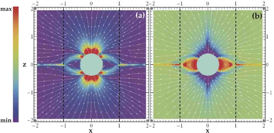
Figure 1: Meridional cross section of the magnetosphere of an aligned (axisymmetric) rotator ($\alpha=0^{o}$). Left panels: meridional electric current density (color plot) and direction (arrows). Right panels: electric charge density (color plot) and meridional magnetic field direction (arrows). Light cylinder shown with dashed lines.

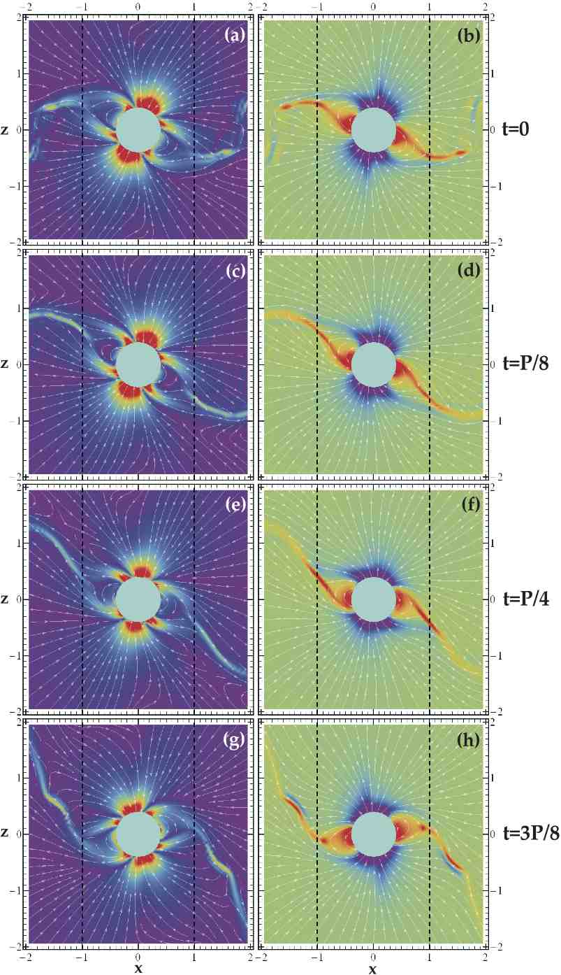
Figure 2: Same as Fig. 1 only for an inclined rotator with $\alpha=30^{o}$ at times $t=0,P/8,P/4,3P/8$. At $t=0$, the magnetic axis lies in the $(x,z)$ plane.

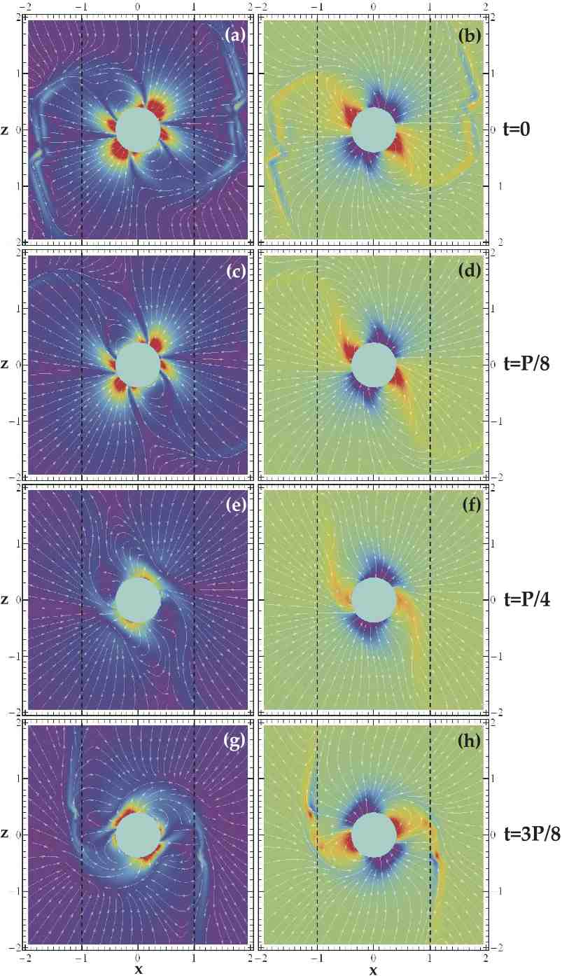
Figure 3: Same as Fig. 2 for $\alpha=60^{o}$.

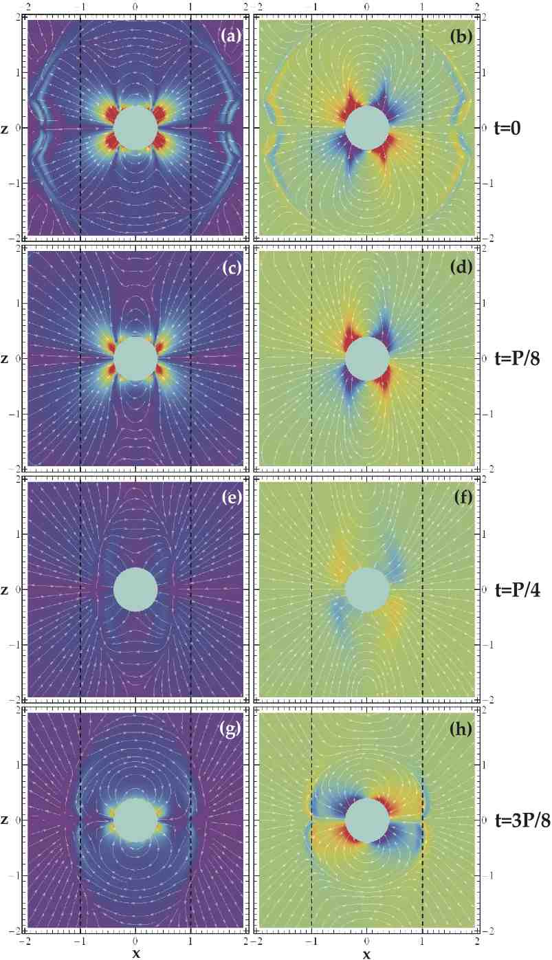
Figure 4: Same as Fig. 2 for $\alpha=90^{o}$.

We have assumed in the past that force-free relativistic ideal MHD is a valid description of the pulsar magnetosphere, except for boundary regions of infinitesimal volume where ideal MHD breaks down and dissipation takes place. Therefore, the magnetospheric electric and magnetic fields ${\bf E}$ and ${\bf B}$ satisfy the three time-dependent Maxwell’s equations in the presence of electric charges $\rho_{e}\equiv(4\pi)^{-1}\nabla\cdot{\bf E}$ and electric currents ${\bf J}$,

$$\frac{\partial{\bf E}}{\partial t}=c\nabla\times{\bf B}-4\pi{\bf J}\ ,$$ (8)

$$\frac{\partial{\bf B}}{\partial t}=-c\nabla\times{\bf E}\ ,$$ (9)

$$\nabla\cdot{\bf B}=0\ ,$$ (10)

as well as the ideal MHD condition

$${\bf E}\cdot{\bf B}=0\ .$$ (11)

As is, the system of equations is degenerate since we need one extra equation for ${\bf J}$. This is provided through the force-free condition

$$\rho_{e}{\bf E}+{\bf J}\times{\bf B}=0\ ,$$ (12)

which, together with eqs. (8)-(11), allows us to express ${\bf J}$ as a function of ${\bf E}$ and ${\bf B}$, namely

$${\bf J}=\frac{c}{4\pi}\nabla\cdot{\bf E}\ \frac{{\bf E}\times{\bf B}}{B^{2}}+\frac{c}{4\pi}\frac{({\bf B}\cdot\nabla\times{\bf B}-{\bf E}\cdot\nabla\times{\bf E})}{B^{2}}\ {\bf B}$$ (13)

(Gruzinov 1999). The first term in eq. (13) corresponds to the Goldreich-Julian charge density moving at the magnetospheric drift velocity $c{\bf E}\times{\bf B}/B^{2}$, whereas the second one corresponds to the extra field-parallel electric current required by the ideal MHD condition that ${\bf E}$ and ${\bf B}$ are everywhere orthogonal (eq. 11). Note that, whenever current/charge sheets appear, they are treated as unresolved MHD discontinuities that satisfy continuity of the Lorentz invariant ${\bf E}^{2}-{\bf B}^{2}$ (our ideal MHD formulation does not capture the non-ideal MHD physical conditions inside a current/charge sheet).

As described in KC09, we start with an initially stationary dipolar magnetic field configuration at a certain inclination angle $\alpha$ (that configuration obviously satisfies the set of equations 8-12), and we then set the central star in rotation. After several stellar rotations (1.5 to 4 depending on the grid numerical diffusivity) the magnetosphere relaxes to a stationary corotating pattern. We produced our own Eulerian solver based on the Yee algorithm (Yee 1966) which we run on a standard PC with 2 Gbyte of RAM. Our computational grid consists of a cubic region with sides 5 times $r_{lc}$ centered around the star, with grid resolution $\delta=0.04r_{lc}$ (we also run a few cases with $\delta=0.025r_{lc}$; see Appendix). In order to reduce computer memory requirements we made use of the central symmetry of the problem and thus integrated only on one half of the above cube. Furthermore, in order to be able to follow the evolution of the magnetosphere for several stellar rotations, we implemented the technique of Perfectly Matched Layers (PML) for our outer boundaries (Berenger 1994, 1996). This technique guarantees non-reflecting and absorbing boundary conditions in vacuum. By applying it to our problem, we showed in practice that this technique also works in non-vacuum relativistic ideal force-free MHD.

Our steady-state results may be summarized in the time sequences of various physical quantities shown on the rotational meridional plane in Figs. (1)-(4) (times in units of one stellar rotation period $P$, with $t=0$ defined as the instance of time when the magnetic axis lies on the plane shown). These are obtained for various inclination angles $\alpha$ after steady state is reached and a stationary corotating electromagnetic field pattern is safely established. Due to the obvious central symmetry of the problem, we plot the time evolution only through one half-period since the pattern repeats itself. On the left panels we plot the distribution of meridional electric current density (the arrows show its direction, and the color plot its magnitude) on a meridional cross section of the magnetosphere. On the right panels we plot the distribution of meridional magnetic field and electric charge density. The toroidal electric current induced by the corotation of the electric charge distributed throughout the dead zone is not reflected in the color diagrams of the left panels.

In the axisymmetric case we obtained a steady-state configuration after about 2.5 stellar rotations (Fig. 1). We recovered the following important characteristics predicted in CKF and others:

1. The dead zone grows up to the light cylinder. Its growth is limited by random reconnection events that occur when its tip accidently crosses the light cylinder. This results in the random generation of outward moving equatorial plasmoids (e.g. Bucciantini et al. 2006).

2. The main magnetospheric poloidal current circuit closes only partially through the two magnetic polar caps. The main part of the return current flows along both surfaces of the separatrix (upper and lower), and connects with an equatorial current sheet at the tip of the dead zone. Interestingly enough, the two surfaces of the separatrix are negatively charged, whereas the equator is positively charged (see eq. 7).

3. The space charge density grows at the tip of the dead zone giving rise to an azimuthal electric current density much stronger than that in the return electric current sheet (C09).

An interesting feature of our numerical method is that the equatorial current sheet is captured well (it is 1-2 computational cells thick) because it coincides with one of our cartesian grid directions. The separatrix current sheet is, however, wider (it is 3-4 computational cells thick). Notice a slight limitation of our numerical scheme: magnetic field lines at high latitudes ($\lower 2.0pt\hbox{$\buildrel{\scriptstyle>}\over{\scriptstyle\sim}$}\ 65^{o}$) reach the boundaries of our computational box before they cross the light cylinder. As a result, the distribution of GJ charge density and CKF electric current are not captured accurately near the rotation axis (see artificial helmet-like enhancements in Fig. 1b; also in Figs. 2b, 3b). Fortunately, the overall effect of that region in the global magnetospheric structure is only minimal.

This simple picture evolves as we move to non-zero inclination angles $\alpha$. In that case we obtained steady-state configurations after about 1.5 stellar rotations (Figs. 2-4). We observed the following characteristic features:

1. The dead zone again grows up to the light cylinder. Random plasmoid formation is again going on beyond the light cylinder (e.g. small knots just outside the light cylinder in Fig. 2g), but is not captured (numerically) as well as in the axisymmetric case (we do see plasmoid formation in the higher resolution simulations shown in Fig. 9 though).

2. As the inclination angle $\alpha$ approaches $90^{o}$, a larger and larger amount of the return current is distributed across the polar cap. An inclination angle of $90^{o}$ is the limit of both an aligned and a counter aligned rotator, and therefore, at $90^{o}$ the two signs of GJ charge and CKF current are expected to be distributed equally across both polar caps, as is seen.

3. A well resolved (numerically) ondulating equatorial current sheet originates at the tip of the dead zone on the light cylinder. This is true even in the orthogonal rotator ($\alpha=90^{o}$). Obviously, the electric circuit cannot close through the dead zone because, in ideal MHD, closed magnetic field lines do not support out/in-flowing electric currents. Therefore, this singular electric current can only be supplied in the form of a current sheet along the separatrix between open and closed field lines. As in the axisymmetric case, electric current sheets inside the light cylinder are not captured well by the numerical simulation (we do resolve parts of the current sheets in Figs. 2c, 2e, 3e, 3g, 9 though). Nevertheless, the observation of strong well resolved (1-2 computational cells wide) electric charge sheets inside the light cylinder (e.g. Figs. 2b, 2d, 2f) and eq. (6) (i.e. the one-to-one relation between charge and current sheets) further support the idea that the singular return currents persist, at least over some part of the separatrix. Interestingly enough, when axisymmetry is broken ($\alpha>0^{o}$), the leading part of the separatrix (that is the surface that faces in the direction of rotation) remains charged negatively, whereas the trailing part is charged positively (we checked that this indeed the case for $\alpha\geq 15^{o}$). On the other hand, the equatorial current sheet remains always charged positively on average.

4. The enhancement of the space charge density at the tip of the dead zone is present in the non-axisymmetric case too, at least over part of the tip (see Figs. 2h, 3h). By analogy to the axisymmetric case, this results in a strong electric current in the return current sheet, both in the azimuthal and outward direction.

5. A novel interesting feature of the numerical solution is that at an azimuthal angle of about $90^{o}$ to that of the magnetic axis, originates a strong source of positive separatrix surface charge (in Fig. 2 notice the strong singular structure that seems to grow on the light cylinder at times $t=P/4$ and is seen moving outward through time $t=P/2$, or equivalently $t=0$). This outflowing positive charge is surrounded by negative charges that guarantee global electric charge conservation. Obviously, any structure observed to move outward in a meridional cross section of the magnetosphere corresponds to a corotating spiral in 3D. We are well aware that a few of the features that we observe in our simulations are due to our numerical resolution (we tested that by running simulations at different resolutions, and found that the details vary slightly; see the Appendix). We observed that this spiral structure survives over several stellar rotations, and therefore, we confirmed that it is steady. In fact, as we will see in the next section, this structure may also leave a signature in the observed pulsar emission.

3 Curvature radiation

As we argued in C09 for an axisymmetric rotator, the tip of the dead zone may play a key role in the pulsar phenomenon. It is impossible to investigate this region in detail in a global magnetospheric numerical simulation. We thus have to rely on an extrapolation of the results in C09 guided by the low resolution numerical simulations of KC09. We believe that, as in the axisymmetric case, the electric charge and electric current density both diverge as the tip of the dead zone approaches the light cylinder. Moreover, the dead zone must end at a short distance from the light cylinder where equipartition is reached between the particle inertia and the magnetic field. At that position, the magnetosphere can only support one type of charge carriers, namely those and only those needed to supply the required GJ density. Therefore, in the current sheet at the tip of the dead zone and beyond, electric charges will move along the direction of the local CKF current ${\bf J}$ with velocities

$${\bf v}=\frac{\bf J}{\rho_{e}}\ .$$ (14)

In analogy to C09, we expect these to correspond to Lorentz factors $10^{5-6}$. The particle trajectories in the current sheet are obviously not straight (at least near the light cylinder), thus the particles will emit curvature radiation along their direction of motion up to a cutoff frequency determined by eq. (4). We note that, in the axisymmetric case where we know analytically the distribution of electric and magnetic fields inside and around the separatrix and the equatorial current sheets (Uzdensky 2003; C09), we are able to calculate in detail the meandering orbits of the particles that support the singular CKF current. These calculations yield a whole spectrum of Lorentz factor values. We therefore expect that the resulting spectrum of curvature radiation is not that of a mono-energetic particle. We plan to investigate this in a forthcoming publication where we will also consider the effect of inverse Compton scattering on soft photons coming from the stellar surface.

We are now in a position to determine the pattern of emitted curvature radiation, both its light curve and polarization profile, for various pulsar inclination and observation angles. The local radiation intensity is weighted by a) the Goldreich-Julian number density, b) the inverse square of the particle instantaneous radius of curvature, and c) the fourth power of the particle Lorentz factor $\gamma$ (for acceleration perpendicular to the direction of motion; Jackson 1975). The simulation provides the distribution of electric charge density $\rho_{e}$, and the characteristic elements of the particle orbits in the observer’s inertial frame through eq. (14) (direction, radius of curvature), but is not good enough to yield accurately the Lorentz factor $\gamma$. We will thus assume simply that positrons/electrons attain a very large limiting Lorentz factor ($\gamma\sim 10^{6}$) at the tip of the separatrix and in the equatorial current sheet. In practice, we implement the following numerical procedure:

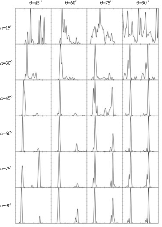
Figure 5: High-energy light curves obtained for various inclination and observation angles $\alpha$ and $\theta$. Horizontal axes are normalized to the period of one stellar rotation, with zeros corresponding to the arrival of the radio pulse (see text). Vertical axes are normalized to the maximum pulse intensity.

1. We identify the regions of the magnetosphere where the particle velocities $\bf v$ (as given by eq. 14) are larger than $0.9c$. We also require that the particle density $\left|\rho_{e}\right|$ be above a certain value in order to avoid regions with fictitiously high values of $\bf v$. This selection indeed coincides with the ondulating equatorial current sheet outside the light cylinder.

2. We assume that every point in the selected region emits in a forward small opening angle ($2^{o}-5^{o}$) around its instantaneous direction of motion.

3. The local curvature radiation intensity is weighted proportionally to the local particle density $|\rho_{e}|$ and inversely proportionally to the square of the local radius of curvature of particle orbits. There is no weighting with $\gamma^{4}$ since, as we said, $\gamma$ is set to the same large value in the equatorial current sheet.

4. We select the direction of observation and add up the contributions along that direction from every point in the region selected in (1) and (2) weighted as in (3) during one full pulsar rotation. In doing so, we take into account the light-crossing time-delay from the various parts of the magnetosphere.

The light curves produced by curvature radiation in the equatorial current sheet from the tip of the dead zone on the light cylinder and beyond are shown in Fig. (5). We plot pulse profiles with intensities normalized to the maximum pulse intensity for various inclination and observation angles $\alpha$ and $\theta$ (calculated with respect to the axis of rotation). In the context of our model of equatorial current sheet emission, emission intensity dramatically decreases at high latitudes, and the quality of our numerical results deteriorates. This is why we only plot light curves for $\theta\geq 45^{o}$. Azimuthal phase zero is defined as the phase where a photon that is emitted radially outward from the surface of the star when the magnetic axis lies in the plane defined by the rotation axis and the line of sight reaches the observer. As defined, azimuthal phase zero corresponds to the arrival phase of the radio pulse in the prevailing model of pulsar radio emission coming from a magnetospheric region just above the magnetic polar cap. Several interesting features in the pulse/sub-pulse distribution are worth mentioning:

1. Pulses are narrower when observed from higher latitudes.

2. Pulses are narrow despite the fact that the corresponding emission regions have significant azimuthal extent. This effect is analogous to the ‘caustics’ obtained in pulsar slot-gap models for radiation emitted along trailing magnetic field lines (e.g. Arons 1983; Harding et al. 2008).

3. Interpulse intensity decreases fast compared to that of the main pulse as the observer moves away from the rotational equatorial plane.

4. Whenever an interpulse is seen ($\alpha$ greater than about $30^{o}$), pulse-interpulse separation varies mostly between about 0.4 to 0.5 times the period (Fig. 6). The closer the inclination or the observation angle is to $90^{o}$, the closer the pulse-interpulse separation is to one-half of the period.

5. The main pulse trails the radio pulse (in the prevailing model of radio pulsar emission coming from above the stellar polar cap) by about 0.15 to 0.25 times the period whenever an interpulse is seen, and up to one-half of the period when no interpulse is seen. In particular, notice the striking similarity between our Fig. (6) and Fig. 4 of Abdo et al. (2009).

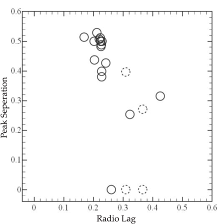
Figure 6: Phase difference between the high-energy peaks, versus phase lag between the radio and main high-energy peak. Dotted circles correspond to those cases where interpulses are not clearly defined.

We would like to end this section with an investigation of the expected polarization angle profiles. Radiation propagates in the magnetosphere in the form of ordinary and extraordinary wave modes (Barnard & Arons 1986). The ordinary mode is polarized in the plane of the wave vector and the local magnetic field direction, whereas the extraordinary mode is linearly polarized perpendicularly to the wave vector and the local magnetic field. Gil, Lyubarsky & Melikidze (2004) showed that, for radiation frequencies $\nu\leq\nu_{lim}$, the ordinary mode is heavily suppressed, and only the extraordinary mode escapes freely and thus reaches the observer. In our case $\nu_{c}\approx\nu_{lim}$ in the emission region (eq. 5), and therefore, we will heretofore consider only the radiation mode linearly polarized perpendicularly to the line of sight and the local magnetic field.

In Fig. (7) we show the polarization profiles that correspond to the light curves in Fig. (5). The polarization angles shown are the mean polarization angles from all the emission points observed at each time instance weighted by their relative intensity. They lie in the range $-90^{o}$ to $+90^{o}$ and are measured on the plane of the sky with zero along the projected direction of the axis of rotation, and positive in the north-to-east direction. Our results are not very clear because of numerical problems associated with the equatorial current sheet. We do observe several cases with dramatic (up to $\pm 90^{o}$) polarization angle sweeps across the main pulses and interpulses. In particular, at observation angles $\theta=60^{o}$ and $75^{o}$, we obtain polarization angle sweeps reminiscent of those seen in the Crab pulsar (e.g. Słowikiwska et al. 2009). In order to explore the origin of this effect, we plot in Fig. (8) the polarization angles expected from radiation produced in $2\pi$ annular regions around the rotation axis if one happens to be looking along the direction of the local ${\bf J}$. The observed polarization angles sweeps are associated with the abrupt change of magnetic field direction at the crossings of the equatorial current sheet. We thus conclude that, in the context of our model, polarization angle sweeps essentially cut across and resolve the thin equatorial current sheet, as in the phenomenological model of Petri & Kirk 2005.

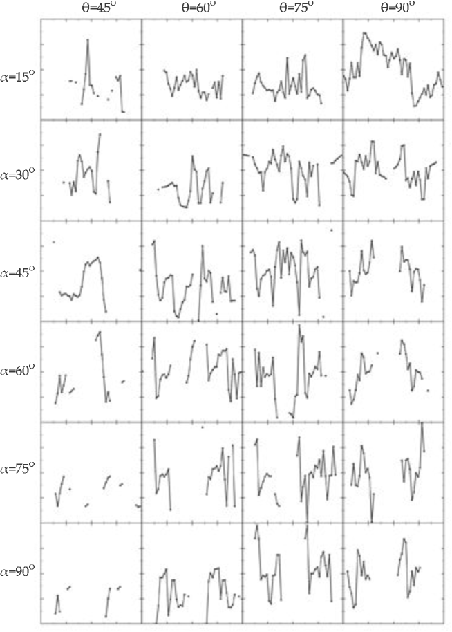
Figure 7: High-energy polarization angle profiles obtained for various inclination angles $\alpha$ and various observation angles $\theta$. Horizontal scale as in Fig. 5. Vertical scale from $-90^{o}$ to $+90^{o}$.

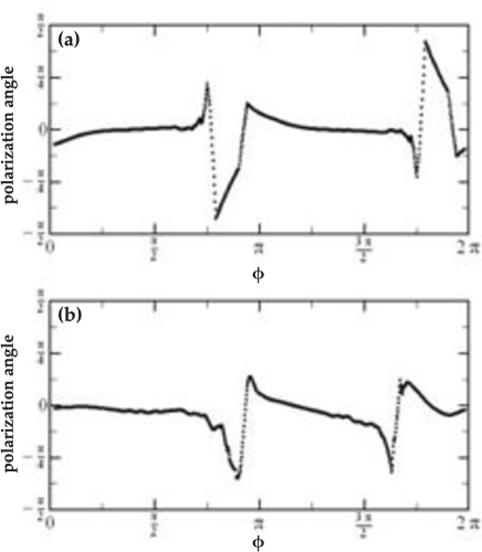
Figure 8: Expected polarization angles from curvature radiation produced in two annular regions at positions $r\sin\theta=1.5r_{lc}$, $r\cos\theta=0$ and $0.5r_{lc}$ (a and b respectively) as a function of azimuthal angle $\phi$ for an inclined rotator with $\alpha=50^{o}$.

4 Summary

2D and 3D numerical simulations of the force-free relativistic pulsar magnetosphere show that a strong electric current develops at the tip of the closed line region on the light cylinder. This electric current consists of extremely relativistic electrons and positrons that move along curved trajectories in the azimuthal and outward direction in an equatorial current sheet beyond the light cylinder. As in C09, we call this configuration the pulsar synchrotron.

In the present paper, we studied the emission of curvature radiation from the pulsar synchrotron, and defered the study of inverse Compton to a future publication. We showed that curvature radiation seems to be responsible for the high-energy pulsed emission up to X-ray frequencies in normal pulsars, and up to $\gamma$-ray frequencies in millisecond pulsars. We produced high-energy light curves that show sharp pulses and interpulses in pulsars with high inclination angles $\alpha\ \lower 2.0pt\hbox{$\buildrel{\scriptstyle>}\over{\scriptstyle\sim}$}\ 45^{o}$, and wide single pulses in pulsars with low inclination angles $\alpha\ \lower 2.0pt\hbox{$\buildrel{\scriptstyle<}\over{\scriptstyle\sim}$}\ 30^{o}$ (except when observed from very low latitudes with respect to the rotation equatorial plane). Our model of an extended emission region in the equatorial direction is in some sense complimentary to that of the polar cap ‘lighthouse beam’ emission. Polarization angle profiles are less well determined numerically. They do show, however, abrupt polarization angle sweeps that are associated with the abrupt change of direction of the magnetic field as we cut across the equatorial current sheet.

Our conclusions are based on our preliminary numerical simulations of the 3D force-free relativistic pulsar magnetosphere. In particular, we focus our investigation on the most difficult part of our simulation, the return-current sheet. This may explain certain strange features in our compilation of light curves (e.g. for $\theta=45^{o}$, $\alpha=15^{o}$ and $75^{o}$), and the abrupt changes in the polarization angle profiles. On the other hand, some of these features may be attributed to the newly discovered equatorial spiral structure that originates at $90^{o}$ from the magnetic axes on the tip of the closed-line region on the light cylinder. A deeper investigation of the equatorial return-current sheet will have to wait our forthcoming supercomputer numerical simulations (expected improvement in the numerical resolution by a factor of 5 to 10).

Regarding the expected lag between the radio and high-energy pulses, our results compare well with newly available data from NASA’s Fermi $\gamma$-ray space telescope (Abdo et al. 2009). This comparison assumes that radio emission is coming from a small height above the stellar magnetic polar cap. Interestingly enough, radio emission from Vela is on average polarized in a direction perpendicular to the axis of rotation (assumed to coincide with the elongation axis of the nebula). This is consistent with the observed pulsar radio emission consisting mainly of extraordinary waves produced by relativistic electrons and positrons that move along open dipolar magnetic field lines above the polar cap (e.g. Lai, Chernoff & Cordes 2001; Gil, Lyubarsky & Melikidze 2004). On the other hand, high-energy (optical) emission from Vela is on average polarized along the rotation axis as predicted by our model (Mignani et al. 2007; Fig. 8). This picture does not apply in the case of the Crab pulsar where pulses are emitted in phase and are on average polarized along the axis of rotation at all wavelengths (from radio to $\gamma$-rays; Słowikowska et al. 2009). We can thus argue that, in that particular case, radio emission may just be the low-energy part of the observed high-energy curvature radiation emission amplified by coherence effects, as proposed in C09. It would thus be worthwhile to search for a radio component in phase and with the same polarization as the high-energy one in the Fermi pulsars too. If such component is not discovered, it would be interesting to study why radio coherence from the pulsar synchrotron is suppressed in most (but not all) pulsars.

Appendix A Numerical resolution

In order to investigate the influence of the numerical grid resolution $\delta$ on our results, we compared two simulations for an inclined rotator with $\alpha=50^{o}$, one with our standard grid resolution $\delta=0.04r_{lc}$, and one obtained with higher resolution $\delta=0.025r_{lc}$ (Fig. 9).

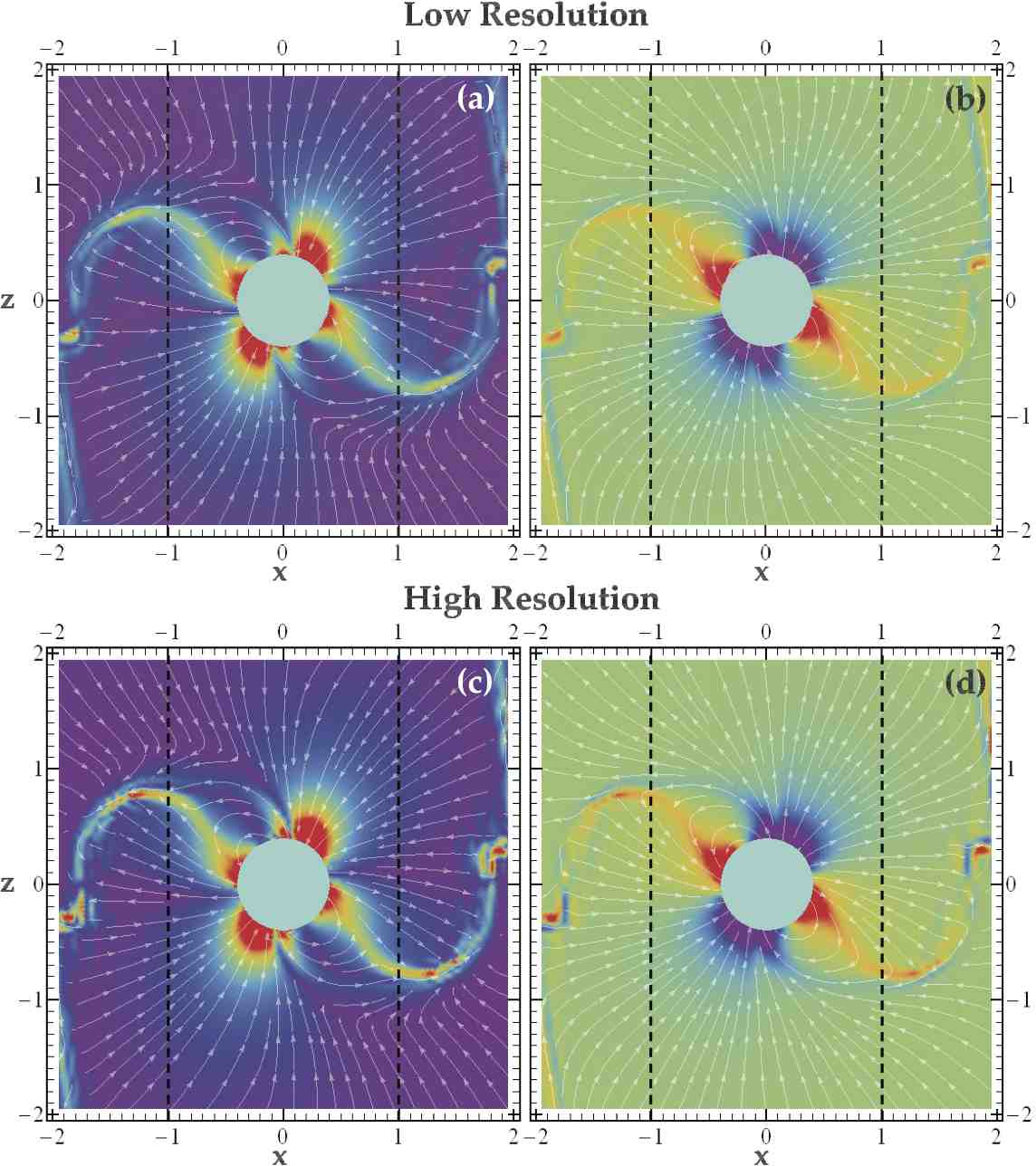
Figure 9: Comparison between our standard $\delta=0.04r_{lc}$ and a higher $\delta=0.025r_{lc}$ grid resolutions. Same as Fig. 2 for $\alpha=50^{o}$ and $t=0$.

In the latter we obtain the same overall magnetic field distribution, only it is sharper. In particular:

1. We better resolved random plasmoid formation outside the light cylinder.

2. We obtained a sharper (1-2 computational cells wide) return current structure along the positively charged part of the separatrix. This supports our conclusion that the singular return current sheet discovered in CKF survives also in the inclined rotator.

3. The positively charged spiral feature outside the light cylinder mentioned in § 2 is also present. This supports our view that it is indeed a real feature of the magnetosphere.

References

- (1) Abdo, A. A. et al. 2009, submitted (arXiv:0910.1608)
- (2) Arons, J. 1983, ApJ, 266, 215
- (3) Bai, X.-N. & Spitkovsky, A. 2009, submitted (arXiv:0910.5741)
- (4) Barnard, J. J. & Arons, J. 1986, ApJ, 302, 138
- (5) Bartel N., 1978, A& A, 62, 393
- (6) Bucciantini, N., Thompson, T. A., Arons, J., Quataert, E. & Del Zanna, L. 2006, MNRAS, 368, 1717
- (7) Berenger, J.-P. 1994, Journal of Comp. Phys., 114, 185
- (8) Berenger, J.-P. 1996, Journal of Comp. Phys., 127, 363
- (9) Contopoulos, I., Kazanas, D. & Fendt, C. 1999, ApJ, 511, 351 (CKF)
- (10) Contopoulos, I. 2005, A& A, 442, 579
- (11) Contopoulos, I. 2009, MNRAS, 396L, 6
- (12) Cordes J. M., 1981, in Sieber W., Wielebinski R., eds, Pulsars: 13 years of research on neutron stars, Proceedings of the Symposium, 115, Dordrecht, Bonn
- (13) Daugherty, J. K. & Harding, A. K. 1982, ApJ, 252, 337
- (14) Ferguson D. C., 1981, in Sieber W., Wielebinski R., eds, Pulsars: 13 years of research on neutron stars, Proceedings of the Symposium, 141, Dordrecht, Bonn
- (15) Gil, J., Lyubarsky, Y. & Melikidze, G. I. 2004, ApJ, 600, 872
- (16) Gold T., 1968, Nat, 218, 731
- (17) Gold T., 1969, Nat, 221, 25
- (18) Goldreich, P. & Julian, W. H. 1969, ApJ, 157, 869
- (19) Gruzinov, A. 1999, astro-ph/9902288
- (20) Gruzinov, A. 2005, Phys. Rev. Lett., 94, 021101
- (21) Harding, A. K., Stern, J. V., Dyks, J. & Frackowiak, M. 2008, ApJ, 680, 1378
- (22) Jackson, J. D. 1975, Classical Electrodynamics (New York: Wiley)
- (23) Kalapotharakos, C. & Contopoulos, I. 2009, A& A, 496, 495 (KC09)
- (24) Lai, D., Chernoff, D. F. & Cordes, J. M. 2001, ApJ, 549, 1111
- Michel (2005) Michel, F. C. 2005, The Texas-Mexico Conf. on Astroph. eds. S. Torres-Peimbert & G. MacAlpine, RevMexAA, 23, 27
- MB (08) Mignani, R. P., Bagnulo, S., Dyks, J., Lo Curto, G. & Słowikowska, A. 2008, A& A, 467, 1157
- (27) Petri, J. & Kirk, J. G. 2005, ApJ, 627L, 37
- (28) Radhakrishnan, V. & Cooke, D. J. 1969, ApL, 3, 225
- (29) Ruderman, M. A. & Sutherland, P. G. 1975, ApJ, 196, 51
- (30) Słowikowska, A., Kanbach, G., Kramer, M. Stefanescu, A. 2009, MNRAS,397, 103
- (31) Spitkovsky, A. 2006, ApJ, 648, L51
- (32) Sturrock, P. A., 1971, ApJ, 164, 529
- (33) Timokhin, A. N., 2006, MNRAS, 368, 1055
- (34) Uzdensky, D. 2003, ApJ, 598, 446
- (35) Yee, K. 1966, IEEE Trans. Antennas Propagat., 14, 302