Nanoscopic spontaneous motion of liquid trains: non-equilibrium molecular dynamics simulation

Abstract

Macroscale experiments show that a train of two immiscible liquid drops, a bislug, can spontaneously move in a capillary tube because of surface tension asymmetries. We use molecular dynamics simulation of Lennard-Jones fluids to demonstrate this phenomenon for NVT ensembles in sub-micron tubes. We deliberately tune the strength of intermolecular forces and control the velocity of bislug in different wetting and viscosity conditions. We compute the velocity profile of particles across the tube, and explain the origin of deviations from the classical parabolae. We show that the self-generated molecular flow resembles the Poiseuille law when the ratio of the tube radius to its length is less than a critical value.

I Introduction

Dynamics of liquid flow in nanoscopic systems has received great attention in recent years. Design and manufacturing of nanofluidic devices, fluid transport phenomenon WHI07 ; TCC02 , the recent development of “lab-on-a-chip” technology C06 ; MEvdB05 and fluid imbibition in the nanopores of biomembranes, are amongst notable applications. Our knowledge, however, has been mostly confined to the dynamics of capillary flows at macroscales Wash21 ; Yang04 where the relationships between the velocity and contact angle with the surface tension, dynamic viscosity and wetting characteristics are known Gen85 ; Chan05 .

Generating and controlling the driving force of liquids in extremely thin tubes is a major technological challenge, which suggests the application of self-propelling systems. The spontaneous motion of liquid drops was initially reported by Marangoni Mar71 and it was shown to occur in variably wet and temperature controlled tubes Wei97 ; MH00 , chemically reacting fluids deG98 ; BBM94 ; DdSO95 and in surface-tension-driven motions Bic00 . In all these cases the driving force comes from physical or environmental asymmetries, which may cause a net motion. In the present study, we are interested in the surface-tension-driven motion of droplets because of its importance in microfluidic automation Chan05 ; Squ05 . In particular, we intend to scale down (by several orders of magnitude) a self-propelling liquid system, called a bislug, which was introduced by Bico & Quéré Bic00 ; Bic02 . Although the motion of a bislug is fairly explained by the dynamics of Newtonian fluids in macroscales, there is neither theoretical nor experimental evidence for the applicability/validity of the same physical rules for molecular ensembles at sub-micron scales.

A liquid bislug is composed of two liquid droplets, liquid I and liquid II, juxtaposed inside a capillary tube and bounded by a third fluid (fluid III) on both sides (Fig. 1a). The system therefore involves three interfaces each called a meniscus. The difference between adhesive interactions of two neighboring fluids directly determines the meniscus wetting power, and so its contact angle. In the partial wetting state, the contact angle is finite, and it reduces to zero in the limit of complete wetting condition. Moreover, the cohesive interactions inside each of two adjacent fluids as well as adhesive interactions between them, determine the meniscus surface tension. The total driving force exerted on a bislug is

$$F\propto\gamma_{d}=\gamma_{1}\cos\theta_{1}+\gamma_{12}\cos\theta_{12}-\gamma_{2}\cos\theta_{2},$$ (1)

where $\gamma_{d}$ is the effective surface tension, and the parameters ($\gamma_{1},\gamma_{12},\gamma_{2}$) and ($\theta_{1},\theta_{12},\theta_{2}$) are, respectively, the surface tensions and contact angles (Fig. 1a).

(a)

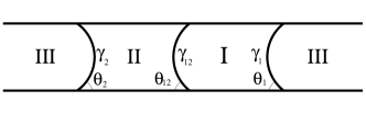
(b)

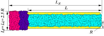
Figure 1: (a) Configuration of a liquid bislug in a nanotube. (b) Initial state of our LJ fluids. Fluid III initially fills the tube and liquids I and II occupy the reservoir.

In macroscale experiments, when all menisci partially wet the tube wall, the contact angles are changed so that the forces at three menisci compensate each other and keep the liquid bislug in static equilibrium Yang04 ; Bic02 . As soon as at least one of the menisci completely wets the tube, its contact angle drops to zero and the existing force balance breaks down. If liquid II is more wetting than liquid I (see Fig. 1a), it will be deposited on the tube wall while liquid I moves with a constant velocity. In this article, we carry out a molecular dynamics simulation of a nanoscopic system of immiscible liquids, and reveal its self-propelling dynamics for a wide range of material and interfacial properties.

II Model Description

We use the setup of Fig. 1b to incrementally turn on the force contribution of each meniscus. Using fluid III, we simulate the presence of air or any other fluid and equalize its pressure at both sides of the bislug using periodic boundary conditions. Fluid III also suppresses possible diffusion effects. We consider a cylindrical tube of the length $L$ and radius $R$ composed of fixed solid particles that do not interact with each other. The wall particles are distributed on a cylindrical arrangement with a constant distance of $\sigma$, which is our length scale. This is how we build a rigid impenetrable wall. The tube is attached to a $(L_{x}-L)\times L_{y}\times L_{z}(L_{y}=L_{z}=2.5R)$ boxy reservoir on the left side. The height (and also width) of the reservoir is larger than the tube diameter, and the joint between the tube and the reservoir is rigid. We apply periodic boundary conditions at the lateral walls of the reservoir (perpendicular to the view shown in Fig. 1b) as well as in the longitudinal direction: all liquid particles may freely enter the reservoir if they reach to the rightmost boundary of the tube.

There are four different types of particles corresponding to liquid I, liquid II, fluid III, and the solid wall, which are numbered in our subsequent formulation as 1, 2, 3, and 4, respectively. Fluid particles are located initially at a cubic lattice with the lattice constant of $\sigma$, and all particles interact through the Lennard-Jones (LJ) potential

$$U_{ij}(r)=4\epsilon_{ij}\left[\left(\frac{\sigma_{ij}}{r}\right)^{12}-\beta_{ij}\left(\frac{\sigma_{ij}}{r}\right)^{6}\right].$$ (2)

Here $\epsilon_{ij}$ and $\sigma_{ij}$ define the strength and effective range of $U_{ij}$ between the particles of types $i$ and $j$. Theoretically, the radius of influence of the LJ potential extends to infinity and all binary interactions will involve non-zero finite forces. Nevertheless, the computational cost will be drastically decreased if one cuts off the attractive LJ force for radii above some $r_{c}$. For all interactions, we choose $r_{c}=2.5\sigma$, which has already been used in the literature Mar02 ; DMB07 ; DMB08 and it guarantees a drop of the attractive force below $2\%$ of its maximum value. The choice of $r_{c}=2.5\sigma$ has also resulted in a reasonable match between molecular dynamics simulations and experimental data Rao76 . We control the mixing of different fluids by setting Her05

$$\beta_{ij}=\left\{\begin{array}[]{ccc}1&{\rm if}&i=j,\\ 0.1&{\rm if}&i\not=j,\\ \end{array}\right.$$ (3)

for $i,j=1,2,3$.

The surface tension at each interface depends on the internal interactions of each fluid as well as interactions between two fluids, controlled by $\epsilon_{ij}$ ($i,j=1,2,3$). The wetting power of each liquid depends on adhesive interactions between the liquid and tube particles, which is solely controlled by $\epsilon_{i4}$ in the LJ potential. The difference between the values of $\epsilon_{i4}/\epsilon_{ii}$ for adjacent fluids, determines the contact angle of their interface (meniscus) such that the concave part faces towards the fluid with lower $\epsilon_{i4}/\epsilon_{ii}$. The resultant driving force $F$ is controlled by adjusting the values of $\epsilon_{ij}$ and so the contact angles DMB07 ; DMB08 . Moreover, the viscosity of the $i$th fluid, $\eta_{i}$, is determined by $\epsilon_{ii}$.

We implement non-equilibrium molecular dynamics simulation of an NVT ensemble Allen87 using the velocity Verlet algorithm with the integration time step $\delta t=0.005t_{0}$ where

$$t_{0}=\sqrt{\frac{m\sigma^{2}}{48k_{\rm B}T}}=\frac{1}{\sqrt{38.4}}.$$ (4)

The chosen time step corresponds to $10^{-14}$ seconds for a wide range of fluids, and its efficiency has already been confirmed in the study of liquid argon Fre02 ; Allen87 . We use the dimensionless values of $\sigma=1$, the particle mass $m=1$, and set $k_{\rm B}T=0.8$. To preserve the ensemble temperature at a constant value, a Nosé-Hoover thermostat hoover85 is applied at each step. We scale all lengths and velocities by $\sigma$ and $\sigma/t_{0}$, respectively.

III Simulation Results

We do our simulations when: (A) all fluids have the same viscosity $\eta$ and surface tension $\gamma$ (B) viscosities of fluids differ from each other. We then generate the normalized displacement $x/L_{x}$ of the front meniscus (FM) versus the normalized time $t/t_{0}$ for different values of $\alpha=R/L$. The position of the front meniscus $x$ is measured from the leftmost boundary of the reservoir, and it is defined as the location where the density of liquid I reaches to $90\%$ of its maximum value. Although the experiments of type A are unrealistic, they help us to independently investigate the influence of contact angles on the bislug dynamics. We study three possible circumstances: (i) only the rear meniscus (between liquid II and fluid III) completely wets the tube (ii) the rear and middle menisci completely wet the tube (iii) all three menisci completely wet the tube. We use two tubes of radii $R=10.34$ and $5.17$.

III.1 Equal Viscosities

We set $\epsilon_{11}$=$\epsilon_{22}$=$\epsilon_{33}$=1 to create equal viscosities, and use $\epsilon_{34}=0.5$ and $\epsilon_{12}$=$\epsilon_{23}$=$\epsilon_{13}$=1 to get the same boundary interactions between different fluids. The internal interactions of each fluid is governed by $\beta_{ii}$=1 ($i$=1,2,3) and we set $\beta_{12}$=$\beta_{23}$=$\beta_{13}$=0.1 Her05 to prevent liquids from mixing. We start our computations with a case that all menisci partially wet the tube. The contact angles in a partial wetting condition lie in the range $0<\theta_{1},\theta_{12},\theta_{2}<90^{\circ}$ should one choose the values of $0.5\leq\epsilon_{14},\epsilon_{24}\leq 1.1$. In such a circumstance, the capillary force pulls both liquids into the tube subsequently, while fluid III leaves the tube and enters the reservoir.

As each meniscus enters the tube, the driving force is altered and the slope of the displacement curve of the FM varies accordingly. One can therefore identify three phases on displacement curves (Fig. 2). The first phase begins when liquid I enters the tube and it ends when liquid II flows into the tube. The driving force of the first phase is proportional to $\gamma_{d}=\gamma\cos\theta_{1}$. The second phase starts by the inflow of liquid II and continues until the last molecules of liquid II leave the reservoir. This stage involves two active menisci implying $\gamma_{d}=\gamma(\cos\theta_{1}+\cos\theta_{12})$. In the third (and last) phase, the whole bislug is inside the tube and the driving force is computed from Eq. (1).

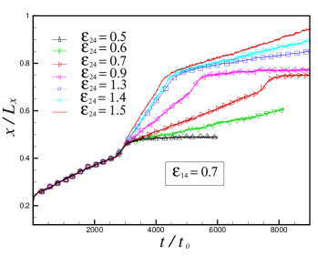
Figure 2: The normalized displacement curve of the front meniscus ($x/L_{x}$) versus time in partial and complete wetting conditions with $\alpha=0.107(R=10.34,L=96.14)$ and $\eta_{1}=\eta_{2}=\eta_{3}$.

Fig. 2 displays the displacement history of the FM for several values of $0.5\leq\epsilon_{24}\leq 0.9$ and for $\epsilon_{14}=0.7$. By keeping $\epsilon_{14}$ constant, we have fixed the driving force of the FM. For the three cases $\epsilon_{24}$=$0.5$, $0.6$, and $0.7$ that satisfy $\epsilon_{24}\leq\epsilon_{14}=0.7$, the concave side of the middle meniscus (between liquids I and II) faces liquid II ($\theta_{12}\geq 90^{\circ}$) and it resists the driving force of FM. Consequently, in the second phase the bislug moves slower than the first one. For $\epsilon_{24}=0.5$ we have $\epsilon_{24}$= $\epsilon_{34}$, whose natural implication is $\epsilon_{14}-\epsilon_{24}$= $\epsilon_{14}-\epsilon_{34}$, which in turn leads to the condition $\theta_{12}+\theta_{1}=180^{\circ}$. This says that the surface tension of the front meniscus cancels that of the middle one, and the bislug must stop as soon as liquid I leaves the reservoir (zero velocity in the second part of displacement curve in Fig. 2a). By increasing $\epsilon_{24}$, the velocity of FM increases as long as liquid II has not completed its entrance into the tube. However, after the complete drainage of liquid II from the reservoir, the displacement curve of the FM becomes flat indicating a static equilibrium in partial wetting conditions: $\gamma(\cos\theta_{1}+\cos\theta_{12}-\cos\theta_{2})=0$.

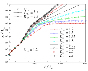
Figure 3: The normalized displacement curve of the front meniscus ($x/L_{x}$) versus time in partial and complete wetting conditions with $\alpha=0.107$ ($R$=10.34, $L$=96.14) and $\eta_{1}=\eta_{2}=\eta_{3}$.

For $\epsilon_{24}\geq 1.2$ and with the same $\epsilon_{14}=0.7$, the rear meniscus completely wets the tube, and results in $\theta_{2}=0$ and $F\propto\gamma_{d}=\gamma(\cos\theta_{1}+\cos\theta_{12}-1)$. This is the first complete wetting situation, which holds over the range $1.2\leq\epsilon_{24}<1.5$. Since $\cos\theta_{1}+\cos\theta_{12}>1$, the bislug undergoes a sustained motion after entering the tube until liquid II is totally consumed, or the FM reaches the end of the tube (Fig. 2). By further increasing $\epsilon_{24}$, we obtain a critical value of $\epsilon_{24}\approx 1.5$ beyond which the middle meniscus completely wets the tube. This is the second complete wetting state ($\theta_{2}=\theta_{12}=0$) and the force components corresponding to $\gamma\cos\theta_{2}$ and $\gamma\cos\theta_{12}$ cancel each other identically. The bislug is thus driven by the FM: $F\propto\gamma_{d}=\gamma\cos\theta_{1}$. Fig. 4 shows a snapshot of the moving bislug in its third phase. It is evident that liquid II leaves a thin stationary layer on the tube wall.

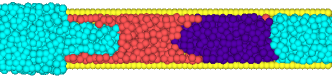
Figure 4: A moving bislug corresponding to the case of $\epsilon_{14}$=$0.7$ and $\epsilon_{24}$=1.5 in Fig. 2.

To obtain the state of complete wetting condition for all three menisci, we fix $\epsilon_{14}=1.2$ and carry out new simulations (see Fig. 3). For the very special case of $\epsilon_{14}=\epsilon_{24}=1.2$ that implies $\theta_{1}=\theta_{2}=0$ and $\theta_{12}=90^{\circ}$, and according to our assumption $\gamma$=$\gamma_{1}$=$\gamma_{12}$=$\gamma_{2}$, liquids I and II will behave as a single droplet, which is pulled into the tube by the maximum force $F_{\rm I}\propto\gamma$ exerted by the FM, but it stops once the rear meniscus enters the tube and contributes $F_{\rm II}\propto-\gamma$ to the total driving force. We then increase $\epsilon_{24}$ so that the force components $\gamma\cos\theta_{1}$ and $\gamma\cos\theta_{2}$ cancel each other and the driving force comes from the middle meniscus whose concave side faces liquid I for $\epsilon_{24}>\epsilon_{14}$. The middle meniscus, however, will be in partial wetting as long as $\cos\theta_{12}<1$. Therefore, the velocity of the FM (and so the bislug) is boosted by increasing $\epsilon_{24}$ because $\cos\theta_{12}\propto\epsilon_{24}-\epsilon_{14}$. The four last graphs of Fig. 3 show that the velocity of the FM is saturated for $\epsilon_{24}>2.8$, which corresponds to the complete wetting condition of all menisci.

The experiments with $(\epsilon_{14},\epsilon_{24})=0.7$ in Fig. 2 and $(\epsilon_{14},\epsilon_{24})=1.2$ in Fig. 3 show that the bislug velocity in the second phase is slightly less than the first phase while the equality of $\epsilon_{14}$ and $\epsilon_{24}$ should have resulted in $\theta_{12}=90^{\circ}$ and identical velocities during the first and second phases of motion. Our explanation of this phenomenon is as follows: while the middle meniscus is driven, it is subject to back-and-forth oscillations that alternately change the contact angle and keep its average magnitude larger than the expected value (this is because the particles near the contact point of a meniscus usually lag the field particles, which feel less frictional force). For the special case of $\epsilon_{14}=\epsilon_{24}$, the average value of $\theta_{12}$ marginally exceeds $90^{\circ}$ and causes a tiny resistive force. Therefore, the velocity of the bislug is slightly reduced during the second phase. So far we have considered different cases of bislug motion when three fluids have the same viscosity $\eta$. Below we vary the viscosities of fluids and investigate realistic cases.

III.2 Different Viscosities

We use Kirkwood-Buff’s expression

$$\gamma=\int dx\left\{p_{xx}(x)-\frac{1}{2}\left[p_{yy}(x)+p_{zz}(x)\right]\right\},$$ (5)

and compute the surface tension $\gamma$ from the elements of pressure tensor using the equilibrium molecular dynamics simulation of two adjacent, thermostated liquids in a cube Kirk49 . In similar conditions, we apply the Green-Kubo integral to obtain the viscosity of our LJ fluids Allen87 ; RW82 . The element $p_{xx}(x)$ of the pressure tensor is normal to the interface. For the system of fluids with equal viscosities and surface tensions, we find $\gamma=2.6\pm 0.15$ and $\eta=3.25\pm 0.25$. It is remarked that the application of other methods such as shear flow, gives compatible results BLHL05 .

We now vary the viscosities of fluids around $\eta\approx 3.25$. Increasing the value of $\epsilon_{ii}$ enables us to increase the viscosity of the $i$th fluid, $\eta_{i}$. By taking $\epsilon_{34}=0.1$ and $\epsilon_{ii}$=$(0.5,0.8,1,1.1,1.2)$, we find

$$\eta_{i}=(1.6\!\pm\!0.1,2.6\!\pm\!0.2,3.25\!\pm\!0.25,3.6\!\pm\!0.32,4.\!\pm\!0.33),$$ (6)

and apply our NVT code to compute $x(t)/L_{x}$ when $\eta_{1}>3.25>\eta_{2}>\eta_{3}=1.6$. Some of our results are displayed in Fig. 5. As one could anticipate, the first two phases of displacement curves are no longer linear versus time, and the profile of the first phase resembles a parabolic pattern $x/L_{x}\propto\sqrt{t/t_{0}}$, which is the well-known Washburn equation DMB07 . It is evident that even for the case of different viscosities, the third phase of each displacement curve has still a constant velocity in accordance with macroscale experiments Bic00 .

By comparing the results of Figures 2 and 5 we conclude that reducing $\eta_{3}$ (with respect to $\eta_{1}$ and $\eta_{2}$) boosts the bislug velocity considerably. It is remarked that we needed to decrease $\epsilon_{34}$ while we were doing so for $\epsilon_{33}$ just to preserve the wetting condition of the FM. In Fig. 5, comparing the graphs of $(\epsilon_{11},\epsilon_{22})=(1,0.8)$ and $(\epsilon_{11},\epsilon_{22})=(1,1)$ suggests that decreasing $\eta_{2}$ (while $\eta_{1}$ is kept constant) induces an even faster motion because the deposition of liquid II on the tube wall speeds up. The graphs corresponding to $\epsilon_{22}=0.8$ show that the bislug velocity is slowed down by increasing $\epsilon_{11}$, which means higher values of $\eta_{1}$ and therefore a larger viscous force. This effect is clearly evident from the longer first phase (similar to $\sqrt{t/t_{0}}$) of the bislug displacement curve.

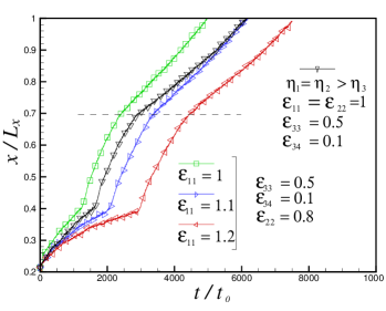
Figure 5: The normalized displacement curve of the front meniscus ($x/L_{x}$) versus time for $\alpha=0.107$ ($R$=10.34, $L$=96.14), $(\epsilon_{14},\epsilon_{24})=(0.7,2.3)$ and different viscosities $\eta_{1}>\eta_{2}>\eta_{3}$. Here, the FM is in partial wetting condition and the other two menisci completely wet the tube wall. We demonstrate the special case of $\eta_{1}$=$\eta_{2}>\eta_{3}$ to show the effect of $\eta_{1}$ and $\eta_{2}$ on the bislug velocity independently. Horizontal dashed line approximately indicates the beginning of the third phase.

IV Physics of the Flow

In all cases, the velocity of the FM, $V(t)=dx/dt$, is constant over the last phase of displacement curves, and it is proportional to $\gamma_{d}$. The motion with a constant $V$ is due to the balance between the driving force $F=2\pi R\gamma_{d}$ and the viscous friction force $F_{\rm drag}$ from the tube wall. i.e., $F-F_{\rm drag}=mdV/dt=0$ where $m$ is the total mass inside the tube. When all fluids have the same viscosity $\eta$ and the flow is Poiseuille, one obtains

$$V\equiv V_{p}=\frac{\gamma_{d}\alpha}{4\eta},~{}~{}F_{\rm drag}=8\pi\eta LV_{p}.$$ (7)

In this equation, $\eta$ and $L$ must be replaced, respectively, with $\eta_{1}=\eta_{2}$ and the bislug length when fluid III has a negligible contribution to the dynamics. Given $\alpha=R/L$, the magnitude of $V_{p}$ can therefore be calculated. To see in which conditions the bislug velocity attains the value of $V_{p}$, we carry out some new calculations with the two radii $R=5.17$ and $10.34$, and by taking several tube lengths of $52.51\leq L\leq 96.14$, which yield $0.107\leq\alpha\leq 0.197$. We use fluids of the same viscosity, set $\epsilon_{14}=1.2$, and let all menisci completely wet the tube wall. Some of our results have been illustrated in Fig. 6. According to our simulations, the quantity $V/L_{x}$ tends to $V_{p}/L_{x}$ by decreasing $\alpha$ and the relative error $|V-V_{p}|/V_{p}$ reduces from $33\%$ (for $\alpha=0.197$) to $3\%$ (for $\alpha=0.107$). In the complete wetting condition of all menisci and for $\epsilon_{24}=3.5$, we find the critical value $\alpha_{\rm cr}\approx 0.1$ below which the velocity of the FM becomes identical to $V_{p}$. A couple of our experiments correspond to $R=5.17$ and $L=96.14$ that give $\alpha=0.053$. With such a small ratio and for $\epsilon_{14}=\epsilon_{24}=1.2$, liquids I and II remain separated but they behave as a single drop. For the stronger wall interactions of liquid II with $\epsilon_{24}=3.5$, the relative velocity error further decreases and we obtain $V\approx V_{p}$. This is evident from Fig. 6 as the first and third phases of motion have the same slope.

We are using a Nosé-Hoover thermostat, which is mainly applied to equilibrium phenomena. The self-propelling motion of liquid trains, however, is a non-equilibrium case and a thermostat may destroy the Galilean invariance of dynamical equations. Through computing the Washburn prefactor, we show that such an effect is quite small in most of our simulations that correspond to narrow tubes of $\alpha\leq\alpha_{cr}$. When fluids I and III are immiscible and have the same viscosity, the time dependence of the displacement function $x/L_{x}$ is linear during the entrance of liquid I into the tube, and the Washburn equation $V\sim t^{-1/2}$ is transformed to the ordinary law of capillary dynamics: $V=\gamma\alpha\cos\theta/(4\eta)$. This becomes $V=0.2\alpha$ for ($\gamma,\eta$)=($2.6,3.25$) in our setup and in the complete wetting condition of the FM ($\theta=\theta_{1}=0$). For $\epsilon_{14}=1.2$ and $\alpha=0.107$, the first phase of the displacement curves in Fig. 3 corresponds to the complete wetting of the FM and the slope of this phase gives $V\approx 0.0225$. On the other hand, the capillary equation yields $V=0.2\times 0.107=0.0214$. For the case with $(R,\alpha)=(5.17,0.053)$ and $\epsilon_{14}=\epsilon_{24}=1.2$ in Fig. 6, the capillary equation leads to $V=0.2\times 0.053=0.0106$ while the slope of the first phase of the displacement curve is $V\approx 0.0108$. The relative errors between theoretical predictions and our simulations are therefore $5\%$ and $1.8\%$ for $\alpha=0.107$ and $\alpha=0.053$, respectively. This result shows that the effect of the Nosé-Hoover thermostat on the Galilean invariance of governing equations is insignificant, specially when $\alpha<\alpha_{cr}$.

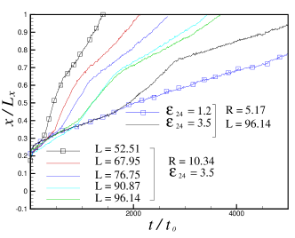
Figure 6: The normalized displacement curve of the front meniscus ($x/L_{x}$) versus $t/t_{0}$ for $0.107\leq\alpha\leq 0.197$ with $R=10.34$, and for $\alpha=0.053$ with $R=5.17$. All menisci are in complete wetting condition, and we have set $\epsilon_{14}=1.2$ and $\eta_{1}=\eta_{2}>\eta_{3}$.

Let $v(\zeta,r,t)$ denote the longitudinal velocity of molecules inside the tube where $r$ and $\zeta$ are the distances of molecules from the tube centerline and the reservoir outlet, respectively, and $t$ is the time. Small circles and squares in Fig. 7 display the simulated profile of

$$\bar{v}(r)=\lim_{t\rightarrow\infty}\frac{1}{t}\int_{0}^{t}dt\frac{1}{L}\int_{L_{x}-L}^{L_{x}}v(\zeta,r,t)d\zeta,$$ (8)

together with the best-fitted parabolic curves to the data. These data have been obtained for the case with $(\epsilon_{14},\epsilon_{24})$=$(0.7,1.5)$ in Fig. 2, and $(\epsilon_{11},\epsilon_{22})$=$(1,0.8)$ in Fig. 5. The time average in equation (8) is computed only over the third phase of bislug motion, and averaging along the tube length helps us to reduce the noise of dynamic capillary waves and work with a better statistical data. It is seen that for $\alpha=0.107$, the flow inside the tube is almost Newtonian and laminar. There is a better match between the simulated data and the best-fitted parabolic curve near the wall because the boundary layer (due to shearing) initially develops near the wall and then penetrates into inner regions. In other words, molecules near the tube centerline are subject to radial motions more than those living near the wall. Our numerical experiments show that the functional form of $\bar{v}(r)$ does not depend on the contact angle $\theta_{12}$ but on $\alpha$. By increasing $\alpha$, the gradient $\frac{d}{dr}\bar{v}(r)$ increases near the wall, enhances $F_{\rm drag}$ and we get $V<V_{p}$. The existence of $\alpha_{\rm cr}$ has also been confirmed by the macroscale experiments of Bico & Quéré Bic02 . They report $\alpha_{\rm cr}\approx 0.07$ and ascribe the drop of velocity for $\alpha>\alpha_{\rm cr}$ to the viscous dissipation at the menisci. Below, we argue that the physical mechanism of the process is different in molecular ensembles.

The information of any developing phenomenon, like meniscus oscillation and boundary layer formation, is transmitted by individual molecules that interact by their neighbors and after several “kicks” lose their initial memory. The oscillations of driving menisci remain unseen for downstream particles when the tube length is increased: for a long bislug, the number of longitudinal interactions between molecules is quite large and the coming information from oscillating menisci is gradually dissolved. What actually matters in the radial direction is the development of the boundary layer whose propagation into central regions is again through interactions between molecules. When the tube radius is small, the number of radially disturbing kicks that molecules experience is small and the boundary layer can fully extend to the tube centerline. In tubes of larger radii, however, molecules undergo too many radial interactions (kicks) and lose the “shearing information” that they had to carry to molecules near the tube centerline. As a result, the boundary layer is not fully developed and some amount of the kinetic energy is carried by radial motions. An evidence for this process is the flattening of the profile of $\bar{v}(r)$ in central regions (see Fig. 7). To have a Poiseuille flow in sub-micron scales, we thus need both a small radius (measured in units of $\sigma$) and a large tube length. These would mean the existence of some $\alpha_{\rm cr}$, which should correlate with the relaxation time of the bislug.

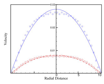
Figure 7: The profile of $\bar{v}(r)$ versus the radial distance $r$ from the tube centerline. Circles correspond to the case of equal viscosities with $(\epsilon_{14},\epsilon_{24})=(0.7,1.5)$ in Fig. 2. Squares show the profile of the case with $(\epsilon_{11},\epsilon_{22})=(1,0.8)$ in Fig. 5 (for different viscosities). Solid and dashed lines are the best-fitted parabolic curves.

V Conclusions

The bislug motion is a consequence of the transfer of free energy, from initially separated liquids, to the longitudinal component of the kinetic energy of molecules. The system chooses a definite direction of motion because the different wetting capabilities of liquids I and II breaks the symmetry along the tube axis. Independent of the viscosities of fluids, we observed a constant bislug velocity when both liquids I and II leave the reservoir. The Washburn law governs the history of $x(t/t_{0})/L_{x}$ in the entrance phase of liquid I to the tube DMB07 . The bislug will not move (the first four cases in Fig. 2) when the adhesion with the wall is not enough for making a permanent and stable binding between all molecules of a component (either of liquids I and II) and the tube wall.

We showed that the spontaneous motion of immiscible liquids inside the tubes of sub-micron radii is an efficient process in certain wetting conditions, and it leads to significant mass transport should one use appropriate liquids. An external pressure gradient has played a decisive role in previous experiments M05TM09 and simulations TMc09 of water flow in carbon nanotubes. Our fundamental achievement was to capture the flow characteristics of a nanoscopic self-propelling system in the absence of an external pressure field. The size of the bislug, which indeed determines the relaxation time, and its relation with the form of the velocity profile across a small tube, helped us to suggest a new physical mechanism for explaining the deviations from the Poiseuille law. Our results have potential applications in mass transport in fluidic devices and also in the separation of immiscible liquids in sub-micron scales.

VI Acknowledgments

We thank the referees for their constructive comments, which helped us to improve the presentation of our simulations. This work was partially supported by the research vice-presidency at Sharif University of Technology.

References

- (1) M. Whitby and N. Quirke, Nature Nanotechnology 2, 87 (2007).
- (2) S.W.P. Turner, M. Cabodi, and H.G. Craighead, Phys. Rev. Lett. 88, 128103 (2002).
- (3) H. Craighead, Nature 442, 387 (2006).
- (4) D. Mijatovic, J.C.T. Eijkel, and A. van den Berg, Lab on a Chip 5, 492 (2005).
- (5) E.W. Washburn, Phys. Rev. 17, 273 (1921).
- (6) L.J. Yang, T.J. Yao, and Y. Tai, J. Micromech. Microeng. 14, 220 (2004).
- (7) P.G. de Gennes, Rev. Mod. Phys. 57, 827 (1985).
- (8) W.K. Chan, and C. Yang, J. Micromech. Microeng. 15, 1722 (2005).
- (9) C. Marangoni, Ann. Phys. Chem. 143, 337 (1871).
- (10) M.M. Weislogel, AIChE J. 43, 645 (1997).
- (11) V. Mazouchi and G.M. Homsy, Phys. Fluids 12, 542 (2000).
- (12) P.G. de Gennes, Physica A 249, 196 (1998).
- (13) C. Bain, G. Burnett-Hall, and R. Montgomerie, Nature 372, 414 (1994).
- (14) F. Domingues dos Santos and T. Ondarcuh, Phys. Rev. Lett. 75, 2972 (1995).
- (15) J. Bico and D. Quéré, Europhys. Lett. 51, 546 (2000).
- (16) T.M. Squires and S.R. Quake, Rev. Mod. Phys. 77, 977 (2005).
- (17) J. Bico and D. Quéré, J. Fluid Mech. 467, 101 (2002).
- (18) G. Matric, F. Genter, D. Seveno, D. Coulon and J. De Coninck, Langmuir. 18, 7971 (2002).
- (19) D.I. Dimitrov, A. Milchev, and K. Binder, Phys. Rev. Lett. 99, 054501 (2007).
- (20) D.I. Dimitrov, A. Milchev, and K. Binder, Langmuir 24, 1232 (2008).
- (21) M. Rao, and D. Levesque, J. Chem. Phys. 65, 3233 (1976).
- (22) E. Diaz-Herrera, J. Alejandre, J. Ramirez-Santiago, and F. Forstmann, J. Chem. Phys. 110, 8084 (1999).
- (23) M.P. Allen, and D.J. Tildesley, Computer Simulation of Liquids (Clarendon Press, Oxford, 1987).
- (24) D. Frenkle and B. Smit, Understanding Molecular Simulation, From Algorithm to Applications (Academic Press, 2002).
- (25) W.G. Hoover, Phys. Rev. A 31, 1695 (1985).
- (26) J.G. Kirkwood and F.P. Buff, J. Chem. Phys. 17, 338 (1949).
- (27) J.S. Rowlinson and B. Widom, Molecular Theory of Capillarity (Clarendon, Oxford, 1982).
- (28) J.A. Backer, C.P. Lowen, H.C.J. Hoefsloot, and P.D. Ledema, J. Chem. Phys. 122, 154503 (2005).
- (29) M. Majumder, N. Chopra1, R. Andrews, and B.J. Hinds, Nature 438, 44 (2005)
- (30) J.A. Thomas and A.J.H. McGaughey, Phys. Rev. Lett. 102, 184502 (2009).