Cluster synchronization in networks of coupled non-identical dynamical systems

Abstract

In this paper, we study cluster synchronization in networks of coupled non-identical dynamical systems. The vertices in the same cluster have the same dynamics of uncoupled node system but the uncoupled node systems in different clusters are different. We present conditions guaranteeing cluster synchronization and investigate the relation between cluster synchronization and the unweighted graph topology. We indicate that two condition play key roles for cluster synchronization: the common inter-cluster coupling condition and the intra-cluster communication. From the latter one, we interpret the two well-known cluster synchronization schemes: self-organization and driving, by whether the edges of communication paths lie at inter- or intra-cluster. By this way, we classify clusters according to whether the set of edges inter- or intra-cluster edges are removable if wanting to keep the communication between pairs of vertices in the same cluster. Also, we propose adaptive feedback algorithms on the weights of the underlying graph, which can synchronize any bi-directed networks satisfying the two conditions above. We also give several numerical examples to illustrate the theoretical results.

Cluster synchronization is considered to be more momentous than complete synchronization in brain science and engineering control, ecological science and communication engineering, social science and distributed computation. Most of the existing works only focused on networks with either special topologies such as regular lattices or coupled two/three groups. For the general coupled dynamical systems, theoretical analysis to clarify the relationship between the (unweighted) graph topology and the cluster scheme, including both self-organization and driving, is absent. In this paper, we study this topic and find two essential conditions for an unweighted graph topology to realize cluster synchronization: the common inter-cluster coupling condition and the intra-cluster communication. Thus under these conditions, we present two manners of weighting to achieve cluster synchronization. One is adding positive weights on each edges with keeping the invariance of the cluster synchronization manifold and the other is an adaptive feedback weighting algorithms. We prove the availability of each manner. From these results, we give an interpretation of the two clustering synchronization schemes: self-organization and driving, involved with the unweighted graph topology, via the communication between pairs of individuals in the same cluster. Thus, we present one way to classify the clusters via whether the set of inter- or intra-cluster edges are removable if still wanting to keep the communication between vertices in the same cluster.

I Introduction

Recent decades witnesses that chaos synchronization in complex networks has attracted increasing interests from many research and application fields Pik ; Boc1 ; Wang1 , since it was firstly introduced in Ref. Yamada . Word “synchronization” comes from Greek, which means “share time” and today, it comes to be considered as “time coherence of different processes”. Many new synchronization phenomena appear in a wide range of real systems, such as biology Str , neural networks Gra , physiological processes Gla . Among them, the most interesting cases are complete synchronization, cluster synchronization, phase synchronization, imperfect synchronization, lag synchronization, and almost synchronization etc. See Ref. Boc and the references therein.

Complete synchronization is the most special one and characterized by that all oscillators approach to a uniform dynamical behavior. In this situation, powerful mathematical techniques from dynamical systems and graph theory can be utilized. Pecora et.al. Pec proposed the Master Stability Function for transverse stability analysis Ash of the diagonal synchronization manifold. This method has been widely used to study local completer synchronization in networks of coupled system Loc_syn . Refs. Wu ; Glo_syn ; Lu proposed a framework of Lyapunov function method to investigate global synchronization in complex networks. One of the most important issues is how the graph topology affects the synchronous motion Boc1 . As pointed out in Ref. Wu2 , the connectivity of the graph plays a significant role for chaos synchronization.

Cluster synchronization is considered to be more momentous in brain science Sch and engineering control Clu_con , ecological science Clu_eco and communication engineering Clu_com , social science Sto and distributed computation Clu_dis . This phenomenon is observed when the oscillators in networks are divided into several groups, called clusters, by the way that all individuals in the same cluster reach complete synchronization but the motions in different clusters do not coincide. Cluster synchronization of coupled identical systems are studied in Refs. Bel1 ; Liu ; Wei ; Jalan . Among them, Jalan et. al. Jalan pointed out two basic formations which realize cluster synchronization. One is self-organization, which leads to cluster with dominant intra-cluster couplings, and the other is driving, which leads to cluster with dominant inter-cluster couplings.

Nowadays, the interest of cluster synchronization is shifting to networks of coupled non-identical dynamical systems. In this case, cluster synchronization is obtained via two aspects: the oscillators in the same cluster have the same uncoupled node dynamics and the inter- or intra-cluster interactions realize cluster synchronization via driving or/and self-organizing configurations. Refs. Liu proposed cluster synchronization scheme via dominant intra-couplings and common inter-cluster couplings. Ref. Sor studied local cluster synchronization for bipartite systems, where no intra-cluster couplings (driving scheme) exist. Refs. ChenL investigated global cluster synchronization in networks of two clusters with inter- and intra-cluster couplings. Belykh et. al. studied this problem in 1D and 2D lattices of coupled identical dynamical systems in Ref. Bel1 and non-identical dynamical systems in Ref. Bel2 , where the oscillators are coupled via inter- or/and intra-cluster manners. Ref. Pha used nonlinear contraction theory Loh to build up a sufficient condition for the stability of certain invariant subspace, which can be utilized to analyze cluster synchronization (concurrent synchronization is called in that literature). However, up till now, there are no works revealing the relationship between the (unweighted) graph topology and the cluster scheme, including both self-organization and driving, for general coupled dynamical systems.

The purpose of this paper is to study cluster synchronization in networks of coupled non-identical dynamical systems with various graph topologies. In Section 2, we formulate this problem and study the existence of the cluster synchronization manifold. Then, we give one way to set positive weights on each edges and derive a criterion for cluster synchronization. This criterion implies that the communicability between each pair of individuals in the same cluster is essential for cluster synchronization. Thus, we interpret the two communication schemes: self-organization and driving, according to the communication scheme among individuals in the same cluster. By this way, we classify clusters according to the manner by which synchronization in a cluster realizes. In Sec. 3, we propose an adaptive feedback algorithms on weights of the graph to achieve a given clustering. In Sec. 5, we discuss the cluster synchronizability of a graph with respect to a given clustering and present the general results for cluster synchronization in networks with general positive weights. We conclude this paper in Sec. 6.

II Cluster synchronization analysis

In this section, we study cluster synchronization in a network with weighted bi-directed graph and a given division of clusters. We impose the constraints on graph topology to guarantee the invariance of the corresponding cluster synchronization manifold and derive the conditions for this invariant manifold to be globally asymptotically stable by the Lyapunov function method. Before that, we should formulate the problem.

Throughout the paper, we denote a positive definite matrix $Z$ by $Z>0$ and similarly for $Z<0$, $Z\leq 0$, and $Z\geq 0$. We say that a matrix $Z$ is positive definite on a linear subspace $V$ if $u^{\top}Zu>0$ for all $u\in V$ and $u\neq 0$, denoted by $Z|_{V}>0$. Similarly, we can define $Z|_{V}<0$, $Z|_{V}\geq 0$, and $Z|_{V}\leq 0$. If a matrix $Z$ has all eigenvalues real, then we denote by $\lambda_{k}(Z)$ the $k$-th largest eigenvalues of $Z$. $Z^{\top}$ denotes the transpose of the matrix $Z$ and $Z^{s}=(Z+Z^{\top})/2$ denotes the symmetry part of a square matrix $Z$. $\#A$ denotes the number of the set $A$ with finite elements.

II.1 Model description and existence of invariant cluster synchronization manifold

A bi-directed unweighted graph $\mathcal{G}$ is denoted by a double set $\{\mathcal{V},\mathcal{E}\}$, where $\mathcal{V}$ is the vertex set numbered by $\{1,\cdots,m\}$, and $\mathcal{E}$ denotes the edge set with $e(i,j)\in\mathcal{E}$ if and only if there is an edge connecting vertices $j$ and $i$. $\mathcal{N}(i)=\{j\in\mathcal{V}:~{}e(i,j)\in\mathcal{E}\}$ denotes the neighborhood set of vertex $i$. The graph considered in this paper is always supposed to be simple (without self-loops and multiple edges) and bi-directed. A clustering $\mathcal{C}$ is a disjoint division of the vertex set $\mathcal{V}$: $\mathcal{C}=\{\mathcal{C}_{1},\mathcal{C}_{2},\cdots,\mathcal{C}_{K}\}$ satisfying (i). $\bigcup_{k=1}^{K}\mathcal{C}_{k}=\mathcal{V}$; (ii). $\mathcal{C}_{k}\bigcap\mathcal{C}_{l}=\emptyset$ holds for $k\neq l$.

The network of coupled dynamical system is defined on the graph $\mathcal{G}$. The individual uncoupled system on the vertex $i$ is denoted by an $n$-dimensional ordinary differential equation $\dot{x}^{i}=f_{k}(x^{i})$ for all $i\in\mathcal{C}_{k}$, where $x^{i}=[x^{i}_{1},\cdots,x^{i}_{n}]^{\top}$ is the state variable vector on vertex $i$ and $f_{k}(\cdot):\mathbb{R}^{n}\to\mathbb{R}^{n}$ is a continuous vector-valued function. Each vertex in the same cluster has the same individual node dynamics. The interaction among vertices is denoted by linear diffusion terms. It should be emphasized that $f_{k}$ for different clusters are distinct, which can guarantee that the trajectories are apparently distinguishing when cluster synchronization is reached.

Consider the following model of networks of linearly coupled dynamical system IEEE :

$$\dot{x}^{i}=f_{k}(x^{i})+\sum_{j\in\mathcal{N}(i)}w_{ij}\Gamma(x^{j}-x^{i}),~{}i\in\mathcal{C}_{k},~{}k=1,\cdots,K.$$ (1)

where $w_{ij}$ is the coupling weight at the edge from vertex $j$ to $i$ and $\Gamma=[\gamma_{uv}]_{u,v=1}^{n}$ denotes the inner connection by the way that $\gamma_{uv}\neq 0$ if the the $u$-th component of the vertices can be influenced by the $v$-th component. The graph $\mathcal{G}$ is bi-directed and the weights are not requested to be symmetric. Namely, we don’t request $w_{ij}=w_{ji}$ for each pair $(i,j)$ with $e(i,j)\in\mathcal{E}$.

Let $A=[a_{ij}]_{i,j=1}^{m}$ be the adjacent matrix of the graph $\mathcal{G}$. That is, $a_{ij}=1$ if $e(i,j)\in\mathcal{E}$; $a_{ij}=0$ otherwise. Then, model (1) can be rewritten as

$$\dot{x}^{i}=f_{k}(x^{i})+\sum_{j=1}^{m}a_{ij}w_{ij}\Gamma(x^{j}-x^{i}),~{}i\in\mathcal{C}_{k},~{}k=1,\cdots,K.$$ (2)

In this paper, cluster synchronization is defined as follows:

1. The differences among trajectories of vertices in the same cluster converge to zero as time goes to infinity, i.e.,

   $$\lim_{t\to\infty}[x^{i}(t)-x^{j}(t)]=0,~{}\forall~{}i,j\in\mathcal{C}_{k},~{}k=1,\cdots,K;$$ (3)

2. The differences among the trajectories of vertices in different clusters do not converge to zero, i.e., $\overline{\lim}_{t\to\infty}|x^{i^{\prime}}(t)-x^{j^{\prime}}(t)|>0$ holds for each $i^{\prime}\in\mathcal{C}_{k}$ and $j^{\prime}\in\mathcal{C}_{l}$ with $k\neq l$.

As mentioned above, we suppose that the latter one can be guaranteed by the incoincidence of $f_{k}(\cdot)$. Under this prerequisite assumption, cluster synchronization is equivalent to the asymptotical stability of the following cluster synchronization manifold with respect to the clustering $\mathcal{C}$:

$$\mathcal{S}_{\mathcal{C}}(n)=\{[{x^{1}}^{\top},\cdots,{x^{m}}^{\top}]^{\top}:~{}x^{i}=x^{j}\in\mathbb{R}^{n},~{}\forall~{}i,j\in\mathcal{C}_{k},~{}k=1,\cdots,K\}.$$ (4)

To investigate cluster synchronization, a prerequisite requirement is that the manifold $\mathcal{S}_{\mathcal{C}}(n)$ should be invariant through Eqs. (2). Assume that $x^{i}(t)=s^{k}(t)$ for each $i\in\mathcal{C}_{k}$ is the synchronized solution of the cluster $\mathcal{C}_{k}$, $k=1,\cdots,K$. By Eqs. (2), each $s^{k}$ must satisfy

$$\dot{s}^{k}=f_{k}(s^{k})+\sum_{k^{\prime}=1,k^{\prime}\neq k}^{K}\alpha_{i,k^{\prime}}\Gamma(s^{k^{\prime}}-s^{k}),~{}~{}\forall~{}i\in\mathcal{C}_{k},$$ (5)

where $\alpha_{i,k^{\prime}}=\sum_{j\in\mathcal{C}_{k^{\prime}}}a_{ij}w_{ij}$. This demands $\alpha_{i_{1},k^{\prime}}=\alpha_{i_{2},k^{\prime}}$ for any $i_{1}\in\mathcal{C}_{k}$, $i_{2}\in\mathcal{C}_{k}$, namely, $\alpha_{i,k^{\prime}}$ is independent of $i$. Therefore, we have

$$\alpha_{i,k^{\prime}}=\alpha(k,k^{\prime}),~{}i\in\mathcal{C}_{k},~{}k\neq k^{\prime}.$$ (6)

This condition is sufficient and necessary for the cluster synchronization manifold $\mathcal{S}_{\mathcal{C}}(n)$ is invariant through the coupled system (2) for general maps $f_{k}(\cdot)$.

Denote $\mathcal{N}_{k^{\prime}}(i)=\mathcal{N}(i)\bigcap\mathcal{C}_{k^{\prime}}$, and define an index set $\mathcal{L}^{i}_{k}=\{k^{\prime}:~{}k^{\prime}\neq k,~{}{\rm and}~{}N_{k^{\prime}}(i)\neq\emptyset\}$. The set $\mathcal{L}^{i}_{k}$ represents those clusters other than $\mathcal{C}_{k}$ and have links to the vertex $i$. To satisfy the condition (6), the following common inter-cluster coupling condition over the unweighted graph topology should be satisfied: for $k=1,\cdots,K$,

$$\mathcal{L}^{i}_{k}=\mathcal{L}^{i^{\prime}}_{k},~{}\forall~{}i,i^{\prime}\in\mathcal{C}_{k}.$$ (7)

Therefore, we can use $\mathcal{L}_{k}$ to represent $\mathcal{L}_{k}^{i}$ for all $i\in\mathcal{C}_{k}$ if the common inter-cluster coupling condition is satisfied.

Throughout this paper, we assume that the vector-valued function $f_{k}(x)-\alpha\Gamma x:\mathbb{R}^{n}\to\mathbb{R}^{n}$ satisfies decreasing condition for some $\alpha\in\mathbb{R}$. That is, there exists $\delta>0$ such that

$$(\xi-\zeta)^{\top}\bigg{[}f_{k}(\xi)-f_{k}(\zeta)-\alpha\Gamma(\xi-\zeta)\bigg{]}\leq-\delta(\xi-\zeta)^{\top}(\xi-\zeta).$$ (8)

holds for all $\xi,\zeta\in\mathbb{R}^{n}$. This condition holds for any globally Lipschitz continuous function $f(\cdot)$ for sufficiently large $\alpha>0$ and $\Gamma=I_{n}$. However, even though $f(\cdot)$ is only locally Lipschitz, if the solution of the coupled system (1) is essentially bounded, then restricted to such bounded region, the condition (8) also holds for sufficiently large $\alpha$ and $\Gamma=I_{n}$. In this paper, we suppose that the solution of the coupled system (2) is essentially bounded.

II.2 Cluster synchronization analysis

In the following, we investigate cluster synchronization of networks of coupled non-identical dynamical systems withe the following weighting scheme:

$$w_{ij}=\left\{\begin{array}[]{ll}\frac{c}{d_{i,k}}&j\in\mathcal{N}_{k}(i)~{}{\rm and}~{}\mathcal{N}_{k}(i)\in\emptyset\\ 0&{\rm otherwise},\end{array}\right.$$ (11)

where $d_{i,k^{\prime}}=\#\mathcal{N}_{k}(i)$ denotes the number of elements in $N_{k^{\prime}}(i)$ and $c$ denotes the coupling strength.. Thus, the coupled system becomes:

$$\dot{x}^{i}=f_{k}(x^{i})+c\bigg{[}\sum_{\mathcal{N}_{k^{\prime}}(i)\neq\emptyset}\frac{1}{d_{i,k^{\prime}}}\sum_{j\in\mathcal{N}_{k^{\prime}}(i)}\Gamma(x^{j}-x^{i})\bigg{]},~{}i\in\mathcal{C}_{k},~{}k=1,\cdots,K.$$ (12)

It can be seen that in Eqs. (12), for each $i\in\mathcal{C}_{k}$, the corresponding $\alpha_{i,k^{\prime}}=c$ for all $k^{\prime}\in\mathcal{L}_{k}$ under the common inter-cluster coupling condition. The general situation can be handled by the same approach and will be presented in the discussion section.

We denote the weighted Laplacian of the graph as follows. For each pair $(i,j)$ with $i\neq j$, $l_{ij}=\frac{1}{d_{i,k}}$ if $j\in\mathcal{N}_{k}(i)$ and $\mathcal{N}_{k}(i)\neq\emptyset$ for some $k\in\{1,\cdots,K\}$, and $l_{ij}=0$ otherwise; $l_{ii}=-\sum_{j=1}^{m}l_{ij}$. Thus, Eqs. (12) can be rewritten as:

$$\dot{x}^{i}=f_{k}(x^{i})+c\sum_{j=1}^{m}l_{ij}\Gamma x^{j},~{}i\in\mathcal{C}_{k},~{}k=1,\cdots,K.$$ (13)

The approach to analyze cluster synchronization is extended from that used in Ref. Lu to study complete synchronization. Let $d=[d_{1},\cdots,d_{m}]^{\top}$ be a vector with $d_{i}>0$ for all $i=1,\cdots,m$. We use the vector $d$ to construct a (skew) projection of $x=[{x^{1}}^{\top},\cdots,{x^{m}}^{\top}]^{\top}$ onto the cluster synchronization manifold $\mathcal{S}_{\mathcal{C}}(n)$. Define an average state with respect to $d$ in the cluster $\mathcal{C}_{k}$ as

$$\bar{x}^{k}_{d}=\frac{1}{\sum_{i\in\mathcal{C}_{k}}d_{i}}\sum_{i\in\mathcal{C}_{k}}d_{i}x^{i}.$$

Thus, we denote the projection of $x$ on the cluster synchronization manifold $\mathcal{S}_{\mathcal{C}}(n)$ with respect to $d$ as: $\bar{x}_{d}=[\tilde{x}^{1^{\top}},\cdots,\tilde{x}^{m^{\top}}]^{\top}$ is denoted as:

$$\tilde{x}^{i}=\bar{x}_{d}^{k},~{}if~{}i\in\mathcal{C}_{k}.$$

Then, the variations $x^{i}-\bar{x}^{k}_{d}$ compose the transverse space:

$$\mathcal{T}_{\mathcal{C}}^{d}(n)=\bigg{\{}u=[{u^{1}}^{\top},\cdots,{u^{m}}^{\top}]^{\top}\in\mathbb{R}^{mn}:~{}u^{i}\in\mathbb{R}^{n},~{}\sum_{i\in\mathcal{C}_{k}}d_{i}u^{i}=0,~{}\forall~{}k=1,\cdots,K\bigg{\}}.$$

In particular, in the case of $n=1$, it denotes

$$\mathcal{T}_{\mathcal{C}}^{d}(1)=\bigg{\{}u=[u^{1},\cdots,u^{m}]^{\top}\in\mathbb{R}^{m}:~{}\sum_{i\in\mathcal{C}_{k}}d_{i}u^{i}=0,~{}\forall~{}k=1,\cdots,K\bigg{\}}.$$

From the definition, we have the following lemma which is repeatedly used below.

Lemma 1

For each $k\in 1,\cdots,K$, it holds

$$\sum_{i\in\mathcal{C}_{k}}d_{i}(x^{i}-\bar{x}_{d}^{k})=0.$$

In fact, note

$$\sum_{i\in\mathcal{C}_{k}}d_{i}(x^{i}-\bar{x}_{d}^{k})=\sum_{i\in\mathcal{C}_{k}}d_{i}x^{i}-\sum_{i\in\mathcal{C}_{k}}d_{i}\bigg{(}\frac{1}{\sum_{j\in\mathcal{C}_{k}}d_{j}}\bigg{)}\sum_{i^{\prime}\in\mathcal{C}_{k}}d_{i^{\prime}}x^{i^{\prime}}=\sum_{i\in\mathcal{C}_{k}}d_{i}x^{i}-\sum_{i^{\prime}\in\mathcal{C}_{k}}d_{i^{\prime}}x^{i^{\prime}}=0.$$

The lemma immediately follows. As a direct consequence, we have

$$\sum_{i\in\mathcal{C}_{k}}d_{i}(x^{i}-\bar{x}_{d}^{k})^{\top}J_{k}=\bigg{[}\sum_{i\in\mathcal{C}_{k}}d_{i}(x^{i}-\bar{x}_{d}^{k})\bigg{]}^{\top}J_{k}=0$$

for any $J_{k}$, with a proper dimension, independent of the index $i$.

Since the dimension of $\mathcal{T}_{\mathcal{C}}^{d}(n)$ is $n(m-K)$, the dimension of $\mathcal{S}_{\mathcal{C}}$ is $nK$, and $\mathcal{S}_{\mathcal{C}}(n)$ is disjoint with $\mathcal{T}_{\mathcal{C}}^{d}(n)$ except the origin, $\mathbb{R}^{mn}=\mathcal{S}_{\mathcal{C}}(n)\bigoplus\mathcal{T}_{\mathcal{C}}^{d}(n)$, where $\bigoplus$ denotes the direct sum of linear subspaces. With these notations, the cluster synchronization is equivalent to the transverse stability of the cluster synchronization manifold $\mathcal{S}_{\mathcal{C}}(n)$, i.e., the projection of $x$ on the transverse space $\mathcal{T}_{\mathcal{C}}^{d}(n)$ converges to zero as time goes to infinity.

Theorem 1

Suppose that the common inter-cluster coupling condition (7) holds, $\Gamma$ is symmetry and nonnegative definite, and each vector-valued function $f_{k}(\cdot)-\alpha\Gamma\cdot$ satisfies the decreasing condition (8) for some $\alpha\in\mathbb{R}$. If there exists a positive definite diagonal matrix $D$ such that the restriction of $[D(cL+\alpha I_{m})]^{s}$, restricted to the transverse space $\mathcal{T}_{\mathcal{C}}^{d}(1)$, is non-positive definite, i.e.,

$$\bigg{[}D(cL+\alpha I_{m})\bigg{]}^{s}\bigg{|}_{\mathcal{T}_{\mathcal{C}}^{d}(1)}\leq 0$$ (14)

holds, then the coupled system (13) can clustering synchronize with respect to the clustering $\mathcal{C}$.

Proof. We define an auxiliary function to measure the distance from $x$ to the cluster synchronization manifold as follows

$$V_{k}=\frac{1}{2}\sum_{i\in\mathcal{C}_{k}}d_{i}(x^{i}-\bar{x}_{d}^{k})^{\top}(x_{i}-\bar{x}_{d}^{k}),~{}V(x)=\sum_{k=1}^{K}V_{k}.$$

Differentiating $V_{k}$ along Eqs. (13) gives

$$\dot{V}_{k} = \sum_{i\in\mathcal{C}_{k}}d_{i}(x^{i}-\bar{x}^{k}_{d})^{\top}\bigg{[}f_{k}(x^{i})+c\sum_{j=1}^{m}l_{ij}\Gamma x^{j}-\dot{\bar{x}}^{k}_{d}\bigg{]}.$$

Recalling the definitions of $l_{ij}$ and the common inter-cluster coupling condition (7), we have

$$\sum_{j\in\mathcal{C}_{k^{\prime}}}l_{ij}=\sum_{j\in\mathcal{C}_{k^{\prime}}}l_{i^{\prime}j},~{}\forall~{}i,i^{\prime}\in\mathcal{C}_{k},~{}k\neq k^{\prime},$$ (15)

which leads

$$\sum_{j\in\mathcal{C}_{k}}l_{ij}=\sum_{j\in\mathcal{C}_{k}}l_{i^{\prime}j},~{}\forall~{}i,i^{\prime}\in\mathcal{C}_{k}.$$ (16)

By Lemma 1, we have

$$\sum_{i\in\mathcal{C}_{k}}d_{i}(x^{i}-\bar{x}^{k}_{d})^{\top}\dot{\bar{x}}^{k}_{d}=0,\quad\sum_{i\in\mathcal{C}_{k}}d_{i}(x^{i}-\bar{x}^{k}_{d})^{\top}f_{k}(\bar{x}^{k}_{d})=0,$$

$$\sum_{i\in\mathcal{C}_{k}}d_{i}(x^{i}-\bar{x}^{k}_{d})^{\top}\bigg{(}\sum_{j\in\mathcal{C}_{k^{\prime}}}l_{ij}\Gamma{\bar{x}}^{k^{\prime}}_{d}\bigg{)}=0,~{}k^{\prime}=1,\cdots,K,$$

due to the facts (15) and (16). Therefore, we have

$$\dot{V}_{k} = \sum_{i\in\mathcal{C}_{k}}d_{i}(x^{i}-\bar{x}^{k}_{d})^{\top}\bigg{[}f_{k}(x^{i})-f_{k}(\bar{x}_{d}^{k})+f_{k}(\bar{x}_{d}^{k})+c\sum_{j=1}^{m}l_{ij}\Gamma(x^{j}-\bar{x}_{d}^{k^{\prime}})-\dot{\bar{x}}^{k}_{d}+c\sum_{k^{\prime}=1}^{K}\sum_{j\in\mathcal{C}_{k^{\prime}}}l_{ij}\Gamma\bar{x}_{d}^{k^{\prime}}\bigg{]}$$

$$= \sum_{i\in\mathcal{C}_{k}}d_{i}(x^{i}-\bar{x}^{k}_{d})^{\top}\bigg{[}f_{k}(x^{i})-f_{k}(\bar{x}^{k}_{d})+c\sum_{k^{\prime}=1}^{K}\sum_{j\in\mathcal{C}_{k^{\prime}}}l_{ij}\Gamma(x^{j}-{\bar{x}}^{k^{\prime}}_{d})\bigg{]}$$

From the decreasing condition (8):

$$(w-v)^{\top}[f_{k}(w)-f_{k}(v)-\alpha\Gamma(w-v)]\leq-\delta(w-v)^{\top}(w-v),$$

we have

$$\dot{V}_{k} \leq -\delta\sum_{i\in\mathcal{C}_{k}}d_{i}(x^{i}-\bar{x}^{k}_{d})^{\top}(x^{i}-\bar{x}^{k}_{d})$$

$$+\sum_{i\in\mathcal{C}_{k}}d_{i}(x^{i}-\bar{x}^{k}_{d})^{\top}\bigg{[}c\sum_{k^{\prime}=1}^{K}\sum_{j\in\mathcal{C}_{k^{\prime}}}l_{ij}\Gamma(x^{j}-{\bar{x}}^{k^{\prime}}_{d})+\alpha\Gamma(x^{i}-\bar{x}^{k}_{d})\bigg{]}.$$

Thus,

$$\dot{V} \leq -\delta\sum_{k=1}^{K}\sum_{i\in\mathcal{C}_{k}}d_{i}(x^{i}-\bar{x}^{k}_{d})^{\top}(x^{i}-\bar{x}^{k}_{d})$$

$$+\sum_{k=1}^{K}\sum_{i\in\mathcal{C}_{k}}d_{i}(x^{i}-\bar{x}^{k}_{d})^{\top}\bigg{[}c\sum_{k^{\prime}=1}^{K}\sum_{j\in\mathcal{C}_{k^{\prime}}}l_{ij}\Gamma(x^{j}-{\bar{x}}^{k^{\prime}}_{d})+\alpha\Gamma(x^{i}-\bar{x}^{k}_{d})\bigg{]}$$

$$= -\delta\sum_{k=1}^{K}\sum_{i\in\mathcal{C}_{k}}d_{i}(x^{i}-\bar{x}^{k}_{d})^{\top}(x^{i}-\bar{x}^{k}_{d})+(x-\bar{x}_{d})^{\top}\Big{\{}\big{[}D(cL+\alpha I_{m})\big{]}^{s}\otimes\Gamma\Big{\}}(x-\bar{x}_{d})$$

where $\otimes$ denotes the Kronecker product and $D={\rm diag}[d_{1},\cdots,d_{m}]$.

It is clear that $[D(cL+\alpha I_{m})]^{s}\bigg{|}_{\mathcal{T}_{\mathcal{C}}^{d}(1)}\leq 0$ implies $\big{\{}[D(cL+\alpha I_{m})]^{s}\otimes I_{n}\big{\}}\bigg{|}_{\mathcal{T}_{\mathcal{C}}^{d}(n)}\leq 0$. Decompose the positive definite matrix $\Gamma$ as $\Gamma=C^{\top}C$ for some matrix $C$ and let $y=[{y^{1}}^{\top},\cdots,{y^{m}}^{\top}]^{\top}$ with $y^{i}=C(x^{i}-\bar{x}_{d}^{k})$ for all $i\in\mathcal{C}_{k}$, i.e., $y=(I_{m}\otimes C)(x-\bar{x}_{d})$. By Lemma 1, it is easy to see that $\sum_{i\in\mathcal{C}_{k}}d_{i}y^{i}=\sum_{i\in\mathcal{C}_{k}}d_{i}C(x^{i}-\bar{x}_{d}^{k})=0$. This implies that $y\in\mathcal{T}_{\mathcal{C}}^{d}(n)$. Therefore,

$$(x-\bar{x}_{d})^{\top}\Big{\{}\big{[}D(cL+\alpha I_{m})\big{]}^{s}\otimes\Gamma\Big{\}}(x-\bar{x}_{d})$$

$$=(x-\bar{x}_{d})^{\top}\Big{(}I_{m}\otimes C^{\top}\Big{)}\Big{\{}\big{[}D(cL+\alpha I_{m})\big{]}^{s}\otimes I_{n}\Big{\}}\Big{(}I_{m}\otimes C\Big{)}(x-\bar{x}_{d})$$

$$=y^{\top}\Big{\{}\big{[}D(cL+\alpha I_{m})\big{]}^{s}\otimes I_{n}\Big{\}}y\leq 0.$$ (17)

Hence, we have

$$\dot{V}\leq-\delta(x-\bar{x}_{d})^{\top}(D\otimes I_{n})(x-\bar{x}_{d})=-2\delta\times V.$$

This implies that $V(t)\leq\exp(-2\delta~{}t)V(0)$. Therefore, $\lim_{t\to\infty}V(t)=0$. Namely. $\lim_{t\to\infty}[x(t)-\bar{x}_{d}(t)]=0$ holds. In other words, $\lim_{t\to\infty}[x^{i}-\bar{x}_{d}^{k}]=0$ for each $i\in\mathcal{C}_{k}$ and $k=1,\cdots,K$. According to the assumption that $f_{k}(\cdot)$ are so different that if cluster synchronization is realized, the clusters are also different, we are safe to say that the coupled system (13) can clustering synchronize. $\square$

If each uncoupled system $\dot{x}^{i}=f_{k}(x^{i})$ is unstable, in particular, chaotic, $\alpha$ must be positive in the inequality (8). It is natural to raise the question: can we find some positive diagonal matrix $D$ such that (14) satisfies with sufficiently large $c$ and some certain $\alpha>0$. In other words, for the coupled system (12), what kind of unweighted graph topology $\mathcal{G}$ satisfying the common inter-cluster condition (7) can be a chaos cluster synchronizer with respect to the clustering $\mathcal{C}$. It can be seen that if the restriction of $(DL+L^{\top}D)$ to the transverse subspace $\mathcal{T}_{\mathcal{C}}^{d}(1)$ is negative, i.e.,

$$(DL+L^{\top}D)|_{\mathcal{T}_{\mathcal{C}}^{d}(1)}<0$$ (18)

holds, then Ineq. (14) holds for sufficiently large $c$.

With these observations, we have

Theorem 2

Suppose that the common inter-cluster coupling condition (7) holds for the coupled system (13), and $\alpha>0$. There exist a positive diagonal matrix $D$ and a sufficiently large constant $c$ such that Ineq. (14) holds if and only if all vertices in the same cluster belong to the same connected component in the graph $\mathcal{G}$.

Proof. We prove the sufficiency for connected graph and unconnected graph separated.

Case 1: The graph $\mathcal{G}$ is connected. Then, $L$ is irreducible. Perron-Frobenius theorem (see Ref. Hor for more details) tells that the left eigenvector $[\xi_{1},\cdots,\xi_{m}]^{T}$ of $L$ associated with the eigenvalue $0$ has all components $\xi_{i}>0$, $i=1,\cdots,m$. In this case, we pick $d_{i}=\xi_{i}$, $i=1,\cdots,m$. And its symmetric part $[DL]^{s}=(DL+L^{\top}D)/2$ has all row sums zero and irreducible with $\lambda_{1}([DL]^{s})=0$ associated with the eigenvector $e=[1,\cdots,1]^{\top}$ and $\lambda_{2}([DL]^{s})<0$. Therefore, $u^{\top}(DL)u\leq\lambda_{2}(DL)^{s}u^{\top}u<0$ for any $u\neq 0$ satisfying $u^{\top}e=0$.

Now, for any $u=[u_{1},\cdots,u_{m}]^{\top}\in\mathbb{R}^{m}$ with $u^{\top}d=0$, define $\tilde{u}=[\bar{u},\cdots,\bar{u}]^{\top}$, where $\bar{u}=\frac{1}{m}\sum_{i=1}^{m}u_{i}$. It is clear that $DL\tilde{u}=0$ and $\tilde{u}^{\top}DL=0$ and $(u-\tilde{u})^{\top}e=0$. Therefore,

$$u^{\top}(DL+L^{\top}D)u=(u-\tilde{u})^{\top}(DL+L^{\top}D)(u-\tilde{u})<0$$

since both hold. This implies Ineq. (18) holds.

Case 2: The graph $\mathcal{G}$ is disconnected. In this case, we can divide the bigraph $\mathcal{G}$ into several connected components. If all vertices belongs to the same cluster are in the same connected component, then by the same discussion done in case 1, we conclude that Ineq. (18) holds for some positive definite diagonal matrix $D$.

Necessity. We prove the necessity by reduction to absurdity. Considering an arbitrary disconnected graph $\mathcal{G}$, without loss of generality, supposing that $L$ has form:

$$L=\left[\begin{array}[]{ll}L_{1}&0\\ 0&L_{2}\end{array}\right],$$

and letting $\mathcal{V}_{1}$ and $\mathcal{V}_{2}$ correspond to the sub-matrices $L_{1}$ and $L_{2}$ respectively, we assume that there exists a cluster $\mathcal{C}_{1}$ satisfying $\mathcal{C}_{1}\bigcap\mathcal{V}_{i}\neq\emptyset$ for all $i=1,2$. That is, there exists at least a pair of vertices in the cluster $\mathcal{C}_{1}$ which can not access each other. For each $d=[d_{1},\cdots,d_{m}]^{\top}$ with $d_{i}>0$ for all $i=1,\cdots,m$, letting $D={\rm diag}[d_{1},\cdots,d_{m}]$, we can find a nonzero vector $u\in\mathcal{T}_{\mathcal{C}}^{d}(1)$ such that $u^{\top}DLu=0$ (see the Appendix for the details). This implies that inequality (18) does not hold. So, inequality (14) can not hold for any positive $\alpha$. $\square$

In the case that the clustering synchronized trajectories are chaotic, with $\alpha>0$, Theorem 2 tells us that chaos cluster synchronization can be achieved (for sufficiently large coupling strength) if and only if all vertices in the same cluster belongs to the same connected component in the graph $\mathcal{G}$.

In summary, the following two conditions play the key role in cluster synchronization.

1. Common inter-cluster edges for each vertex in the same cluster;

2. Communicability for each pair of vertices in the same cluster.

The first condition guarantees that the clustering synchronization manifold is invariant through the dynamical system with properly picked weights and the second guarantees that chaos clustering synchronization can be reached with a sufficiently large coupling strength.

II.3 Schemes to clustering synchronize

The theoretical results in previous section indicate that the communication among vertices in the same cluster is important for chaos cluster synchronization. A cluster is said to be communicable if every vertex in this cluster can connect any other vertex by paths in the global graph. These paths between vertices are composed of edges, which can be either of inter-cluster or intra-cluster. Refs. Jalan showed that this classification of paths distinguishes the formation of clusters. A self-organized cluster implies that the intra-cluster edges are dominant for the communications between vertices in this cluster. And, a driven cluster is that the inter-cluster edges are dominant for the communications between vertices in this cluster. There are various of ways to describe “domination”. In the following, we consider the unweighted graph topology and investigate the two clustering schemes via the results above.

We firstly describe self-organization and driving as two schemes for cluster synchronization. Self-organization represents the scheme that the set of intra-cluster edges are irremovable for the communication between each pair of vertices in the same cluster and driving represents the scheme that the set of inter-cluster edges are irremovable for the communication between vertices in the same cluster. Thus, we propose the following classification of clusters.

1. Self-organized cluster: the subgraph of the cluster is connected but if removing the intra-cluster links of the cluster, there exist at least one pair of vertices such that no paths in the remaining graph can connect them;

2. Driven cluster: the subgraph of the cluster is disconnected but even if removing all intra-cluster links of the cluster, each pair of vertices in the cluster can reach each other by paths in the remaining graph;

3. Mixed cluster: the subgraph of the cluster is connected and even if removing all intra-cluster links of the cluster, each pair of vertices in the cluster can reach each other by paths in the remaining graph;

4. Hybrid cluster: the subgraph of the cluster is disconnected and if removing the intra-cluster links of the cluster, there exist at least one pair of vertices such that no paths in the remaining graph can link them.

Table 1 describes the characteristics of each cluster class.

Table 1: Communicability of clusters under edge-removing operations

	Remove the intra-cluster edges	Remove the inter-cluster edges
Self-organized cluster	no	yes
Driven cluster	yes	no
Mixed cluster	yes	yes
Hybrid cluster	no	no

Fig.1 shows examples of these four kinds of clusters, which will be used in later numerical illustrations. With this cluster classification, we conclude that any mixed or self-organized cluster can not access another hybrid or self-organized cluster. Table 2 shows all possibilities of accessibility among all kinds of clusters in a connected graph. Moreover, it should be noticed that the cluster in the networks as illustrated in Fig.1 may not be connected via the subgraph topologies. For example, the white and blue clusters in graph 1, the red and blue clusters in the graph 3, as well as all clusters in graph 2, are not connected by inter-cluster subgraph topologies. Certainly, the vertices in the same cluster are connected via inter- and intra-cluster edges. That is, we can realize cluster synchronization in non-clustered networks.

Table 2: Possibility of coexistence for two kinds of clusters in connected graph

	Self-organized	Driven	Hybrid	Mixed
Self-organized	$\times$	$\surd$	$\times$	$\times$
Driven	$\surd$	$\surd$	$\surd$	$\surd$
Hybrid	$\times$	$\surd$	$\surd$	$\times$
Mixed	$\times$	$\surd$	$\times$	$\surd$

II.4 Examples

In this part, we propose several numerical examples to illustrate the theoretical results. In this example, $K=3$. The three graph topologies are shown in Fig. 1. The coupled system is

$$\dot{x}^{i}=f_{k}(x^{i})+c\bigg{[}\sum_{\mathcal{N}_{k^{\prime}}(i)\neq\emptyset}\frac{1}{d_{i,k^{\prime}}}\sum_{j\in\mathcal{N}_{k^{\prime}}(i)}\Gamma(x^{j}-x^{i})\bigg{]},~{}i\in\mathcal{C}_{k},~{}k=1,2,3,$$ (20)

where $\Gamma={\rm diag}[1,1,0]$ and $f_{k}(\cdot)$ are non-identical Lorenz systems:

$$f_{k}(u)=\left\{\begin{array}[]{l}10(u_{2}-u_{1})\\ \displaystyle\frac{8}{3}u_{1}-u_{2}-u_{1}u_{3}\\ u_{1}u_{2}-b_{k}u_{3},\end{array}\right.$$ (24)

where the parameter $b_{1}=28$ for the white cluster, $b_{2}=38$ for the red cluster, and $b_{3}=58$ for the blue cluster.

As shown in Ref. XC , the boundedness of the trajectories of an array of coupled Lorenz systems can be ensured. Therefore, the decreasing condition (8) is satisfied for a sufficiently large $\alpha$. We use the following quantity to measure the variation for vertices in the same cluster:

$${\rm var}=\bigg{\langle}\sum_{k=1}^{K}\frac{1}{\#\mathcal{C}_{k}-1}\sum_{i\in\mathcal{C}_{k}}[x^{i}-\bar{x}_{k}]^{\top}[x^{i}-\bar{x}_{k}]\bigg{\rangle}$$

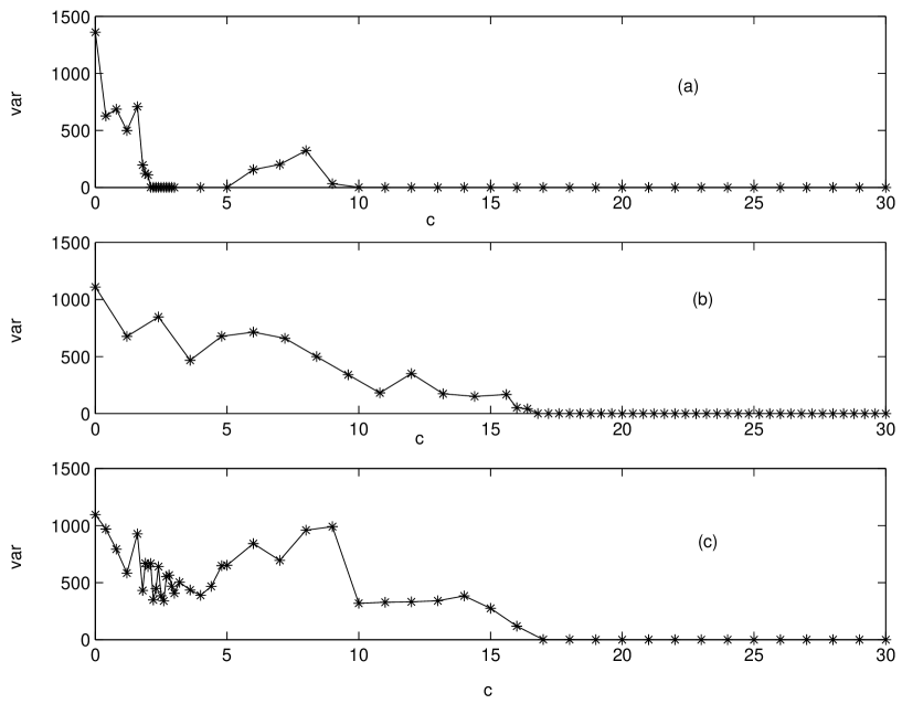
Figure 2: $var$ with respect to $c$ : (a) for the graph 1; (b) for the graph 2; (c) for the graph 3, respectively.

where $\bar{x}_{k}=\frac{1}{\#\mathcal{C}_{k}}\sum_{i\in\mathcal{C}_{k}}x^{i}$, $\langle\cdot\rangle$ denotes the time average. The ordinary differential equations (20) are solved by the Runge-Kutta fourth-order formula with a step length 0.01. The time average interval is $[50,100]$ interval . Fig. 2 indicates that for either graph 1, graph 2, or graph 3, the coupled system (20) clustering synchronizes respectively, if the coupling strength is larger than certain threshold value. Instead, for the graph 1, despite the coupled system can synchronize if $c$ is greater than some value (around 10), it can also synchronize if $c\in[2.2,5]$). It is not very surprising. Previous theoretical results only give sufficient condition that the coupled system can clustering synchronize if the coupling strength $c$ is large enough. It does not exclude the case that the coupled system can still clustering synchronize even if the coupling strength $c$ is small.

The following quantity is used to measure the deviation between clusters:

$${\rm dis}(t)=\min_{i\neq j}[\bar{x}_{i}(t)-\bar{x}_{j}(t)]^{\top}[\bar{x}_{i}(t)-\bar{x}_{j}(t)]$$

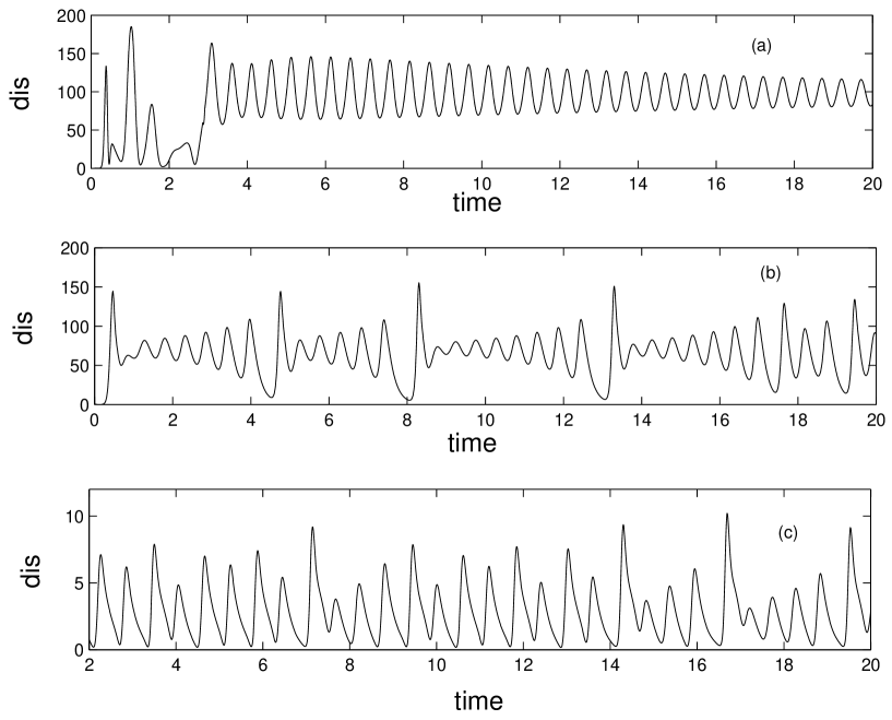
Figure 3: Dynamics of $dis(t)$ through Eq. (12): (a) for the graph 1 with $c=12$; (b) for the graph 2 with $c=25$; (c) for the graph 3 with $c=20$, respectively.

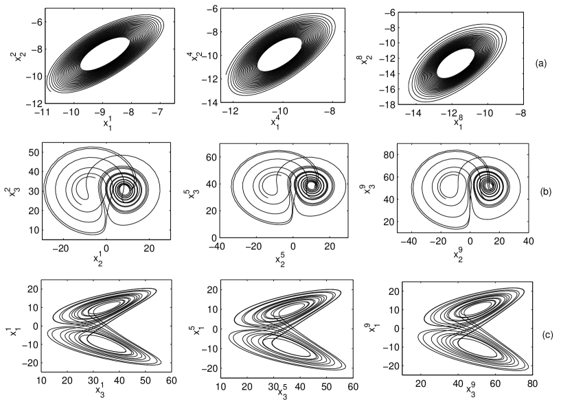
Figure 4: Phase dynamics for each cluster through equality (12): (a) $x_{1}-x_{2}$ phase dynamics for each cluster in the graph 1; (b) $x_{2}-x_{3}$ phase dynamics for each cluster in the graph 2; (2) $x_{3}-x_{1}$ phase dynamics for each cluster in the graph 3, respectively.

Fig.3 shows that the deviation between clusters is apparent, even ”${\rm var}\simeq 0$”. In Fig.4, the dynamical behaviors for all clusters in certain phase plane are given. Although the attractor for each cluster seems to have similar structure and shape, the positions at same time are still different. It is clear that the difference is caused by the different choice of parameters for different clusters. This illustrates that the cluster synchronization is actually realized.

III Adaptive feedback cluster synchronization algorithm

For certain network topology which has weak cluster synchronizability, i.e., the threshold to ensure clustering synchronization is relatively large, which is further studied in Sec. IV.A. It is natural to raise the following question: How to achieve cluster synchronization for networks no matter whether they have ”good” topology or not. One approach proposed recently is adding weights to vertices and edges. Refs Weight showed evidences that certain weighting procedures can actually enhance complete synchronization. On the other hand, adaptive algorithm has emerged as an efficient means of weighting to actually enhance complete synchronizability Adaptive .

In this section, we consider the coupled system

$$\dot{x}^{i}=f_{k}(x^{i})+\sum_{j=1}^{m}a_{ij}w_{ij}\Gamma(x^{j}-x^{i}),~{}i\in\mathcal{C}_{k},~{}k=1,\cdots,K.$$ (25)

and propose an adaptive feedback algorithm to achieve cluster synchronization for a prescribed graph.

Suppose that the common inter-cluster and communicability conditions are satisfied. Without loss of generality, we suppose that the graph $G$ is undirected and connected. Consider the coupled system (2) with Laplacian $L$ defined as in Eqs.(13) and $d^{\top}=[d_{1},\cdots,d_{m}]$ is the left eigenvector of $L$ associated with the eigenvalue $0$.

Now, we propose the following adaptive cluster synchronization algorithm

$$\left\{\begin{array}[]{ll}\dot{x}^{i}(t)=f_{k}(x^{i}(t))+\sum_{j=1}^{m}a_{ij}w_{ij}(t)\Gamma[x^{j}(t)-x^{i}(t)],~{}i\in\mathcal{C}_{k},~{}k=1,\cdots,K,\\ \dot{w}_{ij}(t)=\rho_{ij}d_{i}[x^{i}(t)-\bar{x}^{k}_{d}(t)]^{\top}\Gamma[x^{i}(t)-x^{j}(t)],\\ ~{}{\rm for~{}each}~{}e_{ij}\in\mathcal{E}~{}{\rm and~{}}i\in\mathcal{C}_{k},~{}k=1,\cdots,K\end{array}\right.$$ (29)

with $\rho_{ij}>0$ are constants.

Theorem 3

Suppose that the graph $\mathcal{G}$ is connected, all the assumptions of Theorem 1 hold, the system (29) is essential bounded. The system (29) clustering synchronizes for any initial data.

Proof. First of all, pick $l_{ij}$ as defined in Eqs. (13) and a sufficiently large $c$.Since $\mathcal{G}$ is connected, Theorem 2 tells

$$\bigg{[}D(cL+\alpha I_{m})\bigg{]}^{s}\bigg{|}_{\mathcal{T}_{\mathcal{C}}^{d}(1)}<0.$$ (30)

Define the following candidate Lyapunov function

$$Q_{k}(x,W)=\sum_{i\in\mathcal{C}_{k}}\bigg{[}\frac{d_{i}}{2}(x^{i}-\bar{x}^{k}_{d})^{\top}(x^{i}-\bar{x}^{k}_{d})+\frac{1}{2\rho_{ij}}a_{ij}(w_{ij}-cl_{ij})^{2}\bigg{]},~{}Q(x,W)=\sum_{k=1}^{K}Q_{k}.$$

Differentiating $Q_{k}$, we have

$$\dot{Q}_{k} = \sum_{i\in\mathcal{C}_{k}}d_{i}(x^{i}-\bar{x}^{k}_{d})^{\top}\bigg{\{}f_{k}(x^{i})+\sum_{j=1}^{m}a_{ij}w_{ij}\Gamma(x^{j}-\bar{x}^{j})\bigg{\}}$$

$$+\sum_{i\in\mathcal{C}_{k}}\sum_{k^{\prime}=1}^{K}\sum_{j\in\mathcal{N}_{k^{\prime}}(i)}a_{ij}(w_{ij}-cl_{ij})d_{i}(x^{i}-\bar{x}_{d}^{k})^{\top}\Gamma(x^{i}-x^{j})$$

$$= \sum_{i\in\mathcal{C}_{k}}d_{i}(x^{i}-\bar{x}^{k}_{d})^{\top}\bigg{\{}f_{k}(x^{i})+c\sum_{j=1}^{m}l_{ij}\Gamma(x^{j}-x^{i})-\dot{\bar{x}}_{d}^{k}\bigg{\}}.$$

Similar to the proof of Theorem 1, we have

$$\sum_{i\in\mathcal{C}_{i}}\dot{Q}_{i}=\sum_{i\in\mathcal{C}_{i}}d_{i}(x^{i}-\bar{x}^{k}_{d})^{\top}\bigg{\{}f_{k}(x^{i})-f(\bar{x}_{d}^{k})+c\sum_{j=1}^{m}l_{ij}\Gamma(x^{j}-\bar{x}_{d}^{j})\bigg{\}}$$

and

$$\dot{Q} = \sum_{k=1}^{K}\dot{Q}_{k}\leq-\delta\sum_{k=1}^{K}\sum_{i\in\mathcal{C}_{k}}d_{i}(x^{i}-\bar{x}^{k}_{d})^{\top}(x_{i}-\bar{x}^{k}_{d})$$

$$+\sum_{k=1}^{K}\sum_{i\in\mathcal{C}_{k}}d_{i}(x^{i}-\bar{x}^{k}_{d})^{\top}\bigg{[}\alpha\Gamma(x^{i}-\bar{x}^{k}_{d})+c\sum_{j=1}^{m}l_{ij}\Gamma(x^{j}-\bar{x}_{d}^{j})\bigg{]}$$

$$= -\delta(x-\bar{x}_{d})^{\top}\big{(}D\otimes I\big{)}(x-\bar{x}_{d})+(x-\bar{x}_{d})^{\top}\bigg{\{}[D(cL+\alpha I_{m})]^{s}\otimes\Gamma\bigg{\}}(x-\bar{x}_{d}).$$

Ineq 30 implies

$$\dot{Q}\leq-\delta(x-\bar{x}_{d})^{\top}\big{(}D\otimes I\big{)}(x-\bar{x}_{d})\leq 0.$$

This implies

$$\int_{0}^{t}\delta(x(s)-\bar{x}_{d}(s))^{\top}\big{(}D\otimes I\big{)}(x(s)-\bar{x}_{d}(s))ds\leq Q(0)-Q(t)\leq Q(0)<\infty$$ (31)

From the assumption of the boundedness of Eq.(29), we can conclude $\lim_{t\to\infty}[x(t)-\bar{x}_{d}(t)]=0$ due to the fact that $x(t)$ is uniform continuous. This completes the proof. $\square$

For the disconnected situation, we can split the graph into several connected components and deal with each connected component by the same means as above.

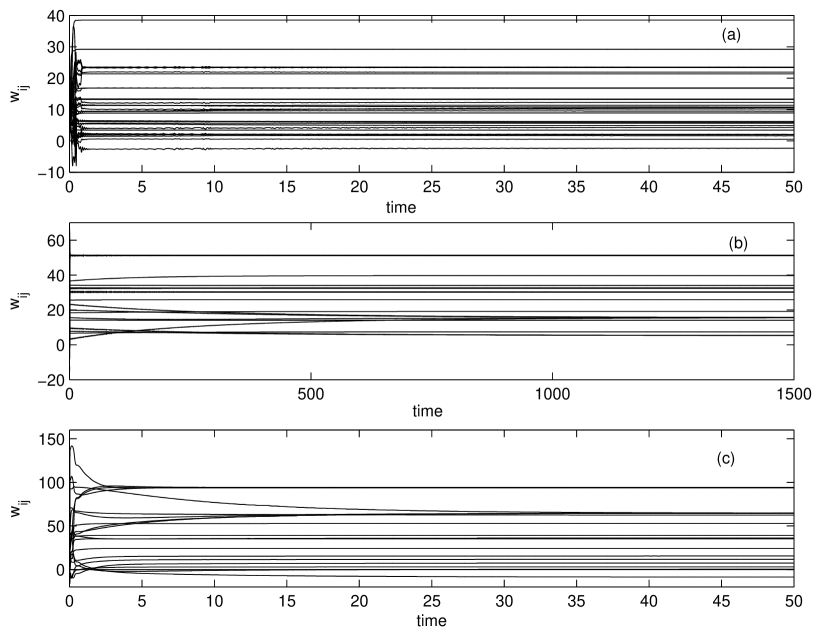
Figure 7: Convergence dynamics of weights $\{w_{ij},~{}(i,j)\in\mathcal{E}\}$ of edges through equality (12) with the adaptive algorithm (29): (a) for the graph 1; (b) for the graph 2; (c) for the graph 3, respectively.

The dynamics of the weights $w_{ij}(t)$ is an interesting issue. Even though it is illustrated in Fig. 7 that all weights converge, to our best reasoning, we can only prove that all intra-weights converge, i.e., vertices $i$ and $j$ belonging to the same cluster $\mathcal{C}_{k}$. In fact, by (31), we have

$$\int_{0}^{\infty}[x^{i}(\tau)-\bar{x}^{k}_{d}(\tau)]^{\top}[x^{i}(\tau)-\bar{x}^{k}_{d}(\tau)]d\tau<+\infty.$$

Thus,

$$\int_{0}^{\infty}|\dot{w}_{ij}(\tau)|d\tau=\rho_{ij}d_{i}\int_{0}^{\infty}\bigg{|}[x^{i}(\tau)-\bar{x}^{k}_{d}(\tau)]^{\top}\Gamma[x^{i}(\tau)-x^{j}(\tau)]\bigg{|}d\tau$$

$$\leq \int_{0}^{\infty}\rho_{ij}d_{i}\|\Gamma\|_{2}\bigg{\{}\big{|}[x^{i}(\tau)-\bar{x}^{k}_{d}(\tau)]^{\top}[x^{i}(\tau)-\bar{x}^{k}_{d}(\tau)]\big{|}+\big{|}[x^{i}(\tau)-\bar{x}^{k}_{d}(\tau)]^{\top}[x^{j}(\tau)-\bar{x}^{k}_{d}(\tau)]\big{|}\bigg{\}}d\tau$$

$$\leq \rho_{ij}d_{i}\|\Gamma\|_{2}\bigg{\{}\frac{3}{2}\int_{0}^{\infty}[x^{i}(\tau)-\bar{x}^{k}_{d}(\tau)]^{\top}[x^{i}(\tau)-\bar{x}^{k}_{d}(\tau)]d\tau$$

$$+\frac{1}{2}\int_{0}^{\infty}[x^{j}(\tau)-\bar{x}^{k}_{d}(\tau)]^{\top}[x^{j}(\tau)-\bar{x}^{k}_{d}(\tau)]d\tau\bigg{\}}.$$

Therefore, for any $\epsilon>0$, there exists $T>0$, such that for any $t_{1}>T$, $t_{2}>T$, we have

$$|w_{ij}(t_{2})-w_{ij}(t_{1})|\leq\int_{t_{1}}^{t_{2}}|\dot{w}_{ij}(\tau)|d\tau<\epsilon$$

By Cauchy convergence principle, $w_{ij}(t)$ converges to some final weights $w_{ij}^{*}$ for $i\in\mathcal{C}_{k}$, $j\in\mathcal{C}_{k}$ when $t\rightarrow\infty$.

On the other hand, to our best reasoning, we can not prove whether or not the weights $w_{ij}(t)$ converges, if the vertex $i$ and $j$ belong to different clusters. If we assume the convergence of all weights, according to the the LaSalle invariant principle, the final weights should guarantee that the cluster synchronization manifold is still invariant. That is to say, if difference trajectories: $s^{k^{\prime}}-s^{k}$ in Eqs. (5), are linearly independent, the cluster the condition (6) still holds for the final weights.

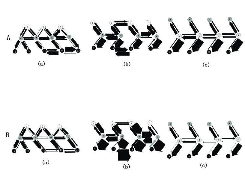
Figure 8: Two sets of the final weighted topologies of the three graphs in Fig. 1 via employing the adaptive algorithm (29) with two different sets of initial data but the same parameters. Set A and B correspond two set of initial values and (a)-(c) correspond the graph 1-3 in Fig. 1. The color of the line represents the sign of the weights (black for positive and gray for negative) and the width of the line represents the scale of the weight in modulus.

Moreover, we have found out that the final weights in our example sensitively depends on the initial values. Fig. 8 gives two sets of weighted topologies of the three graphs as shown in Fig. 1 after employing the adaptive algorithm with two different sets of initial values of $w_{ij}(0)$ and the same parameters. One can see that the final weight can be quite different for different initial values and even be negative. From this observation, we argue that it may be the adaptive process not the final weights counts to reach cluster synchronization. The further investigation of the final weights is out of the scope of the current paper.

III.1 Examples

We still use the graphs 1-3 described in Fig.1 and the Lorenz system (24) as the uncoupled system to illustrate the adaptive feedback algorithms. The ordinary differential equations are solved by the the Runge-Kutta fourth-order formula with a step length 0.01. The initial values of the states and the weights are randomly picked in $[-3,3]$ and $[-5,5]$ respectively. We use the following quantity to measure the state variance inside each cluster with respect to time.

$$K(t)=\sum_{k=1}^{K}\frac{1}{\#\mathcal{C}_{k}-1}\sum_{i\in\mathcal{C}_{k}}[x^{i}(t)-\bar{x}_{k}(t)]^{\top}[x^{i}(t)-\bar{x}_{k}(t)]$$

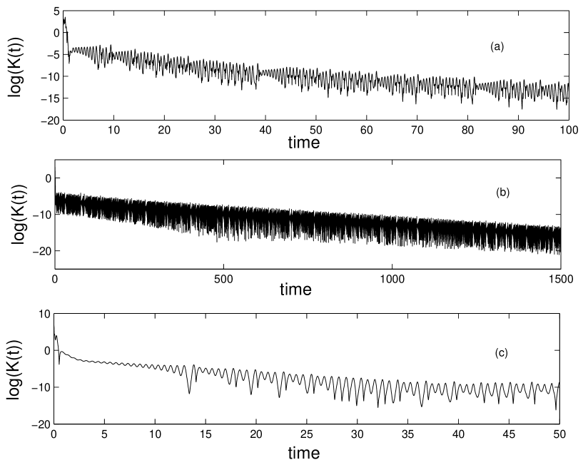
Figure 5: Dynamics of the logarithm of $K(t)$ through equality (12) with the adaptive algorithm (29): (a) for the graph 1; (b) for the graph 2; (c) for the graph 3, respectively.

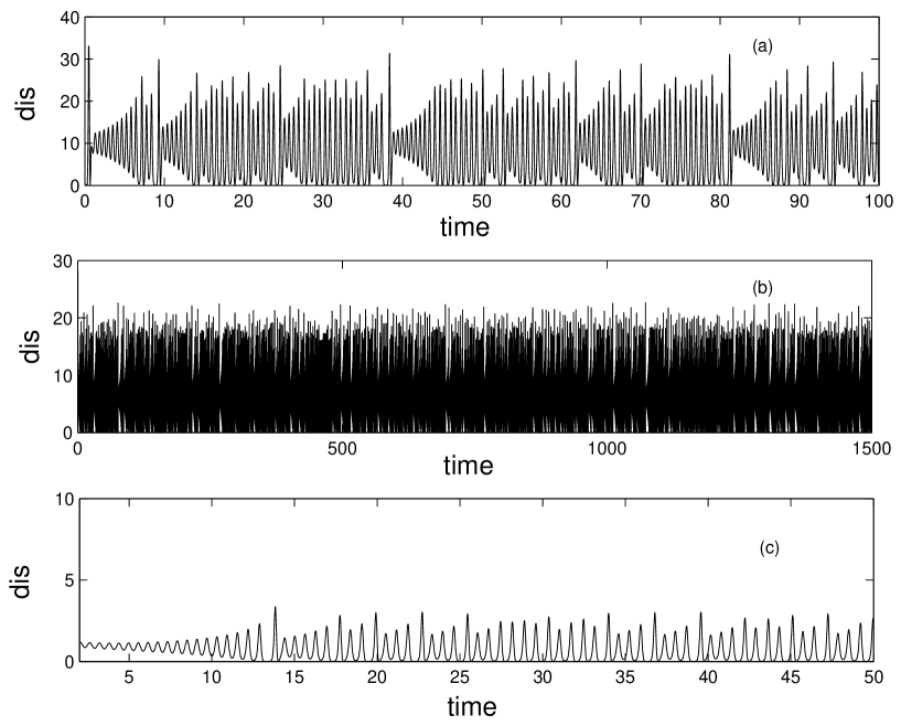
Figure 6: Dynamics of $dis(t)$ through equality (12) with the adaptive algorithm (29): (a) for the graph 1; (b) for the graph 2; (c) for the graph 3, respectively.

Fig.5 shows that the adaptive algorithm succeeds in clustering synchronizing the network with respect to the pre-given clusters. Figs.6 indicates that the differences between clusters due to non-identical parameters $b_{k}$. As shown in Fig.7, the weights converge but the limit values are not always positive. This is not surprising. The right-hand side of the algorithm (29) can be either positive or negative, which causes some weights of edges to be negative. The situation of negative weights is out of the scope of this paper.

IV Discussions

In this section, we make further discussions for some interesting relating issues.

IV.1 Clustering synchronizability

Synchronizability is used to measure the capability of of synchronization for the graph. It can be described by the threshold of the coupling strength to guarantee that the coupled system can synchronize. For complete synchronization, it was formulated as a function of the eigenvalues of symmetric Laplacian Loc_syn or certain Rayleigh quotient of asymmetric Laplacian Wu2 . How the topology of the underlying graph affects synchronizability is an important issue for the study of complex networks Boc1 . Here, similarly, we are also interested in how to formulate and analyze the cluster-synchronizability of a graph $\mathcal{G}$ and a clustering $\mathcal{C}$.

Consider the model (13) of coupled system. Theorem 1 tells us that under the common inter-cluster condition, the cluster synchronization condition (14) can be rewritten as

$$c>\frac{\alpha}{\min_{u\in\mathcal{T}_{\mathcal{C}}^{d}(1),~{}u\neq 0}\frac{-u^{\top}(DL)^{s}u}{u^{\top}Du}}$$ (32)

for some positive definite diagonal $D$. Therefore, we take the Rayleigh-Hitz quotient

$$CS_{\mathcal{G},\mathcal{C}}=\max_{D\in\mathcal{D}}\min_{u\in\mathcal{T}_{\mathcal{C}}^{d}(1),~{}u\neq 0}\frac{-u^{\top}(DL)^{s}u}{u^{\top}Du},$$

to measure the cluster synchronizability for the graph $\mathcal{G}$ and clustering $\mathcal{C}$, where $\mathcal{D}$ denotes the set of positive definite diagonal matrices of dimension $m$. It can be seen that the larger $CS_{\mathcal{G},\mathcal{C}}$ is, the smaller the coupling strength $c$ can be such that the coupled system (13) clusteringly synchronize. In particular, if $L$ is symmetric, then $CS_{\mathcal{G},\mathcal{C}}$ is just the maximum eigenvalue of $-L$ in the transverse space $\mathcal{T}_{C}^{e}(1)$, where $e=[1,1,\cdots,1]^{\top}$. It is an interesting topic that how the two schemes (self-organization and driving) affect the cluster synchronizability for a given graph topology and will be a topic in the future.

Re-consider the examples in Sec.II.D, we can use Matlab LMI and Control Toolbox to obtain the numerical values of $CS_{\mathcal{G},\mathcal{C}}$ for three graphs shown in Fig. 1. Thus, we can derive their values: $0.472$, $0.178$, and $0.172$, respectively. Notwithstanding the right-hand of the Lorenz system does not satisfy the decreasing condition globally, as detailed analyzed in Ref. XC , the trajectory of the coupled Lorenz systems is essentially bounded, of which the bound is independent of the coupling strength $c$. So, concentrating on the bounded terminal region of all trajectories, the decreasing condition can be satisfied and $\alpha$ can be estimated . Here, we get $\alpha\approx 119.3021$, $120.9882$, and $114.6048$, respectively. Thus, we obtain estimations of the infimum of $c$: $252.795$ for the graph 1, $766.892$ for the graph 2, and $667.9655$ for the graph 3. The details of reasoning and algebras are omitted here. It is clear that they all locate in the region of cluster synchronization as numerically illustrated in fig. 2 but less accurate since the estimations are rather loose.

IV.2 Generalized weighted topologies

Previous discussions can also be available toward the coupled system (2) with general weights.

$$\dot{x}^{i}=f_{k}(x^{i})+\sum_{j=1}^{m}a_{ij}w_{ij}\Gamma(x^{j}-x^{i}),~{}i\in\mathcal{C}_{k},~{}k=1,\cdots,K.$$ (33)

Here, the graph may be directed, i.e., $a_{ij}=1$, if there is an edge from vertex $j$ to vertex $i$, otherwise, $a_{ij}=0$. Weights are even not required positive. For the existence of invariant cluster synchronization manifold, we assume

$$\sum_{j\in\mathcal{N}_{k^{\prime}}(i)}w_{ij}=\sum_{j^{\prime}\in\mathcal{N}_{k^{\prime}}(i^{\prime})}w_{i^{\prime}j^{\prime}}$$ (34)

holds for all $i,i^{\prime}\in\mathcal{C}_{k}$ and $k\neq k^{\prime}$. Define its Laplacian $G=[g_{ij}]_{i,j=1}^{m}$ as follows.

$$g_{ij}=\left\{\begin{array}[]{ll}w_{ij}&a_{ij}=1\\ 0&i\neq j{\rm~{}and~{}}a_{ij}=0\\ -\sum\limits_{k=1,k\neq i}^{m}g_{ik}&i=j\end{array}\right..$$

Thus, Eq. (33) becomes

$$\dot{x}^{i}=f_{k}(x^{i})+\sum_{j=1}^{m}g_{ij}\Gamma x^{j},~{}i\in\mathcal{C}_{k},~{}k=1,\cdots,K.$$ (36)

Replacing $cl_{ij}$ by $g_{ij}$ and following the routine of the proof of theorem 1, we can obtain following result.

Theorem 4

Suppose that the common inter-cluster coupling condition (34) is satisfied, each $f_{k}(\cdot)-\alpha\Gamma\cdot$ satisfies the decreasing condition for some $\alpha\in\mathbb{R}$, and $\Gamma$ is nonnegative definite. If there exists a positive definite diagonal matrix $D$ such that

$$\bigg{[}D(G+\alpha I_{m})\bigg{]}^{s}_{\mathcal{T}_{\mathcal{C}}^{d}(1)}\leq 0$$ (37)

holds, then the coupled system (36) can clustering synchronize with respect to the clustering $\mathcal{C}$.

And, we use the same discussions as in theorem 2 to obtain the following general result.

Theorem 5

Suppose that the common inter-cluster coupling condition (7) is satisfied. For a bi-directed unweighted graph $\mathcal{G}$, there exist positive weights to the graph $\mathcal{G}$ such that Ineq. (37) holds if and only if all vertices in the same cluster belongs to the same connected component in the graph $\mathcal{G}$.

In fact, the proofs of theorems 4 and 5 simply repeats those of theorems 1 and 2, respectively.

Ref. Sor is a paper closely relating to this paper. Here, we give some comparisons. First, investigated the local cluster synchronization of inter-connected clusters by extending the master stability function method. Instead, in this paper, we are concerned with the global cluster synchronization. Second, the models discussed are different. The topologies discussed in Sor exclude intra-cluster couplings. In this paper, we consider more general graph topology. Third, Ref. Sor studied the situation of nonlinear coupling function and we consider the linear case. Despite that Ref. Sor considered different coupling stengths for clusters and we consider a common one in Sec. II, theorem 4 can apply to discussion of such models proposed in Ref. Sor .

V Conclusions

The idea for studying synchronization in networks of coupled dynamical systems sheds light on cluster synchronization analysis. In this paper, we study cluster synchronization in networks of coupled non-identical dynamical systems. Cluster synchronization manifold is defined as that the dynamics of the vertices in the same cluster are identical. The criterion for cluster synchronization is derived via linear matrix inequality. The differences between clustered dynamics are guaranteed by the non-identical dynamical behaviors of different clusters. The algebraic graph theory tells that the communicability between each pair of vertices in the same cluster is a doorsill for chaos cluster synchronization. This leads an description of two schemes to realize cluster synchronization: self-organization and driving. One can see that the latter scheme implies that cluster synchronization can be realized in a non-clustered networks, for example, the graph 2 in the Fig. 1. Adaptive feedback algorithm is used to enhance cluster synchronization motions.

Appendix

In this appendix, for each positive $d$, we give the details to find a $u\in\mathcal{T}_{\mathcal{C}}^{d}(1)$ with $u\neq 0$ such that $u^{\top}DLu=0$ in the case that there exists a cluster $\mathcal{C}_{1}$ that does not belong the same connected component. Without loss of generality, suppose $L$ has form:

$$L=\left[\begin{array}[]{ll}L_{1}&0\\ 0&L_{2}\end{array}\right].$$

Let $\mathcal{V}_{1}$ and $\mathcal{V}_{2}$ corresponds the sub-matrices $L_{1}$ and $L_{2}$ respectively. And, $\mathcal{C}_{1}\bigcap\mathcal{V}_{i}\neq\emptyset$ for all $i=1,2$. We consider two situations. First, in the case that $\mathcal{C}_{1}$ is isolated from other clusters. In other words, there are no edges between $\mathcal{C}_{1}$ and other clusters. Let

$$u_{i}=\left\{\begin{array}[]{ll}\alpha&i\in\mathcal{C}_{1}\bigcap\mathcal{V}_{1}\\ \beta&i\in\mathcal{C}_{1}\bigcap\mathcal{V}_{2}\\ 0&{\rm otherwise}\end{array}\right..$$

Let $a=\sum_{j\in\mathcal{C}_{1}\bigcap\mathcal{V}_{1}}d_{j}$ and $b=\sum_{j\in\mathcal{C}_{1}\bigcap V_{2}}d_{j}$. Then, if picking $\alpha$ and $\beta$ satisfying $a\alpha+b\beta=0$ with $\alpha,\beta\neq 0$, then $u\in\mathcal{T}_{\mathcal{C}}^{d}(1)$ holds. In addition, $u^{\top}DLu=0$ due to $Lu=0$.

In the case that $\mathcal{C}_{1}$ is not isolated, suppose there are totally $K$ clusters, and $L_{1}$ and $L_{2}$ are both connected (otherwise, we only consider the connection parts of $L_{1}$ and $L_{2}$ that contain vertices from $\mathcal{C}_{1}$), due to the common inter-cluster coupling condition, and the absence of isolated cluster, we have $\mathcal{C}_{i}\bigcap\mathcal{V}_{j}\not=\emptyset$ holds for all $i=1,\cdots,K$ and $j=1,2$. Pick a vector $u=[u_{1},\cdots,u_{m}]^{\top}$ with

$$u_{i}=\left\{\begin{array}[]{ll}\alpha_{k}&i\in\mathcal{C}_{k}\bigcap\mathcal{V}_{1}\\ \beta_{k}&i\in\mathcal{C}_{k}\bigcap\mathcal{V}_{2},\end{array}\right.$$

Denote $d_{k}^{1}=\sum_{i\in\mathcal{C}_{k}\bigcap\mathcal{V}_{1}}d_{i}$, $d_{k}^{2}=\sum_{i\in\mathcal{C}_{k}\bigcap\mathcal{V}_{2}}d_{i}$, and $\bar{u}_{1}=[\alpha_{1},\cdots,\alpha_{K}]^{\top}$, $\bar{u}_{2}=[\beta_{1},\cdots,\beta_{K}]^{\top}$, $\bar{u}=[\bar{u}_{1}^{\top},\bar{u}_{2}^{\top}]^{\top}$, $\bar{D}_{1}={\rm diag}[d_{1}^{1},\cdots,d_{K}^{1}]$, $\bar{D}_{2}={\rm diag}[d_{1}^{2},\cdots,d_{K}^{2}]$, and $\bar{D}={\rm diag}[\bar{D}_{1},\bar{D}_{2}]$. Define a $K\times K$ matrix $W^{1}$ from $L_{1}$ in such way that for $i\not=j$, $W^{1}_{ij}=1$ if there’s interaction between cluster $i$ and $j$, and $W^{1}_{ij}=0$ otherwise. $W^{1}_{ii}=-\sum\limits_{j=1,j\not=i}^{K}W^{1}_{ij}$. Define $W^{2}$ in the same way according to $L_{2}$, due to the common inter-cluster condition, it is easy to see that $W^{1}=W^{2}$. Denote $W={\rm diag}[W^{1},W^{2}]$.

After computation, we have that for any given positive definite diagonal matrix $D={\rm diag}[d_{1},\cdots,d_{m}]$, $u^{\top}DLu=\bar{u}^{\top}\bar{D}W\bar{u}$ holds. For $u\in\mathcal{T}_{\mathcal{C}}^{d}$, $\bar{u}_{2}=-\bar{D}_{1}\bar{D}_{2}^{-1}\bar{u}_{1}$. Denote $v=\bar{D}_{1}\bar{u}_{1}$, we have $\bar{u}^{\top}\bar{D}W\bar{u}=[v^{\top}v^{\top}]W\bar{D}^{-1}[v^{\top}v^{\top}]^{\top}=v^{\top}W^{1}(\bar{D}_{1}^{-1}+\bar{D}_{2}^{-1})v$. This implies that if we can find $v$ satisfying $v^{\top}W^{1}(\bar{D}_{1}^{-1}+\bar{D}_{2}^{-1})v=0$, then there exists $u\in\mathcal{T}_{\mathcal{C}}^{d}(1)$ such that $u^{\top}DLu=0$. Since $W^{1}(\bar{D}_{1}^{-1}+\bar{D}_{2}^{-1})$ has rank at most $K-1$, we can pick $v$ as the eigenvector corresponding to the zero eigenvalue of $W^{1}(\bar{D}_{1}^{-1}+\bar{D}_{2}^{-1})$, and this completes the proof.

In summary, in both situations, we can find certain nonzero vector $u$ belonging to the transverse space $\mathcal{T}_{\mathcal{C}}^{d}(1)$ and $u^{\top}DLu=0$.

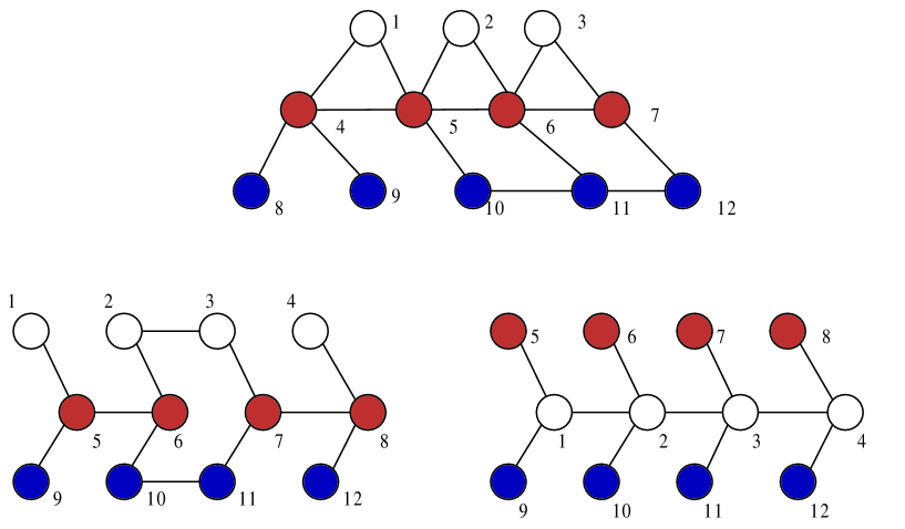
Figure 1: Graphs of examples. In the graph 1, the white cluster (vertex set $1-3$) is driven since they has no intra-cluster edges, the red cluster (vertex set $4-7$) is mixed since each pari of vertices can access each other via only inter- or intra- edges, and the blue cluster is driven since each pair of vertices can access each other via only the inter-cluster edges but can not communicate only via intra-cluster edges. In the graph 2, each cluster of the white and blue clusters (vertex sets $1-4$ and $9-12$) is driven since each pair of vertices can access each other only via inter-cluster edges but only has a single intra-cluster edges. However, the read cluster (vertex set $5-8$) is recognized as a hybrid cluster since the sets of inter- or intra-cluster edges are both necessary for communication between each pair of vertices. In the graph 3, the red and blue clusters (vertex sets $5-8$ and $9-12$) are all driven since they do not have intra-cluster edges and the white cluster (vertex set $1-4$) is an example of self-organization since each pair of vertices can communicate via only the intra-cluster edges but can not if removing the intra-cluster edges.

References

• (1) A. Pikovsky, M. Roseblum, J. Kurths, Synchronization: A universal concept in nonlinear sciences ( Cambridge University Press, 2001).
• (2) S. Boccaletti, V. Latora, Y. Moreno, M. Chavez, D.-U. Hwang, “Complex networks: structure and dynamics”, Phys. Rep., 424, 175 (2006).
• (3) X. F. Wang, G. Chen, “Complex networks: small-world, scale-free and beyond”, IEEE Circ. Syst. Mag., 3:1, 6 (2003).
• (4) H. Fujisaka, T. Yamada, Prog. Theor. Phys., 69, 32 (1983); 72, 885 (1984); V. S. Afraimovich, N. N. Verichev, M. I. Rabinovich, Izv. Vyssh. Uchebn. Zaved. Radiofiz., 29, 795 (1986).
• (5) S. H. Strogatz, I. Stewart, Sci. Amer., 269:6, 102 (1993).
• (6) C. M. Gray, J. Comput. Neurosci., 1:11, 38 (1994).
• (7) L. Glass, Nature, 410, 277 (2001).
• (8) S. Boccaletti, J. Kurths, G. Osipov, D. L. Valladares, C. S. Zhou, Phys. Rep., 366, 1 (2002).
• (9) L. M. Pecora, T. L. Carroll, Phys. Rev. Lett., 64:8, 821 (1990); J. F. Heagy, T. L. Carroll, L. M. Pecora, Phys. Rev. E., 50, 1874 (1994).
• (10) P. Ashwin, J. Buescu, I. Stewart, Nonlinearity, 9 703 (1996).
• (11) J. Jost, M. P. Joy, Phys. Rev. E, 65, 016201 (2001); X. F. Wang, G. Chen, IEEE Trans. Circ. Syst.-1, 49:1, 54 (2002); G. Rangarajan, M. Ding: Phys. Lett. A, 296, 204 (2002); Y. H. Chen, G. Rangarajan, and M. Ding: Phys. Rev. E., 67, 026209 (2003).
• (12) C. W. Wu, L. O. Chua, IEEE Trans. Circ. Syst.-1, 42:8, 430 (1995).
• (13) I. V. Belykh, V. N. Belykh, M. Hasler, Physica D, 195, 159 (2004) and 188 (2004);J. Cao, P. Li, W. Wang, Phys. Lett. A, 353, 318 (2006).
• (14) W. Lu, T. Chen, Physica D, 213, 214 (2006).
• (15) C. W. Wu, Nonlinearity, 18, 1057 (2005).
• (16) A. Schnitzler, J. Gross, Nat. Rev. Neurosci, 6, 285 (2005).
• (17) P. R. Chandler, M. Patcher, S. Rasmussen, Proceedings of the American Control Society, 20 (2001); K. M. Passino, IEEE Control Syst. Mag., 22, 52 (2002); J. Finke, K. Passino, A. G. Sparks, IEEE Control Syst. Mag., 14, 789 (2006).
• (18) B. Blasius, A. Huppert, L. Stone, Nature (London), 399, 354 (1999); E. Montbrió, J. Kurths, B. Blasius, Phy. Rev. E, 70, 056125 (2004).
• (19) N. F. Rulkov, Chaos, 6, 262 (1996).
• (20) L. Stone, R. Olinky, B. Blasius, A. Huppert, B. Cazelles, Proceedings of the Sixth Experimental Chaos Conference, AIP Conf. Proc. No. 662, 476 (2002).
• (21) E. Jones, B. Browning, M. B. Dias, B. Argall, M. Veloso, A. Stentz, Proceedings IEEE International Conference on Robotics and Automation, Orlando, 2006, 570-575; K. -S, Hwang, S. -W. Tan, C. -C. Chen, IEEE Trans. Fuzzy Syst., 12, 569 (2004).
• (22) V. N. Belykh, I. V. Belykh, M. Hasler, Phy. Rev. E, 62, 6332 (2000); V. N. Belykh, I. V. Belykh, E. Mosekilde, Phys. Rev. E, 63 036216 (2001).
• (23) Z. Ma, Z. Liu, G. Zhang, Chaos, 16, 023103 (2006).
• (24) W. Wu, T. Chen, Physica D, 238, 355 (2009); W. Wu, W. Zhou, T. Chen, IEEE T. Circuits Syst.-I, in press, (2008);
• (25) S. Jalan, R. E. Amritkar, Pys. Rev. Lett., 90:1, 014101 (2003); S. Jalan, R. E. Amritkar, C.-K. Hu, Phys. Rev. E, 72, 016211 (2005); 016212 (2005).
• (26) F. Sorrentino, E. Ott, Phys. Rev. E, 76, 056114 (2007).
• (27) L. Chen, J. Lu, J. Syst. Sci. Complexity, 20, 21 (2008).
• (28) I. V. Belykh, V. N. Belykh, M. Hasler, Chaos, 13:1, 165 (2003).
• (29) Q.-C. Pham, J.-J. Slotine, Neural Networks, 20, 62 (2007).
• (30) W. Lohmiller, J.-J. Slotine, Automatica, 34:6, 671 (1998).
• (31) “Special issue on nonlinear waves, patterns, and spatiotemporal chaos in dynamical arrays”, edited by L. O. Chua, IEEE Trans. Circ. Syst., 42 (1995).
• (32) P. A. Horn, C. R. Johnson, Matrix Analysis (Cambridge University Press, New York, 1985).
• (33) J. P. Lasalle, IRE Trans. Circuit Theory 7, 520 (1960).
• (34) M. Chavez, D.-U. Hwang, H. G. E. Hentschel, S. Boocaletti, Phys. Rev. Lett., 94, 218701 (2005); C. Zhou, J. Kurths, Phys. Rev. Lett., 96, 164102 (2006); S. Boccaletti, D.-U. Hwang, M. Chavez, A. Amann, J. Kurths, L. M. Pecora, Phys. Rev. E, 74, 016102 (2006); C. S. Zhou, A. E. Motter, J. Kurths, Phys. Rev. Lett., 96, 034101 (2006).
• (35) X. Liu, T. Chen, Physica D, 237, 630 (2008).
• (36) J. Lu, J. Cao, Chaos, 15, 043901 (2005); D. Huang, Phys. Rev. E, 71, 037203 (2005); J. Zhou, J-A. Lu, J. Lü, IEEE Trans. Automatic Control, 51:4, 652 (2006); W. Lu, Chaos, 17, 023122 (2007).
• (37) The reason why we choose initial time for average from 50 not 0 is that even if the coupled system synchronizes clustering, the variance as calculated by ${\rm var}$ can be very large ($>10^{3}$). This implies that it will take a very long time for average to make the variance is near zero. To save calculationg amount, we pick the inital time apart from zero.
• (38) Our theoretical result (proposition 1) can only intepret the case the coupled system can clustering synchronize if the coupling strength $c$ is large enough. As shown by Fig. 2, the coupled system (12) over the graphs 2 and 3 can clustering synchronize only if the coupling strength $c$ is greater than some threshold. But, for the graph 1, despite the coupled system can synchronize if $c$ is greater than some value (around 10), there exists an interval (about $[2.2,5]$) of $c$ by which the system synchronizes. This can not be interpreted via our theoretical result.
Refer to caption