Iterated maps for clarinet-like systems

Abstract

The dynamical equations of clarinet-like systems are known to be reducible to a non-linear iterated map within reasonable approximations. This leads to time oscillations that are represented by square signals, analogous to the Raman regime for string instruments. In this article, we study in more detail the properties of the corresponding non-linear iterations, with emphasis on the geometrical constructions that can be used to classify the various solutions (for instance with or without reed beating) as well as on the periodicity windows that occur within the chaotic region. In particular, we find a regime where period tripling occurs and examine the conditions for intermittency. We also show that, while the direct observation of the iteration function does not reveal much on the oscillation regime of the instrument, the graph of the high order iterates directly gives visible information on the oscillation regime (characterization of the number of period doubligs, chaotic behaviour, etc.).

Keywords : Bifurcations, Iterated maps, Reed musical instruments, Clarinet, Acoustics.

1 Introduction

Non-linear iterated maps are now known as an universal tool in numerous scientific domains, including for instance mechanics, hydrodynamics and economy [1] [2] [3]. They often appear because the differential equations describing the dynamics of a system can be reduced to non-linear iterations, with the help of Poincaré recurrence maps for instance. The resulting iterations combine a great mathematical simplicity, which makes them convenient for numerical simulations, with a large variety of interesting behaviors, providing generic information on the properties of the system. In particular, they are essential to characterize one of the routes to chaos, the cascade of period doublings [4].

In musical acoustics, Mc Intyre et al. have given, in a celebrated article [5], a general frame for calculating the oscillations of musical instruments, based upon the coupling of a linear resonator and a non-linear excitator (for reed instruments, the flow generated by a supply pressure in the mouth and modulated by a reed). In an appendix of their article they show that, within simplified models of self-sustained instruments, the equations of evolution can also be reduced to an iterated map with appropriate non-linear functions. For resonators with a simple shape such as a uniform string or a cylindrical tube, the basic idea is to choose variables that are amplitudes of the incoming and outgoing waves (travelling waves), instead of usual acoustic pressure and volume velocity in the case of reed instruments. If the inertia of the reed is ignored (a good approximation in many cases), and if the losses in the resonator are independent of frequency, the model leads to simple iterations; the normal oscillations correspond to the so called “Helmholtz motion”, a regime in which the various physical quantities vary in time by steps, as in square signals. Square signals obviously are a poor approximation of actual musical signals, but this approach is sufficient when the main purpose is to study regimes of oscillation, not tone-color.

In the case of clarinet-like systems, the idea was then expanded [6], giving rise to experimental observations of period doubling scenarios and to considerations on the relations between stability of the regimes and the properties of the second iterate of the non-linear function; see also [7] and especially [8] for a review of the properties of iterations in clarinet-like systems and a discussion of the various regimes (see also [9]). More recent work includes the study of oscillation regimes obtained in experiments [10, 11], computer simulation [12] as well as theory [13, 14].

The general form of the iteration function that is relevant for reed musical instruments is presented in section 3. It it is significantly different from the usual iteration parabola (i.e. the so-called logistic map). Moreover, it will be discussed in more detail that the control parameters act in a rather specific way, translating the curve along an axis at $45^{\circ}$ rather than acting as an adjustable gain.

The purpose of the present article is to study the iterative properties of functions having this type of behavior, and their effect on the oscillation regimes of reed musical instruments. We will study the specificities and the role of the higher order iterates of this class of functions, in particular in the regions of the so called “periodicity windows”, which take place beyond the threshold of chaos. These windows are known to contain interesting phenomena [2, 15, 16], for instance period tripling or a route to intermittence, which to our knowledge have not yet been studied in the context of reed musical instruments. Moreover, the iterates give a direct representation of the zones of stability of the different regimes (period doublings for instance), directly visible on the slope of the corresponding iterate.

For numerical calculations, it is necessary to select a particular representation of the non-linear function, which in turn requires to choose a mathematical expression of the function giving the volume flow rate as a function of the pressure difference across the reed. A simple and realistic model of the quasi-static flow rate entering a clarinet mouthpiece was proposed in 1974 by Wilson and Beavers [17], and discussed in more detail in 1990 by Hirschberg et al. [18]. This model provides a good agreement with experiments [19] and leads to realistic predictions concerning the oscillations of a clarinet [20]. Using this mathematical representation of the flow rate, we will see that iterations lead to a variety of interesting phenomena. Our purpose here is not to propose the most elaborate possible model of the clarinet, including all physical effects that may occur in real instruments. It is rather to present general ideas and mathematical solutions as illustration of the various class of phenomena that can take place, within the simplest possible formalism; in a second step, one can always take this simple model as a starting point, to which perturbative corrections are subsequently added in order to include more specific details.

We first introduce the model in § 2, and then discuss the properties of the iteration function in § 3. The bifurcations curves are obtained in § 4 and, in § 5, we discuss the iterated functions and their applications in terms of period tripling and intermittence. In particular we see how the graph of high order iterates give visible information on the regime of oscillation (number of period doublings for instance) or the appearance of a chaotic regime, while nothing special appears directly in the graph of the first iterate. Two appendices are added at the end.

2 The model

We briefly recall the basic elements of the model, the non-linear characteristics of the excitator, and the origin of the iterations within a simplified treatment of the resonator.

2.1 Nonlinear characteristics of the entering flow

In a quasi static regime, the flow $U$ entering the resonant cavity is modelled with the help of an approximation of the Bernoulli equation, as discussed e.g. in [18]. We note $P_{int}$ the acoustic pressure inside the mouthpiece, assumed to be equal to the one at the output of the reed channel, $P_{m}$ the pressure inside the mouth of the player; for small values of the difference:

$$\Delta P=P_{m}-P_{int}\text{ ,}$$ (1)

the reed remains close to its equilibrium position, and the conservation of energy implies that $U$ is proportional to $\eta_{p}\sqrt{\left|\Delta P\right|}$, where $\eta_{p}=\pm 1$ is the sign of $\Delta P$ (we ignore dissipative effects at the scale of the flow across the reed channel); for larger values of this difference, the reed moves and, when the difference reaches the closure pressure $P_{c}$, it completely blocks the flow. These two effects are included by assuming that if $\Delta P\leq P_{c}$ the flow $U$ is proportional to $\eta_{p}\sqrt{\left|\Delta P\right|}\left[P_{c}-\Delta P\right]$, and if $\Delta P>P_{c}$, the flow vanishes. Introducing the dimensionless quantities:

$$\begin{array}[]{l}p=P_{int}/P_{c}\\ u=UZ_{\infty}/P_{c}\\ \gamma=P_{m}/P_{c}\text{ }\\ \Delta p=\Delta P/P_{c}=\gamma-p\text{ .}\end{array}$$ (2)

where $Z_{\infty}=\rho c/S$ is the acoustic impedance of an infinitely long cylindrical resonator having the same cross section $S$ than the clarinet bore ($\rho$ is the density of air, $c$ the velocity of sound), we obtain:

$$u = 0$$

$$\text{if \ \ \ }\Delta p>1\text{ \ \ i.e. \ \ \ \ \ \ }p<\gamma-1\text{ \ ;}$$

$$u = \zeta(p+1-\gamma)\sqrt{\gamma-p}$$

$$\text{if }0<\Delta p<1\text{ i.e. \ }\gamma-1<p<\gamma\text{ ;}$$

$$u = -\zeta(p+1-\gamma)\sqrt{p-\gamma}$$

$$\text{if \ \ \ }\Delta p<0\text{ \ i.e. \ \ \ \ \ \ }p>\gamma.$$

The parameter $\zeta$ characterizes the intensity of the flow and is defined as:

$$\zeta=\frac{cS_{op}}{S}\sqrt{\frac{2\rho}{P_{c}}}\text{ ,}$$ (6)

where $S_{op}$ is the opening cross section of the reed channel at rest. One can show that $\zeta$ is inversely proportional to square root of the reed stiffness, contained in $P_{c}$. In real instruments, typical values of the parameters are $\gamma\in\left[0,1.5\right]$; $\zeta=\left[0.1,0.5\right]$ ; values $\zeta>1$ will not be considered here, since they correspond to multi-valued functions $u(p)$, a case that does not seem very realistic in practice. Fig.1 shows an example of function defined in Eqs.(2.1 to 2.1). It is obviously non-analytic; it is made of three separate analytic pieces, with a singular point at $p=\gamma.$ The derivative of the function $u(p)$ is discontinuous at $p=\gamma-1$ (point $M_{b}$ in Fig. 1, the index $b$ being used for the limit of possible beating); a smoothing of the resulting angle of the function could easily be introduced at the price of a moderate mathematical complication, but this is not necessary for the present discussion.

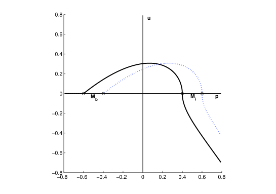
Figure 1: Graph showing the air flow rate $u$ entering the resonator of a clarinet as a function of the internal pressure $p$ (pressure in the mouthpiece). All physical quantities are expressed in dimensionless units, as explained in the text. M_b corresponds to the contact point where the internal pressure in the mouthpiece bends the reed sufficiently to close the channel, so that the flow vanishes; it remains zero in all region $p<\gamma-1$. M_i is the inversion point where $p=\gamma$ and where the acoustic flow changes sign. The full line corresponds to $\gamma=0.4$, the broken line to $\gamma=0.6$. Here $\zeta=0.8$.

2.2 Iteration

Waves are assumed to be planar in the quasi one dimensional cylindrical resonator. Any wave can be expanded into an outgoing wave $p^{+}(t-z/c)$ and an incoming wave $p^{-}(t+z/c)$, where $t$ is the time and $z$ the abscissa coordinate along the axis of the resonator; at point $z=0$ (at the tip of the reed), the acoustic pressure and flow are given by:

$$p(t)=p^{+}(t)+p^{-}(t)\text{ \ \ ; \ \ }u(t)=p^{+}(t)-p^{-}(t)$$ (7)

or:

$$p^{+}(t)=\frac{1}{2}\left[p(t)+u(t)\right]\text{ \ \ ; \ \ }p^{-}(t)=\frac{1}{2}\left[p(t)-u(t)\right].$$ (8)

We will use variables $p^{\pm}(t)$ instead of $p(t)$ and $u(t)$. If we assume that the impedance at the output of the resonator is zero (no external radiation, the output pressure remains the atmospheric pressure), we obtain the reflection condition:

$$p^{-}(t)=-p^{+}(t-2\ell/c)\text{ ,}$$ (9)

where $\ell$ is the resonator length and $c$ the sound velocity. This equation expresses that the reflected wave has the same amplitude than the incoming wave. Losses are not included in this relation, but one can also introduce them very easily by replacing (9) by:

$$p^{-}(t)=-\lambda p^{+}(t-2\ell/c)\text{ ,}$$ (10)

which amounts to introducing frequency independent losses; a typical value is $\lambda=0.9$. For a cylindrical, open, tube with no radiation at the open end so that losses only occur inside the tube, $\lambda=\exp(-2\alpha\ell)$, where $\alpha$ is the absorption coefficient. Of course this is an approximation: real losses are frequency dependent and radiation occurs but, since losses remain a relatively small correction in musical instruments, using Eq. (10) is sufficient for our purposes.

We now assume that all acoustical variables vanish until time $t=0$, and then that the excitation pressure in the mouth suddenly takes a new constant value $\gamma$; this corresponds to a Heaviside step function for the control parameter. Between time $0$ and time $2l/c$, according to (10), the incoming amplitude $p^{-}(t)$ remains zero, but the outgoing amplitude $p^{+}(t)$ has to jump to value $p_{1}^{+}$ in order to fulfil Eqs.(2.1 to 2.1) . At time $t=2l/c$, the variable $p^{-}(t)$ jumps to value $-\lambda p_{1}^{+}$, which immediately makes $p^{+}(t)$ jump to a new value $p_{2}^{+}$, in order to still fulfil Eqs.(2.1 to 2.1). This remains true until time $t=4l/c$, when $p^{-}(t)$ jumps to value $-\lambda p_{2}^{+}$ and $p^{+}(t)$ to a value $p_{3}^{+}$, etc. By recurrence, one obtains a regime where all physical quantities remain constant in time intervals $2nl/c<t<2(n+1)l/c$, in particular $p_{n}$ for the pressure and $u_{n}$ for the flow, with the recurrence relation:

$$p_{n}^{-}=-\lambda p_{n-1}^{+}\text{.}$$ (11)

In what follows, it will be convenient to use $2l/c$ as a natural time unit. We will then simply call “time $n$” the time interval $(n-1)2l/c\leq t<n2l/c$. Notice that in order to get higher regimes (with e.g. triple frequency), the previous choice of transient for $\gamma$ needs to be modified (see e.g.[8]).

Now, by combining Eqs.(2.1 to 2.1) and 7), one can obtain a non-linear relation $g$ between $p_{n}^{+}$ and $p_{n}^{-}$:

$$p_{n}^{+}=g(p_{n}^{-})\text{ ,}$$ (12)

which, combined with (11), provides the relation:

$$p_{n}^{+}=g(-\lambda p_{n-1}^{+})=f(p_{n-1}^{+})\text{,}$$ (13)

with, by definition:   $f(x)\equiv g(-\lambda x).$ The equation of evolution of the system are then equivalent to a simple mapping problem with an iteration function $f(x)$. The graph of this function is obtained by rotating the non-linear characteristics of Fig. 1 by $45^{\circ}$ (in order to obtain $g$), then applying a symmetry (to include the change of sign of the variable) and finally a horizontal rescaling by a factor $1/\lambda$; the result is shown in Fig. 2. This provides a direct and convenient graphical construction of the evolution of the system [6]; Fig. 3 shows how a characteristic point $1$ is transformed into its next iterate $2,$ etc… by the usual construction, at the intersection of a straight line with the iteration curve, i.e. by transferring the value of $f(x)$ to the $x$ axis and reading the value of the function at this abscissa in order to obtain $f\left[f(x)\right]$.

In what follows, we consider $\gamma$ as the main control parameter of the iteration; it corresponds to a change of pressure in the mouth of the instrumentalist. A second control parameter is $\zeta$, which the player can also change in real time by controlling the lip pressure on the reed. For a given note of the instrument, parameter $\lambda$ remains fixed, but of course depends on which lateral holes of the clarinet are closed, in other words on the pitch of the note.

The oscillations where the functions remain constant and jump to a different value at regular interval of times are reminiscent of the Raman regime for the oscillation of bowed strings [22]. Mc Intyre et al. have indeed noticed that, if one replaces the non-linear function by that corresponding to a bowed string, one obtains the Raman oscillation regime of a string bowed at its center [5].

3 Properties of the iteration

The analytical expression of the iteration function is given in Appendix A. Figure 2 shows the function for given values of the parameters $\gamma$ and $\zeta$, and three different values of the loss parameter $\lambda.$

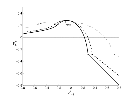
Figure 2: Iteration function $f$ for $\zeta=0.8$ and $\gamma=0.43$  Solid line $\lambda=1$ (no loss in the resonator); mixed line $\lambda=0.8$; dotted line $\lambda=0.4$. The circles on the right indicate the contact point M_b, those on the left the flow inversion point M_i.

In the literature, the most commonly studied functions have the following properties (see e.g. Collet and Eckman [3] or Bergé et al [2]):

• They are defined on a finite interval and map this interval into itself;

• They are continuous;

• They have a unique maximum;

• their Schwarzian derivative is negative.

A function verifying these properties will be called a “standard” function; the function $f(x)$ of interest in our case does not fulfil all these requirements.

Domain of iteration

Usually, the iteration function defines an application of the interval $0\leq x\leq 1$ over itself. Here, $f(x)$ is defined on an infinite interval $\left[-\infty,+\infty\right]$ even if, obviously, very large values of the variables are not physically plausible. Nevertheless, analyzing the different cases corresponding to Eqs.(2.1 to 2.1), one can show that the function $f(x)$ has a maximum $f_{\max}$ obtained for:

$$x_{\max}=-\frac{1}{\lambda}\left[\frac{\gamma}{2}-\frac{5}{18}-\chi\left(\zeta-\frac{5}{3\zeta}\right)\right]$$ (14)

with value:

$$f_{\max}=\frac{\gamma}{2}+A_{\zeta}\text{ with \ }A_{\zeta}=\chi\left(\zeta+\frac{1}{3\zeta}\right)-\frac{1}{18}\text{ }$$ (15)

where $\chi$ is defined by:

$$\chi=\frac{1}{9}\left[\sqrt{3+\frac{1}{\zeta^{2}}}-\frac{1}{\zeta}\right]\text{ .}$$ (16)

It can be shown that this maximum is unique for large value of $\zeta$ ($\zeta>1/\sqrt{3})$; for smaller values, a second maximum exists at a very large negative values of $x$, i.e. for very large negative flow, but we will see below that such values of the flow cannot be obtained after a few iterations. Therefore we focus our attention only on the maximum $f_{\max}$, which varies slowly as a function of $\zeta$ because $A_{\zeta}$ increases monotonically from 0 for $\zeta=0$ to a small value ($5/54,$ for $\zeta=1$).

The geometrical construction of Fig. 3 shows that, after a single iteration, the characteristic point M necessarily falls at an abscissa $x\leq f_{\max}$. Let us call $f_{\min}=f(f_{max})$ the ordinate of the point on the iteration function with abscissa $f_{\max}$. The two vertical lines $x=f_{\min}$ and $x=f_{\max}$, together with the two horizontal lines $y=f_{\min}$ and $y=f_{\max}$, define a square in the $x,y$ plane, from which an iteration cannot escape as soon as the iteration point has fallen inside it . Conversely, since every characteristic point has at least two antecedents, the iteration can bring a point that was outside the square to inside. In other words, the square determines a part of the curve which is invariant by action of the function. For usual initial conditions, such as $p_{0}^{-}=0$, the starting point already lies within the square, so that all points of the iteration keep this property. We have checked that, even if one starts with very large and unphysical pressure differences (positive or negative), the iterations rapidly converge to the inside the square. In what follows, we call it the “iteration square”.

The net result is that, if we do not consider transients, we can consider that the function defines an application of the interval $\left[f_{\min},\text{ }f_{\max}\right]$ over itself. We are then very close to the usual mapping situation, except that here the interval depends on the control parameters (since the value of $f_{\max}$ depends on $\gamma$ and $\zeta$), but with a relatively slow variation.

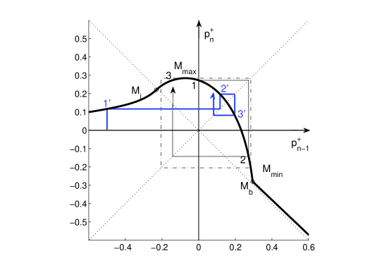
Figure 3: Graphical illustration of the iteration, where an initial point 1 is iterated into point 2, 3, etc. (similarly for the point 1’, 2’, 3’,…). Since the non-linear iteration function has a maximum $f_{max}$, after a few steps the iteration remains inside an “iteration square” shown in broken lines. This square has its upper side tangent to the maximum of the function, at point $M_{max}$, which after one iteration becomes point $M_{min}$ defining the lowest side of the square (ordinate $f_{min}$). Depending on the parameters, the iteration square contains or does not contain the contact point $M_{b}$ and the flow inversion point $M_{i}$. Here $\gamma=0.44$, $\zeta=0.8$, $\lambda=0.95$.

Singularities

An interesting feature of the iteration function is the discontinuity of its first derivative occurring at the beating limit point $M_{b}$ at $x=x_{b}$, given by:

$$x_{b}=\frac{1-\gamma}{2\lambda}\text{ \ \ \ ; \ \ \ }f(x_{b})=\frac{\gamma-1}{2}.$$ (17)

When the reed closes the channel ($p^{+}=p^{-}$, $p^{+}+p^{-}<\gamma-1$), $x>x_{b}$, $\ f(x)=-\lambda x$, the iteration function is linear.

Another singularity, i.e. a discontinuity of the second derivative, is obtained at the crossover between positive and negative flow, the inversion point $M_{i}$ where sign of the flow changes. Its abscissa $x=x_{i}$ is given by:

$$x_{i}=-\frac{\gamma}{2\lambda}\text{ \ \ \ ; \ \ \ }f(x_{i})=\frac{\gamma}{2}.$$ (18)

For $0<\gamma<1$, $x_{i}$ is negative and $x_{b}$ positive: therefore the initial point of the iteration ($x=0$) lies in the interval $\left[x_{i},x_{b}\right]$, with neither contact with the mouthpiece nor negative flow, as one could expect physically.

Schwarzian derivative

The Schwarzian derivative [3] of $f(x)$ is equal to:

$$Sf=\frac{f^{\prime\prime\prime}}{f^{\prime}}-\frac{3}{2}\left[\frac{f^{{}^{\prime\prime}}}{f^{\prime}}\right]^{2}\text{,}$$ (19)

where $f^{\prime}$, $f^{\prime\prime}$ and $f^{\prime\prime\prime}$ indicate the first, second and third derivatives of $f(x)$, respectively. If $x>x_{b}$, it is zero; if $x_{i}<x<x_{b}$, using the change of variables given in Appendix A, $Sf$ can be shown to be equal to:

$$Sf=\frac{8\lambda^{2}}{Y^{{}^{\prime}4}(Y^{\prime}-2)^{2}}\left[Y^{\prime\prime\prime}Y^{\prime}(Y^{\prime}-2)-3Y^{\prime\prime 2}(Y^{\prime}-1)\right],$$ (20)

where $Y$ is a function of $X$ - see Eqs. (27) to (A.1). Therefore its sign does not depend on the loss parameter $\lambda$. After some calculations, the Schwarzian derivative is found to be negative for all $x\in\left[x_{i},x_{b}\right]$ when $\zeta<1/\sqrt{5}.$ Otherwise, it is negative up to a certain value, then positive up to $x=x_{b}.$ The calculation of $Sf$ for the case $x<x_{i}$ shows that it is positive, except for a small interval. The iteration function therefore differs from a standard function because of the sign of the Schwartzian derivative; this is related to the nature of the bifurcation at the threshold of oscillation [23], which can be either direct or inverse.

Beating and negative flow limits

In Fig. 3 we see that, depending whether the contact point $M_{b}$  and flow inversion point $M_{i}$ of the iteration curve fall inside or outside the iteration square, a beating behavior of the reed and a sign inversion of the air flow are possible or not.

Point $M_{b}$ falls inside the iteration square if its abscissa $x_{b}$ given by (17) is smaller than $f_{max}$, which leads to:

$$\gamma>\gamma_{b}\equiv\frac{1-2\lambda A_{\zeta}}{1+\lambda}.$$ (21)

Figure 4: In the plane of the control parameters $\gamma$ and $\zeta$, the line representing $\gamma_{b}$ gives a border between the upper region, where reed beating may occur, and the lower region where it cannot - see Eq. (21). As a point of comparison, the line labelled $\gamma_{b2s}$ correspond to the limit obtained in [14] for the particular case of a 2-state regime, and given by Eq.(22). The figure also shows the line $\gamma_{i1}$ and $\gamma_{i2}$ associated with the possibility of negative flow (the first one turns out to be very close to that associated with reed beating). Small values for the losses have been assumed ($\lambda=0.95$).

The limiting value $\gamma_{b}$ is less than unity (it tends to $1/2$ when $\zeta$ tends to 0 and $\lambda$ tends to unity). This necessary condition is completely independent of the nature of the limit cycle, and less stringent than the limit $\gamma_{b2s}$ obtained in [14], for a 2-state cycle :

$$\gamma_{b2s}=1/2\left[1+\beta\beta_{1}+\beta_{1}^{2}(1-\beta\beta_{1})\right],$$ (22)

where $\beta=\zeta(1-\lambda)/(1+\lambda)$ and $\beta_{1}=\beta/\zeta^{2}.$ Fig. 4 gives a comparison between the two limits. Similarly, a necessary condition for possible inversions of the sign of the air flow is that point $M_{i}$ falls inside the iteration square of Fig 3, in other words that $x_{i}$ is larger than $f_{\min}$. We show in Appendix B that this happens if:

$$\gamma_{i1}<\gamma<\gamma_{i2}.$$ (23)

The expression of the two limits $\gamma_{i1}$ and $\gamma_{i2}$ are given in the Appendix and can be seen on Fig. 4.  They are solutions of $x_{i}=f_{\min}$, and exist only if the following condition holds:

$$\lambda>\frac{1}{1+2A_{\zeta}}.$$ (24)

Therefore, for a given $\zeta,$ negative flow is possible only above a certain value of $\lambda$; this value is $27/32=0.84$ for $\zeta=1$, and tends to unity when $\zeta$ tends to zero. Using a more realistic shape for the function $f(x)$ with a rounding of the kink at $x_{b}$ (no discontinuity of the derivative) should lead to a shorter range of negative flow, making the phenomenon even less likely, as illustrated in Fig. 4.

Of course, the two above conditions (21) and (23) are necessary, but not sufficient; they do not ensure that either beating or flow inversion will indeed take place, since this will be true only if the corresponding regions of the non-linear curve are reached during the iterations. Generally speaking, this will have more chance to occur in chaotic regimes, where many points are explored in the iterations, than in periodic regimes. Since no observation of negative flow has been reported in the literature, it is not clear whether this actually happens in real instruments.

In conclusion of this section, the iteration function is similar to those usually considered in the context of iterated maps, without really belonging to the category of “standard” functions. The major difference is actually the effect of the control parameters on the function, since usually the control parameters acts as a gain, expanding the vertical axis of the graph; here the parameter $\gamma$ (pressure in the mouth of the instrumentalist) translates the iteration function along an axis at $45^{\circ}$ of the coordinate axis, while the other control parameter $\zeta$ (the pressure of the lip on the reed) expands the function along the perpendicular axis. It is therefore not surprising that we should find a parameter dependence of the dynamical behaviors that is significantly different from the standard results.

4 Bifurcation curves

Figure 5 shows an example of bifurcation curves, for $\lambda=0.95$ and $\zeta=0.8$, and illustrates the relative complexity of the possible regimes. The upper curve corresponds to the outgoing amplitude $p^{+}$ (or $x$), the middle curve to acoustic pressure $p$, and the lower curve to the acoustic flow $u$. The three curves show the last 20 values obtained after computing 400 iterations for each value of the mouth pressure $\gamma$. By calculating $2000$ iterations for a given value of the parameter $\gamma$, we have checked that the limit cycle is then reached. Obviously this method leads to stable regimes only.

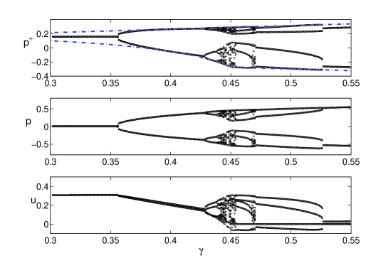
Figure 5: Bifurcation curve for $\lambda=0.95$ and $\zeta=0.8$. For increasing values of the abscissa $\gamma$ (blowing pressure), corresponding to a crescendo, the curve show the values after 400 iterations of the outcoming wave $p^{+}$ (top) the pressure $p$ in the mouthpiece (middle), and the volume flow $u$ (bottom). Above $\gamma\simeq 0.45$, the flow can be negative and the reed can beat. The top figure also shows $f_{\max}(\gamma)$ and $f_{\min}(\gamma)$ (mixed lines) associated to the “iteration square”.

When the control parameter $\gamma$ increases, the beginning of these curves follows a classical scenario of successive period doublings, leading eventually to chaos; as expected, high values of the parameters $\zeta$ and $\lambda$ favour the existence of chaotic regimes, as well as beating reed or negative flow. When $\gamma$ continues to increase, another phenomenon takes place: chaos disappears and is replaced by a reverse scenario containing a series of frequency (instead of period) doublings. We call this phenomenon a “backwards cascade” (in order to distinguish it from the usual “inverse cascade”, which takes place within periodicity windows inside chaos [2]); this backwards cascade is a consequence of the specificities of the effect of the control parameter on the iteration function in our model, and of the particular shape of the iteration function (for instance a straight line beyond the beating limit point). As a matter of fact, different kinds of cascades have been studied in the literature (see e.g. [24] and [25], in particular Fig.5).
In Fig. 5, the variations of $\gamma$ correspond to a “crescendo”: for a given value of $\gamma$, the initial value for the iteration, $p_{0}^{+}$, is chosen to be equal to the last value $p_{400}^{+}$ obtained with the previous value of $\gamma$. But we have also studied the “decrescendo” regime and observed that, in the chaotic regimes, the plotted points differ from the crescendo points; on the other hand, they remain the same in the periodic regimes, indicating a direct character of the bifurcations (no hysteresis). We have found an exception to this rule: between values $\gamma=0.5$ and $\gamma=0.53$, 2-state and 4-state regimes coexist, indicating an inverse bifurcation. Another inverse bifurcation, between a 2-state regime and a static regime, occurs beyond the limit of the figure, the two regimes coexisting between $\gamma=1$ and $\gamma=6.3544$; this is not shown here (the shape of the curve can be found in Ref. [14], see upper Fig. 4).

The two limits of the function $f(x)$, $f_{\max}$ and $f_{\min},$ are also plotted in the upper figure ( $p^{+}$) showing that, as expected, the corresponding values remain inside the iteration square (§ 3). In the figure at bottom, the results for the flow $u$ exhibit lower limits for negative flow and for beating, which are very close to the theoretical limits, respectively $\gamma_{i1}=0.4454$ and $\gamma_{b}=0.4503,$ and are located within the chaotic regime. Negative flow disappears at the bifurcation between the 4-state and the 2-state regime, $\gamma=0.5262$, a much lower value than the higher limit for negative flow $\gamma_{i2}=1.189$.

From $\gamma=$ Regime Comments From $\gamma=$ Regime Comments $0$ 1-state $0.4540$ 24-state $0.3545$ 2-state $0.4542$ 12-state $0.4272$ 4-state $0.4544$ 6-state $0.4384$ 8-state $0.466216$ I $0.4403$ 16-state $0.4664$ chaos $0.4408$ 32-state $0.46945$ 60-state $0.4409$ chaos $\gamma_{i1}=0.4454$ $0.4695$ 20-state $0.4467$ 6-state PW $0.4696$ chaos $0.4474$ 12-state PW $0.46985$ 4-state $0.4476$ 24-state PW $0.5000$ 2-state (D) $0.4479$ chaos $\gamma_{b}=0.4503$ $0.53$ 2-state (C) $0.4538$ 36-state $1.$ 1-state (D) $\gamma_{i2}=1.189$ $0.4539$ chaos $6.3544$ 1-state (C)

Table 1: Values of the parameter $\gamma$ at the lower limit of the different regimes, corresponding to Fig. 5. I=intermittencies; C= crescendo; D= decrescendo; PW= periodicity windows.

Table 1 shows the critical values of $\gamma$ corresponding to changes of regime. Up to the first chaotic regime ($\gamma=0.4409$), the behavior follows the usual period doubling cascade scenario. Between $\gamma=0.4467$ and $\gamma=0.4479$ a “periodicity windows” [2] is obtained, with 6-state, then 12-state and 24-state regimes (but no 3-state regime). Above the value $\gamma=0.4409$ for which chaos starts, an “inverse cascade” type scenario is observed, then intermittences occur, chaos again, and finally the “backwards cascade” to the static regime. We did not try to obtain the same accuracy for the values of all different thresholds, because the ranges for $\gamma$ have very different widths; for some values of $\gamma$, it has been necessary to make up to 2000 iterations, and sometimes it is not obvious to distinguish between a chaotic regime, a long transient, or an intermittency regime.

5 Iterated functions

We now discuss how the iterated functions can be used to study the different regimes and their stability. We write $f^{(2)}(x)$ the second iterate of $f$, and more generally $f^{(n)}(x)$ its iterate of order $n$; the derivative of $f$ with respect to $x$ is $f^{\prime}(x)$. Around the fixed point $x^{\ast}$ of the first iterate $f(x)$, a Taylor expansion gives:

$$f(x)=f(x^{\ast})+(x-x^{\ast})f^{\prime}(x^{\ast})+..=x^{\ast}+(x-x^{\ast})f^{\prime}(x^{\ast})+..\text{ \ \ ,}$$

which provides the well known stability condition for a fixed point $x^{\ast}$ of $f(x)$:

$$\left|f^{\prime}(x^{\ast})\right|<1.$$ (25)

Since the derivative of the iterate of order $n$ is given by:

$$f^{(n)\prime}(x^{\ast})=f^{\prime}(x^{\ast})f^{(n-1)\prime}(x^{\ast})$$

one can show by recurrence that, when $x=x^{\ast}$, it is equal to the $n$-th power of the derivative of $f$, so that:

$$f^{(n)}(x)=x^{\ast}+(x-x^{\ast})\left[f^{\prime}(x^{\ast})\right]^{n}+..$$ (26)

If the fixed point is stable (resp. unstable) with respect to $f(x)$, it is also stable (resp. unstable) with respect to any iterate. If $x$ is a vector, instead of a scalar, this linearized approach leads to the Floquet matrix, and $f^{\prime}(x)$ should be replaced by the eigenvalues of the matrix.

5.1 Stability of the period doubling regimes

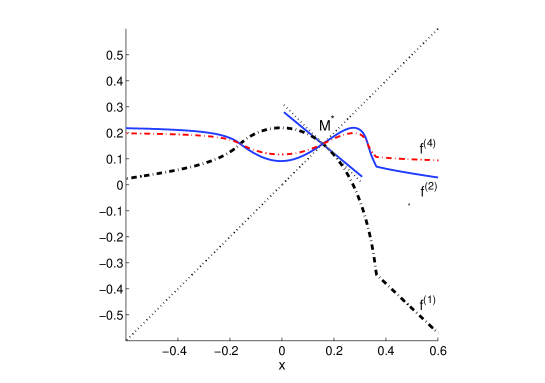
Figure 6: Iteration functions for $\lambda=0.95,$ $\ \gamma=0.31$ and $\zeta=0.8$. The 1st iterate $f(x)$ is shown with a mixed line, the 2nd iterate $f^{(2)}(x)$ with a (blue) solid line, and $f^{(4)}(x)$ with a (red), thin mixed line. The dotted lines are the first diagonal and the straight line perpendicular at the fixed point $M^{\ast}$ of $f(x)$, solution of $f(x)=x.$ The tangent lines to iterate 1 at the point $M^{\ast}$ is shown with a solid line.

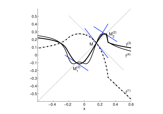
Figure 7: Iterates for $\lambda=0.95,$ $\ \gamma=0.42$ and $\zeta=0.8$, with the same plots that in figure 6. The tangent lines at the new fixed points of $f^{(2)}(x)$, $M_{1}^{(2)}$ and $M_{2}^{(2)}$, are also shown.

Examples of iterated functions of order 1, 2, and 4 are shown in figures 6 and 7, with the same values of $\zeta$ and $\lambda$ as in figure 5; in the former, the blowing pressure $\gamma$ is $0.31$, in the latter, $\gamma$ is $0.42$.  The first iterate has a unique fixed point, $M^{\ast}=(x^{\ast}$, $x^{\ast})$, located by definition on the first diagonal. The fixed point is stable if the absolute value of the derivative at $M^{\ast}$ is smaller than unity, in other words if the tangent line lies between the first diagonal (with slope $+1$) and its perpendicular (with slope $-1$). When $\gamma=$ $0.31$, we see in Fig. 6 that the fixed point $M^{\ast}$ is stable, so that no oscillation takes place. When $\gamma$ increases, M* becomes instable and, at the same time, gives rise to three fixed points of $f^{(2)}$.  For $\gamma=0.42$, Fig. 7 shows that the tangent is outside the angle between the diagonal and its perpendicular, so that the fixed point is now unstable; on the other hand, the second iterate $f^{(2)}$ now has two more fixed points $M_{1}^{(2)}$ and $M_{2}^{(2)}$ with slopes less than $1$ (in absolute value): we therefore have a stable 2-state regime.

The same scenario then repeats itself when $\gamma$ continues to increase: at some value, points $M_{1}^{(2)}$ and $M_{2}^{(2)}$ become instable in turn (the corresponding slope exceeds $1$ in absolute value), and both points $M_{1}^{(2)}$ and $M_{2}^{(2)}$ divide themselves into three fixed points of $f^{(4)}$; the two extreme new points have small slopes for this iterate, which leads to a 4-state stable regime. By the same process of successive division of fixed points of higher and higher iterates, one obtains an infinite number of period doublings, until eventually chaos is reached. This is the classical Feigenbaum route to chaos.

Some general remarks are useful to understand the shape of the iterates in the figures:

• If the value of $f(x)$ for the abscissa $x$ verifies $f(x)=f(x^{\ast})$, i.e. if the point $M$($x$, $f(x)$) is on a horizontal line $y=x^{\ast}$, all iterates go through the same point;

• The extrema of $f^{(2)}(x)$ verify either $f^{\prime}(x)=0$ (i.e. $x=x_{\max}$) or $f^{(2)}(x)=f_{\max}$ , because $df^{(2)}(x)/dx=f^{\prime}\left[f(x)\right]f^{\prime}(x)$; therefore the extrema of $f^{(2)}(x)$ are at either the same abscissa or the same ordinate as those of $f(x)$;

• More generally, for $n>1$, if $f^{(n-1)}(x)=x_{\max}$, then $f^{(n)}(x)=f_{\max}$, and it is at a maximum (its first derivative vanishes and the second one is negative), and if $f^{(n-1)}(x)=f_{\max}$, then $f^{(n)}(x)=f_{\min}$,  and it is at a minimum (its first derivative vanishes and the second one is positive);

• The kink of the first iterate (beating limit point) is also visible on the iterates;

• A well known property of the Schwarzian derivative is as follows : If the Schwarzian derivative of $f(x)$ is negative, the Schwarzian derivatives of all iterates are negative as well.

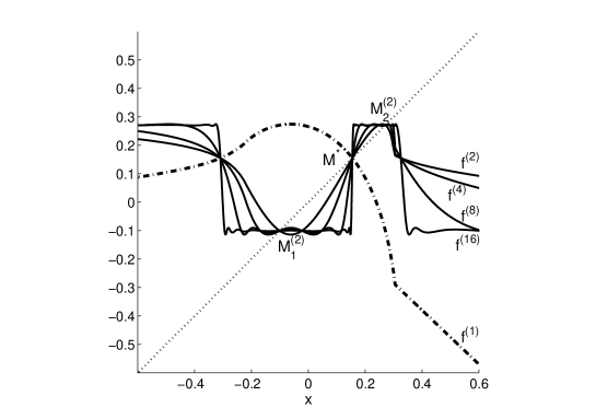
Figure 8: Iterates for $\lambda=0.95,$ $\ \gamma=0.42$ and $\zeta=0.8$, of order 1, 2, 4, 8 and 16. The convergence to the 2-state regime is visible.

Figure 8 shows the higher order iterates (of order 4, 8 and 16) in the same conditions as figure 7. We observe that the iterates become increasingly close together when their order increases, with smaller and smaller slopes at the fixed points corresponding to the 2-state regime. Moreover, they resemble more and more a square function, constant in various domains of the variable. This was expected: in the limit of very large orders, whatever the variable is (i.e. whatever the initial conditions of the iteration are) one reaches a regime where only two values of the outgoing wave amplitude are possible; these values then remain stable, meaning that the action of more iterations will not change them anymore. So, one can read directly that the limit cycle is a 2-state on the shape of $f^{16}$, which has two values; it would for instance have 4 in the limit cycle was a 4-state regime for these values of the parameters. For the clarity of the figure, we have shown only iterates with orders that are powers of $2$, but it is of course easy to plot all iterates. For a 2-state regime, even orders are sufficient to understand the essence of the phenomenon, since odd order iterates merely exchange the two fixed points $M_{1}^{(2)}$ and $M_{2}^{(2)}$.

In table 1, the existence of two different stable regimes for the same value of the parameters signals an inverse bifurcation; Figure 9 shows an example of such a situation. For $\gamma=1.2$, both the static and 2-state regimes are then stable, depending on the initial conditions. For the static regime, the curve $f^{(1)}$ coincides with the second diagonal $y=-x$, a case in which the fixed point is presumably stable (the stability becomes intuitive when one notices that the tangents of the higher order curves lie within the angle of the two diagonals). For the 2-state regime, the state of positive pressure value corresponds to a beating reed.

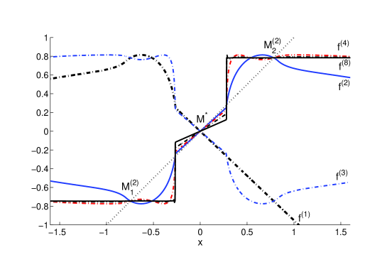
Figure 9: Iterates for $\lambda=0.95,$ $\ \gamma=1.5$ and $\zeta=0.8$, of order 1, 2, 3, 4, and 8. The curves of $f^{(8)}$ and $f^{(16)}$ are almost perfectly superimposed. Around $x=0$, the convergence to the static regime appears to be very slow. On the contrary the convergence to the 2-state regime is rapid.

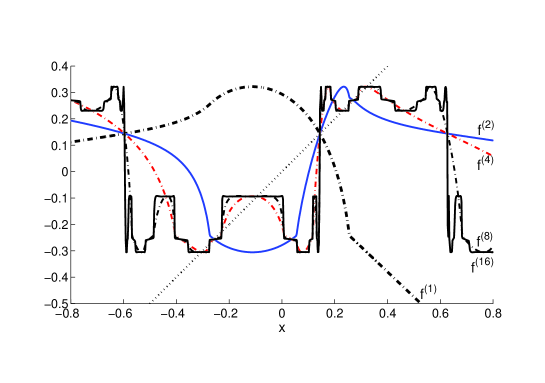
Figure 10: Iterates for $\lambda=0.95,$ $\ \gamma=0.515$ and $\zeta=0.8$, of order 1, 2, 4, 8 and 16.

Finally Fig.10 shows another case of existence of two different regimes for the same value of the parameters. A 2-state regime can occur, as well as a 4-state regimes can occur. It appears that the second one is more probable than the first one, when initial conditions are varied.

5.2 Periodicity windows; intermittencies

We now investigate some regimes occurring in a narrow range of excitation parameter $\gamma$.

(i) We first examine a chaotic regime occurring just before a 6-state regime (period tripling) and the transition between the two regimes. Figure 11 shows the iterated functions of order 1, 2, 6, and 12. The 6th iterated function crosses the first diagonal at the same points than the first and the second iterates only, which means that no 6-state regime is expected. By contrast, the 12th iterate cuts the diagonal at more points, but with a very high slope, indicating that the corresponding fixed points cannot be stable. This, combined with the fact that no convergence to a square function (constant by domains), such as $f^{16}$ in Figure 8, suggests an aperiodic behavior; the time dependent signal shown in Fig.12 looks indeed chaotic (nevertheless the flow always remains positive). The periodic/chaotic character of the signal can be distinguished by examining the time series, but a complementary method is the computation of an FFT. For the signal of Fig.12, the spectrum is more regular than the spectrum of a 6-state periodic regime. Nevertheless the frequencies of the latter (the “normal” frequency $f_{2}$ of the 2-state regime with the frequencies $f_{2}/3$ and $2f_{2}/3$) remains visible in the spectrum of the first one, as it is often the case for signals corresponding to very close values of the parameter. A consequence is that these frequencies clearly appear when listening the sound.

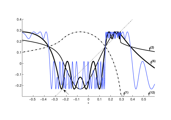
Figure 11: Iterates for $\lambda=0.95,$ $\ \gamma=0.4445$ and $\zeta=0.8$, of order 1, 2, 6 and 12. A convergence to an aperiodic regime is visible. The arrow indicates a region where $f^{(6)}(x)$ is very close to the first diagonal, but does not yet cross it.

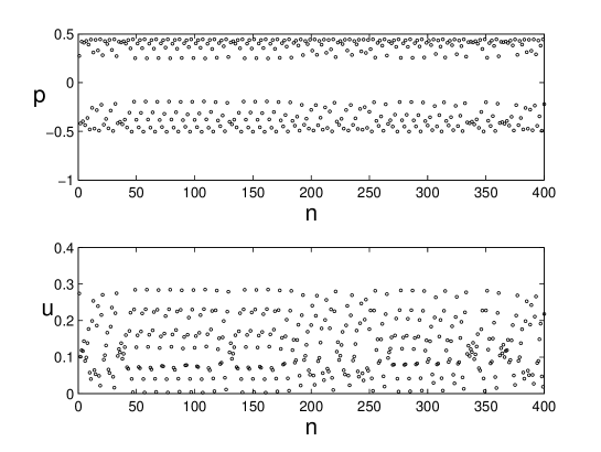
Figure 12: Iteration from $n=0$ for $\lambda=0.95,$ $\zeta=0.8$, $\gamma=0.4445$, $p_{0}^{+}=0$; the upper part shows the the pressure $p$, the lowest part the values of the flow $u$. The regime looks chaotic.

Figure 13 is similar to figure 11, but with a slightly larger value of $\gamma$ ($0.4469$ instead of $0.4445$). In the region indicated by the arrow, one notices that the 6th iterated function now cuts the first diagonal. They are 12 points of intersection (plus 1 common point with the first iterate as well as two common points with the second iterate, all unstable); the slope of the tangent shows that 6 of them are stable, so that one obtains a 6-state, periodic, regime. The variations of higher order iterates, e.g. $f^{(12)}$, remain very fast; the convergence to the limit cycle is then much slower than for Fig. 8, except if the initial point is close to a limit point (e.g. that shown by an arrow: it turns out that the 12th iterated function is very close to the 6th one). As a consequence, the initial transient to the 6-state regime can be rather chaotic, as shown in Fig. 14, but convergence to a periodic regime does occur later. This existence of periodic regimes above the threshold for chaos is called “periodicity windows”, which appears as a narrow whiter region in Fig. 5. A difference with the usual $2^{n}$-state regimes (when $\gamma$ is below the chaotic range), for instance corresponding to Fig. 7, is that one obtains $2^{n}$ intersections with the diagonal, stable or unstable; by contrast, for the 6-state regime, they are 6 stable and 6 unstable points.

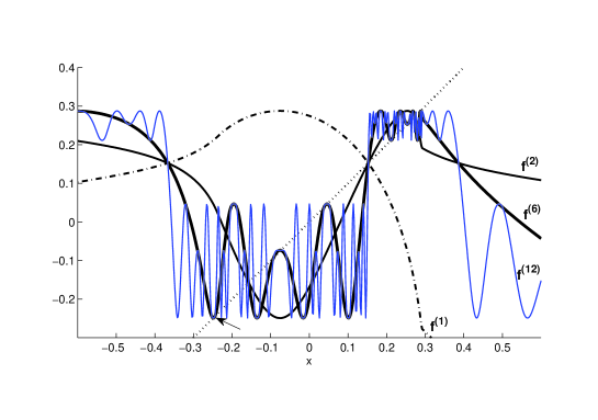
Figure 13: Iterates for $\lambda=0.95,$ $\ \gamma=0.4469$ and $\zeta=0.8$, of order 1, 2, 6 and 12. A convergence to a 6-state regime is observed. The arrow indicates a region where $f^{(6)}(x)$ cuts the first diagonal.

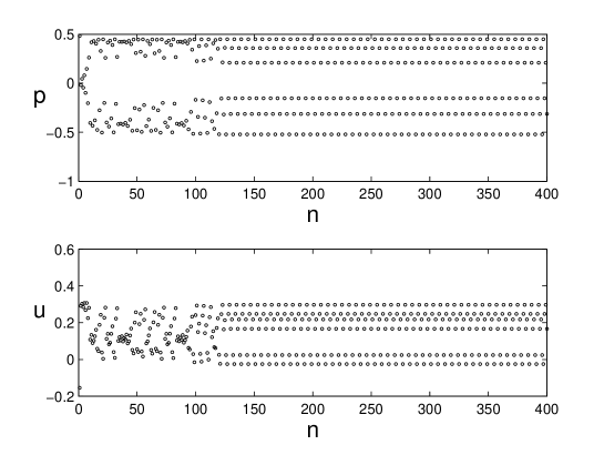
Figure 14: Iteration from $n=0$ for $\lambda=0.95,$ $\zeta=0.8$, $\gamma=0.4469$, $p_{0}^{+}=-0.3347.$ The regime is periodic (6-state).

(ii) We now examine the transition between a 6-state regime and a 4-state regime through chaotic regimes or intermittency regimes. For $\gamma=0.4544$, a 6-state regime is obtained. Fig. 15 shows the iterates of order 1, 2, 4 and 6. The 4th and 6th iterates have common intersections with the first and second iterates, since both 4 and 6 are multiples of 2. The 6th iterate intersects the first diagonal at 12 other points, while the 4th cuts the diagonal at 4 points only. These 4 points are unstable, thus no 4-state regime can exist. On the contrary, for the 6th iterate, half of the 12 points are stable (i.e. with a small slope of the tangent line), so that one obtains a 6-state stable regime.

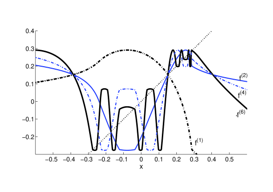
Figure 15: Iterates for $\lambda=0.95,$ $\ \gamma=0.4544$ and $\zeta=0.8$, of order 1, 2, 4 and 6. A convergence to a 6-state regime is observed.

What happens for a higher value of $\gamma,$ namely $0.472$ corresponding to a 4-state regime is shown in Fig. 16, with again the iterates of order 1, 2, 4, 6. The 4th iterate curve crosses the diagonal for the same number of points than previously, but the 4 points are now stable. The 6th order iterate does not intersect the diagonal, except at the common points with the two first iterates.

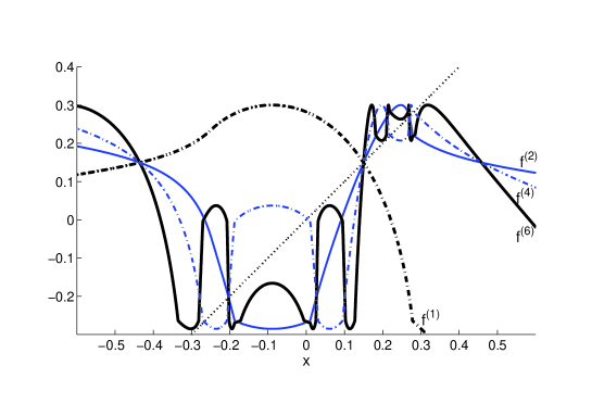
Figure 16: Iterates for $\lambda=0.95,$ $\ \gamma=0.472$ and $\zeta=0.8$, of order 1, 2, 4 and 6. A convergence to a 4-state regime is observed.

Between the two preceding values of the parameter $\gamma$, both chaotic and intermittent regimes can exist. For $\gamma=0.46623$, Figure 17 shows intermittencies between a chaotic and a 6-state behaviors (upper curve), and Figure 18 shows that the 6th iterate is tangent to the first diagonal in 6 points, so that the resulting permanent regime can be interpreted as a kind of “hesitation” between two behaviors. The 4 intersections of the 4th iterate remain unstable.
The lower curve in Figure 17 shows another, more visible, example of intermittencies, obtained with slightly different values of the parameters, between a chaotic regime and a 4-state one (actually it is a 8-state one, very close to a 4-state regime).

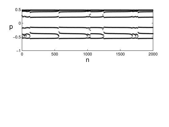
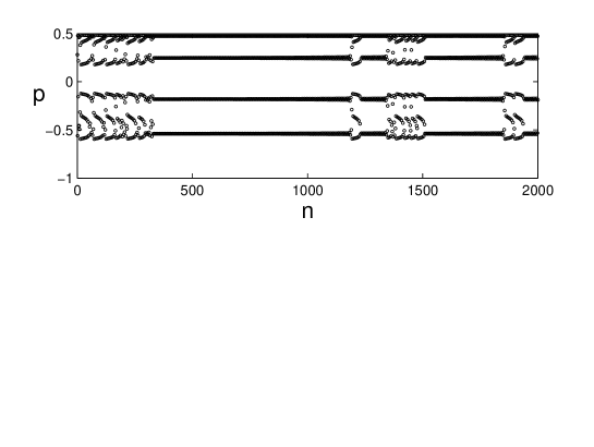
Figure 17: Iteration from $n=0$ for $\lambda=0.95,$ $\zeta=0.8$, $\gamma=0.46623,$ $p_{0}^{+}=0$ (upper curve): Intermittencies between chaos and a 6-state regime are observed. However the lower curve (for $\lambda=1,$ $\zeta=0.8$, $\gamma=0.467,$ $p_{0}^{+}=0$) shows a more clear situation of intermittencies between chaos and a 4-state regime.

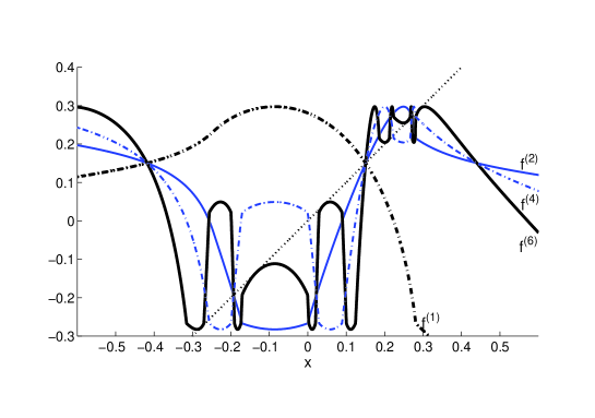
Figure 18: Iterates for $\lambda=0.95,$ $\ \gamma=0.46623$ and $\zeta=0.8$, of order 1, 2, 4 and 6, corresponding to intermittencies. The sixth iterate is tangent to the diagonal.

6 Conclusion

The study of the iteration model of the clarinet should not be limited to the first iterate: higher order iterates give interesting information on possible regimes of oscillation. In the limit of very high orders, their shape gives a direct indication of the number of states involved in the limit regime, or of chaotic behavior. One can also predict an intermittent regime of the iterations, which takes place when an iterate is almost tangent to the first diagonal, so that the iterations are “trapped” for some time in a narrow channel. The phenomenon might be related to some kinds of multiphonic sounds produced by the instrument. It is true that this phenomenon takes place only in a rather narrow domain of parameters, but this is also the case of the period doubling cascade, which has been observed experimentally. One can therefore reasonably hope that the present calculations will be followed by experimental observations.

Appendix A Analytical iteration function

A.1 Derivation of the equations

Our purpose is to obtain an analytical expression of the iteration function $p_{n}^{+}=f(p_{n-1}^{+}).$ From the basic model (Eqs. (2.1 to 2.1, 7, 11)), the following quantities can be defined:

$$\text{ }X = \gamma-p_{n}=\gamma-p_{n}^{+}-p_{n}^{-}=\gamma-p_{n}^{+}+\lambda p_{n-1}^{+}\text{\ ; }$$

$$\text{\ }Y = u_{n}+X=\gamma-2p_{n}^{-}=\gamma+2\lambda p_{n-1}^{+}\text{.}$$

$p_{n}^{+}=g($ $p_{n}^{\_})$ can be obtained from the knowledge of the function $X(Y),$ given by the solving of:

$$Y=X\text{ \ (beating reed, }X>1\text{);}$$ (27)

$$Y = X+\zeta(1-X)\sqrt{X}\text{\ (non-beating }$$

$$\text{reed, positive flow, }0<X<1\text{);}$$

$$Y = X-\zeta(1-X)\sqrt{-X}\text{ \ \ (non-beating }$$

$$\text{reed, negative flow, }X<0\text{).}$$

For the non-beating reed case, the study of function $Y(X)$ leads to a direct analytical solution, as explained below, at least if $\zeta<1$ (otherwise it is a multi-valued function).

Finally, with the notation $x=p_{n-1}^{+}$ and $f(x)=p_{n}^{+}$, if $\mathcal{Y}(X)$ is the Heaviside function, the iteration function is obtained, as:

$$f(x) = \gamma-X(Y)+\lambda x\text{, with }Y=\gamma+2\lambda x\text{ and}$$ (30)

$$Y(X) = X+\zeta sign(X)\,\mathcal{Y}(1-X)(1-X)\sqrt{\left|X\right|}.$$ (31)

A.2 Non-beating reed, positive flow  (0$\leq Y\leq 1)$

For this case, both $X$ and$\ Y$  are positive and smaller than unity, because $\zeta<1.$ Writing $Z=\sqrt{X}$, Eq. (A.1) is written as:

$$G_{1}(Z)=Y\text{, \ \ where }G_{1}(Z)=-\zeta Z\left[Z^{2}-\frac{Z}{\zeta}-1\right].$$ (32)

The study of function $G_{1}(Z)$ shows that it is monotonously increasing from $0$ to $1$ when $Z$ increases from $0$ to $1.$ Therefore the equation $G_{1}(Z)=Y$ has a unique solution when $0\leq Y\leq 1.$ With this condition, it appears that the equation has three real solutions, and that the interesting solution (located between $0$ and $1$) is the intermediate one. As a conclusion, it is possible to use the classical formula for the solution of the cubic equation:

$$\sqrt{X} = Z=-\frac{2}{3}\eta\sin\left[\frac{1}{3}\arcsin\left(\frac{\psi-\mu}{\zeta\eta^{3}}\right)\right]+\frac{1}{3\zeta}\text{ \ ;}$$

$$\psi = \frac{1}{\zeta^{2}}\text{ ; }\eta=\sqrt{3+\psi}\text{ ; }\mu=\frac{9}{2}(3Y-1).$$

A.3 Non-beating reed, negative flow (Y$\leq 0)$

For this case, both $X$ and$\ Y$  are negative. Writing $Z=\sqrt{-X}$, Eq. (A.1) is written as follows:

$$G_{2}(Z)=Y\text{, where }G_{2}(Z)=-\zeta Z\left[Z^{2}+\frac{Z}{\zeta}+1\right].$$ (33)

The study of the function $G_{2}(Z)$ shows that it is monotonously decreasing from $0$ when $Z$ increases from $0.$ Therefore the equation $G_{2}(Z)=Y$ has a unique real, positive solution when $Y\leq 0.$ The two other solutions are either real and negative or complex conjugate, with a negative real part, because the sum of the three solutions is negative ($-1/\zeta$). As a conclusion, the solution can be written by using the following formulae:

If the discriminant is positive

$$discr=q^{3}+r^{2}>0\text{, where}$$

$$q = \frac{1}{9}\left[3-\psi\right]\text{ \ ; }r=-\frac{\psi+\mu}{27\zeta}\text{ }.$$

$$\sqrt{-X} = Z=s_{1}-\frac{q}{s_{1}}-\frac{1}{3\zeta}\text{; }s_{1}=\left[r+\sqrt{discr}\right]^{1/3}.$$

If the discriminant is negative

$$discr=q^{3}+r^{2}<0$$

$$\sqrt{-X} = Z=\frac{2}{3}\eta^{\prime}\cos\left[\frac{1}{3}\arccos\left(-\frac{\psi+\mu}{\zeta\eta^{\prime 3}}\right)\right]-\frac{1}{3\zeta}\text{ ;}$$

$$\eta^{\prime} = \sqrt{-3+\psi}.$$

Appendix B Negative flow limit

The condition of existence of negative flow is given by $x_{i}>f_{\min}$. This is equivalent to the condition on the antecedents, $x_{i}^{\prime}<f_{\max}$, where $x_{i}^{\prime}$ is the larger antecedent of $x_{i}$, such as $x_{i}^{\prime}>x_{\max},$ because $f(x)$ is decreasing for all $x>x_{\max}$ (see Fig. 2). Therefore the volume flow is negative at time $n+1$.

In order to determine the limit value $\gamma_{i}$, the following equations are to be used:

$$X = \gamma-x_{i}+\lambda x_{i}^{\prime}\text{ }=\frac{\gamma}{2\lambda}(1+\lambda)^{2}+\lambda A_{\zeta}\text{\ ; }$$ (34)

$$Y = \gamma+2\lambda x_{i}^{\prime}=\gamma(1+\lambda)+\lambda 2A_{\zeta}.$$ (35)

$\gamma$ being positive (a reasonable hypothesis for the normal playing), the unknown $X$ needs to be larger than the quantity $\lambda A_{\zeta}.$ Eliminating $\gamma$ in the above equations implies the following equation, with $X>\lambda A_{\zeta}$:

$$Y(X)-X=\frac{(\lambda-1)X+2\lambda A_{\zeta}}{1+\lambda},$$

or

$$H(X)=\delta\text{ \ ,}$$ (36)

with:

$$H(X) = (1+\lambda)\left[Y(X)-X\right]+(1-\lambda)X\text{ \ }$$ (37)

$$\text{for\ \ }X > \lambda A_{\zeta}\text{ \ \ ; \ \ }\delta=2\lambda A_{\zeta}.$$

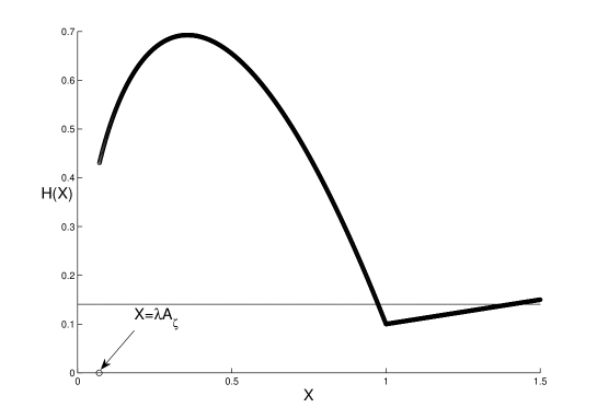
Figure 19: Function $H(X)$ given by Eq. (37) and constant line $\delta=2\lambda A_{\zeta}.$ Two solutions $X>\lambda A_{\zeta}$ exits for this case ($\lambda=0.9$, $\zeta=0.9$), because condition (24) is satisfied.

An example of function $H(X)$ is shown in Fig. 19. It appears that no solutions exist if $H(1)>\delta$ and two solutions exist if $H(1)<\delta$, i.e. if inequation (24) holds. The two solutions can be obtained analytically. However, for sake of simplicity, we give the exact solution for the larger one, $\gamma_{i2}$, and an approximation for the smaller one, $\gamma_{i1}$, obtained at the first order in $\varepsilon=1-X$:

$$\gamma_{i2} = \frac{2\lambda^{2}A_{\zeta}}{1-\lambda^{2}}\text{;}$$ (38)

$$\gamma_{i1} \simeq \frac{2\lambda}{(1+\lambda)^{2}}\left[1-\lambda A_{\zeta}-\varepsilon\right]\text{,}$$ (40)

$$\text{ with }\varepsilon=\frac{\lambda-1+2\lambda A_{\zeta}}{(\lambda+1)\zeta+\lambda-1}.$$

This error is found to be less than $1\%$ in comparison with the exact value. Condition (24)

can be shown to be necessary and sufficient. We do not give the entire proof, but it can be shown that another necessary condition for having two solutions is $H^{\prime}(1^{-})<0$, or  $\zeta(\lambda+1)+\lambda-1>0$, but it is implied by condition (24)

.

Fig. 4 shows that the first negative flow threshold $\gamma_{i1}$ is very close to the threshold $\gamma_{b}$, and slightly smaller. For a given $\lambda$, the limit value of $\zeta$ such as $\lambda>1/(1+2A_{\zeta})$ corresponds to the equality between the beating reed threshold and the negative flow one. For a given $\zeta,$ negative flow is possible above a certain value of $\lambda$. For rather strong losses, if $\lambda<0.84$, no negative flow can occur. For a cylindrical resonator, this implies that $\alpha\ell>0.085$.

References

- [1] May, R. M., “Simple mathematical models with very complicated dynamics”, Nature 261, 1976, 459-67.
- [2] Bergé, P. , Pomeau, Y. and Vidal, C., Order within chaos, Hermann and Wiley, UK, 1986; L’ordre dans le chaos, Hermann, Paris, 1984.
- [3] Collet, P. and Eckmann, J.P. , “Properties of Continuous Maps of the Interval to Itself”, Mathematical Problems in Theoretical Physics, K. Osterwalder (ed.), Springer-Verlag, Heidelberg, 1979; Iterated Maps on the Interval as Dynamical Systems, Birkhäuser, Basel, 1980.
- [4] Feigenbaum, J., “The Universal Metric Properties of Nonlinear Transformations”. Journal of Statistical Physics, 21, 1979, 669-706; “The metric universal properties of period doubling bifurcations and the spectrum for a route to turbulence”, Annals of the New York Academy of Science, 357, 1980, 330-336.
- [5] McIntyre, M. E. , Schumacher, R. T., and Woodhouse, J. . On the oscillations of musical instruments. Journal of the Acoustical Society of America, 74, 1983, 1325–1345.
-
[6]
Maganza, C., Caussé, R. and Laloë, F. .
“Bifurcations, period doubling and chaos in clarinetlike systems”, Europhysics letters 1, 1986, 295–302.
- [7] Brod, K., “Die Klarinette als Verzweigungssytem : eine Anwendung der Methode des iterierten Abbildungen”. Acustica, 72, 1990, 72–78.
- [8] Kergomard, J., “Elementary considerations on reed-instrument oscillations”. In Mechanics of musical instruments, vol. 335 (A. Hirschberg/ J. Kergomard/ G. Weinreich, eds),of CISM Courses and Lectures, pages 229–290. Springer-Verlag, Wien, 1995.
- [9] Lizée, A., Doublement de période dans les instruments à anche simple de type clarinette, Master degree thesis, Paris 2004, http://www.atiam.ircam.fr/Archives/Stages0304/lizee.pdf
- [10] Idogawa, T. , Kobata, T. , Komuro, K. and Masakazu, I., “Nonlinear vibrations in the air column of a clarinet artificially blown”, Journal of the Acoustical Society of America, 93, 1993, 540–551.
- [11] Gibiat, V. and Castellengo, M. . “Period doubling occurences in wind instrument musical performances”, Acustica united with acta acustica, 86, 2000, 746–754.
- [12] Kergomard, J., Dalmont, J.P. , Gilbert, J. and Guillemain, Ph. . “Period doubling on cylindrical reed instruments”. In Proceedings ot the Joint congress CFA/DAGA’04, pages 113–114, Strasbourg, 22th 25th March 2004.
- [13] Ollivier, S. , Kergomard, J. and Dalmont, J.-P. “Idealized models of reed woodwinds. Part II: On the Stability of ”Two-Step” Oscillations”. Acta Acustica united with Acustica, 91, 2005, 166–179.
- [14] Dalmont, J.-P. , Gilbert, J., Kergomard, J. and Ollivier, S. “An analytical prediction of the oscillation and extinction thresholds of a clarinet”. Journal of the Acoustical Society of America, 118, 2005, 3294–3305.
- [15] Vallée, R. and Delisle, C. , “Periodicity windows in a dynamical system with delayed feedback”, Physical Review A, 34, 1986, 309-3018.
- [16] Stefanski, K., “Universality of succession of periodic windows in families of 1D-maps”. Open Systems & Information Dynamics, 6, 1999, 309-324.
- [17] Wilson, T.A. and Beavers, G.S. , “Operating modes of the clarinet”. Journal of the Acoustical Society of America, 56, 1974, 653-658.
- [18] Hirschberg, A. , Van de Laar, R. W. A. , Marrou-Maurires, J. P. , Wijnands, A. P. J., Dane, H. J. , Kruijswijk, S. G. and Houtsma, A. J. M. “A Quasi-stationary Model of Air Flow in the Reed Channel of Single-reed Woodwind Instruments”. Acustica, 70, 1990, 146–154.
- [19] Dalmont, J.-P., Gilbert, J. and Ollivier, S. . “Nonlinear characteristics of single-reed instruments: quasistatic volume flow and reed opening measurements”, Journal of the Acoustical Society of America, 114, 2003, 2253–2262.
- [20] Dalmont, J.-P. and Frappé, C.,“ Oscillation and extinction thresholds of the clarinet: Comparison of analytical results and experiments”. Journal of the Acoustical Society of America, 122, 2007, 1173–1179.
- [21] Caussé, R., Kergomard, J., Lurton, X., “Input impedance of brass musical instruments - comparison between experiment and numerical model”, Journal of the Acoustical Society of America, 75, 1984, 241-254.
- [22] Raman, C.V., “On the mechanical theory of vibrations of bowed strings [etc.]”. Indian Association for the Cultivation of Science Bulletin, 15, 1918, 1–158.
- [23] Mayer-Kress, G. and Haken, H. , “Attractors of convex maps with positive Schwarzian derivative in the presence of noise”, Physica 10D, 1984, 329-339.
- [24] Parlitz, U., Englisch, V., Scheffczyk, C. and Lauterborn, W., “Bifurcation structure of bubble oscillators”, Journal of the Acoustical Society of America, 88, 1990, 1061-1077.
- [25] Scheffczyk, C., Parlitz, U., Kurz, T., Knop, W., Lauterborn, W., “Comparison of bifurcation structures of driven dissipative nonlinear oscillators”,Physical Review A, 43, 1991, 6495-6502.