X-ray Radiation Mechanisms and Beaming Effect of Hot Spots and Knots in Active Galactic Nuclear Jets

Abstract

The observed radio-optical-X-ray spectral energy distributions (SEDs) of 22 hot spots and 45 knots in the jets of 35 active galactic nuclei are complied from literature and modeled with single-zone lepton models. It is found that the observed luminosities at 5 GHz ($L_{\rm 5GHz}$) and at 1 keV ($L_{\rm 1keV}$) are tightly correlated, and the two kinds of sources can be roughly separated with a division of $L_{\rm 1keV}=L_{\rm 5GHz}$. Our SED fits show that the mechanisms of the X-rays are diverse. While the X-ray emission of a small fraction of the sources is a simple extrapolation of the synchrotron radiation for the radio-to-optical emission, an inverse Compton (IC) scattering component is necessary to model the X-rays for most of the sources. Considering the sources at rest (the Doppler factor $\delta=1$), the synchrotron-self-Compton (SSC) scattering would dominate the IC process. This model can interpret the X-rays of some hot spots with a magnetic field strength ($B_{\rm ssc}^{\delta=1}$) being consistent with the equipartition magnetic field ($B_{\rm eq}^{\delta=1}$) in one order of magnitude, but an unreasonably low $B_{\rm ssc}^{\delta=1}$ is required to model the X-rays for all knots. Measuring the deviation between $B_{\rm ssc}^{\delta=1}$ and $B_{\rm eq}^{\delta=1}$ with ratio $R_{B}\equiv B_{\rm eq}^{\delta=1}/B_{\rm ssc}^{\delta=1}$, we find that $R_{B}$ is greater than 1 and it is tightly anti-correlated with ratio $R_{L}\equiv L_{\rm 1keV}/L_{\rm 5GHz}$ for both the knots and the hot spots. We propose that the deviation may be due to the neglect of the relativistic bulk motion for these sources. Considering this effect, the IC/CMB component would dominate the IC process. We show that the IC/CMB model well explains the X-ray emission for most sources under the equipartition condition. Although the derived beaming factor ($\delta$) and co-moving equipartition magnetic field ($B_{\rm eq}^{{}^{\prime}}$) of some hot spots are comparable to the knots, the $\delta$ values of the hot spots tend to be smaller and their $B_{\rm eq}^{{}^{\prime}}$ values tend to be larger than that of the knots, favoring the idea that the hot spots are jet termination and knots are a part of a well-collimated jet. Both $B_{eq}^{{}^{\prime}}$ and $\delta$ are tentatively correlated with $R_{L}$. Corrected by the beaming effect, the $L^{{}^{\prime}}_{\rm 5GHz}-L^{{}^{\prime}}_{\rm 1keV}$ relations for the two kinds of sources are even tighter than the observed ones. These facts suggest that, under the equipartition condition, the observational differences of the X-rays from the knots and hot spots may be mainly due the differences on the Doppler boosting effect and the co-moving magnetic field of the two kinds of sources. Our IC scattering models predict a prominent GeV-TeV component in the SEDs for some sources, which are detectable with H.E.S.S. and Fermi/LAT.

1 Introduction

Hot spots and knots in large-scale jets have been observed in many active galactic nuclei (AGNs). Hot spots are often found near the outmost boundaries of radio lobes. They are regarded as jet termination (Fnanaroff & Riley 1974; Blandford & Rees 1974; Begelman et al. 1984; Bicknell 1985; Meisenheimer et al. 1989). Knots are usually thought to be a part of a well-collimated jet (e.g., Harris & Krawczynski 2006). Some of them are also detected in the optical and X-ray bands. With high spatial resolution and sensitivity, the Chandra X-ray Observatory opened a new era to study the X-ray emission of hot spots and knots. It revealed that bright radio knots and hot spots in radio galaxies and quasars are also often detected in the X-ray band (Wilson et al. 2001; Hardcastle et al. 2004; Kataoka & Stawarz 2005; Tavecchio et al. 2005).

The X-ray radiation mechanisms of hot spots and knots are highly debated. It is generally believed that synchrotron radiation of relativistic electrons is responsible for the radio emission. The detection of high polarization in the optical emission indicates that the optical emission is also from synchrotron radiation (Roser & Meisenheimer 1987; Lähteenmäki & Valtaoja 1999). It is uncertain whether the X-ray emission is a simple extrapolation of the synchrotron radiation for the radio-to-optical emission. Indeed, the X-rays of some hot spots (such as hot spots N1 and N2 in 3C 33; Kraft et al. 2007) and knots (such as the knots in 3C 371 and M87; Sambruna et al. 2007; Liu & Shen 2007) can be interpreted as synchrotron radiation from the same electron population responsible for the radio and optical emission. However, the X-ray emission of some hot spots and knots is apparently not a simple extrapolation of the radio-to-optical component (Kataoka & Stawarz 2005). An inverse Compton scattering (IC) component is necessary to model the X-rays. As shown by Stawarz et al. (2007), the X-ray emission of hot spots in Cygnus A is well interpreted with the synchrotron-self-Compton (SSC) scattering model. The IC scattering of cosmic microwave background (IC/CMB) may also significantly contribute to the observed X-ray emission, if the bulk flow of the material in hot spots and knots is relativistic (Georganopoulos & Kazanas 2003).

Broadband spectral energy distribution (SED) places strong constraints on the radiation mechanism models. Systematical analysis on the SEDs in the radio and X-ray bands of hot spots, knots and lobes were present by Hardcastle et al. (2004) and Kataoka & Stawarz (2005). Note that the optical data are critical to characterize the SEDs, and may give more constraints on the models. In this paper, we compile a large sample of the observed SEDs in the radio-optical-X-ray band of hot spots and knots from literature, and fit them with various models in order to study the radiation mechanisms of the X-rays and to reveal the differences of the two kinds of sources.

The magnetic field and Doppler boosting effect are crucial ingredients in SED modeling. The energy equipartition assumption between magnetic field and radiating electrons is usually accepted in discussion of the energetics and dynamics of radio sources. Hardcastle et al. (2004) reported that most radio-luminous hot spots can be explained with the SSC model under this assumption. With the equipartition condition, the derived magnetic field of lobes is $\sim 10^{-6}$G (Kataoka & Stawarz 2005), being comparable to the strength of the magnetic field in the interstellar medium. Since hot spots are believed to be the terminal of a relativistic jet, the Doppler boosting effect would be less prominent than that in knots, but their magnetic fields may be magnified up to $\sim 10^{-4}$G by strong external shocks produced by interaction of a relativistic jet with circum medium (Kataoka & Stawarz 2005). Therefore, the Doppler boosting effect and co-moving magnetic field are essential to discriminate the two kinds of sources, if they are physically different. With our detailed SED fits, we compare their Doppler factor ($\delta$) and co-moving magnetic field ($B^{{}^{\prime}}$) between the knots and hot spots in our sample under the equipartition assumption.

The observed SEDs and our data analysis are present in §2. Models and our SED fits are shown in §3. Conclusions and discussion are present in §4. Throughout, $H_{0}$=70 km s^-1 Mpc^-1, $\Omega_{\Lambda}=0.7$ and $\Omega_{m}=0.3$ are adopted.

2 Sample and Data Analysis

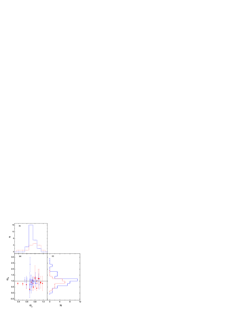
Figure 2: Distributions of the observed spectral indices in the radio and X-ray bands for the knots (circles/solid lines) and hot spots (squares/dashed lines).

Twenty-two hot spots and 45 knots from 35 AGNs (15 radio galaxies, 16 quasars, 3 BL Lac objects, and 1 Seyfert galaxy; see Table 1) are included in our sample. Most of them are taken from XJET Home Page. Observations for these hot spots and knots are summarized in Table 2, and their SEDs are displayed in Figure 1. We show the distributions and the correlations of the spectral indices in the radio and X-ray bands ($\alpha_{r}$ and $\alpha_{X}$) in Figure 2. It is found that $\alpha_{r}$ is not correlated with $\alpha_{X}$. The $\alpha_{r}$ of both the knots and hot spots are smaller than 1. The $\alpha_{X}$ narrowly clusters at $0.7\sim 1.2$ for the hot spots, but it ranges in $0.2\sim 2.4$ for the knots. We test whether $\alpha_{r}$ and $\alpha_{X}$ distributions show statistical differences between the two kinds of sources with the Kolmogorov-Smirnov test (K-S test), which yields a chance probability $p_{\rm KS}$. A K-S test probability larger than 0.1 would strongly suggest no statistical difference between two distributions. We get $p_{\rm KS}=0.37$ and $p_{\rm KS}=0.41$ for the radio spectral indices and the X-ray spectral indices between the two samples, respectively, indicating that no statistical difference is found for the $\alpha_{r}$ and $\alpha_{X}$ distributions of two kinds of sources.

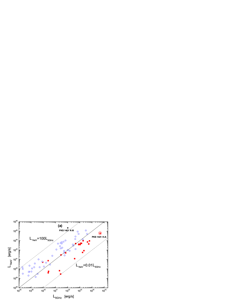
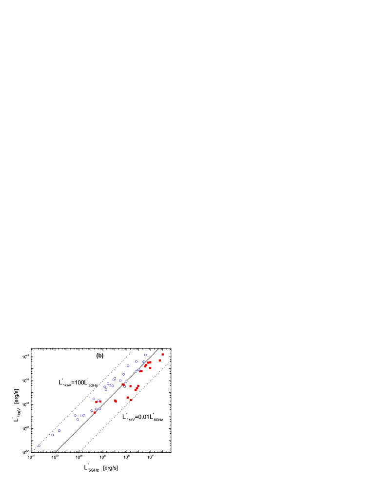
Figure 3: Luminosity at 1 keV as a function of that at 5 GHz for the knots and hot spots without (Panel a) and with (Panel b) corrected by the beaming factors. The symbols are the same as in Fig. 2.

Figure 3(a) shows the correlations between the observed luminosities at 5 GHz and 1 keV ($L_{\rm 5GHz}$ and $L_{\rm 1keV}$) for the hot spots and the knots. It is found that $L_{\rm 1keV}$ is tightly correlated with $L_{\rm 5GHz}$. We measure the correlations with the Spearman correlation analysis, which yields $\log L_{\rm 1keV}=(6.2\pm 4.7)+(0.84\pm 0.11)\log L_{\rm 5GHz}$ with a correlation coefficient $r=0.86$ and a chance probability $p<10^{-4}$ for the hot spots and $\log L_{\rm 1keV}=(6.9\pm 2.2)+(0.85\pm 0.05)\log L_{\rm 5GHz}$ with $r=0.92$ and $p<10^{-4}$ for the knots. The slopes of the two correlations are the same in the error scopes, but averagely speaking, the X-ray luminosity of the knots is larger than that of the hot spots with $\sim 0.7$ order of magnitude, indicating systematical difference between the two kinds of sources. As seen in §3.3, this correlation is much tighter by correcting with the Doppler boosting effect (see Figure 3(b) and details in §3.3). The knots and the hot spots in the $L_{\rm 5GHz}$-$L_{\rm 1keV}$ plane are roughly separated with a division line of $L_{\rm 1keV}=L_{\rm 5GHz}$. Therefore, the ratio of $R_{L}\equiv L_{\rm 5GHz}/L_{\rm 1keV}$ is a characteristic to distinguish the hot spots and the knots. This ratio should be an intrinsic parameter independent of the Doppler boosting effect and the cosmological effect. It may reflect the properties of the radiation regions.

3 modeling the Observed SEDs

The tight $L_{\rm 5GHz}$-$L_{\rm 1keV}$ correlation indicates that the radiations in the two energy bands may be produced by the same electron population. For few cases, such as hot spots N1 and N2 in 3C 33 and knots in M87 (Kraft et al. 2007; Liu & Shen 2007), their X-ray spectra are soft with $\alpha_{X}>1$, and smoothly connect to the spectrum in the radio and optical band. The X-rays of these sources may be the high energy tail of the synchrotron radiation by the same electron population for the radio and optical emission. The synchrotron radiation model is preferred to fit the X-rays of these sources.

Some well-sampled SEDs in Figure 1 roughly show two bumps similar to that observed in blazars. The two-bump feature is generally interpreted with the synchrotron radiation and IC scattering by the relativistic electrons. Therefore, we fit these SEDs with single-zone synchrotron + IC scatting models. The IC seed photons may be originated from the synchrotron radiation itself (SSC) or from the CMB. The photon field energy density of synchrotron radiation in the co-moving frame is given by $U^{{}^{\prime}}_{\rm syn}=L_{\rm syn}/(4\pi R^{2}c\delta^{4})\approx 2.65\times 10^{-12}L_{\rm syn,40}R^{-2}_{20}\delta^{-4}$ erg cm^-3, where $Q_{n}=Q/10^{n}$ in cgs units, $\delta$ the beaming factor, $R$ the radius of the radiation region, and $c$ the speed of light. The energy density of the CMB is $U_{\rm CMB}\approx 4\times 10^{-13}(1+z)^{4}\Gamma^{2}$ erg cm^-3, which dramatically increases with the redshift $z$ of the sources and the bulk Lorentz factor $\Gamma$ (taking $\Gamma\simeq\delta$) of the radiation site. Without considering the Doppler boosting effect, the IC component should be dominated by the SSC process, but it may be dominated by the IC/CMB, if the source is relativistic motion. We take the two scenarios into account.

In our models, the radiation region is assumed to be a homogeneous sphere with radius $R$. The radius is derived from the angular radius $\theta$ (see table 2), which is obtained from the optical or the X-ray observations. Considering the beaming effect, R and volume V of the emitting region are needed to take a relativistic transformation. We simply assume that the emitting region still is a sphere with $V^{{}^{\prime}}=V/\delta$ and derive the radius of emitting region in co-moving frame by $\emph{R}^{{}^{\prime}}=(3V^{{}^{\prime}}/4\pi)^{1/3}$. The electron distribution as a function of electron energy ($\gamma$) is taken as a single power-law or a broken power law,

$$N(\gamma)=N_{0}\left\{\begin{array}[]{ll}\gamma^{-p_{1}}&\mbox{ $\gamma\leq\gamma_{b}$},\\ \gamma_{b}^{p_{2}-p_{1}}\gamma^{-p_{2}}&\mbox{ $\gamma>\gamma_{b}$,}\end{array}\right.$$ (1)

where $p_{1,2}=2\alpha_{1,2}+1$ are the energy indices of electrons below and above the break energy $\gamma_{b}$, and $\alpha_{1,2}$ are the observed spectral indices.

In our calculations, the Klein-Nishina effect for the radiation in the GeV-TeV band is considered, but the absorption in the GeV-TeV band by the infrared background light and by CMB photon during the gamma-ray photons propagating to the Earth (Stecker et al. 2006) is not taken into account.

3.1 Equipartition Magnetic Field and the Synchrotron Radiation model

As mentioned in §1, the equipartition condition, which assumes that the magnetic field energy density $U_{B}$ is equal to the electron energy density $U_{e}$, is usually adopted in discussion of the X-ray origin. We first derive the magnetic field strength $B_{\rm eq}^{\delta=1}$ (see Appendix A) under this condition for the hot spots and knots in our sample without considering the beaming effect ($\delta=1$). The calculation of $B_{\rm eq}^{\delta=1}$ depends on $\gamma_{\min}$ (see Eqs. A5 and A10). The $\gamma_{\min}$ is quite uncertain (e.g., Harris & Krawczynski 2006). The $\gamma_{\min}$ values of 12 hot spots and all the knots in our sample are constrained with the observed SEDs via a method reported by Tavecchio et al. (2000). The average of $\gamma_{\min}$ for the 12 hot spots is $\sim 200$. For those hot spots that their $\gamma_{\min}$ lost constraints from the observed SEDs, we take $\gamma_{\min}=200$ in our calculation.

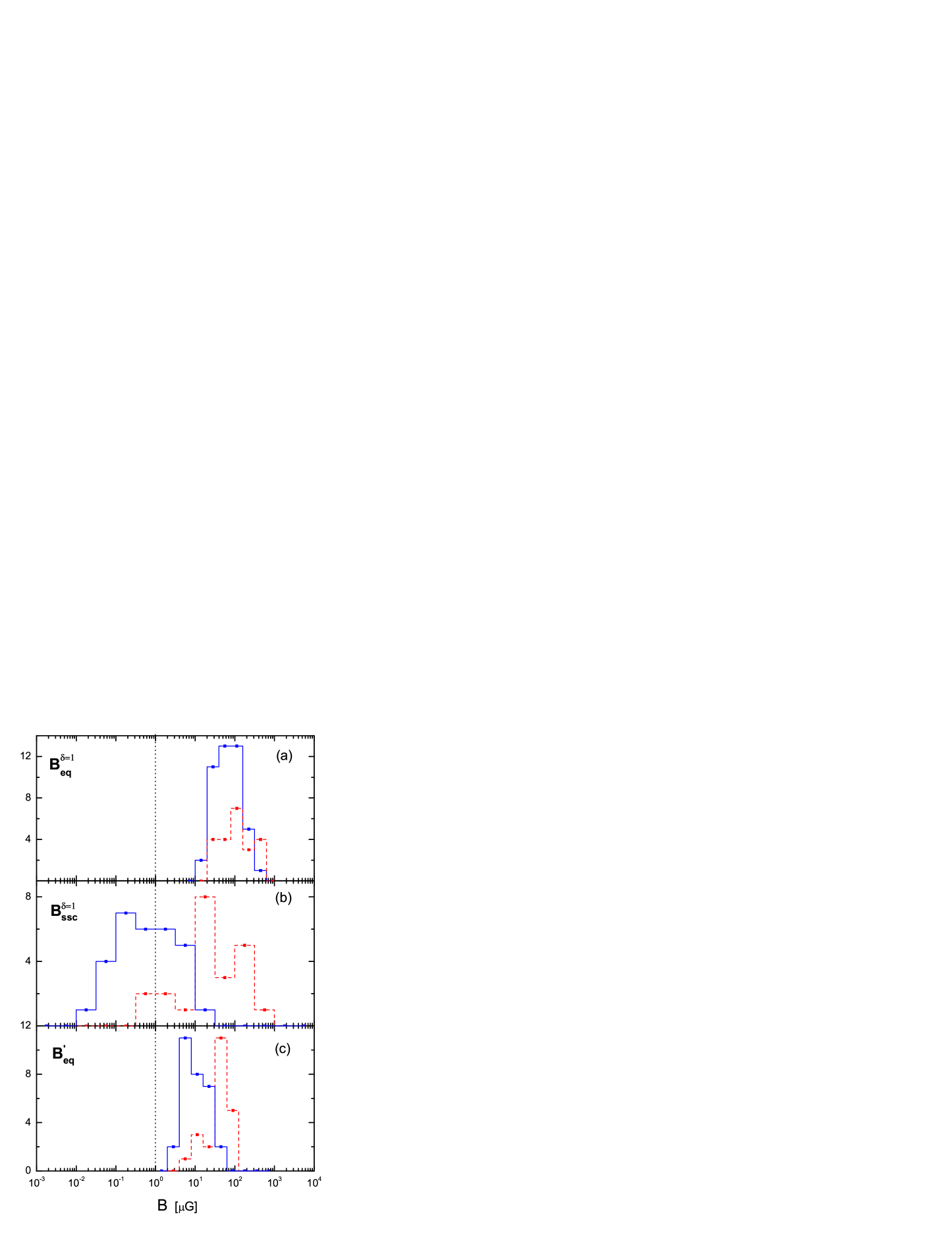
Figure 4: Distributions of the magnetic field strength for the knots and hot spots in cases of (a) assuming equipartition condition and $\delta=1$, (b) derived from the SSC model by assuming $\delta=1$, and (c) considering the beaming effect. The vertical dotted line is the magnetic field strength for the interstellar medium, i.e. $B=1\mu$G. The symbol styles are the same as in Fig. 2.

We fit the observed SEDs in the radio-optical band with the synchrotron radiation model to derive $B_{\rm eq}^{\delta=1}$. Our results are reported in Table 2. They are roughly consistent with the results derived from the formulae given by Brunetti et al. (1997). The distributions of $B_{\rm eq}^{\delta=1}$ for both the hot spots and knots are shown in Figure 4(a). They range in $10\sim 700$ $\mu$G. No systematical difference of $B_{\rm eq}^{\delta=1}$ is found between the two kinds of sources.

The observed X-ray spectra of the knots in 4C 73.18 (K-A), PKS 0521 (K), M87 (K-A, B, C1, D, E, F), 3C 31 (K), 3C 66B (K-B), and 3C 120 (K-K7) smoothly connect to the spectra in the radio and optical band. They are well fit with the synchrotron radiation model (the thin solid line in Figure 1), indicating that the X-rays of these sources are the high energy tail of the synchrotron radiation by the same electron population for the radio and optical emission. We do not take these sources into account in our following analysis.

3.2 Representing the X-rays with SSC model for the Sources at Rest

The observed X-ray spectral indices and SEDs shown in Table 2 and Figure 1 indicate that the X-rays of most hot spots and knots should be contributed by IC scattering. We model the SEDs with the synchrotron + IC model assuming that the sources are at rest. In this scenario, the SSC process should dominate the IC process, as mentioned above. Although the contribution of IC/CMB to the X-ray emission is not negligible for some sources at high redshift, we only consider the SSC component in this section.

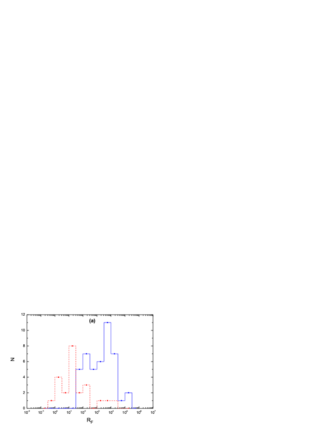
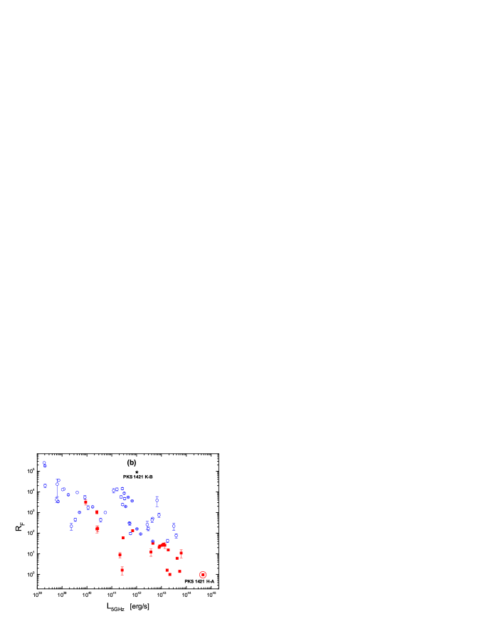
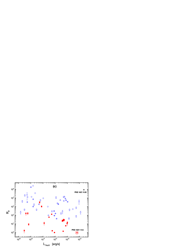
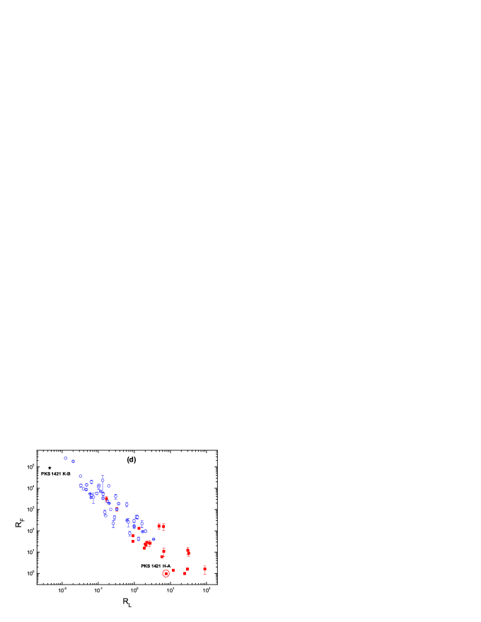
Figure 5: Panel a—Distributions of the ratio ($R_{F}$) of the observed flux density at 1 keV to that of expected from the SSC model with $B=B^{\delta=1}_{\rm eq}$. Panels b,c,d—$R_{F}$ as a function of the luminosities at 5 GHz and 1 keV bands and the radio ($R_{L}$) of the luminosities in the two energy bands for the knots and hot spots. The symbol styles are the same as in Fig. 2.

We first calculate the X-ray flux density at 1 keV ($F_{\rm 1keV}^{\rm eq}$) with the synchrotron + SSC model under the equipartition assumption, i.e., $B=B_{\rm eq}^{\delta=1}$. Our results are reported in Table 2. We measure the consistency between $F_{\rm 1keV}^{\rm eq}$ and $F_{\rm 1keV}^{\rm obs}$ with ratio $R_{F}\equiv F_{\rm 1keV}^{\rm obs}/F_{\rm 1keV}^{\rm eq}$, where $F_{\rm 1keV}^{\rm obs}$ is the observed flux density at 1 keV. It is found that $R_{F}$ is much larger than 1 for almost all the hot spots and knots in our sample, indicating that the observed X-ray flux density is much larger than the model prediction. The distributions of $R_{F}$, and $R_{F}$ as a function of $L_{\rm 5GHz}$, $L_{\rm 1keV}$, and $R_{L}$ for the hot spots and knots are shown in Figure 5. A tentative correlation presented in the $R_{F}-L_{\rm 5GHz}$ plane shows that the brighter sources in the radio band tend to be more consistent with the equipartition condition (see Figure 5(b)). However, no similar feature is seen for the X-ray bright sources (see Figure 5(c)). It is interesting that $R_{F}$ is anti-correlated with $R_{L}$, and both the hot spots and knots shape a well sequence (see Figure 5(d)). The hot spots are at the lower end of the sequence and they tend to be closer to the equipartition condition than the knots.

As shown above, the derived X-ray flux densities from the SSC model under the equipartition condition significantly deviate the observations, especially for the knots. In order to model the observed SEDs with the synchrotron + SSC model, we have to get rid of this assumption. Keeping the model parameters the same as that used above, we fit the SEDs with this model and derive the magnetic field strengths ($B^{\delta=1}_{\rm ssc}$). The fits are shown in Figure 1 (the thick solid line). Although the SSC model can represent the observed flux at 1 keV for the knots in 4C 73.18 (K-A), PKS 0521, M87 (K-A, B, C1, D, E, F), 3C 31, 3C 66B (K-B), 3C 120 (K-K7), 3C 273 (K-C1, C2, D1, D2H3), the bow ties defined by the errors of the X-ray spectral indices clearly rule out this model for these knots. As discussed in Section 3.1, the X-rays of these knots are well fitted by the synchrotron radiation model except knots in 3C 273. We do not include these knots in our following statistics.

The derived $B^{\delta=1}_{\rm ssc}$ are listed in Table 2, and their distributions are shown in Figure 4(b). It is found that the $B^{\delta=1}_{\rm ssc}$ of the knots are much smaller than the hot spots, with medians of $1\mu$G and $\sim 30$ $\mu$G for the knots and hot spots, respectively. Comparing $B^{\delta=1}_{\rm ssc}$ with $B^{\delta=1}_{\rm eq}$, it is found that they are roughly consistent for the hot spots, indicating that the X-rays of the hot spots can be roughly fitted with the SSC model under the equipartition condition. However, the $B^{\delta=1}_{\rm ssc}$ of the knots are much smaller than $B^{\delta=1}_{\rm eq}$, even unreasonably smaller than the magnetic field strength of the interstellar medium for some knots. Therefore, the X-rays of these knots may not be dominated by the SSC component.

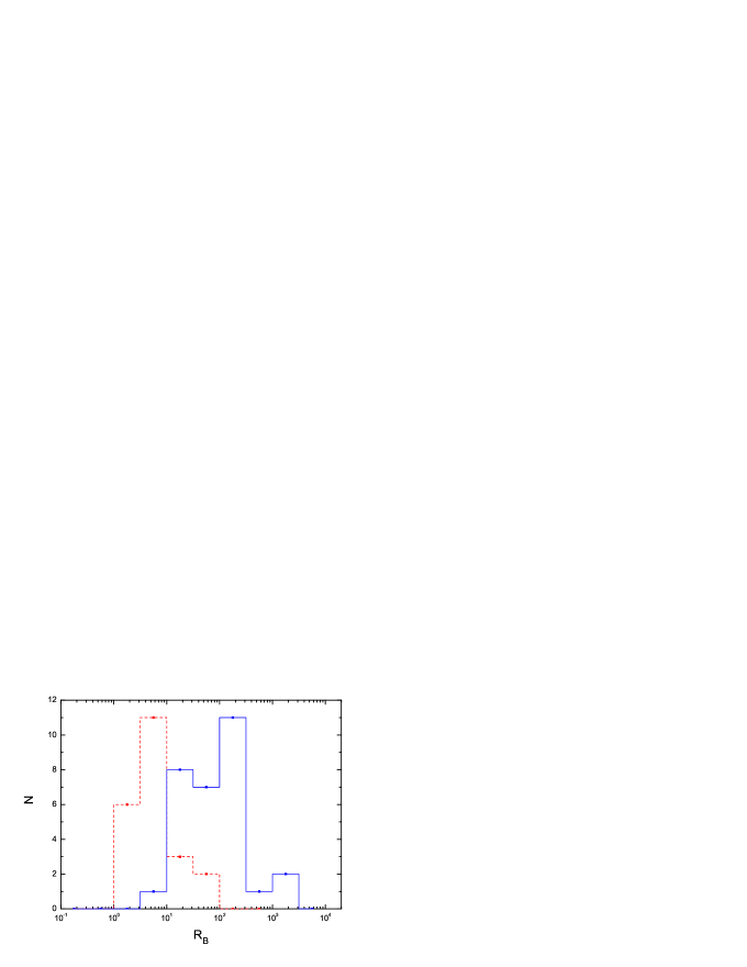
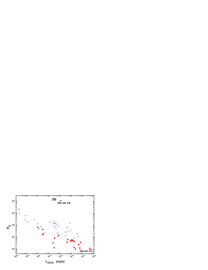
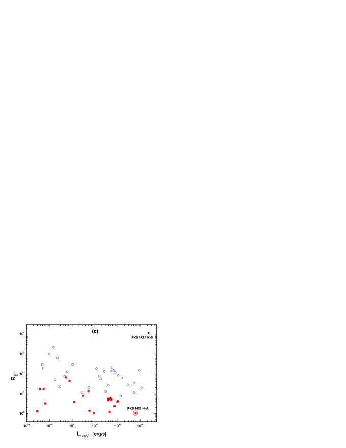
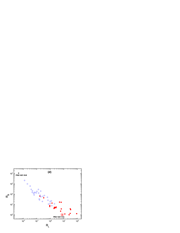
Figure 6: Panel a—Distributions of the ratio ($R_{B}$) of the equipartition magnetic field strength to $B_{\rm ssc}^{\delta=1}$, the magnetic field strength derived from the SSC model by assuming $\delta=1$. Panels b,c,d—$R_{B}$ as a function of the luminosities at 5 GHz and 1 keV bands and the radio ($R_{L}$) of the luminosities in the two energy bands for the knots and hot spots. The symbol styles are the same as in Fig. 2.

To investigate the deviation of $B^{\delta=1}_{\rm ssc}$ to $B^{\delta=1}_{\rm eq}$ for individual source, we define ratio $R_{B}\equiv B^{\delta=1}_{\rm eq}/B^{\delta=1}_{\rm ssc}$, which is physically the same as $R_{F}$. Similar to $R_{F}$, $R_{B}$ is much larger than 1 for almost all the sources, especially for the knots. The distributions of $R_{B}$ and $R_{B}$ as a function of $L_{\rm 5GHz}$, $L_{\rm 1keV}$, and $R_{L}$ are shown in Figure 6. We find the same features as shown in Figure 5.

3.3 Modeling the X-Rays by Considering Relativistic Bulk Motion

It is generally believed that the knots should have relativistic motion. The hot spots may also be relativistic (Dennett-Thorpe et al. 1997; Tavecchio et al. 2005; Harris & Krawczynski 2006). In this section, we fit the SEDs with the synchrotron + IC model by considering the beaming effect under the equipartition condition. In this scenario, the IC/CMB process should dominate the IC component. Although the contribution of SSC is negligible comparing with IC/CMB in this case, we still take SSC process into account in our calculation.

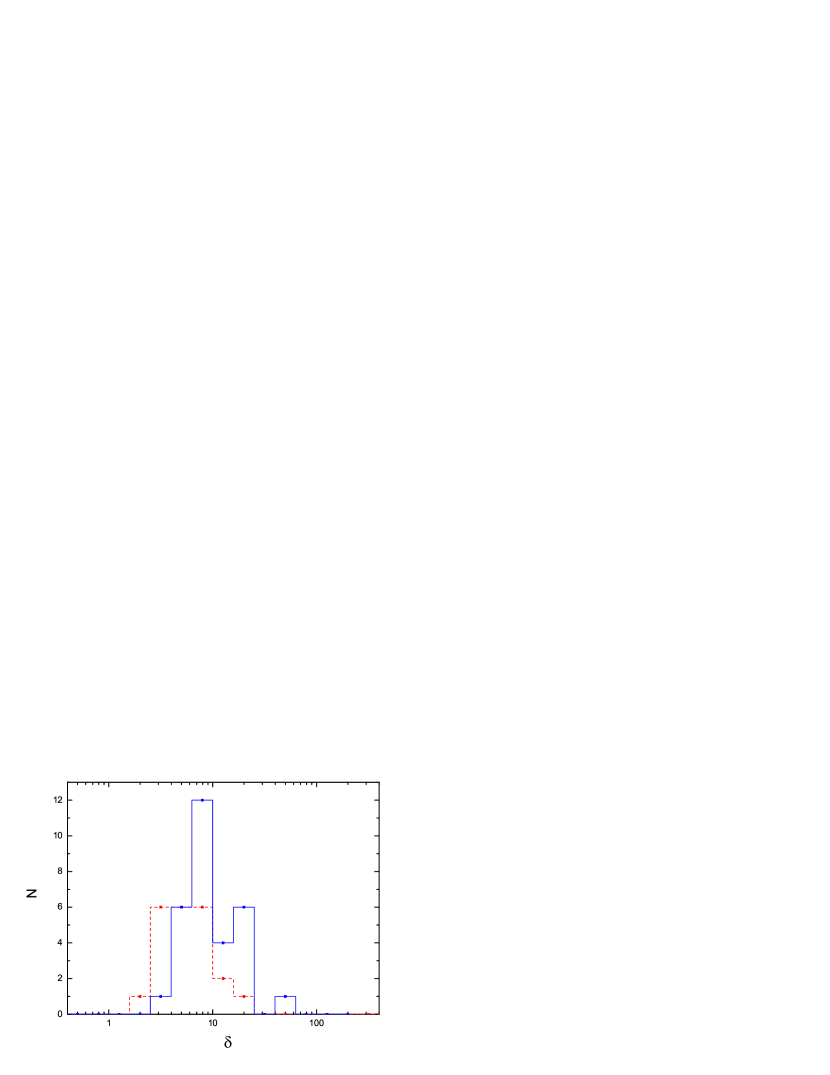
Figure 7: Distributions of the beaming factors for the knots and hot spots. The symbols are the same as in Fig. 2.

Our fits are shown in Figure 1 (the dashed line). The distributions of $\delta$ for the knots and hot spots are shown in Figure 7. It is found that, averagely, $\delta\sim 10$ for most of the knots and $\delta\sim 5$ for most of the hot spots. Some sources in our sample are included in Kataoka & Stawarz (2005). We compare our results of $\delta$ for these sources with that reported by Kataoka & Stawarz (2005) ($\delta^{\rm KS05}$) in Figure 8. They are roughly consistent.

The $B_{\rm eq}^{{}^{\prime}}$ distributions with comparison to $B_{\rm eq}^{\delta=1}$ and $B_{\rm SSC}^{\delta=1}$ are shown in Figure 4(c). The $B_{\rm eq}^{{}^{\prime}}$ distributions are more consistent with $B_{\rm eq}^{\delta=1}$ than $B_{\rm SSC}^{\delta=1}$. Both $B_{\rm eq}^{{}^{\prime}}$ and $B_{\rm eq}^{\delta=1}$ distributions approximately span an order of magnitude, much narrower than that of $B_{\rm SSC}^{\delta=1}$, especially for the knots. All $B_{\rm eq}^{{}^{\prime}}$ are larger than the magnetic filed strength of the interstellar medium, implying that the magnetic filed of the interstellar medium would be amplified in the knots and hot spots by the turbulence of the relativistic shocks. The $B_{\rm eq}^{{}^{\prime}}$ of the knots are smaller than that of the hot spots, with typical values of 10 $\mu$G and 40 $\mu$G for the knots and the hot spots, respectively, favoring the idea of different origins of the shocks (internal vs. external) for the two kinds of sources (e.g., Harris & Krawczynski 2006).

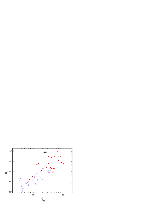
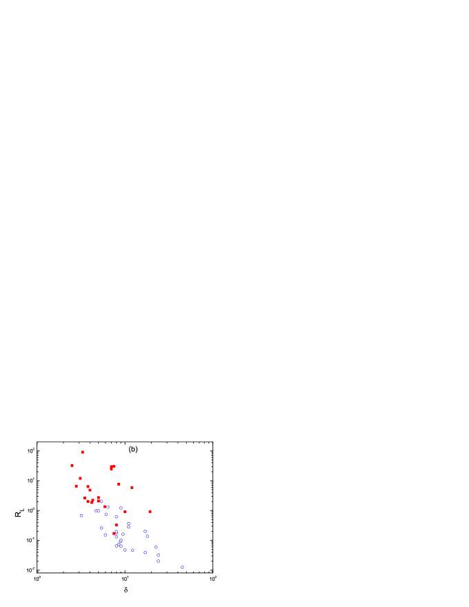
Figure 9: Panel b—Correlations of $R_{L}$ with $B_{\rm eq}^{{}^{\prime}}$ (panel a) and $\delta$ (panel b) for the knots and hot spots. The symbol styles are the same as in Fig. 2.

As our discussed in §2, $R_{L}$ is an intrinsic characteristic for the sources. It may be a representative of the co-moving magnetic field and the Doppler boosting effect of the sources. We show $R_{L}$ as a function of $B_{\rm eq}^{{}^{\prime}}$ and $\delta$ in Figure 9. It is found that $R_{L}$ is correlated with $B_{\rm eq}^{{}^{\prime}}$ for the knots, with a linear coefficient of $r=0.77$ and chance probability $p<10^{-4}$. We obtain $\log R_{L}=(-2.23\pm 0.24)+(1.45\pm 0.23)\log B_{\rm eq}^{{}^{\prime}}$. No significant correlation between $R_{L}$ and $B_{\rm eq}^{{}^{\prime}}$ is found for the hot spots. However, both the knots and hot spots form a sequence in the $R_{L}-B_{\rm eq}^{{}^{\prime}}$ plane, with a best linear fit $\log R_{L}=(-2.55\pm 0.23)+(1.92\pm 0.17)\log B_{\rm eq}^{{}^{\prime}}$. The hot spots locate at the higher end of the sequence. Similar feature is also observed in the $R_{L}-\delta$ plane, as shown in Figure 9(b). These results imply that $R_{L}$ would be determined by both $B_{\rm eq}^{{}^{\prime}}$ and $\delta$. The strong anti-correlation of $R_{F}-R_{L}$ (or $R_{B}-R_{L}$) shown in Figure 5 (or Figure 6) may be due to neglect of the beaming effect. This effect plays important role on the observed flux since the observed flux is proportional to $\delta^{4}$. Correcting by the Doppler boosting effect, we show the $L_{\rm 5GHz}^{{}^{\prime}}-L_{\rm 1keV}^{{}^{\prime}}$ relations in Figure 3(b). The relations are tighter than the observed ones, with a linear coefficient of $r=0.98$ and $r=0.90$ for the knots and hot spots, respectively.

4 Conclusions and Discussion

We have present extensive analysis and SED fits for 22 hot spots and 45 knots in 35 AGN jets. We find that $L_{\rm 5GHz}$ and $L_{\rm 1keV}$ are tightly correlated. The two kinds of sources can be roughly separated with a division of $L_{\rm 1keV}\sim L_{\rm 5GHz}$. Our SED fits show that the mechanisms of the X-rays are diverse. While the X-ray emission of a small fraction of the sources is a simple extrapolation of the synchrotron radiation for the radio-to-optical emission, the IC component may dominate the observed X-rays for most of the sources. Without considering the relativistic bulk motion, the SSC model can explain the X-rays for some hot spots with $B_{\rm ssc}^{\delta=1}$ being consistent with the equipartition magnetic field $B_{\rm eq}^{\delta=1}$ in one order of magnitude, but an unreasonably low magnetic field strength is required in modeling the X-rays for all knots with this model. Considering relativistic bulk motion for the sources, the IC/CMB dominated model well explains the X-ray emission for most sources under the equipartition condition. Although the derived $B_{\rm eq}^{{}^{\prime}}$ and $\delta$ for some hot spots are comparable to that of the knots, the $B_{\rm eq}^{{}^{\prime}}$ value for the knots tends to be smaller than that of the hot spots and the $\delta$ tends to be larger, favoring the idea that the hot spots are jet termination and knots are a part of a well-collimated jet. Corrected by the beaming effect, the $L^{{}^{\prime}}_{\rm 5GHz}-L^{{}^{\prime}}_{\rm 1keV}$ relations for the two kinds of sources are even tighter than the observed ones, indicating that the correlations are intrinsic. The ratio $R_{L}$ is correlated with $B_{eq}^{{}^{\prime}}$ and $\delta$. These facts suggest that, under the equipartition condition, the differences on the X-ray observations for the knots and hot spots would be mainly due to the differences of the Doppler boosting effect and the co-moving magnetic field, although some hot spots have similar feature to the knots.

The $R_{L}$ may be an indicator of $B_{eq}^{{}^{\prime}}$ and $\delta$. It is an intrinsic parameter independent of the Doppler boosting and the cosmological effects. Our results show that the X-rays of a hot spot with larger $R_{L}$ are better to be fitted with the SSC model under equipartition condition without considering the beaming effect. This is consistent with that reported by Hardcastle et al. (2004), who found that the X-rays of the radio-bright hot spots can be explained with the SSC model under equipartition condition. The strong anti-correlation between $R_{B}$ (or $R_{F}$) and $R_{L}$ may also offer a tool to discriminate the two kinds of sources. We find in the Figures 3, 5 and 6 that the hot spot H-A and the knot K-B in PKS B1421-490 are significant outliers. They were reported as knots by Gelbord et al. (2005). The knot K-B is very peculiar for its extreme optical output, with a ratio of knot/core optical flux $\sim 300$. Gelbord et al. (2005) suspected that it is a core between components A and C. We find that K-B looks is a significant outlier in the figures and K-A resembles a hot spot. Most recently, Godfrey et al. (2009) confirmed that the K-B is a core and the K-A is a hot spot with VLBI observations.

The $B_{\rm eq}^{{}^{\prime}}$ value for the knots tends to be smaller than that of the hot spots and the $\delta$ tends to be larger, favoring the idea that the hot spots are jet termination and knots are a part of a well-collimated jet. However, the $B_{\rm eq}^{{}^{\prime}}$ and $\delta$ for some hot spots are comparable to that of the knots, making uncertainty on identifying a component as a knot or a hot spot. For example, the north-east double hot spots in 3C 351, which locate at the outer boundary of a lobe, have relativistic motion feature, hence may be identified as knots of the jet (Harris & Krawczynski 2006).

The synchrotron radiation in the optical band indicates that there are relativistic electrons existed in these extended regions (Roser & Meisenheimer 1987; L$\ddot{a}$hteenmäki & Valtaoja 1999). Moreover, the X-ray emission of some sources may be also synchrotron radiation as mentioned in §3.1. Assuming a magnetic field strength $B\sim 10^{-5}$ G, one can estimate the energy of relativistic electrons is $\gamma\sim 10^{6}$, which contribute to the optical emission by synchrotron process. These electrons may interact with the synchrotron photons and external field photons to produce very high energy $\gamma$-ray photons by IC scattering. As shown in Figure 1, both the SSC and IC/CMB models predict a prominent GeV-TeV component in the SEDs of some sources. We check if the predicted GeV-TeV emission can be detectable with H.E.S.S. and Fermi/LAT, and also show the sensitivity curves of H.E.S.S. and Fermi/LAT in Figure 1 for these sources. The detections of these high energy emission would place much stronger constraints on the radiation mechanisms and on the physical parameters of these sources. The origin of the high energy TeV gamma-ray emission is also a debating issue, and detections of these high energy emission would drastically improved our view of the universe (see Cui 2009 for a review).

Note that our one-single zone lepton models cannot explain the observed SEDs for the four knots in 3C 273 (K-C1, K-C2, K-D1, and K-D2H3). Jester et al. (2006) had reported that the X-ray spectra rule out the single-zone model of X-ray emission for some jet knots in 3C 273. It is possible that these sources may have a complex structure as the western hot spot in Pictor A (Zhang et al. 2009).

Table 1: List of 35 AGNs with jet knots and hot spots included in our sample

Name	z	$D_{L}$ (Mpc)	Class	Reference
3C 15	0.073	329.9	RG (FR I/II)	1
3C 31	0.0169	73.3	RG (FR I)	2
3C 33	0.0597	267.3	RG (FR II)	3
3C 228	0.5524	3194	RG	4
3C 245	1.029	6845.4	Q	5
3C 263	0.6563	3937	LDQ	6
3C 275.1	0.557	3226.2	LDQ	4
3C 280	0.996	6575	RG (FR II)	7
3C 351	0.371	1988	LDQ	6
3C 390.3	0.0561	250.5	RG (FR II)	8
3C 295	0.461	2570.6	RG (FR II)	9
3C 303	0.141	666.6	RG (FR II)	10
3C 66B	0.0215	93.6	RG (FRI)	2
3C 120	0.033	144.9	Sy I	12
3C 273	0.1583	756.5	CDQ	13
3C 454.3	0.86	5485.1	CDQ	14
3C 207	0.684	4141	LDQ	5
3C 345	0.594	3487.4	CDQ	5
3C 346	0.161	770.7	RG (FR I)	15
3C 371	0.051	226.9	BL	16
3C 403	0.059	264	RG (FR II)	17
M87	0.0043	18.5	RG (FR I)	20
Cygnus A	0.0562	251	RG (FR II)	11
Pictor A	0.035	153.9	RG (FR II)	21
PKS 0405-123	0.574	3345.6	Q	5
PKS 0521-365	0.0554	247.3	BL	22
PKS 0637-752	0.653	3913.1	CDQ	2
PKS 1136-135	0.554	3205.2	LDQ	18
PKS 1229-021	1.045	6977.3	CDQ	14
PKS 1421-490	0.663	3986.3	Q	19
PKS 2201+044 ((4C 04.77))	0.027	118	BL	16
PKS 1928+738 (4C +73.18)	0.302	1564.7	CDQ	5
PKS 1354+195 (4C +19.44)	0.72	4409.1	CDQ	5
PKS 1150+497 (4C +49.22)	0.334	1758.4	CDQ	5
PKS 0836+299 (4C +29.30)	0.064	287.4	RG (FR I)	5

References. — (1) Kataoka et al. 2003a; (2) Kataoka & Stawarz 2005; (3) Kraft et al. 2007; (4) Hardcastle et al. 2004; (5) Sambruna et al. 2004; (6) Hardcastle et al. 2002; (7) Donahue et al. 2003; (8) Harris et al. 1998; (9) Harris et al. 2000; (10) Meisenheimer et al. 1997; Kataoka et al. 2003b; (11) Stawarz et al. 2007; (12) Harris et al. 2004; (13) Jester et al. 2007; (14) Tavecchio et al. 2007; (15) Worrall & Birkinshaw 2005; (16) Sambruna et al. 2007; (17) Kraft et al. 2005; (18) Sambruna et al. 2006; (19) Gelbord et al. 2005; (20) Liu & Shen 2007; Perlman et al. 2001; (21) Wilson et al. 2001; (22) Falomo et al. (2009).

Table 2: Observations and SED fit results for the hot spots and knots in our sample

		Observations					$\delta=1$, SSC				$\delta>1$, IC/CMB			Preferred model
Source	Comp	$\alpha_{r}$	$\alpha_{X}$	$F_{\rm 1keV}^{\rm obs}$	$\theta$	$\gamma_{\min}$	$B^{\delta=1}_{\rm eq}$	$F_{\rm 1keV}^{\rm eq}$	$B^{\delta=1}_{\rm ssc}$		$\delta$	$B^{{}^{\prime}}_{\rm eq}$		Model	$\alpha_{X}^{\rm mod}$	$p_{1}$	$p_{2}$
				(nJy)	(arcsec)		($\mu$G)	(nJy)	($\mu$G)			($\mu$G)
(1)	(2)	(3)	(4)	(5)	(6)	(7)	(8)	(9)	(10)		(11)	(12)		(13)	(14)	(15)	(16)
3C 33	H-S1	0.75	0.8$\pm$0.6	0.14$\pm$0.06	0.5	200	158	0.086	120		3.3	66.1		SSC	0.63	2.4	4.4
	H-S2	0.98	0.8$\pm$0.6	0.32$\pm$0.09	1.5	200	64.6	0.036	20		2.5	32.9		SSC	0.71	2.56	3.98
	H-N1	0.88	1.2$\pm$0.8	0.27$\pm$0.08	1.25	200	36.4	0.0016	2.1		4	13.2		SYN	1.85	2.4	3.6
	H-N2	0.9	1.2$\pm$0.8	0.19$\pm$0.07	1.25	200	38.7	0.0012	2.3		3.8	14.6		SYN	1.41	2.38	3.8
3C 263	H-K	0.84	1.0$\pm$0.3	1.0$\pm$0.1	0.39	300	144	0.71	118		3.1	70		SSC	0.8	2.62	4.04
Cygnus A	H-A	0.5	0.77$\pm$0.13	31.2$\pm$4.3	1	200	214	19.4	155		7	52.4		SSC	0.8	1.84	3.86
	H-D	0.38	0.8$\pm$0.11	47.9$\pm$5.9	1	100	164	47.8	160		7	40.7		SSC	0.77	1.5	3.24
	H-B	0.59	0.7$\pm$0.35	6.8$\pm$2.6	1	200	330	0.55	85		7.5	78.9		SSC	0.77	2.02	3.96
3C 351	H-L	0.93	0.85$\pm$0.1	3.4$\pm$0.4	0.8	300	72.4	0.13	12.5		5	28		SSC	0.78	2.36	3.3
	H-J	0.76	0.5$\pm$0.1	4.3$\pm$0.3	0.16	200	186	0.13	29		10	33.1		IC/CMB	0.34	2.44	3.1
3C 303	H-W	0.84	0.4$\pm$0.2	4	1	200	68.9	0.03	5		5.9	18.6		IC/CMB	0.5	2.64	3.7
3C 295	H-NW	0.94	0.9$\pm$0.5	3.8	0.1	500	460	0.63	200		12	102.9		SSC	0.94	1.9	4.4
3C 390.3	H-B	0.71	0.9$\pm$0.15	4.2$\pm$0.87	1	200	38.1	0.004	0.85		8	9.45		IC/CMB	0.78	2.56	3.1
3C 275.1	H-N	$\cdots$	$\cdots$	1.78	0.6	100	119	0.061	22		4.3	40.3		SSC	0.84	2.79	$\cdots$
3C 228	H-S	$\cdots$	$\cdots$	1.3	0.27	200	131	0.063	28		5	40		SSC	0.87	2.62	3.1
3C 245	H-D	$\cdots$	$\cdots$	0.7$\pm$0.3	0.8	600	67.7	0.064	18		2.8	32		SSC	0.66	1.96	3.92
3C 280	H-W	0.8	1.3$\pm$1.0	0.79	0.3	200	147	0.052	35		4.2	51.2		SYN	1.22	2.6	3.3
	H-E	0.8	1.2	0.34	0.3	200	124	0.014	23		3.8	46.5		SYN	1.13	2.6	3.1
PKS 0405	H-N	$\cdots$	$\cdots$	1.6$\pm$0.5	0.7	400	81.8	0.061	16.5		3.5	37.2		SSC	0.91	2.8	3.22
PKS 0836	H-B	$\cdots$	$\cdots$	2.2$\pm$0.6	0.9	100	33.1	6.9E-4	0.5		7.5	7.45		SYN	1.04	2.68	3.06
Pictor A	H-W	0.74	1.07$\pm$0.11	45	0.3	110	392	0.76	48		19.3	45.3		SYN	1.32	2.38	3.66
PKS 1421	H-A	0.67	0.31$\pm$0.32	13.3$\pm$1.6	0.24	200	404	13.7	400		8.5	86.2		SSC	0.6	1.9	4.06
M87	K-D	$\cdots$	1.43$\pm$0.09	51.5$\pm$4.2	0.4	150	296	0.015	2.8		$\cdots$	$\cdots$		SYN	1.34	2.36	3.68
	K-A	$\cdots$	1.61$\pm$0.07	156$\pm$8.8	0.9	150	266	0.15	5		$\cdots$	$\cdots$		SYN	1.55	2.28	4.1
	K-E	$\cdots$	1.48$\pm$0.12	32.2$\pm$6.5	0.9	150	101	0.0016	0.38		$\cdots$	$\cdots$		SYN	1.38	2.42	3.76
	K-F	$\cdots$	1.64$\pm$0.15	20.1$\pm$5.2	1.2	150	118	0.0049	0.9		$\cdots$	$\cdots$		SYN	1.53	2.3	4.06
	K-B	$\cdots$	1.59$\pm$0.12	30.3$\pm$5.5	1.3	150	184	0.066	5.5		$\cdots$	$\cdots$		SYN	1.77	2.32	4.54
	K-C1	$\cdots$	1.33$\pm$0.06	14.6$\pm$5.2	0.5	100	380	0.067	20		$\cdots$	$\cdots$		SYN	1.7	2.36	4.4
PKS 1136	K-A	0.67	1.1$\pm$0.6	1.7$\pm$0.2	0.85	50	25.7	3.6E-4	0.18		8	5.68		IC/CMB	0.66	2.32	$\cdots$
	K-B	0.81	1.1$\pm$0.3	3.5$\pm$0.2	0.6	100	57.6	9.5E-4	0.67		9	11.4		IC/CMB	0.8	2.61	$\cdots$
	K-$\alpha$	0.75	0.9$\pm$0.4	1.9$\pm$0.2	0.75	60	34	1.3E-4	0.16		10	6.95		IC/CMB	0.71	2.42	$\cdots$
	K- D	0.71	0.5$\pm$0.5	1.0$\pm$0.2	0.6	100	94.7	0.0061	7.2		4.7	30		IC/CMB	0.9	2.8	$\cdots$
PKS 1150	K- B	0.72	0.7$\pm$0.2	7.6$\pm$0.5	0.76	100	41.8	8.8E-4	0.28		12.2	6.7		IC/CMB	0.72	2.46	4.6
	K-C	0.71	0.5$\pm$0.3	2.9$\pm$0.4	0.91	300	27	5.1E-4	0.2		8.9	6.18		IC/CMB	0.72	2.42	3.82
	K-D	0.68	0.7$\pm$0.5	1.3$\pm$0.3	0.91	50	28.4	1.1E-4	0.15		9	6.7		IC/CMB	0.69	2.38	$\cdots$
	K-E	0.67	0.7$\pm$0.3	1.7$\pm$0.2	0.71	800	27.6	7E-4	0.35		8	7.43		IC/CMB	0.68	2.36	3.4
	K-IJ	0.81	1.1$\pm$0.6	0.6$\pm$0.1	0.71	200	50.6	0.0021	2.5		5	17.2		IC/CMB	0.8	2.6	4.28
PKS 2201	K-A	0.71	1.1$\pm$0.4	5.6	0.5	100	37.2	1.5E-4	0.06		24	4.08		SYN	1.1	2.2	3.12
	K-$\beta$	0.59	0.9$\pm$0.5	3.8	0.3	50	67.4	1.5E-5	0.031		45	4.34		IC/CMB	0.53	2.15	5
3C 371	K-A	0.69	1.1$\pm$0.4	7	0.7	50	32.5	7.5E-4	0.11		17	4.14		SYN	1.09	2.34	3.12
PKS 1928	K-A	$\cdots$	1.66$\pm$0.74	6.9$\pm$1.1	0.8	100	36.4	5.2E-4	0.18		$\cdots$	$\cdots$		SYN	0.88	2.6	4.06
PKS 1354	K-A	$\cdots$	0.6$\pm$0.32	16.1$\pm$8.2	1.9	300	27.2	0.0041	0.18		8.5	5.92		IC/CMB	0.41	2.12	4
	K-B	$\cdots$	$\cdots$	0.7$\pm$0.3	1.4	300	23.5	0.0027	0.9		3.2	10.1		IC/CMB	0.5	2.32	3.4
PKS 1229	K-A	$\cdots$	$\cdots$	8.5$\pm$3.2	1	250	60.3	0.038	3		5.4	17.6		IC/CMB	0.63	2.4	3.6
PKS 0637	K	0.8	0.9$\pm$0.1	6.2	0.4	100	108	0.012	3.8		9.5	20.6		IC/CMB	0.8	2.6	$\cdots$
PKS 0521	K	0.89	1.3$\pm$0.3	14	0.4	100	118	0.014	2.5		$\cdots$	$\cdots$		SYN	1.25	2.4	3.5
3C 454.3	K-A	$\cdots$	$\cdots$	6$\pm$1.4	1	300	51.8	0.008	1.5		6	13.8		IC/CMB	0.3	2.6	5
	K-B	$\cdots$	$\cdots$	6$\pm$1.4	1	40	95.1	0.079	8.5		6.1	34.6		IC/CMB	0.72	2.44	5
3C 403	K-F1	$\cdots$	0.75$\pm$0.4	0.9$\pm$0.2	0.75	150	56.3	5.2E-4	1.1		8	13		IC/CMB	0.79	2.58	$\cdots$
	K-F6	$\cdots$	0.7$\pm$0.3	2.3$\pm$0.2	0.75	100	60.8	0.0012	0.8		11	10.6		IC/CMB	0.68	2.4	$\cdots$
3C 346	K-C	$\cdots$	1.0$\pm$0.3	1.6$\pm$0.2	0.9	100	72.3	0.017	6.1		5.4	20.9		IC/CMB	0.8	2.6	$\cdots$
3C 345	K-A	$\cdots$	0.66$\pm$0.86	3.8$\pm$0.7	0.6	50	131	0.089	17		6.4	36.6		IC/CMB	0.76	2.52	$\cdots$
3C 207	K-A	$\cdots$	0.1$\pm$0.3	3.0$\pm$0.7	0.5	100	62.7	0.007	1		11	11.2		IC/CMB	0.4	1.8	3.6
3C 66B	K-A	0.75	0.97$\pm$0.34	4.0$\pm$0.3	0.7	60	45.5	2.2E-5	0.045		24	4.47		SYN	1.16	2.46	3.4
	K-B	0.6	1.17$\pm$0.14	6.1$\pm$0.4	0.6	50	73.2	8.5E-4	0.33		$\cdots$	$\cdots$		SYN	1.27	2.22	3.54
3C 31	K-K	0.55	1.1$\pm$0.2	7.3	0.6	150	88.2	5.3E-4	0.2		$\cdots$	$\cdots$		SYN	0.98	2.72	3.4
3C 15	K-C	0.9	0.71$\pm$0.4	0.934$\pm$0.2	0.4	30	162	0.0021	7.2		9	31.6		IC/CMB	0.9	2.8	$\cdots$
3C 273	K-A	0.85	0.83$\pm$0.02	46.5$\pm$0.54	0.8	20	91.8	0.0085	0.77		22.5	12.2		IC/CMB	0.75	2.5	5
	K-C1	0.73	1.07$\pm$0.06	4.85$\pm$0.16	0.6	20	110	0.016	4.5		10.5	19.6		IC/CMB	0.74	2.48	4
	K-C2	0.75	0.96$\pm$0.05	6.25$\pm$0.18	0.7	20	118	0.039	6.8		9.5	22.7		IC/CMB	0.75	2.5	3.82
	K-B1	0.82	0.8$\pm$0.03	10.9$\pm$0.25	0.6	20	126	0.0056	2.2		17	21.8		IC/CMB	0.82	2.64	6
	K-D1	0.77	1.02$\pm$0.05	5.16$\pm$0.17	0.7	20	149	0.057	13		8.5	31		IC/CMB	0.79	2.58	4.74
	K-DH	0.85	1.04$\pm$0.04	7.82$\pm$0.2	1	20	174	0.19	25.5		6.8	41.9		IC/CMB	0.86	2.72	4.4
3C 120	K-K4	0.74	0.9$\pm$0.2	10$\pm$2	0.7	100	76.2	0.0018	0.58		18	9.24		IC/CMB	0.58	2.4	$\cdots$
	K-S2	0.67	0.2$\pm$0.6	0.882	1.6	100	17.1	6.9E-5	0.085		8	3.8		IC/CMB	0.62	2.24	$\cdots$
	K-S3	0.69	$\cdots$	0.8$\pm$0.6	1.6	100	16.1	3.4E-5	0.055		8	3.5		SYN	1.16	2.36	3.28
	K-K7	0.68	2.4$\pm$0.6	6.3$\pm$1.6	1.5	100	35.3	$\cdots$	$\cdots$		$\cdots$	$\cdots$		SYN	1.2	2.6	7

Note. — Columns: (3) Radio spectral index $\alpha_{r}$; (4) X-ray spectral index $\alpha_{x}$ at 1 keV; (5) The observed X-ray flux density at 1 keV; (6) Size of the emitting region in arcsec; (7) The minimum Lorentz factor of the electrons $\gamma_{min}$; (8) The equipartition magnetic field $B^{\delta=1}_{\rm eq}$; (9) The predicted flux density at 1 keV; (10) The fitting magnetic field $B^{\delta=1}_{\rm ssc}$ with SSC model; (11) The beaming factors $\delta$ considering the IC/CMB model; (12) The equipartition magnetic field $B^{{}^{\prime}}_{\rm eq}$ by considering the beaming effect; (13) The preferred model; (14) The derived spectral index $\alpha_{X}^{\rm mod}$ at 1 keV by the preferred model; (15) (16) The energy indices $p_{1},p_{2}$ of electrons below and above the break.

Figure 1: Observed SEDs (squares) with our model fits: thick solid line—SSC model with $\delta=1$; dashed line —IC/CMB by considering the beaming effect; thin solid line —synchrotron radiation. The uncertainty of the X-ray flux is shown as a bow-tie symbol. The thresholds of Fermi/LAT and H.E.S.S. are also marked for the sources with predicted GeV-TeV flux over the thresholds.

2 Fig. 1— continued

Fig. 1— continued

Fig. 1— continued

Fig. 1— continued

Fig. 1— continued

Fig. 1— continued

Fig. 1— continued

Figure 8: Comparison of $\delta$ between our results and that of Kataoka & Stawarz (2005)($\delta^{\rm KS05}$). The solid line is for $\delta=\delta^{\rm KS05}$. The dashed line is the linear fit to the two quantities, with a correlation coefficient $r=0.94$.

Appendix A The Equipartition Magnetic Field

Under the equipartition condition, we have

$$\frac{B_{\rm eq}^{2}}{8\pi}=U_{e}=m_{e}c^{2}\int^{\gamma_{\max}}_{\gamma_{\min}}N(\gamma)(\gamma-1)d\gamma.$$ (A1)

The peak frequency of the synchrotron radiation is given by

$$\nu_{s}=\frac{4}{3}\nu_{B}\gamma_{b}^{2}\frac{\delta}{1+z},$$ (A2)

where $\nu_{B}=2.8\times 10^{6}B$ Hz is the Larmor frequency in magnetic field $B$. The luminosity of the synchrotron radiation is derived from

$$L_{\rm syn}=\int^{\gamma_{\max}}_{\gamma_{\min}}N(\gamma)P(\gamma)Vd\gamma,$$ (A3)

where $P$ is the radiation power of single electron, $P=1.1\times 10^{-15}\gamma^{2}B^{2}$ erg s^-1, and $V=\frac{4}{3}\pi R^{3}$ is the volume of radiation region. Without considering the beaming effect ($\delta=1$) and assuming $p_{2}>3>p_{1}>2$, $B_{\rm eq}$ is expressed as

$$B_{\rm eq}=(\frac{A_{1}L_{\rm syn}}{A_{3}A_{2}^{(3-p_{1})/2}})^{\frac{2}{5+p_{1}}},$$ (A4)

where $A_{1}$, $A_{2}$, and $A_{3}$ are given by

$$A_{1}=8\pi m_{e}c^{2}(\frac{\gamma_{\min}^{2-p_{1}}}{p_{1}-2}-\frac{\gamma_{\min}^{1-p_{1}}}{p_{1}-1}),$$ (A5)

$$A_{2}=\nu_{s}/3.7\times 10^{6},$$ (A6)

and

$$A_{3}=1.1\times 10^{-15}V\frac{p_{1}-p_{2}}{(3-p_{1})(3-p_{2})}.$$ (A7)

For the case of $p_{2}>3$ and $p_{1}<2$, $B_{\rm eq}$ can be calculated by

$$B_{\rm eq}^{7/2}=\frac{L_{\rm syn}A_{1}A_{2}^{(p_{1}-3)/2}}{A_{3}}B_{\rm eq}^{\frac{2-p_{1}}{2}}+\frac{A_{0}L_{\rm syn}}{A_{3}A_{2}^{1/2}},$$ (A8)

where

$$A_{0}=8\pi m_{e}c^{2}\frac{p_{1}-p_{2}}{(2-p_{1})(2-p_{2})}.$$ (A9)

For the case of $p_{1}=2$, $A_{1}$ in Eq. (A4) is

$$A_{1}=8\pi m_{e}c^{2}(\frac{1}{p_{2}-2}-\ln\gamma_{min}-\frac{1}{\gamma_{min}}).$$ (A10)

If the beaming effect is considered, we have $L_{syn}^{{}^{\prime}}=L_{syn}/\delta^{4}$, $V^{{}^{\prime}}=V/\delta$. The equipartition magnetic field hance is obtained with

$$B_{eq}^{{}^{\prime}}=B_{eq}/\delta^{(p_{1}+3)/(p_{1}+5)}.$$ (A11)

This is consistent with the result presented by Stawarz et al. (2003), $B_{eq}^{{}^{\prime}}=B_{eq}/\delta^{5/7}$ for $p_{1}=2$. It is generally believed the radio emission is produced by synchrotron radiation. We obtain the values of $\alpha_{1,2}$, $\nu_{s}$, and $L_{\rm syn}$ by fitting the observed radio (and optical) data using synchrotron radiation and calculate $B_{\rm eq}$ with Eqs. (A4), (A8), and (A11).

References

- Begelman et al. (1984) Begelman, M. C., Blandford, R. D., & Rees, M. J. 1984, Reviews of Modern Physics, 56, 255
- Bicknell (1985) Bicknell, G. V. 1985, Proceedings of the Astronomical Society of Australia, 6, 130
- Blandford & Rees (1974) Blandford, R. D., & Rees, M. J. 1974, MNRAS, 169, 395
- Brunetti et al. (1997) Brunetti, G., Setti, G., & Comastri, A. 1997, A&A, 325, 898
- Cui (2009) Cui, W. 2009, Research in Astronomy and Astrophysics, 9, 841
- Dennett-Thorpe et al. (1997) Dennett-Thorpe, J., Bridle, A. H., Scheuer, P. A. G., Laing, R. A., & Leahy, J. P. 1997, MNRAS, 289, 753
- Donahue et al. (2003) Donahue, M., Daly, R. A., & Horner, D. J. 2003, ApJ, 584, 643
- Falomo et al. (2009) Falomo, R., et al. 2009, A&A, 501, 907
- Fanaroff & Riley (1974) Fanaroff, B. L., & Riley, J. M. 1974, MNRAS, 167, 31P
- Gelbord et al. (2005) Gelbord, J. M., et al. 2005, ApJ, 632, L75
- Georganopoulos & Kazanas (2003) Georganopoulos, M., & Kazanas, D. 2003, ApJ, 589, L5
- Godfrey et al. (2009) Godfrey, L. E. H., et al. 2009, ApJ, 695, 707
- Harris et al. (1998) Harris, D. E., Leighly, K. M., & Leahy, J. P. 1998, ApJ, 499, L149
- Harris et al. (2000) Harris, D. E., et al. 2000, ApJ, 530, L81
- Harris et al. (2004) Harris, D. E., Mossman, A. E., & Walker, R. C. 2004, ApJ, 615, 161
- Harris & Krawczynski (2006) Harris, D. E., & Krawczynski, H. 2006, ARA&A, 44, 463
- Hardcastle et al. (2002) Hardcastle, M. J., Birkinshaw, M., Cameron, R. A., Harris, D. E., Looney, L. W., & Worrall, D. M. 2002, ApJ, 581, 948
- Hardcastle et al. (2004) Hardcastle, M. J., Harris, D. E., Worrall, D. M., & Birkinshaw, M. 2004, ApJ, 612, 729
- Jester et al. (2006) Jester, S., Harris, D. E., Marshall, H. L., & Meisenheimer, K. 2006, ApJ, 648, 900
- Jester et al. (2007) Jester, S., Meisenheimer, K., Martel, A. R., Perlman, E. S., & Sparks, W. B. 2007, MNRAS, 380, 828
- Kataoka et al. (2003) Kataoka, J., Leahy, J. P., Edwards, P. G., Kino, M., Takahara, F., Serino, Y., Kawai, N., & Martel, A. R. 2003a, A&A, 410, 833
- Kataoka et al. (2003) Kataoka, J., Edwards, P., Georganopoulos, M., Takahara, F., & Wagner, S. 2003b, A&A, 399, 91
- Kataoka & Stawarz (2005) Kataoka, J., & Stawarz, Ł. 2005, ApJ, 622, 797
- Kraft et al. (2005) Kraft, R. P., Hardcastle, M. J., Worrall, D. M., & Murray, S. S. 2005, ApJ, 622, 149
- Kraft et al. (2007) Kraft, R. P., Birkinshaw, M., Hardcastle, M. J., Evans, D. A., Croston, J. H., Worrall, D. M., & Murray, S. S. 2007, ApJ, 659, 1008
- Lähteenmäki & Valtaoja (1999) Lähteenmäki, A., & Valtaoja, E. 1999, AJ, 117, 1168
- Liu & Shen (2007) Liu, W.-P., & Shen, Z.-Q. 2007, ApJ, 668, L23
- Meisenheimer et al. (1989) Meisenheimer, K., Roser, H.-J., Hiltner, P. R., Yates, M. G., Longair, M. S., Chini, R., & Perley, R. A. 1989, A&A, 219, 63
- Meisenheimer et al. (1997) Meisenheimer, K., Yates, M. G., & Roeser, H.-J. 1997, A&A, 325, 57
- Perlman et al. (2001) Perlman, E. S., Biretta, J. A., Sparks, W. B., Macchetto, F. D., & Leahy, J. P. 2001, ApJ, 551, 206
- Roeser & Meisenheimer (1987) Roeser, H.-J., & Meisenheimer, K. 1987, ApJ, 314, 70
- Sambruna et al. (2004) Sambruna, R. M., Gambill, J. K., Maraschi, L., Tavecchio, F., Cerutti, R., Cheung, C. C., Urry, C. M., & Chartas, G. 2004, ApJ, 608, 698
- Sambruna et al. (2006) Sambruna, R. M., Gliozzi, M., Donato, D., Maraschi, L., Tavecchio, F., Cheung, C. C., Urry, C. M., & Wardle, J. F. C. 2006, ApJ, 641, 717
- Sambruna et al. (2007) Sambruna, R. M., Donato, D., Tavecchio, F., Maraschi, L., Cheung, C. C., & Urry, C. M. 2007, ApJ, 670, 74
- Stawarz et al. (2003) Stawarz, Ł., Sikora, M., & Ostrowski, M. 2003, ApJ, 597, 186
- Stawarz et al. (2007) Stawarz, Ł., Cheung, C. C., Harris, D. E., & Ostrowski, M. 2007, ApJ, 662, 213
- Stecker et al. (2006) Stecker, F. W., Malkan, M. A., & Scully, S. T. 2006, ApJ, 648, 774
- Tavecchio et al. (2000) Tavecchio, F., Maraschi, L., Sambruna, R. M., & Urry, C. M. 2000, ApJ, 544, L23
- Tavecchio et al. (2005) Tavecchio, F., Cerutti, R., Maraschi, L., Sambruna, R. M., Gambill, J. K., Cheung, C. C., & Urry, C. M. 2005, ApJ, 630, 721
- Tavecchio et al. (2007) Tavecchio, F., Maraschi, L., Wolter, A., Cheung, C. C., Sambruna, R. M., & Urry, C. M. 2007, ApJ, 662, 900
- Wilson et al. (2001) Wilson, A. S., Young, A. J., & Shopbell, P. L. 2001, ApJ, 547, 740
- Worrall & Birkinshaw (2005) Worrall, D. M., & Birkinshaw, M. 2005, MNRAS, 360, 926
- Zhang et al. (2009) Zhang, J., Bai, J.-M., Chen, L., & Yang, X. 2009, ApJ, 701, 423