QED Contribution to the Color-Singlet $J/\psi$ Production in $\Upsilon$ Decay Near the Endpoint

Abstract

A recent study indicates that the $\alpha^{2}\alpha_{s}^{2}$ order QED processes of $\Upsilon\to J/\psi+X$ decay are compatible with those of QCD processes. However, in the endpoint region, the Non-relativistic QED (NRQED) calculation breaks down since the collinear degrees of freedom are missing under the framework of this effective theory. In this paper we apply the soft collinear effective theory (SCET) to study the color-singlet QED process at the kinematic limit. Within this approach we are able to sum the kinematic logarithms by running operators using the renormalization group equations of SCET, which will lead to a dramatic change in the momentum distribution near the endpoint and the spectrum shape consistent with the experimental results.

I Introduction

During the past 15 years, the interactions of non-relativistic heavy quarks inside quarkonium have been understood to some extent using the framework of non-relativistic effective theories Bodwin:1995prd ; Luke:2000prd . These theories reproduce the physics of full QCD or QED by adding local interactions that systematically incorporate relativistic corrections through any given order in the heavy quark velocity $v$. They provide generalized factorization theorems that include nonperturbative corrections to the color-singlet model, including color-octet decay mechanisms. All infrared divergences can be factored into nonperturbative matrix elements, so that infrared safe calculations of inclusive decay rates are possible Bodwin:1992prd . These non-relativistic effective theories solve some important phenomenological problems in quarkonium physics. For instance, they provide the most convincing explanation to the surplus $J/\psi$ and $\psi^{\prime}$ production at the Tevatron Braaten:1995prl , in which a gluon fragments into a color-octet $c\bar{c}$ pair in a pointlike color-octet S-wave state which evolves nonperturbatively into the charmonium states plus light hadrons. The factorization formalism allows these fragmentation procedures to be factored into the product of short distance coefficients and long distance matrix elements among which the leading one is $\langle{\cal O}^{\bf 8}_{\psi(\psi^{\prime})}[{}^{3}S_{1}]\rangle$ where ${\cal O}^{\bf 8}_{\psi(\psi^{\prime})}$ are local four-fermon operators in terms of the non-relativistic fields.

There are, however, some problems that remain to be solved. One challenging problem is with the polarization of $J/\psi$ at the Tevatron. The same mechanism that produces the $J/\psi$ described above predicts the $J/\psi$ should become transversely polarized as the transverse momentum $p_{\perp}$ becomes much larger than $2m_{c}$ Cho:1995plb . Though the theoretical prediction is consistent with the experimental data at intermediate $p_{\perp}$, at the largest measured values of $p_{\perp}$ the $J/\psi$ is observed to be slightly longitudinally polarized and discrepancies at the $3\sigma$ level are seen in both prompt $J/\psi$ and $\psi^{\prime}$ polarization measurements Affolder:2000prl .

A new problem arose as a result of measurements of the spectrum of $J/\psi$ produced in the $\Upsilon(1S)$ decay by the CLEO III detector at CESR Briere:2004prd . NRQCD calculations have been made for the production of $J/\psi$ through both color-singlet and color-octet configurations Li:2000plb ; Cheung:1996prd . Theoretical calculations predict that the color-singlet process $\Upsilon(1S)\to J/\psi c\bar{c}g+X$ features a soft momentum spectrum. Meanwhile, the theoretical estimates based on color-octet contributions indicate that the momentum spectrum peaks near the kinematic endpoint Cheung:1996prd . In contrast to the theoretical predictoins, the experimentally measured momentum spectrum is significantly softer than predicted by the color-octet model and somewhat softer than the color-singlet case Briere:2004prd .

A more detailed study on the color-singlet contribution to this process has been presented recently He:arXiv0911 . It was found that the contribution of the color-singlet QED process is comparable with the QCD process. NRQED calculations indicate that the QED process will give a large contribution to the spectrum near the end-point that is not observed in the data. This contribution results from the $J/\psi$ being produced back-to-back with a pair of gluons forming a low-mass jet. However, in this region of phase space, the NRQED calculation breaks down, since it does not contain the correct degrees of freedom. NRQED contains soft quarks, photons and gluons, but it does not contain quarks and gluons moving collinearly. The correct effective theory to use in situations where there is both soft and collinear physics is Soft-Collinear Effective Theory (SCET) BauerO:2001prd ; BauerS:2001prd ; Bauer:2001plb ; Bauer:2002prd .

A similar situation happens when studying $e^{+}e^{-}\to J/\psi+X$. The combination of SCET and NRQCD has been successful in reproducing the shape of the measured $J/\psi$ momentum spectrum in $e^{+}e^{-}\to J/\psi+X$ FlemingIntro:2003prd . SCET has the power to describe the endpoint regime by including the light energetic degrees of freedom. In addition, the renormalization group equations of SCET can be used to resum large perturbative logarithmatic correctoins. THE nonperturbative NRQCD martix elements arise naturely in deriving the factorizatoin theorem using SCET.

In this paper, we use SCET to study the color-singlet contribution to the $\Upsilon\to J/\psi+X$ decay near the endpoint via a virtual photon. We derive the factorization theorm in SCET for this process. We find that the spectrum is softer than the tree order prediction of NRQED when including perturbative and nonperturbative corrections near the endpoint, giving better agreement with the data than the previous predictions.

II Matching and Factorization

In this section, we derive the SCET factorization theorem for the color-singlet contribution to $\Upsilon\to J/\psi+X$ via a virtual photon near end-point. This factorization formula is crucial since the NRQED does not properly include the relevent collinear degrees of freedom and thus breaks down in this regime. This can be understood by analyzing the kinematics near the end-point. In the centre-of-mass (COM) frame, we have

$$p_{\Upsilon}^{\mu}=\,\frac{M_{\Upsilon}}{2}n^{\mu}+\frac{M_{\Upsilon}}{2}{\bar{n}}^{\mu}+k^{\mu}_{\Upsilon}\,,$$

$$p_{\psi}^{\mu}=\,\frac{M_{\psi}^{2}}{2zM_{\Upsilon}}n^{\mu}+\frac{zM_{\Upsilon}}{2}{\bar{n}}^{\mu}+k^{\mu}_{\psi}\,,$$

$$p_{X}^{\mu}=\,\frac{M_{\Upsilon}}{2}\left[\left(1-\frac{r}{z}\right)n^{\mu}+\,(1-z){\bar{n}}^{\mu}\right]+k_{X}^{\mu}\,.$$ (1)

Here $n=(1,0,0,1)$ and ${\bar{n}}=(1,0,0,-1)$, we have defined $z=(E_{\psi}+p_{\psi})/M_{\Upsilon}$ and $r=m_{c}^{2}/m_{b}^{2}$. We also assumed that $M_{\psi}=2m_{c}$ and $M_{\Upsilon}=2m_{b}$. $k_{\Upsilon}^{\mu}$ and $k_{\psi}^{\mu}$ are the residual momentum of the $Q\bar{Q}$ pair inside the $\Upsilon$ and $J/\psi$ respectively. Near the kinematic endpoint, the variable $z\to 1$ and thus the jet invariant mass approaches zero. In NRQED, an expansion of $k^{\mu}/m_{X}$ is performed and hence the jet mode is integrated out, which is only valid when the jet mass is large compare to the residual momentum. The invariant mass of the jet is large away from the endpoint. As $z\to 1$, the jet becomes energetic, with small invariant mass. Hence we must keep $k^{\mu}/m_{X}$ to all orders. As a result, the standard NRQED factorization breaks down at the endpoint. SCET is the appropriate framework for properly including the collinear modes needed in the endpoint in order to make reasonable predictions.

To derive the factorization theorem in SCET, we start with the optical theorem in which the decay rate is written as

$$2E_{\psi}\frac{\mathrm{d}\Gamma}{\mathrm{d}^{3}p_{\psi}}\,=\frac{1}{32\pi^{3}m_{b}}\sum_{X}\int\mathrm{d}^{4}y\,e^{-iq\cdot y}\,\langle\Upsilon|{\cal O}^{\dagger}(y)|J/\psi+X\rangle\,\langle J/\psi+X|{\cal O}(0)|\Upsilon\rangle\,,$$ (2)

where the summation includes integration over the $X$ phase space, which includes both the ultrasoft (usoft) $X_{u}$ and collinear $X_{c}$ sectors. The SCET operator ${\cal O}$ is of the form

$${\cal O}=\sum_{\omega}e^{-i(M_{\Upsilon}v+\bar{\cal P}\frac{n}{2})\cdot y}\,C(\mu,\omega)\,\Gamma_{\alpha\beta\mu\nu}\,{\cal J}^{\alpha\beta}(\omega)\,{\cal O}_{J/\psi}^{\mu}{\cal O}_{\Upsilon}^{\nu}\,,$$ (3)

where the Wilson coefficient $C(\mu,\omega)$ is obtained by matching from QCD to SCET at some hard scale $\mu=\mu_{H}$. The operator is contrained by the gauge invariance. In our case, to leading order we have

$${\cal J}^{\alpha\beta}(\omega) = Tr[B_{\perp\omega_{1}}^{\alpha}B^{\beta}_{\perp\omega_{2}}]\,,$$ (4)

$${\cal O}_{J/\psi}^{\mu} = \psi^{\dagger}_{\bar{c}}\,\left(\Lambda_{1}\cdot\sigma\right)^{\mu}\chi_{c}\,,$$ (5)

$${\cal O}_{\Upsilon}^{\nu} = \chi^{\dagger}_{\bar{b}}\,\left(\Lambda_{2}\cdot\sigma\right)^{\nu}\psi_{b}\,.$$ (6)

Here the $\Lambda$’s boost the $J/\psi$ or $\Upsilon$ from the COM frame to an arbitrary frame. $\psi$ and $\chi$ are the heavy quark and antiquark fields which create or annihilate the constituent heavy (anti-)quarks inside the quarkonia. The collinear gauge invariant field strength $B^{\alpha}_{\perp}$ is built out of the collinear gauge field $A^{\alpha}_{n,q}$

$$B_{\perp}^{\alpha}=\frac{-i}{g_{s}}W^{\dagger}_{n}\,\left({\cal P}^{\alpha}_{\perp}+g_{s}(A^{\alpha}_{n,q})_{\perp}\right)W_{n}\,.$$ (7)

where

$$W_{n}=\sum_{\rm perms}\exp\left(-g_{s}\frac{1}{\bar{\cal P}}{\bar{n}}\cdot A_{n,q}\right)\,$$ (8)

is the collinear Wilson line. The operator ${\cal P}$ is used to project out the large momentum label Bauer:2001plb .

Figure 1: Diagrams for the QED contribution to the color-singlet $J/\psi$ production via $\Upsilon$ decay at order $\alpha^{2}\alpha_{s}^{2}$.

The hard coefficient containing the spin structure is obtained by matching the Feynman diagrams shown in fig. 1, which gives

$$\Gamma_{\alpha\beta\mu\nu}=i\frac{32\pi^{2}}{2N_{c}}\,\frac{e_{c}e_{b}\alpha\alpha_{s}}{m_{c}m_{b}}g^{\perp}_{\alpha\beta}\,g^{\perp}_{\mu\nu}\,,$$ (9)

where $g^{\perp}_{\mu\nu}=g_{\mu\nu}-(n_{\mu}{\bar{n}}_{\nu}+n_{\nu}{\bar{n}}_{\mu})/2$. We have chosen the hard coefficient so that the Wilson coefficient $C(\mu,\omega)$ is $1$ at the hard scale $\mu_{H}$.

Inserting the operator in Eq. (3) into Eq. (2), ${\cal O}^{\dagger}(y)$ picks an additional phase, and the differential rate becomes

$$2E_{\psi}\frac{\mathrm{d}\Gamma}{\mathrm{d}^{3}p_{\psi}}\, = \frac{1}{32\pi^{3}m_{b}}\,\sum_{X}\sum_{\omega\omega^{\prime}}C^{\dagger}(\mu,\omega)C(\mu,\omega^{\prime})\,\int\mathrm{d}^{4}y\,e^{-iM_{\Upsilon}/2(1-z){\bar{n}}\cdot y}\,\Gamma^{\dagger}_{\alpha\beta\mu\nu}\Gamma_{\alpha^{\prime}\beta^{\prime}\mu^{\prime}\nu^{\prime}}$$ (10)

$$\times\langle\Upsilon|{\cal J}^{\alpha\beta\dagger}_{\omega}\,{\cal O}_{J/\psi}^{\mu\dagger}{\cal O}_{\Upsilon}^{\nu\dagger}(y)|J/\psi+X\rangle\,\langle J/\psi+X|{\cal J}^{\alpha^{\prime}\beta^{\prime}}_{\omega^{\prime}}\,{\cal O}^{\mu^{\prime}}_{J/\psi}\,{\cal O}^{\nu^{\prime}}_{\Upsilon}(0)|\Upsilon\rangle$$

$$\equiv \sum_{\omega\omega^{\prime}}C^{\dagger}(\mu,\omega)C(\mu,\omega^{\prime})\,\Gamma_{\alpha\beta\mu\nu}^{\dagger}\,\Gamma_{\alpha^{\prime}\beta^{\prime}\mu^{\prime}\nu^{\prime}}\,{\cal A}^{\alpha\beta\mu\nu,\alpha^{\prime}\beta^{\prime}\mu^{\prime}\nu^{\prime}}_{\omega\omega^{\prime}}\,,$$

In the exponent of Eq. (10), we have used $q^{\mu}-M_{\Upsilon}v^{\mu}+\bar{\cal P}n^{\mu}/2\approx M_{\Upsilon}/2(1-z){\bar{n}}^{\mu}$. Furthermore, we can decouple the usoft modes from the collinear degrees of freedom using the field redefinition Bauer:2002prd

$$A_{n,q}^{\mu}=YA_{n,q}^{(0)\mu}Y^{\dagger}\,.$$ (11)

The fields with the superscript $(0)$ do not interact with usoft degrees of freedom. In the color-singlet contribution the usoft Wilson lines $Y$ cancel since $Y^{\dagger}Y=1$. The $\Upsilon$ and the $J/\psi$ states contain no collinear quanta, so we can write

$${\cal A}^{\alpha\beta\mu\nu,\alpha^{\prime}\beta^{\prime}\mu^{\prime}\nu^{\prime}}_{\omega\omega^{\prime}}\, = \frac{1}{32\pi^{3}m_{b}}\,\int\mathrm{d}^{4}y\,e^{-iM_{\Upsilon}/2(1-z){\bar{n}}\cdot y}$$ (12)

$$\times\langle\Upsilon|{\cal O}_{J/\psi}^{\mu\dagger}{\cal O}_{\Upsilon}^{\nu\dagger}(y)\,a_{\psi}^{\dagger}a_{\psi}{\cal O}^{\mu^{\prime}}_{J/\psi}\,{\cal O}^{\nu^{\prime}}_{\Upsilon}(0)|\Upsilon\rangle\,\langle 0|{\cal J}^{\alpha\beta\dagger}_{\omega}(y)\,{\cal J}^{\alpha^{\prime}\beta^{\prime}}_{\omega^{\prime}}(0)|0\rangle\,.$$

Here we defined an interpolating field, $a_{\psi}$, for the $J/\psi$ and used the completeness of states in the usoft and collinear fields

$$\sum_{X_{u}}|J/\psi+X_{u}\rangle\langle J/\psi+X_{u}| = \,|J/\psi\rangle\langle J/\psi|\equiv a^{\dagger}_{\psi}a_{\psi}\,,$$ (13)

$$\sum_{X_{c}}|X_{c}\rangle\langle X_{c}| = 1\,.$$ (14)

The $\Upsilon$ is a very compact bound state, due to the large b-quark mass. In a multipole expansion, long wavelength gluons interacts with the $\Upsilon$ color charge distribution through its color dipole moment since the state itself is color neutral. In the theoretical limit of very heavy bottom quark, this coupling to the dipole vanishes Bobeth:2008prd . Therefore we are able to write

$${\cal A}^{\alpha\beta\mu\nu,\alpha^{\prime}\beta^{\prime}\mu^{\prime}\nu^{\prime}}_{\omega\omega^{\prime}}\, = \frac{1}{32\pi^{3}m_{b}}\,\int\mathrm{d}^{4}y\,e^{-iM_{\Upsilon}/2(1-z){\bar{n}}\cdot y}$$ (15)

$$\times\langle\Upsilon|{\cal O}_{\Upsilon}^{\nu\dagger}(y)\,{\cal O}^{\nu^{\prime}}_{\Upsilon}(0)|\Upsilon\rangle\,\langle 0|{\cal O}_{J/\psi}^{\mu\dagger}(y)\,a_{\psi}^{\dagger}a_{\psi}{\cal O}^{\mu^{\prime}}_{J/\psi}(0)\,|0\rangle\,\langle 0|{\cal J}^{\alpha\beta\dagger}_{\omega}(y)\,{\cal J}^{\alpha^{\prime}\beta^{\prime}}_{\omega^{\prime}}(0)|0\rangle\,.$$

To proceed, we introduce the shape function for $J/\psi$

$$S_{\psi}(l^{+})=\int\frac{\mathrm{d}y^{-}}{4\pi}\,e^{-\frac{i}{2}l^{+}y^{-}}\,\frac{\langle 0|\left[\,\chi_{\bar{c}}^{\dagger}\sigma_{i}\,\psi_{c}(y^{-})\,a^{\dagger}_{\psi}a_{\psi}\,\psi_{c}^{\dagger}\sigma_{i}\,\chi_{\bar{c}}\,\right]|0\rangle}{4m_{c}\langle{\cal O}^{\bf 1}_{\psi}[{}^{3}S_{1}]\rangle}\,,$$ (16)

as well as the shape function for $\Upsilon$

$$S_{\Upsilon}(l^{+})=\int\frac{\mathrm{d}y^{-}}{4\pi}\,e^{-\frac{i}{2}l^{+}y^{-}}\,\frac{\langle\Upsilon|\chi_{\bar{b}}^{\dagger}\sigma_{i}\,\psi_{b}(y^{-})\psi_{b}^{\dagger}\sigma_{i}\chi_{\bar{b}}|\Upsilon\rangle}{4m_{b}\langle\Upsilon|{\cal O}^{\bf 1}_{\Upsilon}[{}^{3}S_{1}]|\Upsilon\rangle}\,.$$ (17)

Both shape functions are normalized so that $\int\mathrm{d}l^{+}S_{\psi,\Upsilon}(l^{+})=1$. The are color-singlet shape functions can be related simply to the color-singlet NRQCD matrix elements Rothstein:1997plb ,

$$\langle\chi^{\dagger}\sigma_{i}\,\psi\,\delta(in\cdot\partial-k^{+})\,\psi^{\dagger}\sigma_{i}\,\chi\rangle\,=\Theta(k^{+})\langle\chi^{\dagger}\sigma_{i}\,\psi\,\psi^{\dagger}\sigma_{i}\,\chi\rangle\,,$$ (18)

which amounts to a shift from the partonic to hadronic endpoint.

In addition a jet function $J_{\omega}(k^{+})$ is defined as

$$\langle 0|Tr\left[B_{\alpha}^{\perp}B_{\beta}^{\perp}\right](y)\,Tr\left[B_{\alpha^{\prime}}^{\perp}B_{\beta^{\prime}}^{\perp}\right](0)|0\rangle$$ (19)

$$= i\frac{N_{c}^{2}-1}{2}\,(g_{\alpha\alpha^{\prime}}g_{\beta\beta^{\prime}}\,+g_{\alpha\beta^{\prime}}g_{\beta\alpha^{\prime}})\,\delta_{\omega\omega^{\prime}}\,\int\frac{\mathrm{d}k^{+}}{2\pi}\delta^{(2)}(y^{\perp})\,\delta(y^{+})e^{-\frac{i}{2}k^{+}y^{-}}J_{\omega}(k^{+})\,.$$

The leading order result for the collinear jet function is Fleming:2003prd

$$J_{\omega}(k^{+})=\frac{1}{8\pi}\Theta(k^{+})\int_{0}^{1}\mathrm{d}\xi\,\delta_{\xi,(M_{\Upsilon}+\omega)/(2M_{\Upsilon})}\,.$$ (20)

Using the spin symmetry relation Braaten:1996prd

$$\Lambda_{i}^{\delta}\Lambda_{j}^{\delta^{\prime}}\langle\dots\bf\sigma^{i}\dots\,{\bf\sigma}^{j}\dots\rangle=$$

$$\hskip 43.05542pt\frac{1}{3}\delta^{ij}\Lambda_{i}^{\delta}\Lambda_{j}^{\delta^{\prime}}\,\langle\dots\bf\sigma^{k}\dots\,{\bf\sigma}^{k}\dots\rangle\,,$$ (21)

and applying the identity $\delta^{ij}\Lambda_{i}^{\delta}\Lambda_{j}^{\delta^{\prime}}=(v^{\delta}v^{\delta^{\prime}}-g^{\delta\delta^{\prime}})$, where $v^{\delta}$ is the four-velocity of the $\Upsilon$ or $J/\psi$, we can write the decay rate as

$$\frac{\mathrm{d}\Gamma}{\mathrm{d}p_{\psi}}=\,\Gamma_{0}P[x,r]\int_{-1}^{1}\frac{\mathrm{d}\xi}{2}|C(M_{\Upsilon}\xi,\mu)|^{2}\,\Theta(M_{\Upsilon}-2E_{X})\,,$$ (22)

in which

$$\Gamma_{0}=\frac{4\pi}{9}\frac{N_{c}^{2}-1}{N_{c}^{2}}\,\frac{e_{b}^{2}e_{c}^{2}\alpha^{2}\alpha_{s}^{2}}{m_{b}^{3}m_{c}^{3}}\,\frac{(1-r)^{2}}{1+r}\langle\Upsilon|{\cal O}^{\bf 1}_{\Upsilon}[{}^{3}S_{1}]|\Upsilon\rangle\,\langle{\cal O}^{\bf 1}_{\psi}[{}^{3}S_{1}]\rangle\,,$$ (23)

and $P[x,r]=(x^{2}-4r)(1+r)/(x(1-r)^{2})$. Near the end-point, $P[x,r]\to 1$. The variable $x$ is defined as $x=E_{\psi}/m_{b}$. It is straight forward to check that to the leading order the differential decay rate reproduces the NRQED calculation He:arXiv0911 .

III Resumming Sudakov Logarithms and Phenomenology

SCET has the power to sum logarithms using the renormalization group equations (RGEs). Large logarithms arise naturally in the processes involving several well-separated scales and will cause the perturbative expansion breaking down. By matching onto an effective theory, the large scale is removed and replaced by a running scale $\mu$. After matching at the high scale, the operators are run to the low scale using the RGEs. This sums all large logarithms into an overall factor, and any logarithms that arise in the perturbative expansion of the effective theory are of order one.

In the previous section, we have matched onto the SCET color-singlet operator, by intergrating out the large scale $\mu_{H}$, replacing it with a running scale $\mu$. We now run the operator from the hard scale to the collinear scale, which sums all logarithms. The counterterm as well as the anomalous dimension used for running the operator in the RGEs have already been calculated in Ref. Fleming:2003prd , and we can lift the results from that paper. The result for the resummed differential decay rate is given by

$$\frac{1}{\Gamma_{0}}\frac{\mathrm{d}\Gamma_{\rm resum}}{\mathrm{d}p_{\psi}}=\,P[x,r]\Theta(M_{\Upsilon}-2E_{X})\int\mathrm{d}\eta\,\left[\frac{\alpha_{s}(\mu_{c})}{\alpha_{s}(\mu_{H})}\right]^{2\gamma(\eta)}\,,$$ (24)

where $\gamma$ is defined as

$$\gamma\equiv\frac{2}{\beta_{0}}\left[\,C_{A}\left(\frac{11}{6}+\left(\eta^{2}+(1-\eta)^{2}\,\right)\left(\frac{1}{1-\eta}\ln\eta+\frac{1}{\eta}\ln(1-\eta)\,\right)\,\right)-\frac{n_{f}}{3}\,\right]\,.$$ (25)

To sum the large logarithms, the collinear scale $\mu_{c}^{2}$ is chosen to be approximately $m_{X}^{2}$ and the hard scale is set to be $\mu_{H}=2m_{c}$, in same way as in Ref. He:arXiv0911 .

The result from Eq. (24) sums up the leading logarithmic corrections which are important only near the endpoint. Away from the endpoint, the logarithms that we have summed are not important and contributions that we neglected in the endpoint become dominant. We therefore would like to interpolate between the leading order NRQED color-singlet calculation away from the endpoint and the resummed result in the endpoint. To do this, we define the interpolated differential rate as

$$\frac{1}{\Gamma_{0}}\frac{\mathrm{d}\Gamma}{\mathrm{d}p_{\psi}}=\,\left(\frac{1}{\Gamma_{0}}\,\frac{\mathrm{d}\Gamma^{\rm dir}_{\rm LO}}{\mathrm{d}p_{\psi}}-P[x,r]\,\right)+\,\frac{1}{\Gamma_{0}}\frac{\mathrm{d}\Gamma_{\rm resum}}{\mathrm{d}p_{\psi}}\,.$$ (26)

The first term in parentheses vanishes when approaching the kinematic limit, leaving only the resummed contribution in that region. Away from the endpoint the resummed contribution combines with the $-P[x,r]$ to give higher order corrections in $\alpha_{s}(\mu_{H})$ to the spectrum.

In fig. 2, we compare the resummed, interpolated decay rate, Eq. (26), to the leading-order color-singlet result He:arXiv0911 . We use $m_{c}=1.548{\rm GeV}$ and $m_{b}=4.73{\rm GeV}$. $\Lambda_{\rm QCD}$ is set to $0.21{\rm GeV}$ so that $\alpha_{s}(2m_{c})=0.259$. In our figure, the dashed line presents the leading-order color-singlet calculation and the solid curve corresponds to the interpolated decay rate with the collinear scale chosen as $\mu_{c}=m_{X}$. The shaded band is obtained by varying the collinear scale from $\mu_{c}=m_{X}/\sqrt{2}$ to $\mu_{c}=\sqrt{2}m_{X}$, since the choice of scale could only be determined by higher order corrections.

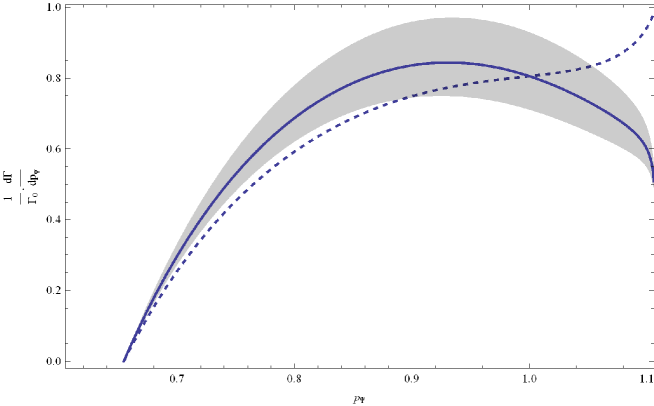
Figure 2: The decay rate $1/\Gamma_{0}\mathrm{d}\Gamma/\mathrm{d}p_{\psi}$ via QED process. The dashed curve is the tree level direct rate He:arXiv0911 . The solid line presents the interpolated resummed direct rate. The shaded band is obtained by varying the collinear scale from $\mu_{c}=m_{X}/\sqrt{2}$ to $\mu_{c}=\sqrt{2}m_{X}$, since the choice of scale could only be determined by a higher order calculation.

After resumming the spectrum shape softens near the end-point and is thus more consistent with experimental data Briere:2004prd .

IV Conclusion

In this work, we study the color-singlet QED process for $J/\psi$ production in $\Upsilon$ decay in the kinematic limit region. Since the NRQED breaks down ate this limit, we apply the SCET to study the spectrum. Our calculation consists of matching onto a color-singlet operator in SCET by integrating out the hard scale. Once the usoft modes are decoupled from the collinear modes using a field redefinition, we are able to show a factorization theorem for the differential decay rate, in which the decay rate can be factorized into a hard piece, a collinear jet function, and usoft functions. As pointed out by Ref. Rothstein:1997plb the usoft function in this case can be calculated, resulting in just a shift from the partonic to the physical endpoint.

By running the resulting rate from the hard scale $\mu_{H}$ to the collinear scale $\mu_{c}$, we sum the large Sudakov logarithms. Finally, we combine the SCET calculation with the leading order, color-singlet NRQED result to make a prediction for the color-singlet contribution via QED process to the differential decay rate spectrum over the entire allowed kinematic range.

References

• (1) G. T. Bodwin, E. Braaten and G. P. Lepage, Phys. Rev. D 51 1125 (1995).
• (2) M. E. Luke, A. V. Manohar and I. Z. Rothstein, Phys. Rev. D 61 074025 (2000).
• (3) G. T. Bodwin, E. Braaten and G. P. Lepage, Phys. Rev. D 46 1914 (1992).
• (4) E. Braaten and S. Fleming Phys. Rev. Lett 74 3327 (1995).
• (5) P. L. Cho and M. B. Wise, Phys. Lett. B 346 129 (1995); A. K. Leibovich, Phys. Rev. D 56 4412 (1997); M. Beneke and M. Kramer, Phys. Rev. D 55 5269 (1997); E. Braaten, B. A. Kniehl and J. Lee, Phys. Rev. D 62 094005 (2000).
• (6) T.Affolder et al. [CDF Collabortion], Phys. Rev. Lett. 85 2886 (2000).
• (7) R. A. Briere, et al, CLEO Collaboration, Phys. Rev. D 70 072001 (2004)
• (8) Shi-yuan Li, Qu-bing Xie and Qun Wang, Phys.Lett. B 482 65 (2000).
• (9) Kingman  Cheung, Wai-Yee Keung and Tzu Chiang Yuan, Phys.Rev. D 54 929 (1996).
• (10) Zhi-Guo He and Jian-Xiong Wang, [arXiv:0911.0139].
• (11) C. W. Bauer, S. Fleming and M. Luke, Phys. Rev. D 63 014006 (2001).
• (12) C. W. Bauer, S. Fleming, D. Pirjol and I. W. Stewart, Phys. Rev. D 63 114020 (2001).
• (13) C. W. Bauer and I. W. Stewart, Phys. Lett. B 516 134 (2001).
• (14) C. W. Bauer, D. Pirjol and I. W. Stewart, Phys. Rev. D 65 054022 (2002).
• (15) S. Fleming, A. K. Leibovich, and T. Mehen, Phys. Rev. D 68 094011 (2003).
• (16) S. Fleming, A. K. Leibovich, Phys. Rev. D 67 074035 (2003).
• (17) E. Braaten and Y. Q. Chen, Phys. Rev. D 54 3216 (1996).
• (18) C. Bobeth, B. Grinstein, and M. Savrov, Phys. Rev. D 77 074007 (2008).
• (19) I. Z. Rothstein and M. B. Wise, Phys. Lett. B 402 346 (1997); M. Beneke, I. Z. Rothstein and M. B. Wise, Phys. Lett.  B 408, 373 (1997).