Some aspects of color superconductivity: an introduction

Interdisciplinary Center for Theoretical Study and Department of Modern Physics, University of Science and Technology of China, Anhui 230026, People’s Republic of China

Abstract: A pedagogical introduction to color superconductivity in the weak coupling limit is given. The focus is on the basic tools of thermal field theory necessary to compute observables of color superconductivity. The rich symmetry structure and symmetry breaking patterns are analyzed on the basis of the Anderson-Higgs mechanism. Some techniques can also be applied for computing neutrino processes in compact stars. As an example, we show how to obtain the neutrino emissivity for Urca processes in neutron stars by computing the polarization tensor of the W-boson. We also illustrate how a spin-1 color superconducting phase generates an anisotropic neutrino emissions in compact stars.

Keywords: Quantum Chromodynamics, Color Superconductivity, Thermal Field Theory, Compact Stars, Neutrino Emission

1 What is color superconductivity?

Nowadays, superconductivity in a wide range of materials and superfluidity of Helium-3 can be generated with practical equipments in laboratories. It is well known that the underlying mechanism of all these ’super’ phenomena is the so-called Cooper paring of fermions (electrons in superconductors, fermionic ${}^{3}\mathrm{He}$ atoms in Helium superfluids) near the Fermi surface of the corresponding fermions. These phenomena are all of electromagnetic nature and at atomic level. In the regime of strong interaction where quarks and gluons are elementary particles described by quantum chromodynamics (QCD), a similar phenomena, the so called color superconductivity was first proposed in cold dense quark matter by Barrois [1], Bailin and Love [2], and further developed by many others (for reviews, see [3, 4, 5, 6, 7, 8, 9, 10, 11, 12, 13, 14]). However color superconducting quark matter cannot be produced in any laboratory in the foreseeable future. The reason is that this exotic phase of matter requires extremely high baryonic densities and relatively low temperatures. In nature, such conditions are only realized in the cores of cold compact stars, i.e. in relatively old remnants of supernova explosions.

In a color superconductor, quarks form Cooper pairs similarly to electrons in a normal superconductor or to fermionic ${}^{3}\mathrm{He}$ atoms in a Helium superfluid. Quarks carry color charges and interact via gluon exchange (the gluon is the QCD gauge boson). At very high baryonic densities the quark chemical potential $\mu$ is much larger than the QCD scale $\Lambda_{QCD}\sim 200\;\mathrm{MeV}$, the running coupling constant $\alpha_{S}(\mu)$ is thus small, because QCD is an asymptotically free theory for quarks and gluons. This was first shown by Gross, Politzer and Wilczek in 1973 [15, 16] and awarded the Nobel Prize in 2004 [17, 18]. In this case, the interaction between quarks is dominated by one-gluon exchange. As will be demonstrated explicitly at the end of this section there is an attractive channel in one-gluon exchange providing the binding agent for the quark Cooper pair. This is in contrast to normal superconductors where an electron Cooper pair is formed indirectly via electron-lattice interaction (direct electron-electron interaction is repulsive). In this sense color superconductivity is simpler than the normal one. In hadronic matter quarks are confined in color-neutral hadrons. Only at sufficiently high baryonic densities when these hadrons overlap and eventually free the quarks out of their hadronic domains, the quarks can move in much larger space-time volumes than the size of hadrons. This phenomenon is called deconfinement. It is expected to occur in the core of some compact stellar objects as neutron stars, where the baryonic densities are a few times larger than the nuclear matter saturation density $\rho_{0}\sim 0.14\;\mathrm{fm}^{-3}$, which corresponds to a quark chemical potential $\mu\sim 400-500\;\mathrm{MeV}$.

Since quarks are fermions, the Pauli exclusion principle does not allow two quarks to occupy the same quantum state. At zero temperature, they fill up states up to the so-called Fermi momentum $k_{F}$ (or the Fermi surface) above which all states are empty. Due to Pauli blocking, only quarks near the Fermi surface are able to interact and exchange momenta. The exchanged momenta in quark-quark scattering are of order $k_{F}$. In the ultra-relativistic limit, we have $E_{F}=\sqrt{k_{F}^{2}+m^{2}}\approx k_{F}\approx\mu$. We know that the quark density $\rho\sim k_{F}^{3}\approx\mu^{3}$, the high baryonic density means large Fermi momentum $k_{F}$ or chemical potential $\mu$. We will consider asymptotically large quark chemical potentials, $\mu\gg\Lambda_{QCD}$, the so-called weak coupling approach, which means high density and large mementum transfer. The weak coupling approach enables one to study the phenomena in a rigorous or well-controlled way. For reviews of the weak coupling appoach, see, for example, [5, 13]. The physical predictions of such an approach certainly have to be interpreted very carefully, since for realistic $\mu$ one has $\alpha_{s}(\mu)\sim 1$. But aided by the resummation methods, the perturbative analysis can be extrapolated even to realistic densities such as those in the cores of neutron stars [13]. Support also comes from the NJL model [19, 20], a simple effective theory of QCD without gluons but with a local four-quark interaction. It predicts color superconductivity also at moderate baryonic densities with gaps of order of $\phi\sim 100\;\mathrm{MeV}$, which matches the gap value extropolated from the weak coupling approach. Recently there are many developments in the NJL model [21, 22, 23, 24] and in the random matrix model [25, 26], a more rigorous effective model, to describe the color superconducting phase diagram.

So at high baryonic densities where the strong coupling constant is small, the single gluon exchange dominates the quark-quark scattering, as shown in Fig. (1), whose amplitude is proportional to

$$\sum\limits_{a=1}^{N_{c}^{2}-1}T_{a}^{ii^{\prime}}T_{a}^{jj^{\prime}} = -\frac{N_{c}+1}{4N_{c}}\left(\delta_{ii^{\prime}}\delta_{jj^{\prime}}-\delta_{ij^{\prime}}\delta_{i^{\prime}j}\right)$$ (1)

$$+\frac{N_{c}-1}{4N_{c}}\left(\delta_{ii^{\prime}}\delta_{jj^{\prime}}+\delta_{ij^{\prime}}\delta_{i^{\prime}j}\right)\;.$$

Here, $N_{c}=3$ is the number of colors and $T_{a}$ are generators of the $SU(3)_{c}$ gauge group. Here $T_{a}\equiv\lambda_{a}/2$ where $\lambda_{a}$ are the Gell-Mann matrices. The indices $i,j$ are the fundamental colors of two quarks in the incoming channel, while $i^{\prime},j^{\prime}$ their resprective colors in the outgoing channel, see Fig. (1). Interchanging two color indices in the incoming or outgoing channel changes the sign of the first term while the second term remains intact. The minus sign in front of the asymmetric term indicates that this channel is attractive, as it is similar to the Coulomb interaction between a negative electric charge and a positive one (the product of two charges is negative). This finding is crucial, as due to Cooper’s theorem any arbitrarily weak attractive interaction will destabilize the Fermi surface in favor of the formation of Cooper pairs. Since the pairs are of bosonic nature they will condense at sufficiently low temperatures into a Bose-Einstein condensate (in a more rigorous way, Cooper pairs are Bose-Einstein condensate in strong coupling limit).

In group theory, Eq. (1) corresponds to deducing the direct product of two triplets into one color antitriplet (anti-symmetric) and one color sextet (symmetric)

$$[3]_{c}\otimes[3]_{c} = [\bar{3}]_{c}^{a}\oplus[6]_{c}^{s}\;.$$ (2)

Now we illustrate how two triplets makes an anti-triplet. Denote $\psi_{i}$ the quark field following the $SU(3)$ transformation:

$$\psi^{\prime}_{i} = g_{ij}\psi_{j},$$ (3)

where $g$ is a $SU(3)$ element. An anti-triplet can be written by $\widetilde{\psi}_{k}=\epsilon_{ijk}\psi_{i}\psi_{j}$, which transforms as

$$\widetilde{\psi}^{\prime}_{k} = \epsilon_{ijk}\psi^{\prime}_{i}\psi^{\prime}_{j}$$ (4)

$$= \epsilon_{ijk}g_{ii^{\prime}}g_{jj^{\prime}}\psi_{i^{\prime}}\psi_{j^{\prime}}$$

$$= \delta_{k^{\prime}k}\epsilon_{ijk^{\prime}}g_{ii^{\prime}}g_{jj^{\prime}}\psi_{i^{\prime}}\psi_{j^{\prime}}$$

$$= g_{k^{\prime}l}g_{lk}^{\dagger}\epsilon_{ijk^{\prime}}g_{ii^{\prime}}g_{jj^{\prime}}\psi_{i^{\prime}}\psi_{j^{\prime}}$$

$$= g_{lk}^{\dagger}\mathrm{det}(g)\epsilon_{i^{\prime}j^{\prime}l}\psi_{i^{\prime}}\psi_{j^{\prime}}$$

$$= \widetilde{\psi}_{l}g_{lk}^{\dagger},$$

where we have used $\epsilon_{ijk^{\prime}}g_{ii^{\prime}}g_{jj^{\prime}}g_{k^{\prime}l}=\mathrm{det}(g)\epsilon_{i^{\prime}j^{\prime}l}$ and $\mathrm{det}(g)=1$. We see that the anti-symmetric diquark field $\widetilde{\psi}_{k}$ transforms like an anti-quark.

From the anti-symmetry of the attractive channel it follows that the two quarks in a Cooper pair must carry different colors. In addition to colors, quarks also come along with spin and flavor quantum numbers. Since the total wave function of a Cooper pair has to be anti-symmetric under the exchange of two quarks, the combined spin-flavor part has to be symmetric. This requirement will be used in the following section to classify various possible color superconducting phases.

Figure 1: One gluon exchange

2 Structure of diquark condensate

In this section we discuss the structure of diquark condensate [8, 27]. A diquark condensate is defined as an expectation value

$$\mathcal{M}=\left\langle\overline{\psi}_{c}\mathcal{O}\psi\right\rangle,$$ (5)

where $\psi$ is the quark field with all Dirac, color and flavor indices, $\overline{\psi}_{c}$ is its charge conjugate field defined by $\overline{\psi}_{c}=\psi^{T}C$ with the charge conjugate operator $C=i\gamma^{2}\gamma_{0}$. The operator $\mathcal{O}$ has Dirac, color and flavor parts:

$$\mathcal{O} = \mathcal{O}_{Dirac}\otimes\mathcal{O}_{color}\otimes\mathcal{O}_{flavor}.$$ (6)

The charge conjugate operator can be determined by transforming the Dirac equation of a fermion to that of an anti-fermion,

$$(p_{\mu}\gamma^{\mu}-m)\psi=0$$ (7)

$$\rightarrow \psi^{T}(p_{\mu}\gamma^{\mu T}-m)=0$$

$$\rightarrow \psi^{T}C(p_{\mu}C^{-1}\gamma^{\mu T}C-m)=0$$

$$\rightarrow \overline{\psi}_{c}(p_{\mu}C^{-1}\gamma^{\mu T}C-m)=0$$

$$\rightarrow \overline{\psi}_{c}(p_{\mu}\gamma^{\mu}+m)=0.$$

One can verify that $C=i\gamma^{2}\gamma_{0}$ satisfies $C^{-1}\gamma^{\mu T}C=-\gamma^{\mu}$ or $C\gamma^{\mu T}C=\gamma^{\mu}$ using $\gamma^{\mu T}=\gamma^{0},-\gamma^{1},\gamma^{2},-\gamma^{3}$ for $\mu=0,1,2,3$. Exploiting the anti-symmetric property of the fermionic quark fields, one finds

$$\mathcal{M} = \left\langle\overline{\psi}_{c}\mathcal{O}\psi\right\rangle=\left\langle\psi^{T}C\mathcal{O}\psi\right\rangle$$ (8)

$$= \left\langle\psi_{i}(C\mathcal{O})_{ij}\psi_{j}\right\rangle$$

$$= -\left\langle\psi_{j}(C\mathcal{O})_{ji}^{T}\psi_{i}\right\rangle=-\left\langle\psi^{T}(C\mathcal{O})^{T}\psi\right\rangle.$$

So the operator $C\mathcal{O}$ obeys

$$(C\mathcal{O})^{T}=-C\mathcal{O}.$$ (9)

This means that the operator $C\mathcal{O}$ is anti-symmetric under transposition. We can choose all three parts of $C\mathcal{O}$, i.e. Dirac, color and flavor parts, anti-symmetric or two of them symmetric and the third one anti-symmetric. In Tab. (1) a variety of choices to build up the operator $\mathcal{O}$ is given together with the corresponding symmetric properties under transposition.

Table 1: Symmetric properties of $\mathcal{O}$ under transposition. In the row of Dirac part, ’S’, ’P’, ’V’, ’A’, ’T’ means that the operator $C\mathcal{O}$ is a scalar, pseudo-scalar, vector, axial-vector and tensor, respectively. In the U(2) row, $\sigma_{i}$ are Pauli matrices, while in the U(3) row, $\lambda_{i}$ are Gell-Mann matrices.

	Anti-symmetric	Symmetric
Dirac (combined with $C$)	$\gamma_{5}$ 1 $\gamma^{\mu}\gamma_{5}$ S P V	$\gamma^{\mu}$ $\sigma^{\mu\nu}$ A T
U(2)	$\sigma_{2}$ singlet [1]	1, $\sigma_{1}$, $\sigma_{3}$ triplet [3]
U(3)	$\lambda_{2}$, $\lambda_{5}$, $\lambda_{7}$ anti-triplet [$\overline{3}$]	1, $\lambda_{1}$, $\lambda_{3}$, $\lambda_{4}$, $\lambda_{6}$, $\lambda_{8}$ sextet [6]

Now we show how to determine the parity of the condensate. Suppose under parity transformation $\mathcal{P}$, the field $\psi(t,\mathbf{x})$ changes as follows

$$\mathcal{P}\psi(t,\mathbf{x})\mathcal{P} = \eta\gamma_{0}\psi(t,-\mathbf{x})$$

$$\mathcal{P}\overline{\psi}(t,\mathbf{x})\mathcal{P} = \eta^{*}\overline{\psi}(t,-\mathbf{x})\gamma_{0},$$ (10)

where $\eta$ is a complex number. Then the conjugate fields transform as

$$\mathcal{P}\psi_{c}(t,\mathbf{x})\mathcal{P} = \eta_{c}\gamma_{0}\psi_{c}(t,-\mathbf{x})$$

$$\mathcal{P}\overline{\psi}_{c}(t,\mathbf{x})\mathcal{P} = \eta_{c}^{*}\overline{\psi}_{c}(t,-\mathbf{x})\gamma_{0}.$$ (11)

So the condensate transforms as

$$\mathcal{P}\overline{\psi}_{c}(t,\mathbf{x})\mathcal{O}\psi(t,\mathbf{x})\mathcal{P} = \eta_{c}^{*}\eta\overline{\psi}_{c}(t,-\mathbf{x})\gamma_{0}\mathcal{O}\gamma_{0}\psi(t,-\mathbf{x})$$ (12)

$$= -\overline{\psi}_{c}(t,-\mathbf{x})\gamma_{0}\mathcal{O}\gamma_{0}\psi(t,-\mathbf{x}),$$

where use was made of the fact that the parity of the conjugate particle is opposite to that of the particle, i.e. $\eta_{c}^{*}=-\eta$. Then $\mathcal{O}=\gamma_{5},1,\gamma^{\mu}\gamma_{5},\gamma^{\mu},\sigma^{\mu\nu}$ correspond to a scalar, pseudo-scalar, vector, pseudo-vector and tensor, respectively, as shown in the second row of Tab. (1). For example, $\mathcal{O}=\gamma^{\mu}\gamma_{5}$ gives a vector, since

$$\mathcal{P}\overline{\psi}_{c}(t,\mathbf{x})\gamma^{0}\gamma_{5}\psi(t,\mathbf{x})\mathcal{P} = \overline{\psi}_{c}(t,-\mathbf{x})\gamma^{0}\gamma_{5}\psi(t,-\mathbf{x}),$$

$$\mathcal{P}\overline{\psi}_{c}(t,\mathbf{x})\gamma^{i}\gamma_{5}\psi(t,\mathbf{x})\mathcal{P} = -\overline{\psi}_{c}(t,-\mathbf{x})\gamma^{i}\gamma_{5}\psi(t,-\mathbf{x}),$$ (13)

which transforms as a vector.

From spin-0 pairing (see, e.g. [19, 20, 27, 28]), we require that the color part is anti-symmetric with respect to exchanging two quarks, i.e. the color part is in the anti-triplet channel, and that the Dirac part must be a Lorentz scalar or pseudo-scalar, i.e. the Dirac part of $\mathcal{O}$ must be $\gamma_{5}$ or $1$ which is anti-symmetric combined with $C$. Therefore the flavor part should be anti-symmetric too, i.e. it must be a flavor singlet in the two-flavor case or a flavor anti-triplet in the three-flavor case. The condensate is then a $J^{P}=0^{+}$(spin-parity) or $J^{P}=0^{-}$ bound state of two quarks depending on whether the Dirac part is $\gamma_{5}$ or $1$. For the spin-1 pairing (see, e.g. [29, 30, 31, 32, 33, 34, 35, 36, 37]), the color part must be anti-triplet (anti-symmetric) and the Dirac part can be a vector (symmetric) or an axial-vector (anti-symmetric), so the flavor part can be symmetric or anti-symmetric respectively. There is another example for the spin-1 pairing in the single-color case where the color part is symmetric and flavor one anti-symmetric [38]. If the single flavor pairing occurs (the flavor part is symmetric), the Dirac part must be $\gamma^{\mu}$. Therefore a spin-1 Cooper pair is a $J^{P}=1^{-}$ state. Tab. (2) summarizes the structure of diquark condensates in spin-0 and spin-1 pairings.

Table 2: Structure of diquark condensates $\mathcal{M}$, the Dirac part is refered to that of the operator $\mathcal{O}$ (not that of $C\mathcal{O}$). $J^{P}$ is the spin-parity. Note that the color part is always in anti-triplet for all condensates.

pairing	Dirac part ($J^{P}$)	flavor multiplet (number of flavor)
spin-0	$\gamma_{5}$($0^{+}$),1 ($0^{-}$)	1 ($N_{f}=2$), $\overline{3}$ ($N_{f}=3$)
spin-1	$\gamma^{\mu}$ ($1^{-}$)	1 ($N_{f}=1$), 3 ($N_{f}=2$), 6 ($N_{f}=3$)
spin-1	$\gamma^{\mu}\gamma_{5}$ ($1^{+}$)	1 ($N_{f}=2$), $\overline{3}$ ($N_{f}=3$)

Generally the gap of a spin-0 pairing is much larger than that of a spin-1 pairing. In the ideal case there is more energy benefit for the spin-0 pairing compared to the spin-1 pairing, so the spin-0 pairing is favorable. But in the real world, there are many factors to disfavor the spin-0 pairing. For example, when electric neutrality is taken into account, there is a difference between the chemical potential of the strange quark and that of light quarks $u$ and $d$ due to the large strange quark mass. Additionally, the chemical potentials of $u$ and $d$ quarks differ due to $\beta$-equilibrium. If the differences of the chemical potentials are large enough, the spin-0 pairing, e.g. CFL phase, is not favorable [39, 40, 41, 42], and the spin-1 pairing or LOFF pairing [43] might be the true ground state [44, 45]. Another possibility to kill the spin-0 pairing is the presence of a strong magnetic field which favors the symmetric spin wave function [32].

3 Spontaneous symmetry breaking

A symmetry of the Lagrangian is said to be spontaneously broken if the ground state or the vacuum of the system is not invariant under the operations of that symmetry. We call this phenomenon spontaneous symmetry breaking.

A well-known example is the ferromagnetism arising from the spin-spin coupling, see Fig. (2). The Lagrangian describing the ferromagnetism is invariant with respect to a $SO(3)$ rotation. Above the transition temperature $T_{c}$, the vacuum state of the spin system is invariant with respect to $SO(3)$ rotation since the spin orientations are totally random and any rotation does not change the spin state macroscopically. Below $T_{c}$ the vacuum spontaneously chooses one magnetization direction, so the groud state is no longer invariant under $SO(3)$ rotation. The $SO(3)$ symmetry of the vacuum is spontaneously broken to $SO(2)$ which describes the rotational symmetry around the total spin direction. We thus write this symmetry breaking pattern as $G=SO(3)\rightarrow H=SO(2)$, where $G$ is the total symmetry and $H$ the residual symmetry.

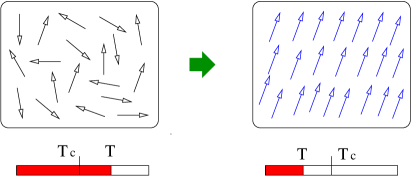
Figure 2: The ferromagnetism as an example of spontaneous symmetry breaking.

In the second example of spontaneous symmetry breaking the concept of the locking state is explained. Suppose we have a system composed of red and blue spins of $U(1)$ symmetry, see Fig. (3). Above a transition temperature $T_{c}$, the red and blue spin orientations are totally random. Below $T_{c}$, there are four possibilities of breaking the total symmetry spontaneously:

$$G=U(1)_{red}\otimes U(1)_{blue} \rightarrow H=U(1)_{blue}$$

$$G=U(1)_{red}\otimes U(1)_{blue} \rightarrow H=U(1)_{red}$$

$$G=U(1)_{red}\otimes U(1)_{blue} \rightarrow H=1$$

$$G=U(1)_{red}\otimes U(1)_{blue} \rightarrow H=U(1)_{red+blue}$$ (14)

In the first one the red spin symmetry is broken while the blue one remains. In the second one the blue spin symmetry is broken but the red one remains. In the third breaking pattern, both the red and blue spin symmetries are spontaneously broken. The fourth pattern is special in that both the red and blue spins point in any directions but their relative angle is fixed. This symmetry breaking pattern is called locking in the sense that the state is invariant under the joint rotation of the red and blue spins with the same rotational angle. The locking, for example, is the underlying mechanism for various phases in the superfluid Helium-3 [46].

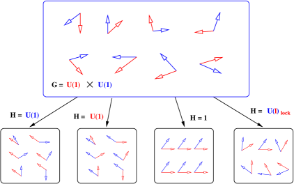
Figure 3: The locking state as an example of spontaneous symmetry breaking.

The well-known Nambu-Goldstone theorem [47, 48] states that the spontaneous breaking of a continuous global symmetry implies a massless spin zero or scalar particle, and that each broken generator of the symmetry group gives rise to one such particle. Consider the complex scalar field as an example. The potential can be written as

$$V(|\phi|^{2}) = a|\phi|^{2}+b|\phi|^{4},$$ (15)

where $a\sim a^{\prime}(T-T_{c})$ and $a^{\prime},b>0$, see Fig. (4). The above potential is invariant under $U(1)$ transformation, $\phi^{\prime}=e^{i\theta}\phi$. Above $T_{c}$ the potential exhibits a minimum at $\phi=0$ which is intact under $U(1)$ transformation. Below $T_{c}$ the potential is minimal along the circle with radius $|\phi|=\phi_{0}$, because the coefficient $a$ has different signs below and above $T_{c}$. The symmetry of $U(1)$ is spontaneously broken because the vacuum is changed after any $U(1)$ transformation $\phi^{\prime}=e^{i\theta}\phi=e^{i\theta^{\prime}}\phi_{0}$. One sees that below $T_{c}$ there is a massless mode (the so-called Goldstone mode) along the circle of minima.

A general proof of the Goldstone theorem can be given as follows. Suppose a given potential is invariant under the transformation of a continuous group:

$$\delta\Phi=i\theta^{a}C^{a}\Phi,$$ (16)

where $\Phi=[\phi_{1},\cdots,\phi_{n_{G}}]^{T}$ with $\phi_{i}$ being the real scalar field component and $n_{G}$ the number of real scalar fields. $C^{a}$ are operators of the corresponding Lie algebra of the group. The infinitesimal change of the potential due to $\delta\Phi$ should vanish

$$\delta V(\Phi) = \frac{\delta V}{\delta\phi_{i}}\delta\phi_{i}=i\frac{\delta V}{\delta\phi_{i}}\theta^{a}(C^{a})_{ij}\phi_{j}=0.$$ (17)

Since $\theta^{a}$ are arbitrary we have

$$\frac{\delta V}{\delta\phi_{i}}(C^{a})_{ij}\phi_{j} = 0$$ (18)

for $a=1,\cdots,n_{G}$. Taking an additional derivative with respect to $\phi_{k}$, we obtain

$$\frac{\delta^{2}V}{\delta\phi_{k}\delta\phi_{i}}(C^{a})_{ij}\phi_{j}+\frac{\delta V}{\delta\phi_{i}}(C^{a})_{ik} = 0.$$ (19)

Evaluating the above equation at the vacuum $\Phi=\Phi_{0}$, the second term vanishes, and we have

$$M_{ki}^{2}(C^{a})_{ij}\phi_{0j} = 0,$$ (20)

where the mass matrix is defined by $M_{ki}^{2}=\left.\frac{\delta^{2}V}{\delta\phi_{k}\delta\phi_{i}}\right|_{\Phi=\Phi_{0}}$. If the ground state is invariant under a sub-group $H$ of $G$, for each generator belonging to this sub-group $H$, we have

$$(C^{a})_{ij}\phi_{0j} = 0$$ (21)

for $a=1,\cdots,n_{H}$. For the remaining $n_{G}-n_{H}$ generators, we have

$$(C^{a})_{ij}\phi_{0j} \neq 0.$$ (22)

So Eq. (20) shows that there are $n_{G}-n_{H}$ zero eigenvalues for the mass matrix which means $n_{G}-n_{H}$ massless Goldstone bosons.

Note that the above argument holds for a Lorentz invariant system. In the context of dense quark matter where the Lorentz invariance is lost, the Nambu-Goldstone bosons have many fine structures, see, e.g. Ref. [49, 50, 51].

Figure 4: Potential for complex scalar field

\psfrag{potential}{$V(|\phi|^{2})$}\psfrag{Rephi}{Re($\phi$)}\psfrag{Imphi}{Im($\phi$)}\psfrag{TgreaterTc}{$T>T_{c}$}\psfrag{TlessTc}{$T<T_{c}$}\psfrag{massive}{\small massive}\psfrag{massless}{\small massless}\includegraphics[scale={0.8}]{china07}

4 Scalar QED as an example of superconductor

In the above section we discussed the spontaneous breaking of a global symmetry. In this section we will investigate the spontaneous breaking of a local gauge symmetry. We will show that it is also a good example for superconductivity. To this end, we consider a theory of a complex scalar and a U(1) gauge field where they couple to each other in a minimal way, the so-called scalar quantum electromagnetism or scalar QED. The Lagrangian is

$$\mathcal{L} = (D_{\mu}\phi)^{\dagger}D^{\mu}\phi-V(|\phi|^{2})-\frac{1}{4}F_{\mu\nu}F^{\mu\nu},$$ (23)

where the covariant derivative is defined by $D_{\mu}\equiv\partial_{\mu}+ieA_{\mu}$ and the guage field stength tensor by $F_{\mu\nu}\equiv\partial_{\mu}A_{\nu}-\partial_{\nu}A_{\mu}$. The potential is given by $V(|\phi|^{2})=\lambda(|\phi|^{2}-\phi_{0}^{2})$. The Lagrangian $\mathcal{L}$ is invariant under a U(1) local gauge transformation,

$$\phi^{\prime} = e^{ie\theta(x)}\phi,$$

$$A^{\prime}_{\mu} = A_{\mu}-\partial_{\mu}\theta.$$ (24)

One can verify that under the above transformation $D^{\prime}_{\mu}\phi^{\prime}=e^{ie\theta(x)}D_{\mu}\phi$. Therefore the term $(D_{\mu}\phi)^{\dagger}D^{\mu}\phi$ is invariant.

The Lagrangian equation for the gauge field reads

$$\partial^{\mu}F_{\mu\nu} = j_{\nu},$$

$$j_{\nu} = ie(\phi^{*}\partial_{\nu}\phi-\phi\partial_{\nu}\phi^{*})-2e^{2}|\phi|^{2}A_{\nu}.$$ (25)

The current $j_{\mu}$ satisfies the conservation law $\partial^{\mu}j_{\mu}=0$ due to $\partial^{\mu}\partial^{\nu}F_{\mu\nu}=0$. The Lagrangian equation for the scalar field reads

$$(\partial_{\mu}+ieA_{\mu})(\partial^{\mu}+ieA^{\mu})\phi = 2\lambda\phi(\phi_{0}^{2}-|\phi|^{2}).$$ (26)

In the covariant gauge $\partial_{\mu}A^{\mu}=0$ and choosing the real scalar field (unitary gauge) $\phi^{*}=\phi=\rho$, the equation for the gauge field becomes

$$(\partial^{\mu}\partial_{\mu}+2e^{2}\rho^{2})A_{\nu} = 0.$$ (27)

Suppose $\rho$ is very close to the vacuum value $\phi_{0}$, we can expand $\rho=\phi_{0}+\eta$, the linearized equation of motion for the scalar field become

$$(\partial^{\mu}\partial_{\mu}+4\lambda\phi_{0}^{2})\eta = 0,$$ (28)

where we have dropped higher order terms like $A^{\mu}\partial_{\mu}\eta$ and $A^{\mu}A_{\mu}$ etc..

5 Invariant subgroup for order parameter

Consider a symmetry group in a theory

$$G=G_{1}\otimes G_{2},$$ (29)

where $G_{1}$ and $G_{2}$ are Lie groups (a generalization to more than two groups is straightforward). The group elements can be expressed in terms of the generators of the respective Lie algebras

$$g = g_{1}\otimes g_{2}$$

$$g_{1} = e^{iC_{1}^{a}\theta_{1}^{a}}\in G_{1}$$

$$g_{2} = e^{iC_{2}^{a}\theta_{2}^{a}}\in G_{2},$$ (30)

where $C_{1}^{a}\;(a=1\cdots n_{1})$ and $C_{2}^{a}\;(a=1\cdots n_{2})$ are the generators of the Lie algebras $G_{1}$ and $G_{2}$, respectively. $\theta_{1}^{a}$ and $\theta_{2}^{a}$ are rotational angles associated with the operators $C_{1}^{a}$ and $C_{2}^{a}$ respectively.

Now we investigate how the order parameter changes under the transformation of the group $G$. After choosing one representation for the group $G$, the order parameter $\mathcal{M}$ can be written on its basis

$$\mathcal{M} \sim \Delta_{ij}\mathbf{e}_{1i}\otimes\mathbf{e}_{2j},$$ (31)

where the coefficient $\Delta_{ij}$ is the gap matrix, and $\mathbf{e}_{1i}$ and $\mathbf{e}_{2j}$ are basis vectors for $G_{1}$ and $G_{2}$ representations, respectively. After transformation, the order parameter becomes

$$\mathcal{M}^{\prime} = g_{1}\otimes g_{2}\mathcal{M}g_{1}^{T}\otimes g_{2}^{T}$$ (32)

$$\sim \Delta_{ij}g_{1}\mathbf{e}_{1i}g_{1}^{T}\otimes g_{2}\mathbf{e}_{2j}g_{2}^{T}.$$

For infinitesimal transformation

$$g_{1} \approx 1+iC_{1}^{a}\theta_{1}^{a}$$

$$g_{2} \approx 1+iC_{2}^{a}\theta_{2}^{a},$$ (33)

Eq. (32) becomes

$$\mathcal{M}^{\prime} = \mathcal{M}+i\theta_{1}^{a}\Delta_{ij}(C_{1}^{a}\mathbf{e}_{1i}+\mathbf{e}_{1i}C_{1}^{aT})\otimes\mathbf{e}_{2j}$$ (34)

$$+i\theta_{2}^{a}\Delta_{ij}\mathbf{e}_{1i}\otimes(C_{2}^{a}\mathbf{e}_{2j}+\mathbf{e}_{2j}C_{2}^{aT})$$

To find the invariant subgroup for the order parameter, we require $\mathcal{M}^{\prime}=\mathcal{M}$ and then

$$i\theta_{1}^{a}\Delta_{ij}(C_{1}^{a}\mathbf{e}_{1i}+\mathbf{e}_{1i}C_{1}^{aT})\otimes\mathbf{e}_{2j}$$

$$+i\theta_{2}^{a}\Delta_{ij}\mathbf{e}_{1i}\otimes(C_{2}^{a}\mathbf{e}_{2j}+\mathbf{e}_{2j}C_{2}^{aT})=0$$ (35)

From this equation we can find the subset of operators $C_{1,2}^{a}$ which make up the sub-algebra of the residual symmetry.

For the $SU(3)$ group, we have a simpler version of Eq. (35). We know that the color part of the order parameter is the anti-triplet. So the basis of the color part now should be $J_{i}$, the color anti-symmetric matrices defined by $(J_{i})_{jk}=i\epsilon_{jik}=-i\epsilon_{ijk}$. Now we look at $g_{1}J_{i}g_{1}^{T}$, where $g_{1}$ is a $SU(3)$ group element in fundamental representation (a 3 by 3 unitary matrix), which satisfies $g_{1}g_{1}^{\dagger}=1$ and $\mathrm{det}(g_{1})=1$. Using these properties we can simplify $g_{1}J_{i}g_{1}^{T}$ as

$$g_{1ji}[g_{1}J_{i}g_{1}^{T}]_{mn} = g_{1ji}g_{1ml}(J_{i})_{lp}g_{1np}$$ (36)

$$= -i\epsilon_{ilp}g_{1ji}g_{1ml}g_{1np}$$

$$= -i\epsilon_{jmn}\mathrm{det}(g_{1}).$$

Multiplying $(g_{1}^{\dagger})_{kj}$ on both sides, we get

$$[g_{1}J_{k}g_{1}^{T}]_{mn} = -i\epsilon_{jmn}(g_{1}^{\dagger})_{kj}$$ (37)

$$= (g_{1}^{\dagger})_{kj}(J_{j})_{mn},$$

or in operator form

$$g_{1}J_{k}g_{1}^{T} = (g_{1}^{\dagger})_{kj}J_{j}.$$ (38)

In the case of the $SU(2)$ group, for example, the number of flavors is 2, we will encounter $g_{1}\sigma_{2}g_{1}^{T}$, where $g_{1}$ is a $SU(2)$ group element in fundamental representation (a 2 by 2 unitary matrix). Using $g_{1}g_{1}^{\dagger}=1$ and $\mathrm{det}(g_{1})=1$, we have

$$[g_{1}\sigma_{2}g_{1}^{T}]_{mn} = g_{1ml}(\sigma_{2})_{lp}g_{1np}$$ (39)

$$= -i\epsilon_{lp}g_{1ml}g_{1np}$$

$$= -i\epsilon_{mn}\mathrm{det}(g_{1})$$

$$= (\sigma_{2})_{mn}$$

Therefore we obtain $g_{1}\sigma_{2}g_{1}^{T}=\sigma_{2}$.

We can also simplify $g_{2}\kappa_{j}g_{2}^{T}$ for $SO(3)_{J}$. Here $\kappa_{j}$ with $j=1,2,3$ are the basis for the spin triplet. Because $g_{2}$ is a group element of $SO(3)$, we have $g_{2}^{T}=g_{2}^{-1}$. Then we obtain

$$g_{2}\kappa_{j}g_{2}^{T} = g_{2}\kappa_{j}g_{2}^{-1}$$ (40)

$$\approx (1+i\theta_{2}^{m}\kappa_{m})\kappa_{j}(1-i\theta_{2}^{n}\kappa_{n})$$

$$\approx \kappa_{j}+i\theta_{2}^{m}\kappa_{m}\kappa_{j}-i\theta_{2}^{n}\kappa_{j}\kappa_{n}$$

$$= \kappa_{j}+i\theta_{2}^{m}i\epsilon_{mjl}\kappa_{l}$$

$$= \kappa_{j}-i\theta_{2}^{m}(J_{m})_{jl}\kappa_{l}$$

$$\rightarrow [e^{-i\theta_{2}^{m}J_{m}}]_{jl}\kappa_{l}=(g_{2}^{\dagger})_{jl}\kappa_{l}.$$

5.1 Symmetry patterns: 2SC phase

Our first example for the spin-0 pairing is the 2SC phase with $u$ and $d$ quarks. For simplicity we consider the positive parity channel, for the complete case, see, e.g., Eq. (9) in Ref. [14]. The order parameter for this color-flavor coupling phase can be written in the following form

$$\mathcal{M} = J_{i}\Delta_{ij}I_{j}\gamma_{5},$$ (41)

where $J_{i}$ is the color anti-symmetric matrices given by $(J_{i})_{jk}=i\epsilon_{jik}=-i\epsilon_{ijk}$. We can also express $J_{i}$ in terms of Gell-Mann matrices $J_{1}=\lambda_{7}$, $J_{2}=-\lambda_{5}$ and $J_{3}=\lambda_{2}$. $I_{i}$ are the flavor anti-symmetric matrices defined in the same way as $J_{i}$. The coefficient of the order parameter $\Delta_{ij}$ for 2SC is $\Delta_{ij}=\Delta\delta_{j3}\delta_{i3}$. Incorporating this expression for $\Delta_{ij}$ into Eq. (41), we obtain

$$\mathcal{M}_{2SC} = \Delta J_{3}\sigma_{2}\gamma_{5},$$ (42)

where $(\sigma_{2})_{ij}=(I_{3})_{ij}=-i\epsilon_{ij}$ with $i,j=1,2$.

The symmetry group for the 2SC phase is

$$G = G_{1}\otimes G_{2}\otimes G_{3},$$ (43)

where $G_{1}=SU(3)_{c}$ is the color group, $G_{2}=SU(2)_{f}$ the flavor group, and $G_{3}=U(1)_{B}$ the baryon number group. Note that the electromagnetism group $U(1)_{em}$ is a subgroup of $SU(2)_{f}$ and $U(1)_{B}$, since the electric charge satisfies

$$Q=\mathrm{diag}(Q_{u},Q_{d})=\mathrm{diag}(2/3,-1/3)=T_{3}+B/2,$$ (44)

where $B=1/3$ is the baryon number.

First we want to find the invariant subgroup of $SU(3)_{c}$ and $SU(2)_{f}$, so we can safely drop $G_{3}$ for simplification of the notation. The symmetry group now is

$$G=G_{1}\otimes G_{2}=SU(3)_{c}\otimes SU(2)_{f}.$$ (45)

The elements of $SU(3)_{c}$ and $SU(2)_{f}$ are

$$g = g_{1}\otimes g_{2}$$

$$g_{1} = e^{iT_{a}\theta_{1}^{a}}\in SU(3)_{c}$$

$$g_{2} = e^{i\sigma_{a}\theta_{2}^{a}}\in SU(2)_{f},$$ (46)

where $\sigma_{a}$ with $a=1,2,3$ are Pauli matrices. According to Eq. (32), we obtain

$$\mathcal{M}^{\prime} = g_{1}\otimes g_{2}\mathcal{M}g_{1}^{T}\otimes g_{2}^{T}$$ (47)

$$= \Delta\gamma_{5}g_{1}J_{3}g_{1}^{T}\otimes g_{2}\sigma_{2}g_{2}^{T}$$

$$= \Delta\gamma_{5}(g_{1}^{\dagger})_{3i}J_{i}\otimes\sigma_{2}$$

where we have used Eq. (38) and (39). By expanding $g_{1}$ and $g_{2}$ to the linear term of $\theta_{1}^{a}$ and $\theta_{2}^{a}$ respectively, and requiring $\mathcal{M}^{\prime}=\mathcal{M}$, we have

$$\theta_{1}^{a}(T_{a})_{3i}J_{i}\otimes\sigma_{2} = 0,$$ (48)

For $a=1,2,3$ Eq. (48) holds automatically, because elements on the third row of $T_{1},T_{2},T_{3}$ are zero. This means that there is freedom to choose any values of $\theta_{1}^{a}$ with $a=1,2,3$. For $a=4,5,6,7,8$, we have

$$\theta_{1}^{a}(T_{a})_{3i}J_{i} = (\theta_{1}^{4}+i\theta_{1}^{5})T_{7}-(\theta_{1}^{6}+i\theta_{1}^{7})T_{5}-\frac{2}{\sqrt{3}}\theta_{1}^{8}T_{2}$$ (49)

where we see that $\theta_{1}^{a}(T_{a})_{3i}J_{i}$ is not zero. Therefore to make Eq. (48) hold, $\theta_{1}^{a}$ must vanish. We see that the orginal $SU(3)_{c}$ symmetry is spontaneously broken to $SU(2)_{c}$ spanned by operators $T_{1}$, $T_{2}$ and $T_{3}$ as follows

$$SU(3)_{c}\otimes SU(2)_{f} \rightarrow SU(2)_{c}\otimes SU(2)_{f}.$$ (50)

In order to get the invariant $U(1)$ group for the order parameter, we consider the transfromation of $U(1)_{em}$ for electromagnetism in the flavor sector. The elements of $SU(3)_{c}$ and $U(1)_{em}$ are

$$g = g_{1}\otimes g_{2}$$

$$g_{1} = e^{iT_{a}\theta_{1}^{a}}\in SU(3)_{c}$$

$$g_{2} = e^{iQ\theta_{2}}\in U(1)_{em},$$ (51)

Eq. (35) becomes

$$-\theta_{1}^{a}(T_{a})_{3i}J_{i}\otimes\sigma_{2}+J_{3}\otimes\sigma_{2}\frac{\theta_{2}}{3}=0.$$ (52)

where we have used

$$[e^{iQ\theta}\sigma_{2}e^{iQ\theta}]_{kl} = -i\epsilon_{ij}[e^{iQ\theta}]_{ki}[e^{iQ\theta}]_{lj}$$ (53)

$$= -i\epsilon_{kl}\det[e^{iQ\theta}]$$

$$= \sigma_{2}e^{i(Q_{u}+Q_{d})\theta}=\sigma_{2}e^{i\theta/3}$$

The above equation becomes

$$\left[(-\theta_{1}^{4}-i\theta_{1}^{5})T_{7}+(\theta_{1}^{6}+i\theta_{1}^{7})T_{5}\right.$$

$$\left.+\frac{2}{\sqrt{3}}\theta_{1}^{8}T_{2}\right]\otimes\sigma_{2}+\frac{2}{3}\theta_{2}T_{2}\otimes\sigma_{2}=0.$$ (54)

We obtain

$$\theta_{1}^{a} = 0,\;\;a=4,5,6,7$$

$$\theta_{1}^{8} = -\frac{1}{\sqrt{3}}\theta_{2}.$$ (55)

With this relation between $\theta_{1}^{8}$ and $\theta_{2}$ we can combine the group elements as

$$e^{iT_{8}\theta_{1}^{8}}\otimes e^{iQ\theta_{2}}=e^{i\widetilde{Q}\theta_{2}},$$ (56)

with the new $\widetilde{U}(1)$ charge given by

$$\widetilde{Q}=1\otimes Q-\frac{1}{\sqrt{3}}T_{8}\otimes 1,$$ (57)

where $T_{8}=\frac{1}{2\sqrt{3}}\mathrm{diag}(1,1,-2)$. So the original symmetry is broken as

$$SU(3)_{c}\otimes U(1)_{em} \rightarrow SU(2)_{c}\otimes\widetilde{U}(1).$$ (58)

The $\widetilde{Q}$ charge in the 2SC phase for $u$ and $d$ quarks with different colors are listed in Tab. (3). We see that the condensate made of $(u_{1}d_{2},u_{2}d_{1})$ is $\widetilde{Q}$ neutral because $\widetilde{Q}_{cond}=\widetilde{Q}(u_{1})+\widetilde{Q}(d_{2})=\widetilde{Q}(u_{2})+\widetilde{Q}(d_{1})=0$.

Table 3: $\widetilde{Q}$ charge in 2SC and CFL phases. The colors are labelled by 1,2 and 3.

2SC	1	2	3
u	1/2	1/2	1
d	-1/2	-1/2	0

CFL	1	2	3
u	0	1	1
d	-1	0	0
s	-1	0	0

5.2 Symmetry pattern: CFL phase

Our second example for the spin-0 pairing CFL phase. For simplicity we consider the positive parity channel, for the full case, see, e.g., Eq. (6) in Ref. [14]. The order parameter can be written as

$$\mathcal{M} = J_{i}\Delta_{ij}I_{j}\gamma_{5}=\Delta\mathbf{J}\cdot\mathbf{I}\gamma_{5},$$ (59)

with $\Delta_{ij}=\Delta\delta_{ij}$. The symmetry group is

$$G = G_{1}\times G_{2}\times G_{3}=SU(3)_{c}\times SU(3)_{f}\times U(1)_{B}.$$ (60)

Now we try to find the invariant subgroup for the order parameter. We will see $U(1)_{B}$ plays no role, so we only $G_{1}$ and $G_{2}$ in the following discussion. Then the group elements are

$$g = g_{1}\otimes g_{2}$$

$$g_{1} = e^{iT_{a}\theta_{1}^{a}}\in SU(3)_{c}$$

$$g_{2} = e^{iT_{a}\theta_{2}^{a}}\in SU(3)_{f}.$$ (61)

Eq. (35) for the CFL phase becomes

$$\theta_{1}^{a}(T_{a})_{ij}J_{j}\otimes I_{i}$$

$$+\theta_{2}^{a}J_{i}\otimes(T_{a})_{ij}I_{j}=0.$$ (62)

We use following formula to simplify the above equation

$$\theta^{a}(T_{a})_{1j}J_{j} = (-\theta^{1}+i\theta^{2})T_{5}+(\theta^{4}-i\theta^{5})T_{2}$$

$$+(\theta^{3}+\frac{1}{\sqrt{3}}\theta^{8})T_{7}$$

$$\theta^{a}(T_{a})_{2j}J_{j} = (\theta^{1}+i\theta^{2})T_{7}+(\theta^{6}-i\theta^{7})T_{2}$$

$$+(\theta^{3}-\frac{1}{\sqrt{3}}\theta^{8})T_{5}$$

$$\theta^{a}(T_{a})_{3j}J_{j} = (\theta^{4}+i\theta^{5})T_{7}-(\theta^{6}+i\theta^{7})T_{5}$$ (63)

$$-\frac{2}{\sqrt{3}}\theta^{8}T_{2}$$

Then we obtain following conditions from Eq. (62)

$$\theta_{1}^{a} = \eta_{a}\theta_{2}^{a}$$ (64)

where $\eta_{a}=1$ for $a=2,5,7$ and $\eta_{a}=-1$ for $a=1,3,4,6,8$. We see that in order to make the order parameter invariant, we have to lock the rotaional angles for $SU(3)_{c}$ and $SU(3)_{f}$. The orginal symmetry $SU(3)_{c}\times SU(3)_{f}$ is broken to $SU(3)_{c+f}$.

To find the new $U(1)$ charge, we consider the transfromation of $U(1)_{em}$ in the flavor sector with the generator of $U(1)_{em}$ given by

$$Q = \left(\begin{array}[]{ccc}Q_{u}&0&0\\ 0&Q_{d}&0\\ 0&0&Q_{s}\end{array}\right)=\left(\begin{array}[]{ccc}2/3&0&0\\ 0&-1/3&0\\ 0&0&-1/3\end{array}\right).$$ (71)

Note that $U(1)_{em}$ is a subgroup of $SU(3)_{f}$ since $Q=T_{3}+T_{8}/\sqrt{3}$. We use

$$[e^{iQ\theta}]_{ii^{\prime}}[e^{iQ\theta}J_{i^{\prime}}e^{iQ\theta}]_{kl} = -i\epsilon_{i^{\prime}mn}[e^{iQ\theta}]_{ii^{\prime}}[e^{iQ\theta}]_{km}[e^{iQ\theta}]_{ln}$$ (72)

$$= -i\epsilon_{ikl}\det[e^{iQ\theta}]$$

$$= J_{i}e^{i(Q_{u}+Q_{d}+Q_{s})\theta}=J_{i}$$

to obtain

$$e^{iQ\theta}J_{i}e^{iQ\theta} = e^{-iQ\theta}J_{i}.$$ (73)

Then we derive the equation for determing the residue symmetry

$$\theta_{1}^{a}(T_{a})_{ij}J_{j}\otimes I_{i}+\theta_{2}J_{i}\otimes Q_{ii}I_{i}=0.$$ (74)

Finally we obtain following conditions

$$\theta_{1}^{a} = 0,\;\;a\neq 3,8$$

$$\theta_{1}^{3} = -\theta_{2}$$

$$\theta_{1}^{8} = -\frac{1}{\sqrt{3}}\theta_{2}.$$ (75)

We can rewrite the group element as

$$e^{iT_{3}\theta_{1}^{3}+iT_{8}\theta_{1}^{8}}\otimes e^{iQ\theta_{2}}=e^{i\widetilde{Q}\theta_{2}},$$ (76)

where the new $U(1)$ charge is

$$\widetilde{Q} = 1\otimes Q-\left(T_{3}+\frac{1}{\sqrt{3}}T_{8}\right)\otimes 1$$ (77)

The $\widetilde{Q}$ charge in the CFL phase for $u$, $d$ and $s$ quarks with different colors are listed in Tab. (3). One can check that the condensate made of $(u_{1}d_{2},u_{2}d_{1})$, $(d_{2}s_{3},d_{3}s_{2})$ and $(s_{3}u_{1},s_{1}u_{3})$ is neutral because

$$\widetilde{Q}_{cond} = \widetilde{Q}(u_{1})+\widetilde{Q}(d_{2})=\widetilde{Q}(u_{2})+\widetilde{Q}(d_{1})$$ (78)

$$= \widetilde{Q}(d_{2})+\widetilde{Q}(s_{3})=\widetilde{Q}(d_{3})+\widetilde{Q}(s_{2})$$

$$= \widetilde{Q}(s_{3})+\widetilde{Q}(u_{1})=\widetilde{Q}(s_{1})+\widetilde{Q}(u_{3})=0.$$

5.3 Symmetry pattern: spin-1 phases

The condensate of spin-1 CSC transforms as an anti-triplet under $SU(3)_{c}$ transformation, and as a vector under spatial $SO(3)$ rotation. It carries a $U_{b}(1)$ charge of the baryon number. The symmetry group of the theory is then $G=SU(3)_{c}\times U_{b}(1)\times SO(3)$. The condensate can be written as $\mathcal{M}=\Delta_{ai}J_{a}\otimes\gamma^{i}$, where $\gamma^{i}$ with $i=1,2,3$ are Dirac matrices. The order parameter $\Delta_{ai}$ is a complex matrix of $3\times 3$ dimension and transforms as, $\Delta\rightarrow g_{1}\Delta g_{2}$, where $g_{1}\in U(3)\equiv SU(3)_{c}\times U_{b}(1)$ and $g_{2}\in SO(3)$. This can be seen by the transformation of the condensate,

$$\Delta_{ai}J_{a}\otimes\gamma^{i} \rightarrow \Delta_{ai}g_{1}J_{a}g_{1}^{T}\otimes g_{2}\gamma^{i}g_{2}^{T}=\Delta_{ai}J_{b}(g_{1})_{ba}\otimes(g_{2})_{ij}\gamma^{j}$$ (79)

$$=[(g_{1})_{ba}\Delta_{ai}(g_{2})_{ij}]J_{b}\otimes\gamma^{j}.$$

Here $g_{2}=\exp(i\frac{1}{2}\epsilon_{ijk}\theta_{k}\gamma^{i}\gamma^{j})$ in $g_{2}\gamma^{i}g_{2}^{T}$ is the $SO(3)$ representation in Dirac space and $g_{2}=\exp(i\theta_{k}J_{k})$ in $(g_{2})_{ij}\gamma^{j}$ is the $SO(3)$ representation in vector space. By a suitable transformation, $\Delta$ can be cast into the following form, $\Delta=S+iA$, where $S$ and $A$ are real symmetric and anti-symmetric matrices respectively. Since orthogonal rotation does not change the symmety of $S$ and $A$, they can be after transformation written in the form $S=\mathrm{diag}(\Delta_{1},\Delta_{2},\Delta_{3})$ and $A_{ij}=\epsilon_{ijk}\omega_{k}$, where $\Delta_{i},\omega_{i}$ are real numbers. The condensate then has the form,

$$\Delta=\left(\begin{array}[]{ccc}\Delta_{1}&i\omega_{3}&-i\omega_{2}\\ -i\omega_{3}&\Delta_{2}&i\omega_{1}\\ i\omega_{2}&-i\omega_{1}&\Delta_{3}\end{array}\right).$$ (80)

Generally a complex matrix has 18 real parameters, 12 of which can be fixed by a transformation of symmetry group $G$. We can classify the order parameter $\Delta$ by its invariant subgroups of $G$, which can be found by looking for $g_{1}$ and $g_{2}$ satisfying $g_{1}g_{2}^{T}\Delta g_{2}=\Delta$, which is equivalent to $g_{1}\Delta=\Delta$ and $g_{2}^{T}\Delta g_{2}=\Delta$. Since the matrix $A$ defines a vector $\overrightarrow{\omega}=\omega_{i}\mathbf{e}_{i}$, $A$ is invariant under a rotation $g_{2}=e^{iJ_{i}\theta_{2}^{i}}\in SO(3)$ with the axis in the direction of $\overrightarrow{\omega}$, i.e. $\overrightarrow{\theta_{2}}\parallel\overrightarrow{\omega}$, i.e. $g_{2}^{T}Ag_{2}=A$. One can verify that the same rotation $g_{2}$ also makes $S$ invariant if $S$ is in the form,

$$S_{ij}=c_{1}\delta_{ij}+c_{2}\left(\delta_{ij}-\frac{\omega_{i}\omega_{j}}{|\overrightarrow{\omega}|^{2}}\right),$$ (81)

To see that we note that $M_{i}\omega_{i}\omega_{j}\omega_{k}=0$. The $U(3)$ invariant subgroup whose element $g_{1}$ satisfies $g_{1}\Delta=\Delta$ is determined by the number of zero modes of $\Delta$. The subgroup is then $U(n)$ for the case of $n$ zero modes of $\Delta$. The classification of the order parameters is listed in Tab. 4, see [34, 36].

order parameter	unbroken symmetry	name
$\begin{pmatrix}\Delta_{1}&+ia&0\\ -ia&\Delta_{1}&0\\ 0&0&\Delta_{2}\end{pmatrix}$	$SO(2)_{v}$	oblate
$\begin{pmatrix}\Delta&+ia&0\\ -ia&\Delta&0\\ 0&0&0\end{pmatrix}$	$SO(2)_{v}\times U(1)_{L}$	cylindrical
$\begin{pmatrix}\Delta_{1}&+i\Delta_{1}&0\\ -i\Delta_{1}&\Delta_{1}&0\\ 0&0&\Delta_{2}\end{pmatrix}$	$SO(2)_{v}\times U(1)_{L}$	$\varepsilon$
$\begin{pmatrix}1&+i&0\\ -i&1&0\\ 0&0&0\end{pmatrix}$	$SU(2)_{L}\times SO(2)_{v}\times U(1)_{L}$	A
$\begin{pmatrix}1&0&0\\ 0&1&0\\ 0&0&1\end{pmatrix}$	$SO(3)_{v}$	CSL
$\begin{pmatrix}0&0&0\\ 0&0&0\\ 0&0&1\end{pmatrix}$	$SU(2)_{L}\times SO(2)_{R}\times U(1)_{L}$	polar
$\begin{pmatrix}0&0&0\\ z_{1}&z_{2}&z_{3}\\ z_{4}&z_{5}&z_{6}\end{pmatrix}$	$U(1)_{L}$	$N_{1}$
$\begin{pmatrix}0&0&0\\ 0&0&0\\ z_{1}&z_{2}&z_{3}\end{pmatrix}$	$SU(2)_{L}\times U(1)_{L}$	$N_{2}$
$\begin{pmatrix}\Delta_{1}&0&0\\ 0&\Delta_{1}&0\\ 0&0&\Delta_{2}\end{pmatrix}$	$SO(2)_{v}$	axial
$\begin{pmatrix}1&0&0\\ 0&1&0\\ 0&0&0\end{pmatrix}$	$SO(2)_{v}\times U(1)_{L}$	planar

Table 4: Classification and the symmetry breaking patterns of the order parameters, see Fig.1 of [34, 36]. L/R denote the transformation matrix acting on the left/right hand side of the condensate, while $SO(2)_{v}$ denotes the transformation that acts on both right and left hand side of the condensate.

We take a few examples. For the oblate phase, one can verify that the order parameter has $SO(2)$ residue symmetry, $g_{2}^{T}\Delta g_{2}=\Delta$, for $g_{2}(oblate)=e^{iJ_{3}\theta_{2}^{3}}$. Note that $\det\Delta\neq 0$, so there is no residue symmetry inherited from $U(3)$. For the cylindrical phase, the residue symmetry is $SO(2)\times U(1)$, whose transformation is

$$g_{1}=\mathrm{diag}(1,1,e^{i\theta}),\;g_{2}=e^{iJ_{3}\theta_{2}^{3}}.$$ (82)

Note that there is one zero eigenvalue for $\Delta$ so the invariant subgroup is $U(1)$. For the CSL phase, the residue symmetry is $SO(3)$, whose transformation matrix obeying $g_{2}^{T}\Delta g_{2}=\Delta$ is any rotational matrix since $\Delta$ is a unit matrix, i.e. $g_{2}(CSL)=e^{iJ_{i}\theta_{2}^{i}}$ with $i=1,2,3$.

A more convenient way of looking for invariant subgroup is by using infinitesimal transformation,

$$\Delta = g_{1}\Delta g_{2}=(1+i\theta+iT^{a}\theta_{1}^{a})\Delta(1+iJ_{i}\theta_{2}^{i})$$ (83)

$$\approx \Delta+i\theta\Delta+i\theta_{1}^{a}T^{a}\Delta+i\theta_{2}^{i}\Delta J_{i},$$

which requires

$$\theta\Delta+\theta_{1}^{a}T^{a}\Delta+\theta_{2}^{i}\Delta J_{i}=0$$ (84)

for any subset of non-vanishing angles $\theta$, $\theta_{1}^{a}$ and $\theta_{2}^{i}$.

We analyze a few phases. The forms of order parameters $\Delta$ are listed in Tab 4. (1) The oblate phase. Since $J_{3}\Delta=\Delta J_{3}$, we obtain the only non-vansihing angles are $\theta_{1}^{2}$ and $\theta_{1}^{3}$ and obey $\theta_{1}^{2}=-2\theta_{2}^{3}$. So we have verified that the invariant subgroup is $SO(2)$, whose generator is $2T^{2}\otimes 1-1\otimes J_{3}^{T}$. (2) The cylindrical phase. We have $\theta_{1}^{8}=-2\sqrt{3}\theta$ and $\theta_{1}^{2}=-2\theta_{2}^{3}$, which corresponds to residue symmetry $SO(2)\times U(1)$. The unbroken generators are $2T^{2}\otimes 1-1\otimes J_{3}^{T}$ for $SO(2)$ and $-\frac{1}{2\sqrt{3}}+T^{8}$ for $U(1)$. (3) The $\varepsilon$ phase. We obtain $\theta_{1}^{2}=-2\theta_{2}^{3}$ for $SO(2)$ and $(\theta=\frac{1}{3}\theta_{1}^{2},\theta_{1}^{8}=\frac{1}{\sqrt{3}}\theta_{1}^{2})$ for $U(1)$. The invariant generators are $2T^{2}\otimes 1-1\otimes J_{3}^{T}$ for $SO(2)$ and $\frac{1}{3}+T^{2}+\frac{1}{\sqrt{3}}T^{8}$ for $U(1)$ (to see this one can verify that the generator behaves like a projector). (4) The A phase. It is a special case of the cylindrical phase. We obtain $\theta_{1}^{2}=-2\theta_{2}^{3}$ for $SO(2)$ and $\theta_{1}^{8}=-2\sqrt{3}\theta$ for $U(1)$, whose generators are $2T^{2}\otimes 1-1\otimes J_{3}^{T}$ and $-\frac{1}{2\sqrt{3}}+T^{8}$ respectively. Additionally we have $\theta_{1}^{1}=-i\theta_{1}^{3}$, $\theta_{1}^{2}=\frac{1}{\sqrt{3}}\theta_{1}^{8}$ and $\theta_{1}^{4}=i(\theta_{1}^{6}-\theta_{1}^{5})-\theta_{1}^{7}$ for $SU(2)$, whose generators are $\frac{1}{2\sqrt{2}}(\frac{1}{\sqrt{3}}T^{2}+T^{8})$, $\frac{\sqrt{3}}{4}(T^{5}+T^{6})$, and $\frac{1}{2\sqrt{2}}(T^{7}-T^{4})$. It is more convenient to transform the order parameter $\Delta$ which is Hermitian in Tab 4 by a unitary matrix $\mathcal{U}$ into,

$$\Delta=\left(\begin{array}[]{ccc}0&0&0\\ 0&0&0\\ 1&i&0\end{array}\right)=\frac{1}{\sqrt{2}}\mathcal{U}\left(\begin{array}[]{ccc}1&i&0\\ -i&1&0\\ 0&0&0\end{array}\right),\;\mathcal{U}=\frac{1}{\sqrt{2}}\left(\begin{array}[]{ccc}0&0&-\sqrt{2}\\ i&1&0\\ 1&i&0\end{array}\right).$$ (85)

It is easy to check that the unbroken generators are, $T^{i}$ with $i=1,2,3$ for $SU(2)$, $\frac{1}{\sqrt{3}}+T^{8}=\frac{\sqrt{3}}{2}P_{12}$ for $U(1)$, and $1+J_{3}$ for $SO(2)$. Here we define $P_{12}=\mathrm{diag}(1,1,0)$ and $P_{3}=\mathrm{diag}(0,0,1)$. (5) The polar phase. The unbroken generators are $T^{i}$ with $i=1,2,3$ for $SU(2)$, $\frac{1}{\sqrt{3}}+T^{8}=\frac{\sqrt{3}}{2}P_{12}$ for $U(1)$, and $J_{3}$ for $SO(2)$. For more comprehensive analysis of symmetry breaking features of the spin-1 pairings, see [34, 36, 37].

5.4 More physics related to symmetry patterns

There are a lot of interesting phenomena arising from symmetry patterns in color superconductivity. For example, the new $U(1)$ charge corresponds to the new photon in some superconducting phases, which resembles $W^{\pm}$ and $Z^{0}$ bosons in electroweak theory, see Tab. (5) for the comparison between the electroweak theory and color superconductivity. One can do electroweak physics with the new photon [52, 53]. In presence of the new photon, magnetic fields show a special behavior in the neutron star core [54]. One can study the transimission and reflection of the new photon at the interface between different phases to reveal its connection to confinement [55]. Especially the new photon in the CFL phase can propagate in the color superconductor. Therefore the external magnetic field can penetrate the color superconducting quark core modifying the gap structure [56, 57], and producing different phases with different symmetries and low-energy physics [58, 59]. Another interesting thing related to the residual $SU(2)_{c}$ symmetry in the 2SC phase is that one can construct $SU(2)_{c}$ effective theory, where the elementary excitation is the glueball [60]. Through decaying to photons these glueballs can be possible source of Gamma Ray Burst [61].

Table 5: Comparison to the standard model.

	Weinberg-Salam	CSC with $N_{f}=2,3$
group	$SU(2)\times U(1)$ isospin, hypercharge	$SU(3)_{c}\times U(1)_{em}$ color, electromagnetism
field	$W_{1},W_{2},W_{3},W_{0}$	$A_{1},\cdots,A_{8},A$ gluons, photon
coupling constant	$g,g^{\prime}$	$g,e$
symmetry breaking	$SU(2)\times U(1)$ $\rightarrow U(1)_{em}$	$SU(3)_{c}\times U(1)_{em}$ $\rightarrow\widetilde{U}(1)$
new field	$W^{+},W^{-},Z^{0},A$	$A_{1},\cdots,A_{7},\widetilde{A}_{8},\widetilde{A}$
new coupling constant	$e=g^{\prime}\cos\theta_{W}$	$\widetilde{e}=e\cos\theta$
massless field	$A$	$\widetilde{A}$

6 Deriving the gap equation

In the above symmetry analysis it was demonstrated that a multitude of phases are possible when quarks form Cooper pairs. To decide which of those will be favorable at given $T$ and $\mu$ one has to determine the phase with the largest pressure. Generally, the pressure will grow with the gain of condensation energy of the Cooper pairs. This in turn will depend on the magnitude of the respective color superconducting order or gap parameters. In this section we will derive the QCD gap equation and solve it in the weak coupling limit.

We will use units in which $\hbar=c=k_{B}=1$. We denote a 4-vector by capital letters, $X^{\mu}=(x_{0},\mathbf{x})$, with $\mathbf{x}$ being a 3-vector of modulus $|\mathbf{x}|\equiv x$ and direction $\widehat{\mathbf{x}}\equiv\mathbf{x}/x$. For the summation over Lorentz indices, we use a notation familiar from Minkowski space, with metric $g^{\mu\nu}=\mathrm{diag}(+,-,-,-)$, although we exclusively work in compact Euclidean space-time with volume $V/T$, where $V$ is the 3-volume and $T$ the temperature of the system. Space-time integrals are denoted as $\int_{0}^{1/T}d\tau\int_{V}d^{3}\mathbf{x}\equiv\int_{X}$.

The partition function for QCD in absence of external sources reads

$$\mathcal{Z} = \int\mathcal{D}A\,\exp\left\{S_{A}[A]\right\}\,\mathcal{Z}_{q}[A]\;.$$ (86)

Here the (gauge-fixed) gluon action is

$$S_{A}[A] = \int_{X}\left[-\frac{1}{4}F_{a}^{\mu\nu}(X)\,F_{\mu\nu}^{a}(X)\right]+S_{gf}[A]+S_{ghost}[A]\;,$$ (87)

where $F_{\mu\nu}^{a}=\partial_{\mu}A_{\nu}^{a}-\partial_{\nu}A_{\mu}^{a}+gf^{abc}A_{\mu}^{b}A_{\nu}^{c}$ is the gluon field strength tensor, $S_{gf}$ is the gauge-fixing part, and $S_{ghost}$ the ghost part of the action.

The partition function for quarks in presence of gluon fields is

$$\mathcal{Z}_{q}[A] = \int\mathcal{D}\overline{\psi}\,\mathcal{D}\psi\,\exp\left\{S_{q}[A,\overline{\psi},\psi]\right\}\,\,,$$ (88)

where the quark action is

$$S_{q}[A,\overline{\psi},\psi] = \int_{X}\overline{\psi}(X)\,\left(i\gamma_{\mu}D_{X}^{\mu}+\mu\gamma_{0}-m\right)\,\psi(X)\,\,,$$

with the covariant derivative $D_{X}^{\mu}=\partial_{X}^{\mu}-igA_{a}^{\mu}(X)T_{a}$. Note that we focus on a single chemical poteintial and a single mass for simplicity. In fermionic systems at nonzero density, it is advantageous to additionally introduce charge-conjugate fermionic degrees of freedom,

$$\psi_{C}(X) = C\overline{\psi}^{T}(X)$$

$$\overline{\psi}_{C}(X) = \psi^{T}(X)C$$

$$\psi(X) = C\overline{\psi}_{C}^{T}(X)$$

$$\overline{\psi}(X) = \psi_{C}^{T}(X)C$$ (89)

where the charge-conjugation matrix satisfies $C^{-1}=C^{\dagger}=C^{T}=-C$, $C^{-1}\gamma_{\mu}^{T}C=-\gamma_{\mu}$. We may then rewrite the quark action in the form

$$S_{q}[A,\overline{\Psi},\Psi] = \frac{1}{2}\int_{X,Y}\overline{\Psi}(X)\,\mathcal{G}_{0}^{-1}(X,Y)\,\Psi(Y)$$ (90)

$$+\frac{g}{2}\int_{X}\overline{\Psi}(X)\,\hat{\Gamma}_{a}^{\mu}A_{\mu}^{a}(X)\,\Psi(X)\,\,,$$

where we defined the Nambu-Gor’kov quark spinors

$$\Psi\equiv\left(\begin{array}[]{c}\psi\\ \psi_{C}\end{array}\right),\;\;\;\overline{\Psi}\equiv(\overline{\psi},\overline{\psi}_{C})\,\,,$$

and the free inverse quark propagator in the Nambu-Gor’kov basis

$$\mathcal{G}_{0}^{-1}(X,Y) = \left(\begin{array}[]{cc}[G_{0}^{+}]^{-1}(X,Y)&0\\ 0&[G_{0}^{-}]^{-1}(X,Y)\end{array}\right)\,\,,$$

with the free inverse propagator for quarks and charge-conjugate quarks

$$[G_{0}^{\pm}]^{-1}(X,Y) \equiv (i\gamma_{\mu}\partial_{X}^{\mu}\pm\mu\gamma_{0}-m)\,\delta^{(4)}(X-Y)\,\,,$$

The quark-gluon vertex in the Nambu-Gor’kov basis is defined as

$$\hat{\Gamma}_{a}^{\mu} \equiv \left(\begin{array}[]{cc}\gamma^{\mu}T_{a}&0\\ 0&-\gamma^{\mu}T_{a}^{T}\end{array}\right)\,\,.$$ (95)

The factors $1/2$ in Eq. (90) compensate the doubling of quark degrees of freedom in the Nambu-Gor’kov basis.

As we shall work in momentum space, we Fourier-transform all fields, as well as the free inverse quark propagator. Since space-time is compact, energy-momentum space is discretized, with sums $(T/V)\sum_{K}\equiv T\sum_{n}(1/V)\sum_{\mathbf{k}}$. For a large volume $V$, the sum over 3-momenta can be approximated by an integral, $(1/V)\sum_{\mathbf{k}}\simeq\int d^{3}\mathbf{k}/(2\pi)^{3}$. For bosons, the sum over $n$ runs over bosonic Matsubara frequencies $\omega_{n}^{\mathrm{b}}=2n\pi T$, while for fermions, it runs over fermionic Matsubara frequencies $\omega_{n}^{\mathrm{f}}=(2n+1)\pi T$. In our Minkowski-like notation for four-vectors, $x_{0}\equiv t\equiv-i\tau$, $k_{0}\equiv-i\omega_{n}^{\mathrm{b}/\mathrm{f}}$. The 4-dimensional delta-function is conveniently defined as $\delta^{(4)}(X)\equiv\delta(\tau)\delta^{(3)}(\mathbf{x})=-i\delta(x^{0})\delta^{(3)}(\mathbf{x})$. The Fourier transformations for the fields and free inverse quark propagator are given by

$$\Psi(X) = \frac{1}{\sqrt{V}}\sum_{K}e^{-iK\cdot X}\,\Psi(K)\,\,,$$

$$\overline{\Psi}(X) = \frac{1}{\sqrt{V}}\sum_{K}e^{iK\cdot X}\,\overline{\Psi}(K)\,\,,$$

$$\mathcal{G}_{0}^{-1}(X,Y) = \frac{T^{2}}{V}\sum_{K,Q}e^{-iK\cdot X}\,e^{iQ\cdot Y}\,\mathcal{G}_{0}^{-1}(K,Q)\,\,,$$

$$A_{a}^{\mu}(X) = \frac{1}{\sqrt{TV}}\sum_{P}e^{-iP\cdot X}\,A_{a}^{\mu}(P)\,\,.$$ (96)

The normalization factors are chosen such that fields in momentum space are dimensionless. The free inverse quark propagator is diagonal in momentum space, too,

$$\mathcal{G}_{0}^{-1}(K,Q) = \frac{1}{T}\left(\begin{array}[]{cc}[G_{0}^{+}]^{-1}(K)&0\\ 0&[G_{0}^{-}]^{-1}(K)\end{array}\right)\delta_{K,Q}^{(4)}\,\,,$$ (99)

where $[G_{0}^{\pm}]^{-1}(K)\equiv\gamma_{\mu}K^{\mu}\pm\mu\gamma_{0}-m$.

Due to the relations (89), the charge-conjugate quark field in momentum space is related to the original field via $\psi_{C}(K)=C\overline{\psi}^{T}(-K)$ and $\overline{\psi}_{C}(K)=\psi^{T}(-K)C$. The measure of the functional integral over quark fields can then be rewritten in the form

$$\mathcal{D}\overline{\psi}\,\mathcal{D}\psi \equiv \prod_{K}d\overline{\psi}(K)\,d\psi(K)$$ (100)

$$= \mathcal{N}\prod_{(K,-K)}d\overline{\psi}(K)\,d\psi(K)\,d\overline{\psi}(-K)\,d\psi(-K)$$

$$= \mathcal{N}^{\prime}\prod_{(K,-K)}d\overline{\psi}(K)\,d\psi(K)\,d\overline{\psi}_{C}(K)\,d\psi_{C}(K)$$

$$= \mathcal{N}^{\prime\prime}\prod_{(K,-K)}d\overline{\Psi}(K)\,d\Psi(K)\equiv\mathcal{D}\overline{\Psi}\,\mathcal{D}\Psi\,\,,$$

with the constant normalization factors $\mathcal{N}$, $,\mathcal{N}^{\prime}$ and $\mathcal{N}^{\prime\prime}$. The last identity has to be considered as a definition for the expression on the right-hand side.

Figure 5: $\Gamma_{2}$ is the sum of all QCD two-particle irreducible vacuum diagrams. Here, only the two-loop contributions are shown explicitly. Wavy lines correspond to gluon propagation and straight lines to quark propagation.

Inserting Eqs. (96) - (100) into Eq. (88), the partition function for quarks becomes

$$\mathcal{Z}_{q}[A] = \int\mathcal{D}\overline{\Psi}\,\mathcal{D}\Psi\exp\left[\frac{1}{2}\,\overline{\Psi}\left(\mathcal{G}_{0}^{-1}+g\mathcal{A}\right)\Psi\right]\,\,.$$

Here, we employ a compact matrix notation,

$$S_{q}[A,\overline{\Psi},\Psi] \equiv \frac{1}{2}\overline{\Psi}\,\left(\mathcal{G}_{0}^{-1}+g\mathcal{A}\right)\,\Psi$$ (101)

$$\equiv \frac{1}{2}\sum_{K,Q}\overline{\Psi}(K)\left[\mathcal{G}_{0}^{-1}(K,Q)+g\mathcal{A}(K,Q)\right]\Psi(Q)\;\;,$$

with the definition

$$\mathcal{A}(K,Q) \equiv \frac{1}{\sqrt{VT^{3}}}\,\hat{\Gamma}_{a}^{\mu}A_{\mu}^{a}(K-Q)\,\,.$$ (102)

Since the binding of Cooper pairs is a non-perturbative effect we have to resort to a non-perturbative, self-consistent, many-body resummation techniques to calculate the gap parameter. For this purpose, it is convenient to employ the CJT formalism [62]. The first step is to add source terms to the QCD action,

$$S[A,\overline{\Psi},\Psi] \equiv S_{A}[A]+S_{q}[A,\overline{\Psi},\Psi]$$ (103)

$$\rightarrow S[A,\overline{\Psi},\Psi]+JA+\frac{1}{2}\,AKA$$

$$+\frac{1}{2}\left(\overline{\Psi}H+\overline{H}\Psi+\overline{\Psi}\mathcal{K}\Psi\right)\;,$$

where we employed the compact matrix notation defined in Eq. (101). $J$, $\overline{H}$, and $H$ are local source terms for the soft gluon and relevant quark fields, respectively, while $K$ and $\mathcal{K}$ are bilocal source terms. The bilocal source $\mathcal{K}$ for quarks is also a matrix in Nambu-Gor’kov space. Its diagonal components are source terms which couple quarks to antiquarks, while its off-diagonal components couple quarks to quarks. The latter have to be introduced for systems which can become superconducting, i.e. where the ground state has a non-vanishing diquark expectation value, $\langle\psi^{T}C\mathcal{O}\psi\rangle\neq 0$. One then performs a Legendre transformation with respect to all sources and arrives at the CJT effective action [62, 63]

$$\Gamma\left[A,\overline{\Psi},\Psi,\Delta,\mathcal{G}\right] = S\left[A,\overline{\Psi},\Psi\right]-\frac{1}{2}\,\mathrm{Tr}_{g}\ln\Delta^{-1}-\frac{1}{2}\,\mathrm{Tr}_{g}\left(\Delta_{0}^{-1}\Delta-1\right)$$ (104)

$$+\frac{1}{2}\,\mathrm{Tr}_{q}\ln\mathcal{G}^{-1}+\frac{1}{2}\,\mathrm{Tr}_{q}\left(\mathcal{G}_{0}^{-1}\mathcal{G}-1\right)$$

$$+\Gamma_{2}\left[A,\overline{\Psi},\Psi,\Delta,\mathcal{G}\right]\;.$$

The tree-level action $S[A,\overline{\Psi},\Psi]$ now depends on the expectation values $A\equiv\langle A\rangle$, $\overline{\Psi}\equiv\langle\overline{\Psi}\rangle$, and $\Psi\equiv\langle\Psi\rangle$ for the one-point functions of gluon and quark fields. The traces denoted by $\mathrm{Tr}_{g}$ run over gluonic degrees of freedom (i.e. over adjoint color) and momenta, while the traces $\mathrm{Tr}_{q}$ run over quark degrees of freedom(i.e. fundamental color), flavor, Dirac and Nambu-Gor’kov indices as well as over momenta. The quantity

$$\Delta_{0}^{-1} \equiv -\frac{\delta^{2}S_{A}[A]}{\delta A\delta A}$$

in Eq. (104) denotes the free inverse gluon propagator. $\Delta$ and $\mathcal{G}$ are the expectation values for the two-point functions, i.e., the full propagators, of gluons and quarks, respectively. The functional $\Gamma_{2}$ is the sum of all two-particle irreducible (2PI) diagrams. These diagrams are vacuum diagrams, so they have no external legs. They are constructed from the vertices defined by $S[A,\overline{\Psi},\Psi]$, linked by full propagators $\Delta$, $\mathcal{G}$, cf. Fig. (5).

The expectation values for the one- and two-point functions of the theory are determined from the stationarity conditions

$$0 = \frac{\delta\Gamma}{\delta A}=\frac{\delta\Gamma}{\delta\overline{\Psi}}$$ (105)

$$= \frac{\delta\Gamma}{\delta\overline{\Psi}}=\frac{\delta\Gamma}{\delta\Delta}=\frac{\delta\Gamma}{\delta\mathcal{G}}\;.$$

The first condition yields the Yang-Mills equation for the expectation value $A$ of the gluon field. The second and third condition correspond to the Dirac equation for $\Psi$ and $\overline{\Psi}$, respectively. Since $\overline{\Psi}$ and $\Psi$ are Grassmann-valued fields, their expectation values must vanish identically, $\overline{\Psi}=\langle\overline{\Psi}\rangle=\Psi=\langle\Psi\rangle\equiv 0$. On the other hand, for the Yang-Mills equation, the solution $A$ is in general non-zero but, at least for the two-flavor color superconductor considered here, it was shown [64, 65] to be parametrically small, $A\sim\phi^{2}/(g^{2}\mu)$, where $\phi$ is the color-superconducting gap parameter. Therefore, to subleading order in the gap equation it can be neglected.

The fourth and fifth condition (105) are Dyson-Schwinger equations for the gluon and quark propagator, respectively,

$$\Delta^{-1} = \Delta_{0}^{-1}+\Pi\;,$$ (106)

$$\mathcal{G}^{-1} = \mathcal{G}_{0}^{-1}+\Sigma\;,$$ (107)

where

$$\Pi \equiv -2\,\frac{\delta\Gamma_{2}}{\delta\Delta^{T}}\;,$$ (108)

$$\Sigma \equiv 2\,\frac{\delta\Gamma_{2}}{\delta\mathcal{G}^{T}}$$ (109)

are the gluon and quark self-energies, respectively. The Dyson-Schwinger equation for the quark propagator (107) is a $2\times 2$ matrix equation in Nambu-Gor’kov space, since

$$\mathcal{G}_{0}^{-1} \equiv \left(\begin{array}[]{cc}[G_{0}^{+}]^{-1}&0\\ 0&[G_{0}^{-}]^{-1}\end{array}\right)\;,$$ (112)

$$\Sigma \equiv \left(\begin{array}[]{cc}\Sigma^{+}&\Phi^{-}\\ \Phi^{+}&\Sigma^{-}\end{array}\right)\;,$$ (115)

where $\Sigma^{+}$ is the regular self-energy for quarks and $\Sigma^{-}$ the corresponding one for charge-conjugate quarks. The off-diagonal self-energies $\Phi^{\pm}$, the so-called gap matrices, connect regular with charge-conjugate quark degrees of freedom. A non-zero $\Phi^{\pm}$ corresponds to the diquark condensate. Only two of the four components of this matrix equation are independent, say $[G^{+}]^{-1}+\Sigma^{+}$ and $\Phi^{+}$. Charge conjugation invariance of the action requires $[G^{-}]^{-1}+\Sigma^{-}=C\{[G^{+}]^{-1}+\Sigma^{+}\}^{T}C^{-1}$. Furthermore, the action has to be real valued, yielding the relation $\Phi^{-}\equiv\gamma_{0}[\Phi^{+}]^{\dagger}\gamma_{0}$. The quark propagator $\mathcal{G}$ can be formally inverted,

$$\mathcal{G} \equiv \left(\begin{array}[]{cc}\mathcal{G}^{+}&\Xi^{-}\\ \Xi^{+}&\mathcal{G}^{-}\end{array}\right)\;,$$ (118)

where

$$\mathcal{G}^{\pm} \equiv \left\{[G_{0}^{\pm}]^{-1}+\Sigma^{\pm}\right.$$ (119)

$$\left.-\Phi^{\mp}\left([G_{0}^{\mp}]^{-1}+\Sigma^{\mp}\right)^{-1}\Phi^{\pm}\right\}^{-1}$$

is the propagator describing normal propagation of quasiparticles and their charge-conjugate counterparts in presence of diquark condensates, while

$$\Xi^{\pm} \equiv -\left([G_{0}^{\mp}]^{-1}+\Sigma^{\mp}\right)^{-1}\Phi^{\pm}\mathcal{G}^{\pm}$$ (120)

describes the anomalous propagation of quasiparticles. It can be interpreted as the absorption (+) and the emission ($-$) of a quasiparticle-pair by the condensate, for details, see Ref. [5].

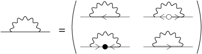
Figure 6: The quark self-energy $\Sigma$ written in the Nambu-Gor’kov basis, cf. Eq. (115). Single straight lines directing to the left/right correspond to $\left([G_{0}^{\mp}]^{-1}+\Sigma^{\mp}\right)^{-1}$. Double straight lines to the left/right correspond to $\mathcal{G}^{\pm}$. Full/empty dots symbolizes the Cooper pair condensate $\Phi^{\pm}$ absorbing/emitting a quasiparticle pair.

In order to proceed one has to make an approximation for $\Gamma_{2}$. We will restrict to two-loop 2PIs. Furthermore, pure gluonic loops are proportional to $T^{2}$ [66] and can be safely neglected in the limit of small temperatures. Consequently, we will consider only the first diagramm in Fig. 5. It is an advantage of the CJT formalism, that truncating $\Gamma_{2}$ will not destroy the self-consistency of the solution. The gluon self-energy is computed as $\Pi=-2\,\delta\Gamma_{2}/\delta\Delta^{T}$, i.e., by cutting a gluon line in the first diagram of Fig. (5). Thus, in our approximation $\Pi$ is simply a quark loop with Nambu-Gor’kov propagators $\mathcal{G}$. Accordingly, the quark self-energy $\Sigma\equiv 2\,\delta\Gamma_{2}/\delta\mathcal{G}^{T}$, is obtained by cutting a quark-line in the same diagram. Its Nambu-Gor’kov structure is shown in Fig. 6. The diagonal components $\Sigma^{\pm}$ correspond to the ordinary self-energies for particles and charge-conjugate particles. The self-energies $\Phi^{\pm}$ symbolize the Cooper pair condensate connecting particles and charge-conjugate particles. In the following, also the term gap matrix will be used for $\Phi^{+}$. Explicitly, the Nambu-Gor’kov components of $\Sigma$ read

$$\Sigma^{+}(K) = -g^{2}\,\frac{T}{V}\sum\limits_{Q}\gamma^{\mu}T_{a}\,\mathcal{G}^{+}(Q)\,\gamma^{\nu}T_{b}\,\Delta_{\mu\nu}^{ab}(K-Q)\,\,,$$ (121)

$$\Sigma^{-}(K) = -g^{2}\,\frac{T}{V}\sum\limits_{Q}\gamma^{\mu}T_{a}^{T}\,\mathcal{G}^{-}(Q)\,\gamma^{\nu}T_{b}^{T}\,\Delta_{\mu\nu}^{ab}(K-Q)\,\,,$$ (122)

$$\Phi^{+}(K) = g^{2}\,\frac{T}{V}\sum\limits_{Q}\gamma^{\mu}T_{a}^{T}\,\Xi^{+}(Q)\,\gamma^{\nu}T_{b}\,\Delta_{\mu\nu}^{ab}(K-Q)\,\,,$$ (123)

$$\Phi^{-}(K) = g^{2}\,\frac{T}{V}\sum\limits_{Q}\gamma^{\mu}T_{a}\,\Xi^{-}(Q)\,\gamma^{\nu}T_{b}^{T}\,\Delta_{\mu\nu}^{ab}(K-Q)\,\,.$$ (124)

Inserting these self-energies (and the corresponding one for the gluons) into the Dyson-Schwinger equations (106) and (107) one obtains a coupled set of integral equations which has to be solved self-consistently. In particular, the Dyson-Schwinger equations for the off-diagonal components $\Phi^{\pm}$ of the inverse propagator $\mathcal{G}^{-1}$, i.e., Eqs. (123) and (124), are the gap equations for the color-superconducting condensate.

Even in the mean-field approximation applied here a completely self-consistent solution of the coupled set of Dyson-Schwinger equations is not feasible. Therefore, we will refrain from determining the gluon propagator self-consistently but resort to its hard-dense loop approximation [66]. Thus we will obtain a well-controlled, approximate solution of the gap-equation as it will be demonstrated in next section.

7 Quasi-particle excitations in color superconductor

In this section we analyse how the presence of a Cooper pair condensate affects the excitation spectrum of quasiparticles. To this end, the poles of the propagator $\mathcal{G}$ have to be determined. The excitation spectrum depends on the specific symmetry broken pattern of the superconducing phase considered here, cf. Sec. 3 and 5. To this end, we first analyse the Dirac, color and flavor structure of the varios terms contained in $\mathcal{G}$, cf. Eq. (119). As we work in the ultra-relativistic limit, $m=0$, we may expand the free (charge conjugate) quark propagator $G_{0}^{\pm}$ in terms of positive and negative energy states using the projection operator $\Lambda_{\mathbf{k}}^{e}\equiv(1+e\,\gamma_{0}\,\bm{\mbox{$\gamma$}}\cdot\widehat{\mathbf{k}})/2$, where $e=+$ projects on (charge conjugate) quarks and $e=-$ projects on (charge conjugate) antiquarks. One obtains for the respective free propagators

$$[G_{0}^{\pm}]^{-1}(K)=\gamma_{0}\sum_{e=\pm}\left[k_{0}-(ek\mp\mu)\right]\,\Lambda_{\mathbf{k}}^{e}\,\,.$$ (125)

Furthermore, $[G_{0}^{\pm}]^{-1}$ is diagonal in color and flavor space. To simplify the further analysis we anticipate that in weak coupling limit adopted here and to subleading order, the regular self-energy $\Sigma^{\pm}$ may be approximated by its one-loop approximation [67, 68, 69] in the leading logarithmic order (cf. Ref. [70] for result beyond the leading logarithmic order). In this approximation, the self-consistent propagators in Eqs. (121,122) are replaced by free propagators. In particular, this amounts to neglecting the Cooper pair condensate in $\Sigma^{\pm}$, so that $\Sigma^{\pm}$ is diagonal in color and flavor space. In Dirac space one finds [67, 68, 69]

$$\Sigma^{+}(K)=\Sigma^{-}(K)\approx\gamma_{0}\;\bar{g}^{2}\left(k_{0}\ln\frac{M^{2}}{k_{0}^{2}}+i\pi|k_{0}|\right)\;,$$ (126)

where $\bar{g}\equiv g/(3\sqrt{2}\pi)$ and $M^{2}\equiv(3\pi/4)m_{g}^{2}$ (with $m_{g}^{2}=N_{f}\frac{g^{2}\mu^{2}}{6\pi^{2}}$). To subleading order it is sufficient to include only the real part of $\Sigma^{\pm}(K)$ [68]. Its effect is simply a shift of the quasiparticle poles, $k_{0}\rightarrow k_{0}/Z(k_{0})$, where we introduced the quark wave function renormalization function

$$Z(k_{0})\equiv\left(1+\bar{g}^{2}\ln\frac{M^{2}}{k_{0}^{2}}\right)^{-1}\;.$$ (127)

The imaginary part of $\Sigma^{\pm}(K)$ can be shown to contribute beyond subleading order [71] and therefore will be neglected in the following. Physically, the imaginary part of $\Sigma^{\pm}(K)$ gives rise to a finite life-time of the quasi-particles off the Fermi surface, which reduces the magnitude of the gap at sub-subleading order [71].

Turning to the structure of $\Phi^{\pm}$ we introduce a compact notation following [30],

$$\Phi^{+}(K)=\sum_{e=\pm}\phi^{e}(K)\,\mathcal{M}_{\mathbf{k}}\,\Lambda_{\mathbf{k}}^{e}\,\,,$$ (128)

where $\phi^{e}$, the so-called gap function, is a scalar function of 4-momentum $K$. In general, the quantity $\mathcal{M}_{\mathbf{k}}$ is a matrix in color, flavor, and Dirac space, which is determined by the symmetries of the color-superconducting order parameter. It can be chosen such that

$$[\mathcal{M}_{\mathbf{k}},\Lambda_{\mathbf{k}}^{e}]=0\;.$$ (129)

Note that the above is only valid in massless case. For the spin-0 phases 2SC and CFL the strucure of $\mathcal{M}_{\mathbf{k}}$ has been determined in Sec. 5. In Tab. 6 the corresponding structures for three spin-1 phases, the CSL, the polar and the A-phase, are shown. Note that these spin-1 phases are actually the mixtures of longitudinal and transverse phases, and that the transverse phases have the largest gaps.

Table 6: The structure of the matrices $\mathcal{M}_{\mathbf{k}}$ in various color-superconducting phases. The last two columns show the two eigenvalues $\lambda_{r}$ of $L_{\mathbf{k}}$ and their degeneracy $d_{r}$ (counting color-flavor degrees of freedom in the 2SC and CFL phases, and color-Dirac degrees of freedom in the three spin-one phases).

phase	${\cal M}_{\bf k}$	$\lambda_{1}\;(d_{1})$	$\lambda_{2}\;(d_{2})$
2SC	$\gamma_{5}\,\sigma_{2}\,J_{3}$	1 (4)	0 (2)
CFL	$\gamma_{5}\,{\bf I}\cdot{\bf J}$	4 (8)	1 (1)
CSL	${\bf J}\cdot\left[\hat{\bf k}+\mbox{\boldmath$\gamma$}_{\perp}({\bf k})\right]$	4 (4)	1 (8)
polar	$J^{3}\left[\hat{k}^{z}+\gamma^{z}_{\perp}({\bf k})\right]$	1 (8)	0 (4)
A	$J^{3}\left[\hat{k}^{x}+i\hat{k}^{y}+\gamma^{x}_{\perp}({\bf k})+i\gamma^{y}_{\perp}({\bf k})\right]$	2 (4)	0 (8)

With representation (128) for $\Phi^{+}$ one may rewrite the second term on the r.h.s. of Eq. (119)

$$\Phi^{-}G^{-}\Phi^{+}[G^{-}]^{-1}=\sum_{e=\pm}|\phi^{e}(K)|^{2}L_{\mathbf{k}}\Lambda_{\mathbf{k}}^{-e},$$

where we introduced

$$L_{\mathbf{k}}\equiv\gamma_{0}\mathcal{M}_{\mathbf{k}}^{\dagger}\mathcal{M}_{\mathbf{k}}\gamma_{0}\;.$$ (130)

Since $L_{\mathbf{k}}$ is hermitian, it has real eigenvalues, $\lambda_{r}$, and can be expanded in terms of a complete set of orthogonal projectors, $\mathcal{P}_{\mathbf{k}}^{r}$,

$$L_{\mathbf{k}}=\sum_{r}\lambda_{r}\mathcal{P}_{\mathbf{k}}^{r}\,\,.$$ (131)

In the five phases considered here, there are only two distinct eigenvalues and therefore two distinct projectors. The eigenvalues are also listed in Tab. 6, and the projectors can be expressed in terms of $L_{\mathbf{k}}$ via

$$\mathcal{P}_{\mathbf{k}}^{1,2}=\frac{L_{\mathbf{k}}-\lambda_{2,1}}{\lambda_{1,2}-\lambda_{2,1}}\,\,.$$ (132)

Note, that $[L_{\mathbf{k}},\Lambda_{\mathbf{k}}^{e}]=[\mathcal{P}_{\mathbf{k}}^{1,2},\Lambda_{\mathbf{k}}^{e}]=0$. Since the projectors $\mathcal{P}^{r}\,\Lambda_{\mathbf{k}}^{e}$ form a basis in color, flavor, and Dirac space, inverting the term in the curly brackets in Eq. (119) is straightforward, yielding

$$\mathcal{G}^{+}(K)=[G^{-}]^{-1}(K)\sum_{e,r}\mathcal{P}_{\mathbf{k}}^{r}\,\Lambda_{\mathbf{k}}^{-e}\,\frac{1}{[k_{0}/Z(k_{0})]^{2}-\left[\epsilon_{\mathbf{k},r}^{e}(\phi^{e})\right]^{2}}\,\,,$$ (133)

where

$$\epsilon_{\mathbf{k},r}^{e}(\phi^{e})=\left[(ek-\mu)^{2}+\lambda_{r}\,|\phi^{e}|^{2}\right]^{1/2}\,\,.$$ (134)

Inserting Eqs. (128,133) into Eq. (120) yields

$$\Xi^{+}(K)=-\sum_{e,r}\gamma_{0}\,\mathcal{M}_{\mathbf{k}}\,\gamma_{0}\,\mathcal{P}_{\mathbf{k}}^{r}\,\Lambda_{\mathbf{k}}^{-e}\,\frac{\phi^{e}(K)}{[k_{0}/Z(k_{0})]^{2}-\left[\epsilon_{\mathbf{k},r}^{e}(\phi^{e})\right]^{2}}\,\,.$$ (135)

Obviously, the poles of the propagators $\mathcal{G}^{+}$ and $\Xi^{+}$ are located at $k_{0}\equiv\pm Z(k_{0})\,\epsilon_{\mathbf{k},r}^{e}(\phi^{e})$ and the same result can be obtained for the propagators $\mathcal{G}^{-}$ and $\Xi^{-}$. Eq. (134) is the relativistic analogue of the standard BCS dispersion relation. The presence of the Cooper pair condenstate has generated a gap in the excitation spectrum of quasiquarks, $e=+$. Hence, even on the Fermi surface, $k=\mu$, they carry a non-zero amount of energy, which is of the order of the gap function, $\epsilon_{\mu,r}^{+}=\sqrt{\lambda_{r}}\,\phi^{+}$. To excite (generate) a pair of a quasiparticle and a quasiparticle hole therefore costs at least the energy $2\sqrt{\lambda_{r}}\,\phi^{+}$. Such an excitation process can be interpreted as a break-up of a Cooper pair and the required energy as the Cooper pair binding energy. To investigate which quasiparticles exhibit a gap in their excitation spectrum one has to determine the eigenvalues $\lambda_{r}$ of the operator $L_{\mathbf{k}}$. For the phases considered here, $L_{\mathbf{k}}$ has one or two non-zero eigenvalues. For $\lambda_{r}=0$ the respective quasi-particles remain ungapped. The degeneracy $d_{r}$ gives the number of excitation branches with the same gap, $\sqrt{\lambda_{r}}\,\phi^{+}$.

Finally, for quasi anti-quarks, $e=-$, the dispersion relation hardly differs from the non-interacting case in the limit of large $\mu$, $\epsilon_{\mathbf{k}}^{-}\approx k+\mu$.

In the next section, the gap equation (123) for the gap function $\phi^{e}(K)$ will be solved for quasi-particle excitations, $e=+$, at zero temperature in order to determine the magnitude of the gap in their excitation spectrum.

8 Solving the gap equation

To obtain the Dyson-Schwinger equation for the scalar gap function $\phi^{+}(K)$ one inserts Eq. (135) into Eq. (123), multiplies from the right with $\mathcal{M}_{\mathbf{k}}^{\dagger}\Lambda_{\mathbf{k}}^{+}$, and traces over color, flavor, and Dirac space. The result is the so-called gap equation

$$\phi^{+}(K) = g^{2}\,T\sum_{n}\int\frac{d^{3}\mathbf{q}}{(2\pi)^{3}}\sum_{e^{\prime},s}\frac{\phi^{e^{\prime}}(Q)}{\left[q_{0}/Z(q_{0})\right]^{2}-\left[\epsilon_{\mathbf{q},s}^{e^{\prime}}(\phi^{e^{\prime}})\right]^{2}}$$ (136)

$$\times\Delta_{\mu\nu}^{ab}(K-Q)\mathcal{T}_{ab,s}^{\mu\nu,ee^{\prime}}(\mathbf{k},\mathbf{q})\,\,,$$

where

$$\mathcal{T}_{ab,s}^{\mu\nu,ee^{\prime}}(\mathbf{k},\mathbf{q})\equiv-\frac{\mathrm{Tr}\left[\gamma^{\mu}T_{a}^{T}\gamma_{0}\mathcal{M}_{\mathbf{q}}\gamma_{0}\mathcal{P}_{\mathbf{q}}^{s}\Lambda_{\mathbf{q}}^{-e^{\prime}}\gamma^{\nu}T_{b}\mathcal{M}_{\mathbf{k}}^{\dagger}\Lambda_{\mathbf{k}}^{e}\right]}{\mathrm{Tr}\left[\mathcal{M}_{\mathbf{k}}\mathcal{M}_{\mathbf{k}}^{\dagger}\Lambda_{\mathbf{k}}^{e}\right]}\,\,.$$ (137)

The power counting scheme for the various contributions arising on the r.h.s. of the gap equation (136) is the same for all phases considered here. Due to the factor $g^{2}$ the integral must give terms proportional to $\phi/g^{2}$ in order to fulflill the equality. They contribute to the gap function at the largest possible order, $O(\phi)$, and are therefore referred to as leading order contributions. Terms of order $\phi/g$ from the integral contribute at the order $O(g\phi)$ to the gap function and are called subleading order corrections. Sub-subleading order corrections contributing at $O(g^{2}\phi)$ to the gap function have not been calculated yet and will be neglected in the following.

In principle it is possible to proceed without deciding on one of the specific phases considered here. However, to keep the calculation as transparent as possible we restrict to the 2SC phase. The results for the other phases will be summarized at the end of this section.

As already mentioned in the previous section, the Dyson-Schwinger equation for the gluon propagator will not be solved self-consistently. Instead we will adopt the gluon propagator in its HDL approximation. In pure Coulomb gauge they can be decomposed into a electric (or longitudinal) and a magnetic (or transversal) part as [5, 66]

$$\Delta_{00}(P) = \Delta_{\ell}(P)$$

$$\Delta_{0i}(P) = 0$$

$$\Delta_{ij}(P) = \Delta_{t}(P)\left(\delta_{ij}-\hat{p}_{i}\hat{p}_{j}\right)\,\,.$$

with $P\equiv K-Q$ and the longitudinal and transverse propagators $\Delta_{\ell,t}$. Since the HDL propagators are diagonal in adjoint color space, $\Delta_{ab}^{\mu\nu}=\delta_{ab}\Delta^{\mu\nu}$, the color indices can safely be suppressed. The explicit forms of the propagators $\Delta_{\ell,t}$ can be found in Ref. [5, 66]. For our purposes the approximative forms of $\Delta_{\ell,t}$ given below are sufficient. As will be substantiated in the following the leading order contribution to the gap arises from almost static magnetic gluons with

$$\Delta_{t}^{\mathrm{LDM}}(P)\simeq\frac{p^{4}}{p^{6}+M^{4}\,\omega^{2}}\Theta(M-p).$$ (138)

The term $M^{4}\omega^{2}$ arises from Landau-damping which dynamically screens magnetic gluons at the scale $p\sim M^{2/3}\omega^{1/3}$. Consequently almosr static magnetic gluons dominate the interaction between quarks at large distances. Subleading order corrections come from non-static magnetic gluons with

$$\Delta_{t}^{\mathrm{NSM}}(p)\simeq\frac{1}{p^{2}}\Theta(p-M)\,\,,$$ (139)

and from static electric gluons with

$$\Delta_{\ell}^{\mathrm{SE}}(p)\simeq-\frac{1}{p^{2}+3m_{g}^{2}}\,\,,$$ (140)

where the constant mass term $m_{g}^{2}=N_{f}\frac{g^{2}\mu^{2}}{6\pi^{2}}$ provides Debye-screening at the scale $p\sim g\mu$. As the gap equation (136) requires a self-consistent solution, we may proceed by first giving the known result and confirming it in the following. At zero temperature the 2SC gap function assumes for on-shell quasiparticles ($e=+$) with momenta $k\approx\mu$ the value

$$\phi_{0}^{\mathrm{2SC}}=2\tilde{b}b_{0}^{\prime}\mu\exp\left(-\frac{\pi}{2\bar{g}}\right)\,\,,$$ (141)

where

$$\tilde{b} \equiv 256\pi^{4}\left(\frac{2}{N_{f}g^{2}}\right)^{5/2}$$

$$b_{0}^{\prime} \equiv \exp\left(-\frac{\pi^{2}+4}{8}\right)\,\,.$$ (142)

The term in the exponent of Eq. (141) was first determined by Son [72] via a renormalization group analysis taking into account the long-range nature of almost static, Landau-damped magnetic gluons, cf. Eq. (138). Before that, a non-zero magnetic mass (analogous to the Debye-mass for electric gluons) was assumed leading to the standard BCS exponent, $\exp\left(-\frac{3\pi^{2}\Lambda^{2}}{2\mu^{2}g^{2}}\right)$, where $\Lambda^{2}$ is the the typical momentum of the exchanged gluon and $g^{2}/3$ the effective coupling in the anti-triplet channel. This finding was crucial since in the correct exponential (141) the parametric suppression becomes much weaker for small values of $g$, i.e. for large values of $\mu$. The factor $\tilde{b}$ in front of the exponential is generated by the exchange of non-static magnetic (139) and static electric (140) gluons [28, 73, 74]. The prefactor $b_{0}^{\prime}$ is due to the real part of the quark self-energy as given by Eq. (127) [67, 68].

From Tab. (6) we read off

$$\mathcal{M}_{\mathbf{k}} = \gamma_{5}\sigma_{2}J_{3}$$

and hence with Eqs. (130,132) one finds the projectors $\mathcal{P}_{\mathbf{k}}^{1,2}$ to be

$$\mathcal{P}_{\mathbf{k}}^{1} = J_{3}^{2}\;,$$

$$\mathcal{P}_{\mathbf{k}}^{2} = 1-J_{3}^{3}\;,$$

with the eigenvalues $\lambda_{1}=1$ (4-fold) and $\lambda_{2}=0$ (2-fold). This yields

$$\mathcal{T}_{1}^{\ell,ee^{\prime}}(\mathbf{k},\mathbf{q}) = \frac{1}{3}\,\left(1+ee^{\prime}\hat{\mathbf{k}}\cdot\hat{\mathbf{q}}\right)\,\,,$$

$$\mathcal{T}_{1}^{t,ee^{\prime}}(\mathbf{k},\mathbf{q}) = \frac{1}{3}\,\left[3-ee^{\prime}\hat{\mathbf{k}}\cdot\hat{\mathbf{q}}\right.\,\,.$$ (143)

$$\left.-\frac{(ek-e^{\prime}q)^{2}}{p^{2}}\left(1+ee^{\prime}\hat{\mathbf{k}}\cdot\hat{\mathbf{q}}\right)\right]\,\,.$$

and $\mathcal{T}_{2}^{\mu\nu,ee^{\prime}}(\mathbf{k},\mathbf{q})\equiv 0$. Hence, the gapless quasi-particles corresponding to $\mathcal{P}_{\mathbf{k}}^{2}$ do not enter the gap equation. Performing the Matsubara sum in Eq. (136) one then obtains for the gapped branch with the projector $\mathcal{P}_{\mathbf{k}}^{1}$ to subleading order

$$\phi^{+}(\epsilon_{\mathbf{k}}^{e},k) = \frac{g^{2}}{16\pi^{2}k}\int_{\mu-\delta}^{\mu+\delta}dq\,q\sum_{e^{\prime}}Z(\epsilon_{\mathbf{q}}^{e^{\prime}})\,\frac{\phi^{e^{\prime}}(\epsilon_{\mathbf{q}}^{e^{\prime}},q)}{\epsilon_{\mathbf{q}}^{e^{\prime}}}$$ (144)

$$\times\tanh\left(\frac{\epsilon_{\mathbf{q}}^{e^{\prime}}}{2T}\right)\sum\limits_{m=0}^{1}\int_{|k-q|}^{k+q}dp\,p\left(\frac{p^{2}}{kq}\right)^{m}$$

$$\left\{-2\,\Delta_{00}^{\mathrm{SE}}(p)\,\eta_{2m}^{\ell}+\left[\;2\,\Delta_{t}^{\mathrm{NSM}}(p)\right.\right.$$

$$+\Delta_{t}^{\mathrm{LDM}}\left(\epsilon_{\mathbf{q}}^{e^{\prime}}+\epsilon_{\mathbf{k}}^{e},p\right)$$

$$\left.\left.+\Delta_{t}^{\mathrm{LDM}}\left(\epsilon_{\mathbf{q}}^{e^{\prime}}-\epsilon_{\mathbf{k}}^{e},p\right)\right]\eta_{2m}^{t}\right\}.$$

To subleading order the coefficients $\eta_{2m}^{\ell,t}$ are given by $\eta_{0}^{\ell}=\eta_{0}^{t}=2/3$ and $\eta_{2}^{\ell}=-\eta_{2}^{t}=-1/6\,$. (Other phases than 2SC have different coefficients $\eta_{2m}^{\ell,t}$ and possibly have an additional excitation branch. To subleading order, however, the coefficients $\eta_{2m}^{\ell,t}$ (with $-1\leq m\leq 2$) become simple numbers of order $O(1)$ for all phases considered here. It follows that the values of the respective gap functions differ only at subleading order [30].) To obtain Eq. (144) several sub-subleading contributions are dropped. For example, the integration over $q$ can be confined to a narrow interval of length $2\delta$ around the Fermi surface, $\delta\sim g\mu$, since the gap function peaks strongly around the Fermi surface. Furthermore, use was made of the fact, that the gap function must be an even function in $K$, $\phi^{e}(K)=\phi^{e}(-K)$. This property follows from the antisymmetry of the fermionic quark wave-functions. One has with $\psi_{C}(K)=C\bar{\psi}^{T}(-K)$, $\bar{\psi}_{C}(K)=\psi^{T}(-K)C$ and $C=-C^{-1}=-C^{T}$

$$\sum\limits_{K}\bar{\psi}_{C}(K)\Phi^{+}(K)\psi(K) \equiv -\sum\limits_{K}\psi^{T}(K)\left[\Phi^{+}(K)\right]^{T}\bar{\psi}_{C}^{T}(K)$$

$$= \sum\limits_{K}\bar{\psi}_{C}(K)C^{-1}\left[\Phi^{+}(-K)\right]^{T}C\psi(K)\;.$$

Hence, the gap matrix must fulfill

$$C\Phi^{+}(K)C^{-1} = \left[\Phi^{+}(-K)\right]^{T}.$$

Since in the 2SC case we have $C\gamma_{5}\Lambda_{\mathbf{k}}^{e}C^{-1}=[\gamma_{5}\Lambda_{-\mathbf{k}}^{e}]^{T}$ and $[J_{3}\tau_{2}]^{T}=J_{3}\tau_{2}$, it follows that $\phi^{e}(K)=\phi^{e}(-K)$. Moreover, the gap function was assumed to be isotropic in momentum space, $\phi^{e}(\mathbf{k})\equiv\phi^{e}(k)$ [30]. Finally, all imaginary contributions arising from the energy dependence of the gluon propagators and the gap function itself are neglected. It follows, that the energy dependence of the gap function occuring in the final result has not been determined self-consistently. In Ref. [73] it is argued that imaginary contributions are negligible to subleading order.

Using the well-known solution Eq. (141) for the 2SC gap function it is now straightforward to confirm that the various gluon sectors occuring in Eq. (144) indeed contribute at the claimed orders of magnitude. For the static electric and the non-static magnetic gluons the integral over $q$ gives for $e^{\prime}=+$ and $m=1$

$$g^{2}\phi^{+}\int_{\mu-\delta}^{\mu+\delta}\frac{dq}{\epsilon_{\mathbf{q}}^{+}} = 2g^{2}\phi^{+}\ln\left(\frac{\delta+\sqrt{\delta^{2}+(\phi^{+})^{2}}}{\phi^{+}}\right)$$ (145)

$$\simeq 2g^{2}\phi^{+}\ln\left(\frac{2\,\delta}{\phi^{+}}\right)$$

$$\sim g^{2}\phi^{+}\ln\left[\frac{g}{\exp(-1/g)}\right]\sim g\phi^{+},$$

where for simplicity the gap function is moved out of the integral and the fact was used that $\delta\sim g\mu\gg\phi^{+}\sim\mu\exp(-1/g)$. Note that this result does not depend on the specific choice of $\delta$, as long as $\delta$ is of the order $\delta\sim g^{c}(\mu^{a}\phi^{b})^{\frac{1}{a+b}}$ with some numbers $a\neq 0$ and $b,c$. The integral over $p$ in combination with the factor $1/k\sim\mu$ is of order $O(1)$. It follows that static electric and non-static magnetic gluons actually contribute at subleading order to the gap function. The above integral and the logarithm that follows from it also appear in normal BCS theory [75]. Therefore we will refer to it as the BCS-logarithm. For $e^{\prime}=-$, one has $\epsilon_{\mathbf{q}}^{-}\simeq q+\mu$ and the contribution corresponding to Eq. (145) is of order $g^{2}\phi\delta/\mu\sim g^{3}\phi$, i.e. beyond subleading order.

In the case of almost static, Landau-damped magnetic gluons the integration over $q$ can be estimated as in Eq. (145). Choosing the term with $e^{\prime}=+$ and $m=0$ and canceling $q\simeq\mu$ in the integral with the factor $1/k\sim 1/\mu$ at the front one obtains the BCS-logarithm. In order to render the total contribution of leading order, the $p-$integral must yield an additional factor $1/g$. Using the notation $\omega_{\pm}\equiv\epsilon_{\mathbf{q}}^{+}\pm\epsilon_{\mathbf{k}}^{+}$ one finds as the dominant contribution the term

$$\int_{k-q}^{M}dp\frac{p^{5}}{p^{6}+M^{4}\omega_{\pm}^{2}} = \frac{1}{6}\ln\left[\frac{M^{6}+M^{4}\omega_{\pm}^{2}}{(k-q)^{6}+M^{4}\omega_{\pm}^{2}}\right]$$ (146)

$$\sim \ln\left(\frac{M^{2}}{\omega_{\pm}^{2}}\right)\sim\frac{1}{g}\,\,.$$

The last two steps are justified if one chooses for the cut-off $\delta$ in the $q$ integral $\delta=(M^{2}\phi)^{1/3}$. Consequently, in combination with the BCS-logarithm (145) this indeed is a leading order contribution.

After having identified the leading and subleading order contributions, one evaluates the $p$ integral in Eq. (144) and finds to subleading order (supressing all the superscripts $e=e^{\prime}=+$)

$$\phi(\epsilon_{\mathbf{k}},k) = \bar{g}^{2}\int_{0}^{\delta}d(q-\mu)Z(\epsilon_{\mathbf{q}})\frac{\phi(\epsilon_{\mathbf{q}},q)}{\epsilon_{\mathbf{q}}}$$ (147)

$$\times\tanh\left(\frac{\epsilon_{\mathbf{q}}}{2T}\right)\frac{1}{2}\ln\left(\frac{b^{2}\mu^{2}}{|\epsilon_{\mathbf{q}}^{2}-\epsilon_{\mathbf{k}}^{2}|}\right)\,\,.$$

How to solve Eq. (147) to subleading order is demonstrated explicitly in [68]. In the following, only some important steps are presented. As first proposed by Son [72] one approximates

$$\frac{1}{2}\ln\left(\frac{b^{2}\mu^{2}}{|\epsilon_{\mathbf{q},s}^{2}-\epsilon_{\mathbf{k},r}^{2}|}\right) \simeq \Theta(\epsilon_{\mathbf{q},s}-\epsilon_{\mathbf{k},r})\ln\left(\frac{b\mu}{\epsilon_{\mathbf{q},s}}\right)$$

$$+\Theta(\epsilon_{\mathbf{k},r}-\epsilon_{\mathbf{q},s})\ln\left(\frac{b\mu}{\epsilon_{\mathbf{k},r}}\right)\,\,.$$

Rewriting Eq. (147) in terms of the new variables [68]

$$x \equiv \bar{g}\ln\left(\frac{2b\mu}{k-\mu+\epsilon_{k}}\right),$$

$$y \equiv \bar{g}\ln\left(\frac{2b\mu}{q-\mu+\epsilon_{q}}\right)$$ (148)

and differentiating twice with respect to $x$ one can transform the gap equation into the form of Airy’s differential equation. Its solution can be written as

$$\phi(x)\equiv\phi_{0}^{\mathrm{2SC}}F(x)\,\,,$$ (149)

where $\phi_{0}^{\mathrm{2SC}}$ is given by Eq. (141) and $F(x)$ is a combination of different Airy-functions [68]. The situation simplifies considerably when one neglects the effect of the normal quark self-energy, i.e. the factor $Z(\epsilon_{\mathbf{q}})$ in Eq. (147). Besides $b_{0}^{\prime}\equiv 1$ in Eq. (142), one then finds $F(x)\equiv\sin x$ [72, 73], as the differential equation for $\phi$ simplifies to that of an harmonic oszillator. For $|k-\mu|\sim\phi$ one obtains $x=\pi/2+O(\bar{g})$, while for $|k-\mu|\sim g\mu$ it is $x\sim O(\bar{g})$. Hence, for momenta exponentially close to the Fermi surface, $|k-\mu|\sim\phi$, the on-shell gap function is $\phi(\epsilon_{k},k)=\phi_{0}^{\mathrm{2SC}}[1+O(\bar{g}^{2})]$, i.e. constant to subleading order. Otherwise, for example for momenta $|k-\mu|\sim g\mu$, one has already $\phi(\epsilon_{k},k)=\bar{g}\phi_{0}^{\mathrm{2SC}}$. Hence, the on-shell gap-function is sharply peaked around the Fermi surface.

The gap for on-shell quasi-particles at the Fermi surface in the 2SC phase as given by Eq. (141) is valid for asymptotic densities where $g(\mu)\ll 1$. At chemical potentials of physical relevance, however, one has $g(\mu)\sim O(1)$. Then sub-subleading terms which are corrections of order $O(g)$ to the prefactor of the gap function in principle have to be accounted for. So far, they have not been calculated. Keeping this caveat in mind, it is still instructive to extrapolate the present result down to physical quark-chemical potentials of several hundred MeV. As explained in more detail in Ref. [5] one finds $\phi_{0}^{\mathrm{2SC}}\simeq 10$ MeV.

As already mentioned before, the solution of the gap equation in all phases considered here [30, 34] can be written in a general form. For all considered phases it is found that differences arises only in the prefactor in front of the exponential, i.e. are only of subleading order [30, 34]:

$$\phi_{0}=2\tilde{b}b^{\prime}_{0}\mu e^{-d}e^{-\varsigma}\exp\left(-\frac{\pi}{2\bar{g}}\right),$$ (150)

where $d=0$ and $\varsigma=\ln(\langle\lambda_{1}\rangle^{a_{1}}\langle\lambda_{2}\rangle^{a_{2}})^{1/2}$ for all spin-zero phases. Here the coefficients $a_{1},a_{2}$ are positive constants obeying $a_{1}+a_{2}=1$. In spin-one phases $d\neq 0$ and $\varsigma$ are given by

$$\varsigma = \frac{1}{2}\frac{\left\langle n_{1}\lambda_{q,1}\ln\lambda_{q,1}+n_{2}\lambda_{q,2}\ln\lambda_{q,2}\right\rangle_{\mathbf{\widehat{q}}}}{\left\langle n_{1}\lambda_{q,1}+n_{2}\lambda_{q,2}\right\rangle_{\mathbf{\widehat{q}}}}$$

where $n_{r}$ is the degeneracy factor for the excitation branch. Generally the eigenvalues $\lambda_{r}$ depend on the direction of the quark momentum, so the angular average $\langle\rangle$ is taken for all directions $\mathbf{\widehat{q}}$. For all spin-one phases considered in this paper, $d$ is about $5$, it means $e^{-d}\sim 10^{-2}-10^{-3}$, which strongly reduce spin-one gaps relative to spin-zero-gaps. Tab. (7) give an overview of the gaps of the different phases in units of the 2SC gap, $\phi_{0}^{\mathrm{2SC}}$.

Table 7: The value of the gap function at the Fermi surface, $\phi_{0}$ in units of its value in the 2SC phase, and the critical temperature, in units of its value expected from BCS theory, and in units of the critical temperature in the 2SC phase, $T_{c}^{\mathrm{2SC}}$.

phase	$d$	$\phi_{0}/\phi_{0}^{{\rm 2SC}}$	$T_{c}/T_{c}^{{\rm BCS}}$	$T_{c}/T_{c}^{{\rm 2SC}}$
2SC	0	1	1	1
CFL	0	$2^{-1/3}$	$2^{1/3}$	1
CSL	5	$2^{-1/6}\,e^{-d}$	$2^{1/6}$	$e^{-d}$
polar	5	$e^{-d}$	$1$	$e^{-d}$
A	21/4	$e^{-d}$	$1$	$e^{-d}$

Tab. (7) also lists the critical temperatures $T_{c}$ for all considered phases [30, 34, 68, 73]. Generally the ratio of the critical temperatures to the zero temperature gaps on the Fermi surface is given by

$$\frac{T_{c}}{\phi_{0}} = \frac{e^{\gamma}}{\pi}e^{-\varsigma}\simeq 0.57e^{-\varsigma}$$ (151)

where $\gamma\simeq 0.577$ is the Euler-Mascheroni constant. An important feature is that in such single-gapped phases as the 2SC, polar or A phase, the ratio is the same as in BCS theory (the so-called BCS ratio $T_{c}/\phi_{0}=0.57$) [73]. For phases with more than two different excitations, such as the CFL or CSL phase, one has $e^{-\varsigma}\neq 1$, which violats the BCS ratio [29, 30], cf. the third column in Tab. (7). Another situation where the BCS ratio is violated is that the gap is anisotropic in momentum direction. Expressing the respective critical temperatures $T_{c}$ in terms of $T_{c}^{\mathrm{2SC}}$ the factor $e^{-\varsigma}$ in Eq. (150) cancels the factor $e^{-\varsigma}$ in Eq. (151) yielding $T_{c}/T_{c}^{\mathrm{2SC}}=e^{-d}$, which is listed in the forth column of Tab. (7). The transition temperature of a superconducting phase is normally regarded as the temperature where the gap disappears in the gap equation. This is justified in the mean field approximation. If one goes beyond the mean field approximation by including the fluctuation of the diquark fields, even above the transition temperature the ’gap’ (the so-called pseudogap) is not vanishing [76, 77]. The transition temperature can also be modified by the gluon fluctuation which is beyond the mean field approximation [78].

We know that in the gap equation there are gluon propagators. If one changes the gauge parameter of the gluon propagator, the question arises if the gap would be invariant. The answer is yes under the following conditions [64]: (a) the gap equation is put on the mass-shell, and (b) the poles of the gluon propagator do not overlap with those of the quark propagator. However in the mean field approximation the gap depends on the gauge parameter at the sub-subleading level if one imposes the on-shell condition [79, 80].

In intermediate coupling regime, the superconducting phases can be investigated within a Dyson-Schwinger approach for the quark propagator in QCD [81, 82]. It was found that at moderate chemical potentials the quasiparticle pairing gaps are several times larger than the extrapolated weak-coupling results.

9 Debye and Meissner masses

In this section we will address another two important energy scales in superconductivity: Debye and Meissner masses. The Debye mass for gluons/ photons characterizes the screening of the chromoelectric/electric charge in the medium, while the Meissner mass leads to expelling the chromomagnetic/magnetic field out of the type-I color/normal superconductor. We consider the weak coupling limit where the gap is parametrically smaller than the Debye or Meissner mass, so the coherence length (inverse of the gap) is much larger than the penetration length (inverse of the Meissner mass), which means in the weak coupling limit, all color superconductors are of type-I.

The Debye and Meissner masses for gluons or photons can be calculated through gluon or photon polarization tensors and taking the static limit ($p_{0}=0$, $\mathbf{p}\rightarrow 0$). The polarization tensors depend on the diquark condensate through the quark propagators in the quark loop. The self-energies with full momentum dependence and the spectral densities of longitudinal and transverse gluons at zero temperature in color-superconducting quark matter was studied in detail in [83, 84, 85]. In some color superconducting phases the $U(1)$ charge which can propagate in the medium is the rotated or new photon. It can be found by symmetry analysis shown in previous section or by diagonalizing polarization tensors for both the photon and gluons. We can treat the photon in the same footing as eight gluons by enlarging gluon’s color indices to denote the photon by $a=0$. Diagonalizing the polarization tenors with respect to new ’color’ indices $a=0,1-8$, we can find Deybe and Meissner masses of the rotated photon and gluon which are eigenvalues of the resulting mass matrices. The detail calculation is carried out in Ref. [86]. The results are listed in Tab. (8-10).

Table 8: Zero-temperature Debye masses. All masses are given in units of $N_{f}\mu^{2}/(6\pi^{2})$, where $N_{f}=2$ in the 2SC phase, $N_{f}=3$ in the CFL phase, and $N_{f}=1$ in the polar and CSL phases. We use the abbreviations $\zeta\equiv(21-8\ln 2)/54$, $\alpha\equiv(3+4\ln 2)/27$, and $\beta\equiv(6-4\ln 2)/9$.

	$m_{D,aa}^{2}$								$m_{D,a\gamma}^{2}=m_{D,\gamma a}^{2}$		$m_{D,\gamma\gamma}^{2}$
a	1	2	3	4	5	6	7	8	1-7	8	0
2SC	0			$3g^{2}/2$				$3g^{2}$	0	0	$2e^{2}$
CFL	$3\zeta g^{2}$								0	$-2\sqrt{3}\zeta eg$	$4\zeta e^{2}$
polar	0			$3g^{2}/2$				$3g^{2}$	0	0	$18q^{2}e^{2}$
CSL	$3\beta g^{2}$	$3\alpha g^{2}$	$3\beta g^{2}$	$3\beta g^{2}$	$3\alpha g^{2}$	$3\beta g^{2}$	$3\alpha g^{2}$	$3\beta g^{2}$	0	0	$18q^{2}e^{2}$

Table 9: Zero-temperature Meissner masses. All results are given in the same units as the Debye masses in Table 8. The abbreviations of Table 8 are used.

	$m_{M,aa}^{2}$								$m_{M,a\gamma}^{2}=m_{M,\gamma a}^{2}$		$m_{M,\gamma\gamma}^{2}$
a	1	2	3	4	5	6	7	8	1-7	8	0
2SC	0			$g^{2}/2$				$g^{2}/3$	0	$eg/(3\sqrt{3})$	$e^{2}/9$
CFL	$\zeta g^{2}$								0	$-2\zeta eg/\sqrt{3}$	$4\zeta e^{2}/3$
polar	0			$g^{2}/2$				$g^{2}/3$	0	$2qeg/\sqrt{3}$	$4q^{2}e^{2}$
CSL	$\beta g^{2}$	$\alpha g^{2}$	$\beta g^{2}$	$\beta g^{2}$	$\alpha g^{2}$	$\beta g^{2}$	$\alpha g^{2}$	$\beta g^{2}$	0	0	$3q^{2}e^{2}$

We distinguish between the normal-conducting and the superconducting phase. In the normal-conducting phase, i.e. for temperatures larger than the critical temperature for the superconducting phase transition, $T\geq T_{c}$, Meissner mass is vanishing , i.e., as expected, there is no Meissner effect in the normal-conducting state. However, there is electric screening for temperatures larger than $T_{c}$. Here, the Debye mass solely depends on the number of quark flavors and their electric charge. We find for $T\geq T_{c}$ (with $a=1,\cdots,8$)

$$m_{D,aa}^{2} = 3N_{f}\frac{g^{2}\mu^{2}}{6\pi^{2}}$$

$$m_{D,a\gamma}^{2} = 0$$

$$m_{D,\gamma\gamma}^{2} = 18\sum_{n}q_{n}^{2}\frac{e^{2}\mu_{n}^{2}}{6\pi^{2}}.$$

where $q_{n}$ is the electric charge for the quark flavor labled by $n$. Consequently, the $9\times 9$ Debye mass matrix is already diagonal. Electric gluons and electric photons are screened.

The masses in the superconducting phases are more interesting. The results for all phases are collected in Tab. (8) (Debye masses) and Tab. (9) (Meissner masses). The physically relevant, or “rotated”, masses are obtained after a diagonalization of the $9\times 9$ mass matrices. We see from these tables that all off-diagonal gluon masses, $a,b=1-8$, as well as all mixed masses for $a=1-7$ vanish. Furthermore, in all cases where the mass matrix is not diagonal, we find $m_{8\gamma}^{2}=m_{88}m_{\gamma\gamma}$. We collect the rotated masses and mixing angles for all phases in Tab. (10).

Table 10: Zero-temperature rotated Debye and Meissner masses in units of $N_{f}\mu^{2}/(6\pi^{2})$ and mixing angles for electric and magnetic gauge bosons. The constants $\zeta$, $\alpha$, and $\beta$ are defined as in Tables 8 and 9.

	$\tilde{m}_{D,88}^{2}$	$\tilde{m}_{D,\gamma\gamma}^{2}$	$\cos^{2}\theta_{D}$	$\tilde{m}_{M,88}^{2}$	$\tilde{m}_{M,\gamma\gamma}^{2}$	$\cos^{2}\theta_{M}$
2SC	$3\,g^{2}$	$2\,e^{2}$	1	$\frac{1}{3}g^{2}+\frac{1}{9}e^{2}$	0	$3g^{2}/(3g^{2}+e^{2})$
CFL	$(4e^{2}+3g^{2})\zeta$	0	$3g^{2}/(3g^{2}+4e^{2})$	$\left(\frac{4}{3}e^{2}+g^{2}\right)\zeta$	0	$3g^{2}/(3g^{2}+4e^{2})$
polar	$3g^{2}$	$18q^{2}e^{2}$	1	$\frac{1}{3}g^{2}+4q^{2}e^{2}$	0	$g^{2}/(g^{2}+12q^{2}e^{2})$
CSL	$3\beta g^{2}$	$18q^{2}e^{2}$	1	$\beta g^{2}$	$6q^{2}e^{2}$	1

Let us first discuss the spin-zero cases, 2SC and CFL. In the 2SC phase, due to a cancellation of the normal and anomalous parts, the Debye and Meissner masses for the gluons 1,2, and 3 vanish. Physically, this is easy to understand. Since the condensate picks one color direction, all quarks of the third color, say blue, remain unpaired. The first three gluons only interact with red and green quarks and thus acquire neither a Debye nor a Meissner mass. We recover the results of Ref. [87]. For the mixed and photon masses we find the remarkable result that the mixing angle for the Debye masses is different from that for the Meissner masses, $\theta_{D}\neq\theta_{M}$. The Meissner mass matrix is not diagonal. By a rotation with the angle $\theta_{M}$, given in Tab. (10), we diagonalize this matrix and find a vanishing mass for the new photon. Consequently, there is no electromagnetic Meissner effect in this case. The Debye mass matrix, however, is diagonal. The off-diagonal elements $m_{D,8\gamma}^{2}$ vanish, since the contribution of the ungapped modes cancels the one of the gapped modes. Consequently, the mixing angle is zero, $\theta_{D}=0$. Physically, this means that not only the color-electric eighth gluon but also the electric photon is screened. Had we considered only the gapped quarks, we would have found the same mixing angle as for the Meissner masses and a vanishing Debye mass for the new photon. This mixing angle is the same as predicted from simple group-theoretical arguments. The photon Debye mass in the superconducting 2SC phase differs from that of the normal phase, which, for $q_{1}=2/3$ and $q_{2}=-1/3$ is $m_{D,\gamma\gamma}^{2}=5\,N_{f}e^{2}\mu^{2}/(6\pi^{2})$.

In the CFL phase, all eight gluon Debye and Meissner masses are equal. This reflects the symmetry of the condensate where there is no preferred color direction. The results in Tab. (8) and (9) show that both Debye and Meissner mass matrices have nonzero off-diagonal elements, namely $m_{8\gamma}^{2}=m_{\gamma 8}^{2}$. Diagonalization yields a zero eigenvalue in both cases. This means that neither electric nor magnetic (rotated) photons are screened. Or, in other words, there is a charge with respect to which the Cooper pairs are neutral. Especially, there is no electromagnetic Meissner effect in the CFL phase, either. Note that the CFL phase is the only one considered in this paper in which electric photons are not screened. Unlike the 2SC phase, both electric and magnetic gauge fields are rotated with the same mixing angle $\theta_{D}=\theta_{M}$. This angle is well-known [54, 88, 89].

Let us now discuss the spin-one phases, i.e., the polar and CSL phases. For the sake of simplicity, all results in Tab. (8), (9), and (10) refer to a single quark system, $N_{f}=1$, where the quarks carry the electric charge $q$. After discussing this most simple case, we will comment on the situation where $N_{f}>1$ quark flavors separately form Cooper pairs. The results for the gluon masses show that, up to a factor $N_{f}$, there is no difference between the polar phase and the 2SC phase regarding screening of color fields. This was expected since also in the polar phase the blue quarks remain unpaired. Consequently, the gluons with adjoint color index $a=1,2,3$ are not screened. Note that the spatial $z$-direction picked by the spin of the Cooper pairs has no effect on the screening masses. As in the 2SC phase, electric gluons do not mix with the photon. There is electromagnetic Debye screening, which, in this case, yields the same photon Debye mass as in the normal phase. The Meissner mass matrix is diagonalized by an orthogonal transformation defined by the mixing angle.

In the CSL phase, we find a special pattern of the gluon Debye and Meissner masses. In both cases, there is a difference between the gluons corresponding to the symmetric Gell-Mann matrices with $a=1,3,4,6,8$ and the ones corresponding to the antisymmetric matrices, $a=2,5,7$. The reason for this is, of course, the residual symmetry group $SO(3)_{c+J}$ that describes joint rotations in color and real space and which is generated by a combination of the generators of the spin group $SO(3)_{J}$ and the antisymmetric Gell-Mann matrices, $T_{2}$, $T_{5}$, and $T_{7}$. The remarkable property of the CSL phase is that both Debye and Meissner mass matrices are diagonal. In the case of the Debye masses, the mixed entries of the matrix, $m_{D,a\gamma}$, are zero, indicating that pure symmetry reasons are responsible for this fact (remember that, in the 2SC phase, the reason for the same fact was a cancellation of the terms originating from the gapped and ungapped excitation branches). There is a nonzero photon Debye mass which is identical to that of the polar and the normal phase which shows that electric photons are screened in the CSL phase. Moreover, and only in this phase, also magnetic photons are screened. This means that there is an electromagnetic Meissner effect. Consequently, there is no charge, neither electric charge, nor color charge, nor any combination of these charges, with respect to which the Cooper pairs are neutral.

Finally, let us discuss the more complicated situation of a many-flavor system, $N_{f}>1$, which is in a superconducting state with spin-one Cooper pairs. In both polar and CSL phases, this extension of the system modifies the results in Tab. (8), (9), and (10). We have to include several different electric quark charges, $q_{1},\ldots,q_{N_{f}}$, and chemical potentials, $\mu_{1},\ldots,\mu_{N_{f}}$. In the CSL phase, these modifications will change the numerical values of all masses, but the qualitative conclusions, namely that there is no mixing and electric as well as magnetic screening, remain unchanged. In the case of the polar phase, however, a many-flavor system might change the conclusions concerning the Meissner masses. While in the one-flavor case, diagonalization of the Meissner mass matrix leads to a vanishing photon Meissner mass, this is no longer true in the general case with arbitrary $N_{f}$. There is only a zero eigenvalue if the determinant of the matrix vanishes, i.e., if $m_{M,8\gamma}^{2}=m_{M,88}\,m_{M,\gamma\gamma}$. Generalizing the results from Tab. (9), this condition can be written as

$$\sum_{m,n}q_{n}(q_{n}-q_{m})\mu_{n}^{2}\mu_{m}^{2} = 0.$$ (152)

Consequently, in general and for fixed charges $q_{n}$, there is a hypersurface in the $N_{f}$-dimensional space spanned by the quark chemical potentials on which there is a vanishing eigenvalue of the Meissner mass matrix and thus no electromagnetic Meissner effect. All remaining points in this space correspond to a situation where the (new) photon Meissner mass is nonzero (although, of course, there might be a mixing of the eighth gluon and the photon). Eq. (152) is trivially fulfilled when the electric charges of all quarks are equal. Then we have no electromagnetic Meissner effect in the polar phase which is plausible since, regarding electromagnetism, this situation is similar to the one-flavor case. For specific values of the electric charges we find very simple conditions for the chemical potentials. In a two flavor system with $q_{1}=2/3$, $q_{2}=-1/3$, Eq. (152) reads $\mu_{1}^{2}\mu_{2}^{2}=0$. In a three-flavor system with $q_{1}=-1/3$, $q_{2}=-1/3$, and $q_{3}=2/3$, we have $(\mu_{1}^{2}+\mu_{2}^{2})\mu_{3}^{2}=0$. Consequently, these systems always, i.e., for all combinations of the chemical potentials $\mu_{n}$, exhibit the electromagnetic Meissner effect in the polar phase except when they reduce to the above discussed simpler cases (same electric charge of all quarks or a one-flavor system).

In the weak coupling limit, the gap values are parametrically smaller than the Meissner masses, therefore the coherence length (inverse of the gap) is much larger than the penetration length (inverse of the Meissner mass). So the spin-1 color superconductor is a type-I superconductor in the weak coupling limit [32]. In the intermediate densities, this statement might not be valid. A natural way of studying superconductivity in external magnetic field is to make use of the Ginzburg-Landau effective theory, see e.g. Ref. [90, 91, 92, 93, 94, 95, 96]. An introduction to the Ginzburg-Landau theory can be found in Sec. 11.

10 General effective theory for color superconductivity

As we mentioned before, quark matter at small temperature $T$ and large quark chemical potential $\mu$ is a color superconductor. In a color superconductor, there are several energy scales: the quark chemical potential $\mu$, the inverse gluon screening length $m_{g}\sim g\mu$, and the superconducting gap parameter $\phi$. In weak coupling these three scales are naturally ordered, $\phi\ll g\mu\ll\mu$. The ordering of scales implies that the modes near the Fermi surface, which participate in the formation of Cooper pairs, can be considered to be independent of the modes deep within the Fermi sea. This suggests that the most efficient way to compute properties such as the color-superconducting gap parameter is via an effective theory for quark modes near the Fermi surface. Such an effective theory has been originally proposed by Hong [97] and was subsequently refined by others [97, 98, 99, 100].

In order to construct such an effective theory, we pursue a different venue and introduce cut-offs in momentum space for quarks, $\Lambda_{q}$, and gluons, $\Lambda_{g}$. These cut-offs separate relevant from irrelevant quark modes and soft from hard gluon modes. We then explicitly integrate out irrelevant quark and hard gluon modes and derive a general effective action for hot and/or dense quark-gluon matter [101, 102].

We show that the standard HTL and HDL effective actions are contained in our general effective action for a certain choice of the quark and gluon cut-offs $\Lambda_{q},\,\Lambda_{g}$. We also show that the action of the high-density effective theory derived by Hong and others is a special case of our general effective action. In this case, relevant quark modes are located within a layer of width $2\Lambda_{q}$ around the Fermi surface.

The two cut-offs, $\Lambda_{q}$ and $\Lambda_{g}$, introduced in our approach are in principle different, $\Lambda_{q}\neq\Lambda_{g}$. We show that in order to produce the correct result for the color-superconducting gap parameter to subleading order in weak coupling, we have to demand $\Lambda_{q}\leq g\mu\ll\Lambda_{g}\leq\mu$, so that $\Lambda_{q}/\Lambda_{g}\sim g\ll 1$. Only in this case, the dominant contribution to the QCD gap equation arises from almost static magnetic gluon exchange, while subleading contributions are due to electric and non-static magnetic gluon exchange.

The color-superconducting gap parameter is computed from a Dyson-Schwinger equation for the quark propagator. In general, this equation corresponds to a self-consistent resummation of all one-particle irreducible (1PI) diagrams for the quark self-energy. A particularly convenient way to derive Dyson-Schwinger equations is via the Cornwall-Jackiw-Tomboulis (CJT) formalism. In this formalism, one constructs the set of all two-particle irreducible (2PI) vacuum diagrams from the vertices of a given tree-level action. The functional derivative of this set with respect to the full propagator then defines the 1PI self-energy entering the Dyson-Schwinger equation. Since it is technically not feasible to include all possible diagrams, and thus to solve the Dyson-Schwinger equation exactly, one has to resort to a many-body approximation scheme, which takes into account only particular classes of diagrams. The advantage of the CJT formalism is that such an approximation scheme is simply defined by a truncation of the set of 2PI diagrams. However, in principle there is no parameter which controls the accuracy of this truncation procedure.

The standard QCD gap equation in mean-field approximation studied in Refs. [27, 28, 67, 68, 103, 104] follows from this approach by including just the sunset-type diagram which is constructed from two quark-gluon vertices of the QCD tree-level action. We also employ the CJT formalism to derive the gap equation for the color-superconducting gap parameter. However, we construct all diagrams of sunset topology from the vertices of the general effective action derived in this work. The resulting gap equation is equivalent to the gap equation in QCD, and the result for the gap parameter to subleading order in weak coupling is identical to that in QCD, provided $\Lambda_{q}\leq g\mu\ll\Lambda_{g}\leq\mu$. The advantage of using the effective theory is that the appearance of the two scales $\Lambda_{q}$ and $\Lambda_{g}$ considerably facilitates the power counting of various contributions to the gap equation as compared to full QCD. We explicitly demonstrate this in the course of the calculation and suggest that, within this approach, it should be possible to identify the terms which contribute beyond subleading order to the gap equation. Of course, for a complete sub-subleading order result one cannot restrict oneself to the sunset diagram, but would have to investigate other 2PI diagrams as well. This shows that an a priori estimate of the relevance of different contributions on the level of the effective action does not appear to be feasible for quantities which have to be computed self-consistently.

11 Ginzburg-Landau theory for CSC

In this section we will introduce the Ginzburg-Landau theory for CSC. The starting point is the thermodynamic potential $\Omega$, which can be expanded in the second and fourth power of the diquark condensate in the vicinity of critical temperature. We have

$$\Omega=-\frac{T}{2V}\log\det\mathcal{G}^{-1}=-\frac{T}{2V}\mathrm{Tr}\log\mathcal{G}^{-1},$$ (153)

where $\mathcal{G}^{-1}$ is the inverse of the full propagator and the trace runs over Nambu-Gorkov, momentum, Dirac, color and flavor space. We can expand $\Omega$ to the fourth power of $\Sigma$,

$$\Omega = -\frac{T}{2V}\mathrm{Tr}\log(\mathcal{G}_{0}^{-1}+\Sigma)$$ (154)

$$= -\frac{T}{2V}\mathrm{Tr}\log[\mathcal{G}_{0}^{-1}(1+\mathcal{G}_{0}\Sigma)]$$

$$= -\frac{T}{2V}\mathrm{Tr}\log\mathcal{G}_{0}^{-1}-\frac{T}{2V}\mathrm{Tr}\log(1+\mathcal{G}_{0}\Sigma).$$

Here the free part $\mathcal{G}_{0}^{-1}$ is given by

$$\mathcal{G}_{0}^{-1} = \left(\begin{array}[]{cc}[G_{0}^{+}]^{-1}&0\\ 0&[G_{0}^{-}]^{-1}\end{array}\right)=\left(\begin{array}[]{cc}\gamma_{\mu}K^{\mu}+\mu\gamma_{0}-m&0\\ 0&\gamma_{\mu}K^{\mu}-\mu\gamma_{0}-m\end{array}\right)$$ (159)

$$= \left(\begin{array}[]{cc}(k_{0}+\mu-eE_{k})\gamma_{0}\Lambda_{k}^{e}&0\\ 0&(k_{0}-\mu+eE_{k})\gamma_{0}\Lambda_{k}^{-e}\end{array}\right)$$ (162)

$$\approx \left(\begin{array}[]{cc}(k_{0}+\mu-E_{k})\gamma_{0}\Lambda_{k}^{+}&0\\ 0&(k_{0}-\mu+E_{k})\gamma_{0}\Lambda_{k}^{-}\end{array}\right),$$ (165)

where we only keep the positive energy excitation in the last line. Here the energy projectors are defined by $\Lambda_{k}^{e}=\frac{1}{2}\left(1+e\frac{\gamma_{0}(\vec{\gamma}\cdot\mathbf{k}+m)}{E_{k}}\right)$ with $E_{k}=\sqrt{k^{2}+m^{2}}$. The free propagator is then

$$\mathcal{G}_{0}=\left(\begin{array}[]{cc}G_{0}^{+}&0\\ 0&G_{0}^{-}\end{array}\right)\approx\left(\begin{array}[]{cc}(k_{0}+\mu-E_{k})^{-1}\Lambda_{k}^{+}\gamma_{0}&0\\ 0&(k_{0}-\mu+E_{k})^{-1}\Lambda_{k}^{-}\gamma_{0}\end{array}\right).$$ (166)

The condensate part is

$$\Sigma\equiv\left(\begin{array}[]{cc}0&\Phi^{-}\\ \Phi^{+}&0\end{array}\right),$$ (167)

where $\Phi^{-}\equiv\gamma_{0}[\Phi^{+}]^{\dagger}\gamma_{0}$. To simplify the last term in Eq. (154), we use

$$\log(1+\mathcal{G}_{0}\Sigma)=\sum_{n}\frac{(-1)^{n+1}}{n}(\mathcal{G}_{0}\Sigma)^{n},$$ (168)

Eq. (154) can be expanded as,

$$\Omega-\Omega_{n}\approx\frac{T}{V}\left[\frac{1}{4}\mathrm{Tr}(\mathcal{G}_{0}\Sigma)^{2}+\frac{1}{8}\mathrm{Tr}(\mathcal{G}_{0}\Sigma)^{4}\right],$$ (169)

where the odd terms are vanishing due to zero trace in Nambu-Gorkov space.

First we evaluate the quartic term of the condensate. Since we consider the small momentum expansion, we assume that $\Sigma$ is constant in the quartic term. Then we have

$$\frac{1}{8}\frac{T}{V}\mathrm{Tr}(\mathcal{G}_{0}\Sigma)^{4} = \frac{1}{4}T\sum_{n}\int\frac{d^{3}k}{(2\pi)^{3}}\frac{\mathrm{Tr}[(\Lambda_{k}^{+}\gamma_{0}\Phi^{-}\Lambda_{k}^{-}\gamma_{0}\Phi^{+})^{2}]}{[k_{0}^{2}-(E_{k}-\mu)^{2}]^{2}}$$ (170)

$$= \frac{1}{4}T\sum_{n}\int\frac{dk}{2\pi^{2}}\frac{k^{2}}{[k_{0}^{2}-(E_{k}-\mu)^{2}]^{2}}\int\frac{d\Omega}{4\pi}\mathrm{Tr}[(\Lambda_{k}^{+}\gamma_{0}\Phi^{-}\Lambda_{k}^{-}\gamma_{0}\Phi^{+})^{2}]$$

$$= \int\frac{dk}{2\pi^{2}}\frac{k^{2}}{(E_{k}-\mu)^{3}}\left\{\tanh\frac{\beta(E_{k}-\mu)}{2}-\frac{\beta(E_{k}-\mu)/2}{\cosh[\beta(E_{k}-\mu)/2]}\right\}$$

$$\times\left\langle\mathrm{Tr}[(\Lambda_{k}^{+}\gamma_{0}\Phi^{-}\Lambda_{k}^{-}\gamma_{0}\Phi^{+})^{2}]\right\rangle_{\hat{\mathbf{k}}}$$

where we have used $k_{0}=i(2n+1)\pi T$ and

$$\sum_{n}\frac{1}{[(2n+1)^{2}\pi^{2}+x^{2}]^{2}}=\frac{1}{4x^{3}}\left[\tanh\frac{x}{2}-\frac{x/2}{\cosh(x/2)}\right].$$

About the momentum integral in Eq. (170), we see that the integrand except $k^{2}$ is centered at $\mu$, if we limit the momentum range around $\mu$ we can replace $k^{2}$ with $\mu^{2}$ and pull it out of the integral. The first term inside the curly bracket dominates the momentum integral, then we have

$$\frac{1}{8}\frac{T}{V}\mathrm{Tr}(\mathcal{G}_{0}\Sigma)^{4} = \frac{\mu^{2}}{2\pi^{2}T^{2}}\int dx\frac{\tanh(x/2)}{x^{3}}\left\langle\mathrm{Tr}[(\Lambda_{k}^{+}\gamma_{0}\Phi^{-}\Lambda_{k}^{-}\gamma_{0}\Phi^{+})^{2}]\right\rangle_{\hat{\mathbf{k}}}$$ (171)

$$\approx \frac{\mu^{2}}{2\pi^{2}T^{2}}\left\langle\mathrm{Tr}[(\Lambda_{k}^{+}\gamma_{0}\Phi^{-}\Lambda_{k}^{-}\gamma_{0}\Phi^{+})^{2}]\right\rangle_{\hat{\mathbf{k}}}.$$

The dependence on color superconducting phases contains in the average over momentum direction.

Now let’s evaluate the quadratic term,

$$\frac{1}{4}\frac{T}{V}\mathrm{Tr}(\mathcal{G}_{0}\Sigma)^{2} = \frac{1}{2}\frac{T}{V}\mathrm{Tr}(G_{0}^{+}\Phi^{-}G_{0}^{-}\Phi^{+})$$ (172)

$$= \frac{1}{2}TV\sum_{n}\int\frac{d^{3}k}{(2\pi)^{3}}\int\frac{d^{3}q}{(2\pi)^{3}}\mathrm{Tr}[\Lambda_{k-q/2}^{+}\gamma_{0}\Phi_{q}^{-}\Lambda_{k+q/2}^{-}\gamma_{0}\Phi_{-q}^{+}]$$

$$\times\frac{1}{(k_{0}+\mu-E_{k-q/2})(k_{0}-\mu+E_{k+q/2})},$$

where we have kept the momentum dependence of condensate. To the leading order the trace term invloves an angular integral over $\hat{\mathbf{k}}$. We can make Taylor expansion with respect to $\mathbf{q}$ for the last line of Eq. (172),

$$\frac{1}{k_{0}\pm\mu\mp E_{k\mp q/2}} \approx \frac{1}{k_{0}\pm\mu\mp E_{k}+\frac{\mathbf{k}\cdot\mathbf{q}}{2E_{k}}\mp\frac{\mathbf{q}^{2}}{8E_{k}}}$$ (173)

$$\approx \frac{1}{k_{0}\mp(E_{k}-\mu)}\left[1-\frac{\frac{\mathbf{k}\cdot\mathbf{q}}{2E_{k}}\mp\frac{\mathbf{q}^{2}}{8E_{k}}}{k_{0}\mp(E_{k}-\mu)}\right.$$

$$\left.+\frac{\left(\frac{\mathbf{k}\cdot\mathbf{q}}{2E_{k}}\right)^{2}}{(k_{0}\mp(E_{k}-\mu))^{2}}\right].$$

Then the last line of Eq. (172) becomes

$$\frac{1}{k_{0}^{2}-(E_{k}-\mu)^{2}}\left[1-\frac{\frac{\mathbf{k}\cdot\mathbf{q}}{2E_{k}}-\frac{\mathbf{q}^{2}}{8E_{k}}}{k_{0}-(E_{k}-\mu)}-\frac{\frac{\mathbf{k}\cdot\mathbf{q}}{2E_{k}}+\frac{\mathbf{q}^{2}}{8E_{k}}}{k_{0}+(E_{k}-\mu)}\right.$$

$$\left.+\frac{\left(\frac{\mathbf{k}\cdot\mathbf{q}}{2E_{k}}\right)^{2}}{(k_{0}-(E_{k}-\mu))^{2}}+\frac{\left(\frac{\mathbf{k}\cdot\mathbf{q}}{2E_{k}}\right)^{2}}{(k_{0}+(E_{k}-\mu))^{2}}+\frac{\left(\frac{\mathbf{k}\cdot\mathbf{q}}{2E_{k}}\right)^{2}}{k_{0}^{2}-(E_{k}-\mu)^{2}}\right].$$ (174)

The second and third terms inside the square brackets are vanishing when carrying out integral over $\mathbf{k}$ since the term with $\frac{\mathbf{k}\cdot\mathbf{q}}{2E_{k}}$ is odd in $\mathbf{k}$ and the term with $\frac{\mathbf{q}^{2}}{8E_{k}}$ is proportional to $(E_{k}-\mu)$. Then the quadratic term becomes,

$$\frac{1}{4}\frac{T}{V}\mathrm{Tr}(\mathcal{G}_{0}\Sigma)^{2} = \frac{1}{2}TV\int\frac{d^{3}q}{(2\pi)^{3}}\left\langle\mathrm{Tr}[\Lambda_{k-q/2}^{+}\gamma_{0}\Phi_{q}^{-}\Lambda_{k+q/2}^{-}\gamma_{0}\Phi_{-q}^{+}]\right\rangle_{\mathbf{\hat{k}}}$$ (175)

$$\times\sum_{n}\int\frac{d^{3}k}{(2\pi)^{3}}\frac{1}{k_{0}^{2}-(E_{k}-\mu)^{2}}\left\{1+\frac{k^{2}q^{2}}{12E_{k}^{2}}\right.$$

$$\times\left[\frac{1}{(k_{0}-(E_{k}-\mu))^{2}}+\frac{1}{(k_{0}+(E_{k}-\mu))^{2}}\right.$$

$$\times\left.\left.+\frac{1}{k_{0}^{2}-(E_{k}-\mu)^{2}}\right]\right\}.$$

Note that the constant term inside the curly brackets gives the quadratic term in the condensate. The term proportional to $\frac{k^{2}q^{2}}{12E_{k}^{2}}$ gives the gradient term $\sim|\nabla\Phi|^{2}$.

By inserting the concrete forms of the diquark condensates into Eq. (171) and (175) one can have the Ginzburg-Landau free energy from which one can study a variety of problems [90, 91, 92, 93, 94, 95, 96].

12 BCS-BEC crossover in a boson-fermion model

In weak couplings the Cooper pairing is well described within Bardeen-Cooper-Schrieffer (BCS) theory. Cooper pairs are typically of a size much larger than the mean interparticle distance. The picture changes for sufficiently large interaction strengths. In this case, Cooper pairs become bound states, and superfluidity is realized by a Bose-Einstein condensation (BEC) of molecular bosons composed of two fermions. A crossover between the weak-coupling BCS regime and the strong-coupling BEC regime is expected.

In order to describe the crossover from BCS to BEC in color superconductivity, one can use Nambu-Jona-Lasinio model [105, 106, 107, 108, 109, 110, 111, 112, 113], a purely fermionic model. Here we shall not consider a purely fermionic model which may describe this crossover as a function of the fermionic coupling strength. We rather set up a theory with bosonic and fermionic degrees of freedom. Here, fermions and bosons are coupled through a Yukawa interaction and required to be in chemical equilibrium, $2\mu=\mu_{b}$, where $\mu$ and $\mu_{b}$ are the fermion and boson chemical potentials, respectively. We treat the (renormalized) boson mass $m_{b,r}$ and the boson-fermion coupling $g$ as free parameters. Then, tuning the parameter $x=-(m_{b,r}^{2}-\mu_{b}^{2})/(4g^{2})$ drives the system from the BCS to the BEC regime. The fermionic chemical potential shall be self-consistently determined from the gap equation and charge conservation. This picture is inspired by the boson-fermion model of superconductivity considered in Ref. [114], which has been used in the context of cold fermionic atoms. It also has possible applications for high-temperature superconductivity. For simplicity, we only discuss the evaluation of the model in a mean-field approximation (MFA) [115], for the case beyond MFA, see Ref. [116].

We use a model of fermions $\psi$ and composite bosons $\varphi$ coupled to each other by a Yukawa interaction. With mean field approximation, the Lagrangian can be written as

$${\cal L} = \frac{1}{2}\overline{\Psi}{\cal S}^{-1}\Psi+\mathcal{L}_{b}[\mu_{b}^{2}-m_{b}^{2}]|\phi|^{2}$$ (176)

$$+|(\partial_{t}-i\mu_{b})\varphi|^{2}-|\nabla\varphi|^{2}-m_{b}^{2}|\varphi|^{2}\,,$$

$${\cal S}^{-1}(P) = \left(\begin{array}[]{cc}P_{\mu}\gamma^{\mu}+\mu\gamma_{0}-m&2ig\gamma_{5}\phi^{*}\\ 2ig\gamma_{5}\phi&P_{\mu}\gamma^{\mu}-\mu\gamma_{0}-m\end{array}\right)\,.$$ (179)

Here charge conjugate spinors are defined by $\psi_{C}=C\overline{\psi}^{T}$ and $\overline{\psi}_{C}=\psi^{T}C$ with $C=i\gamma^{2}\gamma^{0}$, and Nambu-Gorkov spinors are defines by$\Psi=\left(\begin{array}[]{c}\psi\\ \psi_{C}\end{array}\right)\,,\>\Psi=(\overline{\psi},\overline{\psi}_{C})$, ${\cal S}^{-1}$ is the inverse fermion propagator which reads in momentum space, the fermion (boson) mass is denoted by $m$ ($m_{b}$). We choose the boson chemical potential to be twice the fermion chemical potential, $\mu_{b}=2\mu.$ Therefore, the system is in chemical equilibrium with respect to the conversion of two fermions into one boson and vice versa. This allows us to model the transition from weakly-coupled Cooper pairs made of two fermions into a molecular difermionic bound state, described as a boson. The interaction term accounts for a local interaction between fermions and bosons with coupling constant $g$. In order to describe BEC of the bosons, we have to separate the zero mode of the field $\varphi$. Moreover, we shall replace this zero-mode by its expectation value $\phi\equiv\langle\varphi_{0}\rangle$ and neglect the interaction between the fermions and the $non-zero$ boson modes. This corresponds to the mean-field approximation.

We can compute the partition function

$${\cal Z}=\int[d\Psi][d\overline{\Psi}][d\varphi][d\varphi^{*}]\exp\left[\int_{0}^{1/T}d\tau d^{3}x\,\mathcal{L}\right],$$ (180)

to obtain the thermodynamic potential density $\Omega=-T/V\,\ln{\cal Z}$, where $T$ is the temperature and $V$ is the volume of the system. After performing the path integral and the sum over Matsybara frequencies one may get

$$\Omega = -\sum_{e=\pm}\int\frac{d^{3}k}{(2\pi)^{3}}\left\{\epsilon_{k}^{e}+2T\ln\left[1+\exp\left(-\frac{\epsilon_{k}^{e}}{T}\right)\right]\right\}$$ (181)

$$+\frac{(m_{b}^{2}-\mu_{b}^{2})\Delta^{2}}{4g^{2}}$$

$$+\frac{1}{2}\sum_{e=\pm}\int\frac{d^{3}k}{(2\pi)^{3}}\left\{\omega_{k}^{e}+2T\ln\left[1-\exp\left(-\frac{\omega_{k}^{e}}{T}\right)\right]\right\}\,.$$

with quasi-particle energy for fermions ($e=+1$) and antifermions ($e=-1$) denoted by $\epsilon_{k}^{e}=\sqrt{(\epsilon_{k0}-e\mu)^{2}+\Delta^{2}}$, with$\epsilon_{k0}=\sqrt{k^{2}+m^{2}}$, and the (anti)boson energy denoted by $\omega_{k}^{e}=\sqrt{k^{2}+m_{b}^{2}}-e\mu_{b}$.

Then the charge conservation equation and gap equation can be derived by $n=-\frac{\partial\Omega}{\partial\mu}$, and $0=\frac{\partial\Omega}{\partial\Delta}$, which can be writen as $n=n_{F}+n_{0}+n_{B}$, with $n_{F},\,n_{0},\,n_{B}$present the fermionic, condensate bosonic and thermal bosonic contribution to the total partical density respectively, and for non-zero condensation, the gap equation reads

$$-x=\sum_{e=\pm}\int\frac{d^{3}k}{(2\pi)^{3}}\left(\frac{1}{2\epsilon_{k}^{e}}\tanh\frac{\epsilon_{k}^{e}}{2T}-\frac{1}{2\epsilon_{k0}}\right),$$ (182)

with crossover parameter defined by $x\equiv-\frac{m_{b,r}^{2}-\mu_{b}^{2}}{4g^{2}}$, and

$$m_{b,r}^{2}=4g^{2}\left.\frac{\partial\Omega}{\partial\Delta^{2}}\right|_{\Delta=\mu=T=0}=m_{b}^{2}-4g^{2}\int\frac{d^{3}k}{(2\pi)^{3}}\frac{1}{\epsilon_{k0}}.$$ (183)

This parameter $x$ can be varied from negative values with large modulus (BCS) to large positive values (BEC). In between, $x=0$ is the unitary limit. Solving these two coupled equations to determine the gap $\Delta$ and the chemical potential $\mu$ as functions of the crossover parameter $x$ and the temperature $T$ at fixed effective Fermi momentum $p_{F}$, fermion mass $m$, and boson-fermion coupling $g$ (in numerical calculation, we fix $\frac{p_{F}}{\Lambda}=0.3,\,\frac{m}{\Lambda}=0.2,\,g=4$, with $\Lambda$ the cutoff in the momentum integrals). The solution $[\Delta(x,\,T),\,\mu(x\,,T)]$ can then, in turn, be uesed to compute the densities of fermions and bosons in the $x-T$ plane.

The numerical results for the solution of the coupled equations are shown in Fig. 7. The left panel shows the fermion chemical potential $\mu_{0}$ and the gap $\Delta_{0}$ as functions of $x$. In the weak-coupling regime (small $x$) we see that the chemical potential is given by the Fermi energy, $\mu_{0}=\epsilon_{F}$. For the given parameters, $\epsilon_{F}/\Lambda\simeq 0.36$. The chemical potential decreases with increasing $x$ and approaches zero in the far BEC region. The gap is exponentially small in the weak-coupling region, as expected from BCS theory. It becomes of the order of the chemical potential around the unitary limit, $x=0$, and further increases monotonically for positive $x$. In the unitary limit, we have $\mu/\epsilon_{F}\simeq 0.37$, while in nonrelativistic fermionic models $\mu/\epsilon_{F}\simeq 0.4-0.5$ was obtained [117, 118, 119].

The corresponding fermion and boson densities are shown in the right panel of Fig. 7. These two curves show the crossover: at small $x$ all Cooper pairs are resonant states, which is characterized by a purely fermionic density,$n=n_{F}$; at large $x$, on the other hand, Cooper pairs are bound states and hence there are no fermions in the system. The charge density is rather dominated by a bosonic condensate, $n=n_{0}$. The crossover region is located around $x=0$. We can characterize this region quantitatively as follows. We write the boson mass as $m_{b}=2m-E_{{\rm bind}}$. Then, a bound state appears for positive values of the binding energy $E_{{\rm bind}}$, i.e., for $2m>m_{b}$.

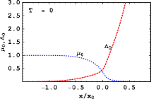
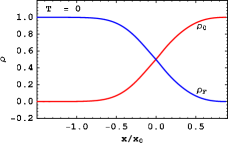
Figure 7: Crossover at zero temperature from the BCS regime (small $x$) to the BEC regime (large $x$). Left panel: fermion chemical potential $\mu_{0}$ (blue dotted) and gap $\Delta_{0}$ (red dashed) in units of effective Fermi energy $\epsilon_{F}$. Right panel: condensate fraction (red solid), fermion fraction (blue solid).

Let us discuss the quasi-fermion and quasi-antifermion excitation energies given by $\epsilon_{k}^{+}$ and $\epsilon_{k}^{-}$. Inserting the numerical solutions for $\mu$ and $\Delta$ into these energies results in the curves shown in Fig. 8. These excitation energies show that, for large values of $x$, quasi-fermions and quasi-antifermions become degenerate due to the vanishingly small chemical potential. Because of the large energy gap, we expect neither quasi-fermions nor quasi-antifermions to be present in the system.

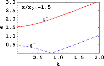
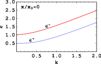
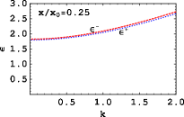
Figure 8: Fermion and antifermion excitation energies $\epsilon_{k}^{+}$ and $\epsilon_{k}^{-}$ for three different values of the crossover parameter $x/x_{0}$ at $T=0$ as a function of the momentum $k$ (both $\epsilon_{k}^{e}$ and $k$ are given in units of $\epsilon_{F}$). In the BCS regime (left panel) the energy gap is small and the fermion excitations are well separated from antifermion excitations. Both excitations approach each other in the unitary regime (middle panel), and become indistinguishable in the far BEC regime (right panel). Note in particular that the minimum of the antiparticle excitation is not a monotonic function of $x$.

The condensate and the fermion and boson density fractions at fixed crossover parameter $x/x_{0}=0.2$ are shown in Fig. 9. At the left end, $T=0$, one recovers the results shown in Fig. 7 at the particular value $x/x_{0}=0.2$, at the point $T/T_{c}=1$ the second-order phase transition manifests itself in a kink in the density fractions and a vanishing condensate. Below $T_{c}$ we observe coexistence of condensed bound states, condensed resonant states, and, for sufficiently large temperatures, uncondensed bound states. We obtain thermal bosons even above the phase transition. They can be interpreted as “preformed” pairs, just as the uncondensed pairs below $T_{c}$. This phenomenon is also called “pseudogap” in the literature [77]. It suggests that there is a temperature $T^{*}(x)$ which marks the onset of pair formation. This temperature is not necessarily identical to $T_{c}$. In the BCS regime, $T^{*}(x)=T_{c}(x)$, while for $x\gtrsim 0$, $T^{*}(x)>T_{c}(x)$. Of course, our model does not predict any quantitative value for $T^{*}$ because thermal bosons are present for all temperatures. Therefore, we expect the model to be valid only for a limited temperature range above $T_{c}$.

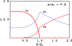
Figure 9: Density fractions in the crossover regime at fixed $x/x_{0}=0.2$ as functions of temperature: condensed bosons (red solid), fermions and uncondensed bosons (blue dotted and red dashed, respectively).

With the mean field appoximation, the boson-fermion model can be employed to describe the BCS-BEC crossover. An important property of the model is the coexistence of weakly-coupled Cooper pairs with condensed and uncondensed bosonic bound states. In the crossover regime as well as in the BEC regime, strongly-bound molecular Cooper pairs exist below and above the critical temperature $T_{c}$. Above $T_{c}$, they are all uncondensed (“preformed” Cooper pairs) while below $T_{c}$ a certain fraction of them forms a Bose-Einstein condensate. In contrast, in the BCS regime, pairing and condensation of fermionic degrees of freedom (in the absence of bosons) both set in at $T_{c}$.

It is straightforward to extend our boson-fermion model to two fermion species with cross-species pairing [120, 39]. This allows us to introduce a mismatch in fermion numbers and chemical potentials which imposes a stress on the pairing [121, 122]. This kind of stressed pairing takes place in a variety of real systems. For example, quark matter in a compact star is unlikely to exhibit standard BCS pairing in the color-flavor locked (CFL) phase, i.e., pairing of quarks at a common Fermi surface. The cross-flavor (and cross-color) pairing pattern of the CFL phase rather suffers a mismatch in chemical potentials in the pairing sectors $bu-rs$ and $bd-gs$ ($r,g,b$ meaning red, green, blue, and $u,d,s$ meaning up, down, strange). This mismatch is induced by the explicit flavor symmetry breaking through the heaviness of the strange quark and by the conditions of color and electric neutrality. Our system shall only be an idealized and simplified model of this complicated scenario. However, as in the previous sections, we shall allow for arbitrary values of the crossover parameter and thus model the strong coupling regime of quark matter. We shall fix the overall charge and the difference in the two charges. This is comparable to the effect of neutrality conditions for matter inside a compact star, which also impose constraints on the various color and flavor densities. Our focus will be to find stable homogeneous superfluids in the crossover region and, by discarding the unstable solutions, identify parameter values where the crossover in fact becomes a phase transition.

We denote the average chemical potential and the mismatch in chemical potentials by $\overline{\mu}\equiv\frac{\mu_{1}+\mu_{2}}{2},\,\delta\mu\equiv\frac{\mu_{1}-\mu_{2}}{2}.$ Then, the bosonic chemical potential is $\mu_{b}=2\overline{\mu}\,.$ The thermodynamic potential differs from the one-fermion case in the dispersion relation for the fermions,

$$\Omega = \frac{m_{b}^{2}-\mu_{b}^{2}}{4g^{2}}\Delta^{2}+\frac{1}{2}\sum_{e}\int\frac{d^{3}k}{(2\pi)^{3}}\left[\omega_{k}^{e}+2T\ln\left(1-e^{-\omega_{k}^{e}/T}\right)\right]$$ (184)

$$-\sum_{e}\int\frac{d^{3}k}{(2\pi)^{3}}\left\{\epsilon_{k}^{e}+T\ln\left[1+e^{-(\epsilon_{k}^{e}+\delta\mu)/T}\right]\right.$$

$$\left.+T\ln\left[1+e^{-(\epsilon_{k}^{e}-\delta\mu)/T}\right]\right\},$$

With coupled gap equaiton ($0=\frac{\partial\Omega}{\partial\Delta}$) and fixed sum ($\bar{n}\equiv n_{1}+n_{2}=-\frac{\partial\Omega}{\partial\bar{\mu}}$) and difference ($\delta n\equiv n_{1}-n_{2}=-\frac{\partial\Omega}{\partial\delta\mu}$) of the particle number density equations, the variables $\bar{\mu\,,}\,\delta\mu\>$ and$\Delta$ can be solved out.

In order to check the gapless states for their stability, we have to compute the number susceptibility matrix$\chi_{ij}\equiv\frac{dn_{i}}{d\mu_{j}}\,,\,i=1,2$. Note that we fix $\overline{n}$ and $\delta n$ (or equivalently $n_{1}$ and $n_{2}$) in our solution. Hence $\chi$ can be regarded as measuring the response of the system to a small perturbation away from this solution. In particular, a stable solution requires the mismatch in density to increase for an increasing mismatch in chemical potentials. Therefore, a negative eigenvalue of this 2$\times$2 matrix indicates the instability of a given solution.

We finally present a phase diagram in Fig. 10 for arbitrary (positive) values of $\delta n/\overline{n}$. Since we do not consider spatially inhomogeneous phases, this phase diagram is incomplete. Its main point is to identify regions where homogeneous gapless superfluids may exist. We find that for sufficiently large mismatches, $\delta n/\overline{n}\gtrsim 0.02$ there is a region where no solution with nonzero $\Delta$ can be found. We see that the region of stable superfluids shrinks with increasing $\delta n/\overline{n}$, as expected. Note that the horizontal axis$\delta n/\overline{n}=0$ is not continuously connected to the rest of the phase diagram. For vanishing mismatch in densities a stable, fully gapped superfluid exists for all $x$. One should thus not be misled by the instability for arbitrarily small mismatches.

We conclude with emphasizing the two main qualitative differences to analogous phase diagrams in nonrelativistic systems: $(i)$ within the stable region of homogeneous gapless superfluids there is a curve that separates two different Fermi surface topologies; this is the right dashed-dotted line in Fig. 10. $(ii)$ for large $x$ the gapless superfluid becomes unstable even in the far BEC region; this is the shaded area on the right side in Fig. 10.

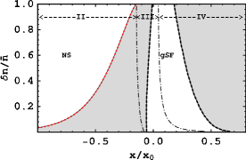
Figure 10: The phase diagram in the plane of the crossover parameter $x$ and the density difference $\delta n/\overline{n}$. Shaded areas have unstable homogeneous solutions with negative number susceptibility. NS denotes “normal state”; in this region, no solution for the gap equation is found. gSF denotes “gapless superfluid”; in this region a stable gapless superfluid state is found with two different Fermi surface topologies, divided by the right dashed-dotted line. Roman numbers II, III and IV denote three types of Fermi surface topologies [115].

13 Phenomenological implication: neutrino processes in compact stars

Generally the color superconducting quark matter cannot be easily produced in laboratory. The most possible place for the color superconductor is in the core of some compact stars where the high baryon density is realized. In recent years, people have been looking for the connection of color superconductivity to observations. The compact stars are born from supernova explosions where neutrino processes play crucial roles. Looking for evidences of color superconductivity from neutrino processes is a natural choice. One possible way is to study the compact star cooling through the neutrino emission, which is the major cooling process for proto-neutron stars and compact stars with relatively high internal temperature in the neutrino dominant stage. In this stage star bodies are transparent to neutrinos while opaque to photons. When the compact stars cool down by the neutrino emission, the photon emission gradually takes over for the later cooling. The compact star cooling models depend heavily on models for the neutron star interior especially the core. The star core could be nucleon matter, hyperon matter, pion or kaon condensate, or quark matter. There is huge amount of literature about compact star cooling since it was first studied by Tsuruta and Cameron in 1966 [123]. For a recent review of the neutron star cooling, see, e.g. [124]. For a review of neutron star evolution, see e.g. [125]. A recent systematic work in neutron star cooling based on hadronic models can be found in Ref. [126].

Figure 11: Neutrino processes in quark matter. (a) Urca; (b) Modified Urca; (c) Bremsstrahlung

(a)

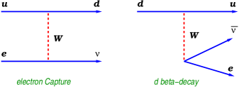
(b)

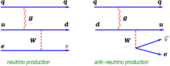
(c)

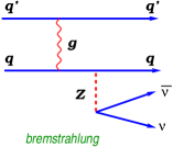
Calculating neutrino prcocesses in normal quark matter is part of effort to describe the cooling behavior of compact stars with quark matter cores. Roughly speaking there are three kinds of the neutrino prcocesses in quark matter: the Urca, the modified Urca and the bremsstrahlung processes, see Fig. (11). The first systematic and complete calculation for the Urca process in normal quark matter was done by Iwamoto addressing the importance of Fermi liquid behavior for relaxing the strict constraint of energy-momentum conservation [127]. The recent work by Schafer and Schwenzer [128] extends Iwamoto’s work by taking into account of the non-Fermi liquid behaviors [67, 68, 129, 130]. For the neutrino emission in fully gapped superconducting phases, the Urca process is exponentially suppressed [131, 132, 133, 134]. The possible relevant processes for the neutrino emission would be from the Goldstone mode [135] or from the pair breaking and recombination processes [136, 137]. For gapless phases the Urca processes are not suppressed and like in the normal quark matter [138, 139, 140, 141].

In this section we will use close-time-path method to derive the Kadnoff-Baym equation. Based on the Kadnoff-Baym equation, we will obtain the kinetic equation for the neutrino emissivity for the normal and superconducting quark matter. There are other applications of close-time-path method, see, e.g. Ref. [142, 143] in the transport equation of the quark gluon plasma. For the derivation of Kadnoff-Baym equation and kinetic equation for other neutrino processes in compact star, see, e.g. Ref. [144, 145]. If the neutron star has a color superconducting quark matter core which is in the so-called spin-1 A-phase, we will show that the neutrino emission is asymmetric in space.

13.1 Covariant Kadnoff-Baym equation

The two-point Green function for a fermion can be defined in the following way

$$iG(1,2)=\left\langle T[\psi_{H}(1)\overline{\psi}_{H}(2)]\right\rangle,$$

where ’1’ and ’2’ denote all indices including spatial coordinates of the two fields. $T$ is the causal time-ordering operator which orders an operator at an earlier time to the right of an operator at a later time. The field operators $\psi_{H}(t)$ and $\overline{\psi}_{H}(t)$ in the Heisenberg picture are related to those in the Schödinger picture by

$$\psi_{H}(t) = \exp[i\mathcal{H}(t-t_{0})]\psi_{S}(t)\exp[-i\mathcal{H}(t-t_{0})]$$

$$\overline{\psi}_{H}(t) = \exp[i\mathcal{H}(t-t_{0})]\overline{\psi}_{S}(t)\exp[-i\mathcal{H}(t-t_{0})],$$

where $\mathcal{H}$ is the Hamiltonian of the system.

Figure 12: Ordering along the close-time path in Green function.

In the same way, we can define the two-point Green function on the close-time path $C$ as shown in Fig. (12),

$$iG(1,2) = \left\langle T_{C}[\psi_{H}(1)\overline{\psi}_{H}(2)]\right\rangle$$ (185)

$$= \left\langle T_{C}\left\{\exp\left[i\int_{C}d^{4}x\mathcal{L}^{\prime}_{I}\right]\psi_{I}(1)\overline{\psi}_{I}(2)\right\}\right\rangle,$$

where $\mathcal{L}^{\prime}_{I}$ is the interacting part of the Lagrangian in the interaction picture and $T_{C}$ is the ordering operator along the close-time path $C$. $G(1,2)$ can be written as

$$G(1,2)=\Theta_{C}(t_{1}-t_{2})G^{>}(1,2)+\Theta_{C}(t_{2}-t_{1})G^{<}(1,2),$$ (186)

where $G^{>,<}$ are correlation functions. We also need the retarded and advanced Green functions as follows

$$G^{R}(1,2) = G(1,2)-G^{<}(1,2)=\Theta_{C}(t_{1}-t_{2})[G^{>}(1,2)-G^{<}(1,2)]$$

$$G^{A}(1,2) = G(1,2)-G^{>}(1,2)=\Theta_{C}(t_{2}-t_{1})[G^{<}(1,2)-G^{>}(1,2)].$$

The series expansion of the exponential function in Eq. (185) generates the perturbation expansion for the two-point Green function. In lowest order one obtains the non-interacting Green function $G_{0}$ whose inverse $G_{0}^{-1}$ is

$$G_{0}^{-1}(1,2)=(i\gamma_{\mu}\partial_{1}^{\mu}-m)\delta(1,2).$$

The relation between a Green function and its inverse is

$$\int_{C}d3G^{-1}(1,3)G(3,2)=\int_{C}d3G(1,3)G^{-1}(3,2)=\delta(1,2).$$

Dyson-Schwinger equation is

$$G^{-1}(1,2) = G_{0}^{-1}(1,2)-\Sigma(1,2),$$ (187)

which can be further written as

$$G_{0}^{-1}G = 1+\Sigma G$$

$$GG_{0}^{-1} = 1+G\Sigma,$$ (188)

whose explicit form is

$$(i\gamma_{\mu}\partial_{1}^{\mu}-m)G(1,2) = \delta(1,2)+\int_{C}d3\Sigma(1,3)G(3,2)$$ (189)

$$G(1,2)(-i\gamma_{\mu}\overleftarrow{\partial}_{2}^{\mu}-m) = \delta(1,2)+\int_{C}d3G(1,3)\Sigma(3,2),$$ (190)

After simplification by translating the contour integrals into normal ones we get Dyson-Schwinger equations

$$(i\gamma_{\mu}\partial_{1}^{\mu}-m)G^{<}(1,2) = -\int_{t_{0}}^{t_{2}}d3\Sigma^{<}(1,3)\left[G^{>}(3,2)-G^{<}(3,2)\right]$$ (191)

$$-\int_{t_{0}}^{t_{1}}d3\left[\Sigma^{<}(1,3)-\Sigma^{>}(1,3)\right]G^{<}(3,2),$$

$$G^{<}(1,2)(-i\gamma_{\mu}\overleftarrow{\partial}_{2}^{\mu}-m) = -\int_{t_{0}}^{t_{2}}d3G^{<}(1,3)\left[\Sigma^{>}(3,2)-\Sigma^{<}(3,2)\right]$$ (192)

$$-\int_{t_{0}}^{t_{1}}d3\left[G^{<}(1,3)-G^{>}(1,3)\right]\Sigma^{<}(3,2),$$

where we have used the correlation parts of the self-energy $\Sigma^{>}$ and $\Sigma^{<}$ in analogy to Eq. (186). Making gradient expansion and Fourier transformation, taking the difference of the above two Dyson-Schwinger equations, and finally taking traces for the resulting equations, we obtain Kadanoff-Baym equation

$$\partial_{X}^{\mu}\mathrm{Tr}[\gamma_{\mu}iG^{<}(X,P)]=-\mathrm{Tr}\left[iG^{>}(-i\Sigma^{<})-(-i\Sigma^{>})iG^{<}\right](X,P).$$ (193)

where $X=(X_{1}+X_{2})/2$ and $P$ is the momentum variable conjugate to $X$. Note that our convention for the sign of selfenergy is implied in $G^{-1}=G^{(0)-1}-\Sigma$, which means $-i\Sigma$ in the Feynman rules.

13.2 Kinetic equation

We can derive the kinetic equation from Eq. (193). The fermionic Green functions (here we mean the electron and the neutrino or their anti-particles) can be expressed in terms of distribution functions as follows

$$iG^{<}(X,P) = -\gamma^{\mu}P_{\mu}\frac{\pi}{p}\left\{f_{e^{-}/\nu}(t,\mathbf{p})\delta(p_{0}+\mu_{e^{-}/\nu}-p)\right.$$ (194)

$$\left.-[1-f_{e^{+}/\overline{\nu}}(t,-\mathbf{p})]\delta(p_{0}+\mu_{e^{-}/\nu}+p)\right\}.$$

where we have shifted $p_{0}$ by the chemical potential $p_{0}\rightarrow p_{0}+\mu_{e^{-}/\nu}$. In the same way, we can obtain $G^{>}$ as follows

$$iG^{>}(X,P) = \gamma^{\mu}P_{\mu}\frac{\pi}{p}\left\{[1-f_{e^{-}/\nu}(t,\mathbf{p})]\delta(p_{0}+\mu_{e^{-}/\nu}-p)\right.$$ (195)

$$\left.-f_{e^{+}/\overline{\nu}}(t,-\mathbf{p})\delta(p_{0}+\mu_{e^{-}/\nu}+p)\right\}.$$

We assume that the distribution function $f$ only depends on $X_{0}=t$, so that $G(X,P)$ can be written as $G(t,P)$. This approximation is well justified for neutrinos in the compact star with mean free paths comparable or larger than size of the star.

We are interested in the neutrino cooling stage in the compact star. When neutrinos are produced they escape the star immediately. The neutrino density can not be built up in the star. So we can put the chemical potentials of the neutrino and anti-neutrino zero. Substituting Eq. (194) and (195) into Eq. (196), and carrying out the integral $\int_{0}^{\infty}dp_{0}$, we obtain the equation for the time variation rate of the neutrino distribution:

$$\frac{\partial}{\partial t}f_{\nu}(t,\mathbf{p}) = \frac{1}{4\pi}\int_{0}^{\infty}dp_{0}\mathrm{Tr}\left[iG_{\nu}^{>}(-i\Sigma_{\nu}^{<})\right.$$ (196)

$$\left.-(-i\Sigma_{\nu}^{>})iG_{\nu}^{<}\right](t,P),$$

which picks up the contribution corresponding to the term with support at $p_{0}=p$ in the left hand side. In the same way, we can extract the kinetic equation for the anti-neutrinos by carrying out the integral $\int_{-\infty}^{0}dp_{0}$

$$\frac{\partial}{\partial t}f_{\overline{\nu}}(t,-\mathbf{p}) = -\frac{1}{4\pi}\int_{-\infty}^{0}dp_{0}\mathrm{Tr}\left[iG_{\overline{\nu}}^{>}(-i\Sigma_{\overline{\nu}}^{<})\right.$$ (197)

$$\left.-(-i\Sigma_{\overline{\nu}}^{>})iG_{\overline{\nu}}^{<}\right](t,P),$$

which picks up the contribution corresponding to the term with support at $p_{0}=-p$.

In order to evaluate $\Sigma^{>,<}$, we need the Feynman diagram as shown in Fig. (13). The convention about the order of fermionic fields in the Feynman diagram is along the direction of momentum flow. From the diagram Fig. (13)(a), the neutrino self-energy reads:

Figure 13: Self-energy in close-time-path formalism for the neutrino Urca process.

\psfrag{dquark}{$d$}\psfrag{uquark}{$u$}\psfrag{q-mom}{$Q$}\psfrag{wboson}{$W$}\psfrag{nu_e}{$\nu_{e}$}\psfrag{e-}{$e^{-}$}\psfrag{nu}{$\nu$}\psfrag{nu1}{$\nu^{\prime}$}\psfrag{mu}{$\mu$}\psfrag{mu1}{$\mu^{\prime}$}\psfrag{P1}{$P_{e}$}\psfrag{P2}{$P_{d}$}\psfrag{P3}{$P_{u}$}\psfrag{p-mom}{$P_{\nu}$}\includegraphics[scale={0.5}]{trino32}

$$-i\Sigma_{\nu}^{<}(P_{\nu}) = -\int\frac{d^{4}P_{e}}{(2\pi)^{4}}(-i\Gamma_{e}^{\mu})iG_{e}^{<}(P_{e})i\Gamma_{e}^{\nu}$$

$$\times[-i\Pi_{\mu^{\prime}\nu^{\prime}}^{>}(P_{e}-P_{\nu})]iD_{\mu}^{\overline{F},\mu^{\prime}}(P_{e}-P_{\nu})iD_{\nu}^{F,\nu^{\prime}}(P_{e}-P_{\nu})$$

$$= \frac{G_{F}^{2}}{2}\int\frac{d^{4}P_{e}}{(2\pi)^{4}}\gamma^{\mu}(1-\gamma_{5})\gamma^{\sigma}P_{e,\sigma}\gamma^{\nu}(1-\gamma_{5})$$

$$\times[-i\Pi_{\mu\nu}^{>}(P_{e}-P_{\nu})]\frac{\pi}{p_{e}}f_{e}(t,\mathbf{p}_{e})\delta(p^{\prime}_{e0}-p_{e}),$$

where the overall sign is due to the quark loop. Note that $P_{e}\equiv(p^{\prime}_{e0},\mathbf{p}_{e})$ with $p^{\prime}_{e0}\equiv p_{e0}+\mu_{e}$, then integral element is $d^{4}P_{e}\equiv dp^{\prime}_{e0}d^{3}\mathbf{p}_{e}$. We have defined the order of ’>’ and ’<’ in $\Pi^{>,<}$ along the momentum direction. For example, in the first Feynman diagram Fig. (13)(a), the W-boson polarization tensor is defined by from $\mu^{\prime}$ to $\nu^{\prime}$ following the momentum flow, i.e. $\mu^{\prime}$ as the first entry and $\nu^{\prime}$ as the second one. The first entry on the negative branch has a time later than the first entry on the close-time-path contour $C$. Therefore we have $\Pi_{\mu^{\prime}\nu^{\prime}}^{>}$. In the same way, Fig. (13)(b) reads

$$-i\Sigma_{\nu}^{>}(P_{\nu}) = -\int\frac{d^{4}P_{e}}{(2\pi)^{4}}i\Gamma_{e}^{\mu}iG_{e}^{>}(P_{e})(-i\Gamma_{e}^{\nu})$$

$$\times[-i\Pi_{\mu^{\prime}\nu^{\prime}}^{<}(P_{e}-P_{\nu})]iD_{\mu}^{F,\mu^{\prime}}(P_{e}-P_{\nu})iD_{\nu}^{\overline{F},\nu^{\prime}}(P_{e}-P_{\nu})$$

$$= -\frac{G_{F}^{2}}{2}\int\frac{d^{4}P_{e}}{(2\pi)^{4}}\gamma^{\mu}(1-\gamma_{5})\gamma^{\sigma}P_{e,\sigma}\gamma^{\nu}(1-\gamma_{5})$$

$$\times[-i\Pi_{\mu\nu}^{<}(P_{e}-P_{\nu})]\frac{\pi}{p_{e}}[1-f_{e}(t,\mathbf{p}_{e})]\delta(p^{\prime}_{e0}-p_{e}).$$

Inserting $-i\Sigma_{\nu}^{>}(P_{\nu})$ and $-i\Sigma_{\nu}^{<}(P_{\nu})$ into Eq. (196), we get

$$\frac{\partial}{\partial t}f_{\nu}(t,\mathbf{p}_{\nu}) = \frac{1}{4\pi}\frac{G_{F}^{2}}{2}\int\frac{d^{3}\mathbf{p}_{e}}{(2\pi)^{4}}\frac{\pi}{p_{\nu}}\frac{\pi}{p_{e}}L^{\mu\nu}(P_{\nu},P_{e})$$ (198)

$$\times[1-f_{\nu}(t,\mathbf{p}_{\nu})]f_{e}(t,\mathbf{p}_{e})[-i\Pi_{\mu\nu}^{>}(P_{e}-P_{\nu})],$$

where $P_{\nu}=(p_{\nu},\mathbf{p}_{\nu})$ and $P_{e}=(p_{e},\mathbf{p}_{e})$. Note that the definition for $P_{e}$ has been changed from the original one. The leptonic tensor $L^{\mu\nu}$ is defined by

$$L^{\mu\nu}(P_{\nu},P_{e})\equiv\mathrm{Tr}\left[\gamma^{\lambda}P_{\nu,\lambda}\gamma^{\mu}(1-\gamma_{5})\gamma^{\sigma}P_{e,\sigma}\gamma^{\nu}(1-\gamma_{5})\right].$$

For the anti-neutrino, we still use $P$ to denote its momentum, only the second term $\sim(-i\Sigma_{\overline{\nu}}^{>})iG_{\overline{\nu}}^{<}$ in Eq. (197) contributes. Finally we obtain

$$\frac{\partial}{\partial t}f_{\overline{\nu}}(t,-\mathbf{p}_{\overline{\nu}}) = -\frac{1}{4\pi}\frac{G_{F}^{2}}{2}\int\frac{d^{3}\mathbf{p}_{e}}{(2\pi)^{4}}\frac{\pi}{p_{\overline{\nu}}}\frac{\pi}{p_{e}}L^{\mu\nu}(P_{\overline{\nu}},P_{e})$$ (199)

$$\times[1-f_{\overline{\nu}}(-\mathbf{p}_{\overline{\nu}})][1-f_{e}(\mathbf{p}_{e})][-i\Pi_{\mu\nu}^{<}(P_{e}-P_{\overline{\nu}})],$$

where $P_{\overline{\nu}}=(-p_{\overline{\nu}},\mathbf{p}_{\overline{\nu}})$. We can rewrite Eq. (199) by flipping the momentum sign: $\mathbf{p}_{\overline{\nu}}\rightarrow-\mathbf{p}_{\overline{\nu}}$,

$$\frac{\partial}{\partial t}f_{\overline{\nu}}(t,\mathbf{p}_{\overline{\nu}}) = -\frac{1}{4\pi}\frac{G_{F}^{2}}{2}\int\frac{d^{3}\mathbf{p}_{e}}{(2\pi)^{4}}\frac{\pi}{p_{\overline{\nu}}}\frac{\pi}{p_{e}}L^{\mu\nu}(P_{\overline{\nu}},P_{e})$$ (200)

$$\times[1-f_{\overline{\nu}}(\mathbf{p}_{\overline{\nu}})][1-f_{e}(\mathbf{p}_{e})][-i\Pi_{\mu\nu}^{<}(P_{e}-P_{\overline{\nu}})],$$

where $P_{\overline{\nu}}$ is changed to $P_{\overline{\nu}}=(-p_{\overline{\nu}},-\mathbf{p}_{\overline{\nu}})$. We will see that the negative sign in front of Eq. (200) will cancel the negative sign due to $P_{\overline{\nu}}=(-p_{\overline{\nu}},-\mathbf{p}_{\overline{\nu}})$ in the matrix element. Thus the result for the anti-neutrino is the identical to the neutrino.

Using the following relations between $\Pi_{\mu\nu}^{>}$ and $\Pi_{\mu\nu}^{R}$

$$\Pi^{<}(K) = -2in_{B}(k_{0})\mathrm{Im}\Pi^{R}(K)$$

$$\Pi^{>}(K) = -2i[1+n_{B}(k_{0})]\mathrm{Im}\Pi^{R}(K),$$

where $n_{B}(k_{0})=1/(e^{\beta k_{0}}-1)$ is the Bose-Einstein distribution, Eq. (198) can be expressed in terms of $\mathrm{Im}\Pi^{R}(P_{e}-P_{\nu})$ as

$$\frac{\partial}{\partial t}f_{\nu}(t,\mathbf{p}_{\nu}) = \frac{1}{4\pi}G_{F}^{2}\int\frac{d^{3}\mathbf{p}_{e}}{(2\pi)^{4}}\frac{\pi}{p_{\nu}}\frac{\pi}{p_{e}}L^{\mu\nu}(P_{\nu},P_{e})n_{B}(p_{\nu}-p_{e}+\mu_{e})$$

$$\times[1-f_{\nu}(t,\mathbf{p}_{\nu})]f_{e}(t,\mathbf{p}_{e})\mathrm{Im}\Pi_{\mu\nu}^{R}(P_{e}-P_{\nu}),$$

where we have used $n_{B}(k_{0})+n_{B}(-k_{0})=-1$. Taking the momentum integral $\frac{d^{3}\mathbf{p}_{\nu}}{(2\pi)^{3}}$ and noting that $n_{\nu}=\int\frac{d^{3}\mathbf{p}_{\nu}}{(2\pi)^{3}}f_{\nu}(t,\mathbf{p}_{\nu})$, we obtain the number emissivity per volume for neutrinos:

$$\frac{\partial}{\partial t}n_{\nu}(t) = \frac{1}{2}G_{F}^{2}\int\frac{d^{3}\mathbf{p}_{e}}{(2\pi)^{3}}\frac{d^{3}\mathbf{p}_{\nu}}{(2\pi)^{3}}\frac{1}{2p_{\nu}}\frac{1}{2p_{e}}L^{\mu\nu}(P_{\nu},P_{e})n_{B}(p_{\nu}-p_{e}+\mu_{e})$$ (201)

$$\times[1-f_{\nu}(t,\mathbf{p}_{\nu})]f_{e}(t,\mathbf{p}_{e})\mathrm{Im}\Pi_{\mu\nu}^{R}(P_{e}-P_{\nu}).$$

The emissivity for anti-neutrinos is the same as that of neutrinos. The energy emissivity can be obtained by including $p_{\nu}$ into the integrand in Eq. (201).

13.3 u-d-W vertex in Nambu-Gorkov basis

Because we are interested in Urca processes, we have to write down the u-d-W interaction vertex in NG basis. The u-d-W vertex differs from the quark-gluon one in Nambu-Gorkov forms due to the flavor changing nature of the W-boson interaction. So we explicitly keep the flavor indices $f$ for the quark fields:

$$\psi_{C}(f)=C\overline{\psi}^{T}(f),\;\overline{\psi}_{C}(f)=\psi^{T}(f)C$$

$$\psi(f)=C\overline{\psi}_{C}^{T}(f),\;\overline{\psi}(f)=\psi_{C}^{T}(f)C.$$

where we assume $f=1,2$ for $u,d$ respectively. We need for the u-d-W coupling an additional flavor matrix $\tau_{\pm}$ to guarantee that $W^{\pm}$ couples to $u$ and $d$ instead of the same flavor, where $\tau_{\pm}$ are defined by

$$\tau_{+}=\left(\begin{array}[]{cc}0&1\\ 0&0\end{array}\right),\;\tau_{-}=\left(\begin{array}[]{cc}0&0\\ 1&0\end{array}\right).$$

Here we assume the spinor order of the vertex is $d-W^{-}-u$ and $u-W^{+}-d$, where the momenta of W-bosons flow into vertices, see Fig. (14). Then we have

$$i\Gamma_{\pm}^{\mu} = -\frac{ie}{2\sqrt{2}\sin\theta_{W}}\gamma^{\mu}(1-\gamma_{5})\tau_{\pm},$$

where $\theta_{W}$ is the Weinberg’s angle. Here we have taken CKM matrix element for $u$ and $d$ quark $V_{ud}\approx 1$. The Fermi weak coupling constant $G_{F}$ is related to $\theta_{W}$ by $\frac{G_{F}}{\sqrt{2}}=\frac{e^{2}}{8M^{2}\sin^{2}\theta_{W}}$.

Figure 14: u-d-W vertices. The momenta of W-bosons flow into the vertices.

\psfrag{W-}{$W^{-}$}\psfrag{V-}{$i\Gamma^{NG}_{-}$}\psfrag{W+}{$W^{+}$}\psfrag{V+}{$i\Gamma^{NG}_{+}$}\includegraphics{neutrino-vertex}

Then we can write down the u-d-W interaction term

$$\overline{\psi}(f_{1})\Gamma_{\pm}^{\mu}\psi(f_{2}) = \psi_{C}^{T}(f_{1})C\Gamma_{\pm}^{\mu}C\overline{\psi}_{C}^{T}(f_{2})$$

$$= -\left[\overline{\psi}_{C}(f_{2})C^{T}\Gamma_{\pm}^{\mu T}C^{T}\psi_{C}(f_{1})\right]^{T}$$

$$= -\overline{\psi}_{C}(f_{2})C^{T}\Gamma_{\pm}^{\mu T}C^{T}\psi_{C}(f_{1})$$

$$\equiv \overline{\psi}_{C}(f_{2})\overline{\Gamma}_{\pm}^{\mu}\psi_{C}(f_{1}),$$

where we have defined $\overline{\Gamma}_{\pm}^{\mu}\equiv-C\Gamma_{\pm}^{\mu T}C$. Therefore the u-d-W vertex in Nambu-Gorkov basis is given by

$$i\Gamma_{\pm;NG}^{\mu} = -\frac{ie}{2\sqrt{2}\sin\theta_{W}}\left(\begin{array}[]{cc}\gamma^{\mu}(1-\gamma_{5})\tau_{\pm}&0\\ 0&-\gamma^{\mu}(1+\gamma_{5})\tau_{\mp}\end{array}\right)$$ (204)

$$\equiv -\frac{ie}{2\sqrt{2}\sin\theta_{W}}\Gamma_{NG}^{\mu}\tau_{\pm;NG},$$ (205)

where we have defined

$$\Gamma_{NG}^{\mu} \equiv \left(\begin{array}[]{cc}\gamma^{\mu}(1-\gamma_{5})&0\\ 0&-\gamma^{\mu}(1+\gamma_{5})\end{array}\right),\;\tau_{\pm;NG}\equiv\left(\begin{array}[]{cc}\tau_{\pm}&0\\ 0&\tau_{\mp}\end{array}\right).$$

13.4 Polarization tensor for W-boson from quark loop in superconducting phase

Now we can calculate the polarization tensor $\Pi_{\mu\nu}(Q)$ for the W-boson from the quark loop in imaginary time formalism for superconducting phases. Here $Q=P_{e}-P_{\nu}$. Then we make analytical extension to get retarded polarization tensor. The quark propagator with condensate can be written as $\mathcal{G}_{ij}=\mathcal{G}_{ij}^{u}\tau_{11}+\mathcal{G}_{ij}^{d}\tau_{22}$ where $i,j$ are Nambu-Gorkov indices and $\tau_{11}=\mathrm{diag}(1,0)$ and $\tau_{22}=\mathrm{diag}(0,1)$ in the flavor space of $u$ and $d$ quark. $\mathcal{G}_{ij}^{u}$ and $\mathcal{G}_{ij}^{d}$ are given by Eq. (115). Let’s look at one case where the left vertex is $\tau_{-;NG}$ while the right must be $\tau_{+;NG}$, as illustrated corresponding to the fermion loop direction in Fig. (13). Then the polarization tensor of the W-boson in imaginary time formalism reads

$$\Pi^{\mu\nu}(Q) = \frac{1}{2}T\sum_{p_{u0}}\int\frac{d^{3}\mathbf{p}_{u}}{(2\pi)^{3}}\mathrm{Tr}_{NG,c,f,s}[\Gamma_{NG}^{\mu}\tau_{-;NG}\mathcal{G}^{u}(P_{u})\Gamma_{NG}^{\nu}\tau_{+NG}\mathcal{G}^{d}(P_{d})]$$ (207)

$$= \frac{1}{2}T\sum_{p_{u0}}\int\frac{d^{3}\mathbf{p}_{u}}{(2\pi)^{3}}\mathrm{Tr}_{c,f,s}[\gamma^{\mu}(1-\gamma_{5})\tau_{-}\mathcal{G}_{11}^{u}(P_{u})$$

$$\times\gamma^{\nu}(1-\gamma_{5})\tau_{+}\mathcal{G}_{11}^{d}(P_{d})]$$

$$+\frac{1}{2}T\sum_{p_{u0}}\int\frac{d^{3}\mathbf{p}_{u}}{(2\pi)^{3}}\mathrm{Tr}_{c,f,s}[\gamma^{\mu}(1+\gamma_{5})\tau_{+}\mathcal{G}_{22}^{u}(P_{u})$$

$$\times\gamma^{\nu}(1+\gamma_{5})\tau_{-}\mathcal{G}_{22}^{d}(P_{d})]$$

$$-\frac{1}{2}T\sum_{p_{u0}}\int\frac{d^{3}\mathbf{p}_{u}}{(2\pi)^{3}}\mathrm{Tr}_{c,f,s}[\gamma^{\mu}(1-\gamma_{5})\tau_{-}\mathcal{G}_{12}^{u}(P_{u})$$

$$\times\gamma^{\nu}(1+\gamma_{5})\tau_{-}\mathcal{G}_{21}^{d}(P_{d})]$$

$$-\frac{1}{2}T\sum_{p_{u0}}\int\frac{d^{3}\mathbf{p}_{u}}{(2\pi)^{3}}\mathrm{Tr}_{c,f,s}[\gamma^{\mu}(1+\gamma_{5})\tau_{+}\mathcal{G}_{21}^{u}(P_{u})$$

$$\times\gamma^{\nu}(1-\gamma_{5})\tau_{+}\mathcal{G}_{12}^{d}(P_{d})].$$

where $P_{d}\equiv P_{u}+Q$, and $p_{u0}=-i(2l+1)\pi T$ with integer $l$ are Matsubara frequencies. The order in the trace is against the direction of fermion line in Fig. (13). The last two terms in Eq. (207) proportional to the off-diagonal propagators are zero due to the presence of two identical $\tau_{-}$ or $\tau_{+}$ leading to vanishing flavor traces. This a spectacular feature for single flavor pairing. Taking the flavor trace and Matsubara sum, and noting that the first and second terms are identical, we obtain

$$\Pi^{\mu\nu}(Q) = T\sum_{p_{u0}}\int\frac{d^{3}\mathbf{p}_{u}}{(2\pi)^{3}}Tr_{c,s}[\gamma^{\mu}(1-\gamma_{5})\mathcal{G}_{11}^{u}(P_{u})\gamma^{\nu}(1-\gamma_{5})\mathcal{G}_{11}^{d}(P_{d})]$$ (208)

$$= \int\frac{d^{3}\mathbf{p}_{u}}{(2\pi)^{3}}\mathrm{Tr}_{c,s}[\gamma^{\mu}(1-\gamma_{5})\gamma_{0}\mathcal{P}^{r_{u}}\Lambda_{\mathbf{p}_{u}}^{-e_{u}}\gamma^{\nu}(1-\gamma_{5})\gamma_{0}\mathcal{P}^{r_{d}}\Lambda_{\mathbf{p}_{d}}^{-e_{d}}]$$

$$\times\left\{\left[\frac{n_{u}(1-n_{d})}{-q_{0}+\epsilon_{u}+\epsilon_{d}}-\frac{(1-n_{u})n_{d}}{-q_{0}-\epsilon_{u}-\epsilon_{d}}\right]\left[1-n_{F}(\epsilon_{u})-n_{F}(\epsilon_{d})\right]\right.$$

$$\left.+\left[\frac{(1-n_{u})(1-n_{d})}{-q_{0}-\epsilon_{u}+\epsilon_{d}}-\frac{n_{u}n_{d}}{-q_{0}+\epsilon_{u}-\epsilon_{d}}\right]\left[n_{F}(\epsilon_{u})-n_{F}(\epsilon_{d})\right]\right\}$$

where $\mathcal{P}^{r_{u}}$ is the projector corresponding to the excitation branch with index $r_{u}$. A sum over the excitation branch $r_{u}$ is implied (the function inside the curly brackets depends on the excitation branch $r_{u}$). $\Lambda_{\mathbf{p}}^{e}$ is the energy projector defined by $\Lambda_{\mathbf{p}}^{e}=(1-e\gamma_{0}\widehat{\mathbf{p}}\cdot\bm{\gamma})/2$. $n$ and $1-n$ are Bogoliubov coefficients for quasi-hole and quasi-particle respectively. They are given by

$$B_{-}\equiv n = \frac{1}{2}-\frac{\xi}{2\epsilon}$$

$$B_{+}\equiv 1-n = \frac{1}{2}+\frac{\xi}{2\epsilon}$$ (209)

where $\xi=k-e\mu$ and $\epsilon=\sqrt{\xi^{2}+\phi^{2}}$. Note that the gap parameter $\phi$ depends on the excitation branch. In Eq. (208) we only keep particle excitations, i.e. with $e_{u}=e_{d}=+$. For the derivation of the Matsubara sum, see, for example, [87, 146].

Then we are in the position of obtaining the imaginary part of the retarded polarization tensor $\mathrm{Im}\Pi_{R}^{\mu\nu}$ by making analytic extension $q_{0}\rightarrow q_{0}-i\delta$ in Eq. (207):

$$\mathrm{Im}\Pi_{R}^{\mu\nu}(Q) = \pi\int\frac{d^{3}\mathbf{p}_{u}}{(2\pi)^{3}}\mathrm{Tr}_{c,s}[\gamma^{\mu}(1-\gamma_{5})\gamma_{0}\mathcal{P}^{r_{u}}\Lambda_{\mathbf{p}_{u}}^{-}\gamma^{\nu}(1-\gamma_{5})\gamma_{0}\mathcal{P}^{r_{d}}\Lambda_{\mathbf{p}_{d}}^{-}]$$ (210)

$$\times n_{B}^{-1}(-q_{0})B_{a_{u}}B_{a_{d}}\delta(-q_{0}-a_{u}\epsilon_{u}+a_{d}\epsilon_{d})$$

$$\times n_{F}(a_{u}\epsilon_{u})[1-n_{F}(a_{d}\epsilon_{d})],$$

where $a$ denotes the nature of the excitations: $a=+$ for quasi-particles and $a=-$ for quasi-holes. The factor $n_{B}^{-1}(-q_{0})$ will cancel $n_{B}(p-p_{1}+\mu_{e})$ in Eq. (201). A sum over $a_{u}$ and $a_{d}$ is implied.

13.5 Evaluation of neutrino emissivity

Substituting Eq. (210) into Eq. (201), we get the number emissivity for neutrinos:

$$\frac{\partial}{\partial t}n_{\nu} = 2\pi\int\frac{d^{3}\mathbf{p}_{\nu}}{(2\pi)^{3}2p_{\nu}}\frac{d^{3}\mathbf{p}_{e}}{(2\pi)^{3}2p_{e}}\frac{d^{3}\mathbf{p}_{u}}{(2\pi)^{3}2p_{u}}\frac{1}{2p_{d}}|M|^{2}$$ (211)

$$\times B_{a_{u}}B_{a_{d}}\delta[p_{\nu}-(p_{e}-\mu_{e})-a_{1}\epsilon_{1}^{u}+a_{2}\epsilon_{2}^{d}]$$

$$\times n_{F}(p_{e}-\mu_{e})n_{F}(a_{u}\epsilon_{u})[1-n_{F}(a_{d}\epsilon_{d})].$$

We have defined the matrix element

$$|M|^{2} = G_{F}^{2}p_{u}p_{d}\mathrm{Tr}_{c,s}[\gamma^{\mu}(1-\gamma_{5})\gamma_{0}\mathcal{P}^{r_{u}}\Lambda_{\mathbf{p}_{u}}^{-}$$ (212)

$$\times\gamma^{\nu}(1-\gamma_{5})\gamma_{0}\mathcal{P}^{r_{d}}\Lambda_{\mathbf{p}_{d}}^{-}]L_{\mu\nu}(P_{\nu},P_{e})$$

$$\approx G_{F}^{2}\mathrm{Tr}_{c,s}[\gamma^{\mu}(1-\gamma_{5})\gamma_{0}\mathcal{P}^{r_{u}}P_{u,\sigma}\gamma^{\sigma}$$

$$\times\gamma^{\nu}(1-\gamma_{5})\gamma_{0}\mathcal{P}^{r_{d}}P_{d,\rho}\gamma^{\rho}]L_{\mu\nu}(P_{\nu},P_{e})$$

where we have used the mass-shell condition for the $u$ and $d$ quark. The energy emissivity for the e-capture process is then

$$\frac{\partial E_{\nu}}{\partial t} = 2\pi\int\frac{d^{3}\mathbf{p}_{\nu}}{(2\pi)^{3}2p_{\nu}}\frac{d^{3}\mathbf{p}_{e}}{(2\pi)^{3}2p_{e}}\frac{d^{3}\mathbf{p}_{u}}{(2\pi)^{3}2p_{u}}\frac{1}{2p_{d}}|M|^{2}p_{\nu}$$ (213)

$$\times B_{a_{u}}B_{a_{d}}\delta[p_{\nu}-(p_{e}-\mu_{e})-a_{u}\epsilon_{u}+a_{d}\epsilon_{d}]$$

$$\times n_{F}(p_{e}-\mu_{e})n_{F}(a_{u}\epsilon_{u})[1-n_{F}(a_{d}\epsilon_{d})].$$

One can also obtain the time rate for the momentum emitted along any direction by replacing $p_{\nu}$ with $p_{\nu}\cos\theta$, where $\theta$ is the angle between the neutrino momentum and this direction.

Figure 15: Phase space for Urca process.

\psfrag{d}{$d$}\psfrag{u}{$u$}\psfrag{e}{$e$}\psfrag{mu_u}{$\mu_{u}$}\psfrag{mu_d}{$\mu_{d}$}\psfrag{mu_e}{$\mu_{e}$}\psfrag{pd}{$p^{F}_{d}$}\psfrag{pu}{$p^{F}_{u}$}\psfrag{pe}{$p^{F}_{e}$}\psfrag{pf_e=mu_e}{$p^{F}_{e}=\mu_{e}$}\psfrag{pf=(1-xi)mu}{$p^{F}_{u,d}=(1-\frac{C_{F}\alpha_{s}}{2\pi})\mu_{u,d}$}\psfrag{cos(theta_ue)}{$\mathrm{cos}\theta_{ue}\approx 1-\frac{C_{F}\alpha_{s}}{2\pi}$}\psfrag{cos(theta_ud)}{$\mathrm{cos}\theta_{ud}\approx 1-\frac{C_{F}\alpha_{s}}{2\pi}\frac{\mu_{e}^{2}}{\mu_{u}\mu_{d}}$}\includegraphics[scale={0.7}]{neutrino-kinetics}

Before we evaluate Eq. (213), we analyze the phase space given by the energy conservation for quasi-particles, i.e. restricted by the delta function. If we don’t take any interactions into account, for excitations near the Fermi surface, the energy conservation condition reads

$$0 = p_{\nu}-(p_{e}-\mu_{e})-a_{u}\epsilon_{u}+a_{d}\epsilon_{d}$$

$$\approx p_{\nu}-a_{u}\phi_{u}+a_{d}\phi_{d}$$

$$\approx p_{\nu},$$

where we have used $p_{i}\approx\mu_{i}$ for $i=u,d,e$ and $p_{\nu}\gg\phi_{u,d}$. We see in the above equation that in order to make the energy conserved, the neutrino energy must vanish, which means the phase space for the neutrino emission is very much suppressed. So including the interactions for quasi-particles is necessary. The Fermi liquid correction to the non-interacting degenerate Fermi gas is a better description of interacting degenerate Fermi gas, which opens the phase space for neutrino emission. The Fermi liquid correction to the quark Fermi momentum is due to the quark-quark scattering via gluon exchange. The effect is that it reduces the Fermi momentum by an amount linearly proportional to the strong coupling constant as below:

$$p_{Fi} = (1-\frac{C_{F}\alpha_{S}}{2\pi})\mu_{Fi},$$

where $i=u,d$. Actually the Fermi liquid corrections make it possible to form the triangle by $p_{Fu}$, $p_{Fd}$ and $p_{Fe}$, as shown in Fig. (15). We can then determine the angles $\theta_{ud}$, $\theta_{ue}$ and $\theta_{de}$ by the triangle relation. For example, $\cos\theta_{ud}$ is given by

$$\cos\theta_{ud} = \frac{p_{Fd}^{2}+p_{Fu}^{2}-p_{Fe}^{2}}{2p_{Fu}p_{Fd}}$$

$$\approx \frac{(\mu_{d}^{2}+\mu_{u}^{2})(1-2\kappa)-\mu_{e}^{2}}{2\mu_{d}\mu_{u}(1-2\kappa)}$$

$$= \frac{(2\mu_{u}^{2}+2\mu_{e}\mu_{u})(1-2\kappa)+\mu_{e}^{2}(1-2\kappa)-\mu_{e}^{2}}{2\mu_{d}\mu_{u}(1-2\kappa)}$$

$$\approx 1-\frac{\mu_{e}^{2}\kappa}{\mu_{d}\mu_{u}},$$

where we defined $\kappa\equiv\frac{C_{F}\alpha_{S}}{2\pi}$. One can see that if one sets $\kappa=0$ by turning off the interaction, we have $\theta_{ud}=0$, which means the momenta of $u$ and $d$ are collinear.

Figure 16: One way of simplifying the collision integral

\psfrag{dpnu}{$d^{3}\mathbf{p}_{\nu}$}\psfrag{dpd}{$d^{3}\mathbf{p}_{d}$}\psfrag{dpu}{$d^{3}\mathbf{p}_{u}$}\psfrag{dpe}{$d^{3}\mathbf{p}_{e}$}\psfrag{momentum}{momentum conservation}\psfrag{free1}{freedom 1}\psfrag{free2}{freedom 2}\psfrag{danu}{$d\phi_{\nu}d\theta_{\nu}$}\psfrag{dad}{$d\phi_{d}d\theta_{d}$}\psfrag{dau}{$d\phi_{u}d\theta_{u}$}\psfrag{dpnudu}{$dp_{\nu}dp_{d}dp_{u}$}\psfrag{energy}{energy conservation}\psfrag{dthu}{$d\theta_{u}$}\psfrag{dthd}{$d\theta_{d}$}\psfrag{colinear}{collinear limit: $\theta_{d}\approx\theta_{u}$}\psfrag{colint}{$dp_{\nu}dp_{d}dp_{u}d\theta_{d}$}\psfrag{num}{numerical}\includegraphics[scale={0.82}]{neutrino-int}

Another difficulty we have to tackle is the collision integral. Before integrating out energy-momentum conservation and making any simplifications, the integral is of 12 dimension. Carrying out the energy-momentum conservation, we are still left with an 8-dimensional integral. For the normal quark matter, the rest integral can be carried out analytically. But for the color superconducting quark matter, one can only use numerical method to evaluate it. One way of simplifying the collision integral is illustrated in Fig. (16).

The neutrino emission and cooling rates for some of spin-1 phases are calculated in [133, 134, 147]. The observational implication for the CSL phase has been studied in Ref. [148, 149]. The basic ingredients in the calculation are the quasiparticle dispersion relations, containing the spin-one gap functions. We have studied in detail the effect of an isotropic gap function (CSL phase) as well as of anisotropic gap functions (planar, polar, A phases). The emissivity and the specific heat can be expressed in terms of the scaled gap parameter, $\mathchoice{\hbox{{\leavevmode{f}}}}{\hbox{{\leavevmode{f}}}}{\hbox{{\leavevmode{f}}}}{\hbox{{\leavevmode{f}}}}=\mathchoice{\hbox{{\leavevmode{f}}}}{\hbox{{\leavevmode{f}}}}{\hbox{{\leavevmode{f}}}}{\hbox{{\leavevmode{f}}}}/T$ ,

$$\epsilon_{\nu} = \frac{457}{630}\alpha_{s}G_{F}^{2}T^{6}\mu_{e}\mu_{u}\mu_{d}\,\left[\frac{1}{3}+\frac{2}{3}\,G(\varphi_{u},\varphi_{d})\right]\,,$$

$$c_{V} = T\sum_{f=u,d}\mu_{f}^{2}\,\left[\frac{1}{3}+\frac{2}{3}K(\varphi_{f})\right]\,,$$ (214)

where $\epsilon_{\nu}$ and $c_{V}$ are the emissivity and heat capacity respectively, the numerical results for the functions $G$ and $K$ are presented in Fig. 17.

Figure 17: Left panel: The functions $G(\varphi,\varphi)$ of the neutrino emission contributions due to gapped modes in the CSL, planar, polar and A phases. Right panel: The functions $K(\varphi)$ for four spin-one color superconductors.

In all four phases, also analytical expressions have been derived in the large φ limit (i.e., in the limit of small temperatures). In the case of an isotropic gap function (CSL phase), the well-known exponential suppression of the emissivity and the specific heat is observed. We find that anisotropic gaps give rise to different asymptotes in general. For example, the phases in which the gap has point nodes (i.e., polar and A phases) show a power-law instead of an exponential suppression at $\mathchoice{\hbox{{\leavevmode{f}}}}{\hbox{{\leavevmode{f}}}}{\hbox{{\leavevmode{f}}}}{\hbox{{\leavevmode{f}}}}\rightarrow\infty$. The actual form of the power-law depends on the behavior of the gap function in the vicinity of the nodes. While a linear behavior gives rise to a suppression $\sim 1/\mathchoice{\hbox{{\leavevmode{f}}}}{\hbox{{\leavevmode{f}}}}{\hbox{{\leavevmode{f}}}}{\hbox{{\leavevmode{f}}}}^{2}$, a quadratic behavior leads to $\sim 1/\mathchoice{\hbox{{\leavevmode{f}}}}{\hbox{{\leavevmode{f}}}}{\hbox{{\leavevmode{f}}}}{\hbox{{\leavevmode{f}}}}$.

13.6 Anisotropic neutrino emissions in spin-1 transverse A phase

As we mentioned that we can get the time rate of the momentum emitted along any direction due to the neutrino emission by replacing $p_{\nu}$ with $p_{\nu}\cos\theta$ in Eq. (213). We can use the resulting formula to calculate the momentum changing rate for any color superconducting phases. Of particluar interest is the transverse A phase of spin-1 pairing. This phase shows an asymmetry in neutrino emission along one spatial direction, which can be regarded as an example of parity violation in macroscopic stellar objects [150]. What makes the transverse A phase so special is that it shows a very spectacular helicity property in coupling with the neutrino emission.

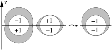
Figure 18: Effective gap of transverse A phase in neutrino processes, shaded area shows the magnitude of the gap.

Let’s look at the order parameter of the A phase:

$$\mathcal{M} = J_{3}\left[\bm{\gamma}_{\perp}^{1}(\widehat{\mathbf{k}})+\bm{\gamma}_{\perp}^{2}(\widehat{\mathbf{k}})\right],$$

where $\bm{\gamma}_{\perp}=\bm{\gamma}-\widehat{\mathbf{k}}\bm{\gamma}\cdot\widehat{\mathbf{k}}$. In the A phase, one direction is chosen to break the color and spin symmetry. This direction is assumed to be along the z-axis. ’1’ and ’2’ are two transverse directions to the z-axis. The excitation branches are characterized by eigenvalues $\lambda_{r}$ of $\mathcal{M}^{\dagger}\mathcal{M}$. Here are excitation energies

$$\epsilon_{r} = \sqrt{(k-\mu)^{2}+\lambda_{r}\phi^{2}},$$

where $\lambda_{r}$ are given by

$$\lambda_{1,2} = (1+|\cos\theta_{k}|^{2})$$

$$\lambda_{3} = 0,$$

where $\theta_{k}$ is the angle between the momentum and the z-axis. So we have spectral representation for $\mathcal{M}^{\dagger}\mathcal{M}$

$$\mathcal{M}^{\dagger}\mathcal{M} = \lambda_{1}\mathcal{P}_{1}+\lambda_{2}\mathcal{P}_{2},$$

where the projectors are

$$\mathcal{P}_{1,2} = \frac{1}{2}J_{3}^{2}\left[1\pm\mathrm{sgn}(\cos\theta_{k})\gamma_{0}\gamma_{5}\bm{\gamma}\cdot\widehat{\mathbf{k}}\right]$$

$$= \frac{1}{2}J_{3}^{2}\left[1\mp\mathrm{sgn}(\cos\theta_{k})\right]H^{+}(\widehat{\mathbf{k}})$$

$$+\frac{1}{2}J_{3}^{2}\left[1\pm\mathrm{sgn}(\cos\theta_{k})\right]H^{-}(\widehat{\mathbf{k}}).$$

Here the helicity projectors are given by:

$$H^{\pm}(\widehat{\mathbf{k}}) = \frac{1}{2}[1\pm\gamma_{5}\gamma_{0}\bm{\gamma}\cdot\widehat{\mathbf{k}}]$$

$$= \frac{1}{2}[1\pm\bm{\Sigma}\cdot\widehat{\mathbf{k}}],$$

where $\bm{\Sigma}=\mathrm{diag}(\sigma,\sigma)$. We see that for the first excitation branch $\lambda_{1}$, the mometum modes with the positive z-component must be negative in helicity, while the modes with negative z-component is positive in helicity. The second excitation branch just shows an opposite helicity correlation. Since the Urca processes involve exchanging W-bosons, only the particles with negative helicity can participate. This fact can be seen by inserting $H^{h}$ with $h=\pm$ into Eq. (212) where the Dirac trace becomes

$$\mathrm{Quark}\;\mathrm{Trace} = \mathrm{Tr}_{s}[\gamma^{\mu}(1-\gamma_{5})\gamma_{0}H^{h_{u}}(\widehat{\mathbf{p}}_{u})\Lambda_{\mathbf{p}_{u}}^{-}$$ (215)

$$\times\gamma^{\nu}(1-\gamma_{5})\gamma_{0}H^{h_{d}}(\widehat{\mathbf{p}}_{d})\Lambda_{\mathbf{p}_{d}}^{-}].$$

We use

$$\bm{\Sigma}\cdot\widehat{\mathbf{p}}\Lambda_{\mathbf{p}}^{-} = -\gamma_{5}\Lambda_{\mathbf{p}}^{-}$$

$$H^{h_{u}}(\widehat{\mathbf{p}})\Lambda_{\mathbf{p}}^{-} = \frac{1}{2}(1-h_{u}\gamma_{5})\Lambda_{\mathbf{p}}^{-}$$

to rewrite the trace (215) as

$$\mathrm{Quark}\;\mathrm{Trace} \sim \mathrm{Tr}_{s}[\gamma^{\mu}(1-\gamma_{5})\gamma_{0}(1-h_{u}\gamma_{5})(\widehat{\mathbf{p}}_{u})\Lambda_{\mathbf{p}_{u}}^{-}$$

$$\times\gamma^{\nu}(1-\gamma_{5})\gamma_{0}(1-h_{d}\gamma_{5})\Lambda_{\mathbf{p}_{d}}^{-}]$$

$$= 0,\;\;\mathrm{for}\;h_{u,d}=+.$$

We see that components with positive helicity $h_{u,d}=+$ vanish. This selects upper part of the first branch and the lower part of the second branch, which gives an effective mode showing asymmetry along the z-direction, see Fig. (18). We know that the larger the gap is, the more suppression the neutrino emission gets. So from the right graph of Fig. (18) we see that the effective gap is larger in the upper half plane (positive z-component) than in the lower one (negative z-component). This means that the neutrino emission along the positive z-axis is more suppressed than in the negative z-axis. This asymmetry can be regarded as an example for parity violation in macroscopic scales.

References

- [1] B. C. Barrois, Nucl. Phys. B 129, 390 (1977).
- [2] D. Bailin and A. Love, Phys. Rept. 107, 325 (1984).
- [3] K. Rajagopal and F. Wilczek, arXiv:hep-ph/0011333.
- [4] M. G. Alford, Ann. Rev. Nucl. Part. Sci. 51, 131 (2001) [arXiv:hep-ph/0102047].
- [5] D. H. Rischke, Prog. Part. Nucl. Phys. 52, 197 (2004) [arXiv:nucl-th/0305030].
- [6] R. Casalbuoni and G. Nardulli, Rev. Mod. Phys. 76, 263 (2004) [arXiv:hep-ph/0305069].
- [7] T. Schafer, arXiv:hep-ph/0304281.
- [8] M. Buballa, Phys. Rept. 407, 205 (2005) [arXiv:hep-ph/0402234].
- [9] H. c. Ren, arXiv:hep-ph/0404074.
- [10] I. A. Shovkovy, Found. Phys. 35, 1309 (2005) [arXiv:nucl-th/0410091].
- [11] M. Huang, Int. J. Mod. Phys. E 14, 675 (2005) [arXiv:hep-ph/0409167].
- [12] A. Gerhold, arXiv:hep-ph/0503279.
- [13] A. Rebhan, arXiv:hep-ph/0504023.
- [14] M. G. Alford, A. Schmitt, K. Rajagopal and T. Schafer, Rev. Mod. Phys. 80, 1455 (2008) [arXiv:0709.4635 [hep-ph]].
- [15] D. J. Gross and F. Wilczek, Phys. Rev. Lett. 30, 1343 (1973).
- [16] H. D. Politzer, Phys. Rev. Lett. 30, 1346 (1973).
- [17] http://nobelprize.org/physics/laureates/2004/gross-lecture.html
- [18] http://nobelprize.org/physics/laureates/2004/wilczek-lecture.html
- [19] M. G. Alford, K. Rajagopal and F. Wilczek, Phys. Lett. B 422, 247 (1998) [arXiv:hep-ph/9711395].
- [20] R. Rapp, T. Schafer, E. V. Shuryak and M. Velkovsky, Phys. Rev. Lett. 81, 53 (1998) [arXiv:hep-ph/9711396].
- [21] S. B. Ruster, I. A. Shovkovy and D. H. Rischke, Nucl. Phys. A 743, 127 (2004) [arXiv:hep-ph/0405170].
- [22] K. Fukushima, C. Kouvaris and K. Rajagopal, Phys. Rev. D 71, 034002 (2005) [arXiv:hep-ph/0408322].
- [23] S. B. Ruster, V. Werth, M. Buballa, I. A. Shovkovy and D. H. Rischke, arXiv:hep-ph/0503184.
- [24] D. Blaschke, S. Fredriksson, H. Grigorian, A. M. Oztas and F. Sandin, arXiv:hep-ph/0503194.
- [25] B. Vanderheyden and A. D. Jackson, Phys. Rev. D 62, 094010 (2000) [arXiv:hep-ph/0003150].
- [26] B. Vanderheyden and A. D. Jackson, Phys. Rev. D 64, 074016 (2001) [arXiv:hep-ph/0102064].
- [27] R. D. Pisarski and D. H. Rischke, Phys. Rev. D 61, 051501 (2000) [arXiv:nucl-th/9907041].
- [28] D. K. Hong, V. A. Miransky, I. A. Shovkovy and L. C. R. Wijewardhana, Phys. Rev. D 61, 056001 (2000) [Erratum-ibid. D 62, 059903 (2000)] [arXiv:hep-ph/9906478].
- [29] T. Schafer, Phys. Rev. D 62, 094007 (2000)[arXiv:hep-ph/0006034].
- [30] A. Schmitt, Q. Wang and D. H. Rischke, Phys. Rev. D 66, 114010 (2002) [arXiv:nucl-th/0209050].
- [31] M. G. Alford, J. A. Bowers, J. M. Cheyne and G. A. Cowan, Phys. Rev. D 67, 054018 (2003) [arXiv:hep-ph/0210106].
- [32] A. Schmitt, Q. Wang and D. H. Rischke, Phys. Rev. Lett. 91, 242301 (2003) [arXiv:nucl-th/0301090].
- [33] A. Schmitt, arXiv:nucl-th/0405076.
- [34] A. Schmitt, Phys. Rev. D 71, 054016 (2005) [arXiv:nucl-th/0412033].
- [35] D. N. Aguilera, D. Blaschke, M. Buballa and V. L. Yudichev, Phys. Rev. D 72, 034008 (2005) [arXiv:hep-ph/0503288].
- [36] T. Brauner, Phys. Rev. D 78, 125027 (2008) [arXiv:0810.3481 [hep-ph]].
- [37] T. Brauner, J. y. Pang and Q. Wang, arXiv:0909.4201 [hep-ph].
- [38] M. Buballa, J. Hosek and M. Oertel, Phys. Rev. Lett. 90, 182002 (2003) [arXiv:hep-ph/0204275].
- [39] M. Huang and I. A. Shovkovy, Phys. Rev. D 70, 051501 (2004) [arXiv:hep-ph/0407049].
- [40] M. Huang and I. A. Shovkovy, Phys. Rev. D 70, 094030 (2004) [arXiv:hep-ph/0408268].
- [41] R. Casalbuoni, R. Gatto, M. Mannarelli, G. Nardulli and M. Ruggieri, Phys. Lett. B 605, 362 (2005) [arXiv:hep-ph/0410401].
- [42] M. Alford and Q. h. Wang, arXiv:hep-ph/0501078.
- [43] M. G. Alford, J. A. Bowers and K. Rajagopal, Phys. Rev. D 63, 074016 (2001) [arXiv:hep-ph/0008208].
- [44] I. Giannakis and H. C. Ren, Phys. Lett. B 611, 137 (2005) [arXiv:hep-ph/0412015].
- [45] I. Giannakis and H. C. Ren, arXiv:hep-th/0504053.
- [46] D. Vollhardt and P. Wölfle, The superfluid phases of Helium 3 (Taylor & Francis, London 1990).
- [47] Y. Nambu and G. Jona-Lasinio, Phys. Rev. 122, 345 (1961).
- [48] J. Goldstone, Nuovo Cim. 19, 154 (1961).
- [49] V. A. Miransky, I. A. Shovkovy and L. C. R. Wijewardhana, Phys. Rev. D 64, 096002 (2001) [arXiv:hep-ph/0104194].
- [50] D. H. Rischke and I. A. Shovkovy, Phys. Rev. D 66, 054019 (2002) [arXiv:nucl-th/0205080].
- [51] V. A. Miransky and I. A. Shovkovy, Phys. Rev. Lett. 88, 111601 (2002) [arXiv:hep-ph/0108178].
- [52] R. Casalbuoni, Z. y. Duan and F. Sannino, Phys. Rev. D 62, 094004 (2000) [arXiv:hep-ph/0004207].
- [53] R. Casalbuoni, Z. Duan and F. Sannino, Phys. Rev. D 63, 114026 (2001) [arXiv:hep-ph/0011394].
- [54] M. G. Alford, J. Berges and K. Rajagopal, Nucl. Phys. B 571, 269 (2000) [arXiv:hep-ph/9910254].
- [55] M. Alford and G. Good, Phys. Rev. D 70, 036008 (2004) [arXiv:hep-ph/0404214].
- [56] E. J. Ferrer, V. de la Incera and C. Manuel, Phys. Rev. Lett. 95, 152002 (2005) [arXiv:hep-ph/0503162].
- [57] E. J. Ferrer, V. de la Incera and C. Manuel, Nucl. Phys. B 747, 88 (2006) [arXiv:hep-ph/0603233].
- [58] E. J. Ferrer and V. de la Incera, Phys. Rev. Lett. 97, 122301 (2006) [arXiv:hep-ph/0604136].
- [59] E. J. Ferrer and V. de la Incera, Phys. Rev. D 76, 045011 (2007) [arXiv:nucl-th/0703034].
- [60] R. Ouyed and F. Sannino, Phys. Lett. B 511, 66 (2001) [arXiv:hep-ph/0103168].
- [61] R. Ouyed and F. Sannino, Astron. Astrophys. 387, 725 (2002) [arXiv:astro-ph/0103022].
- [62] J.M. Cornwall, R. Jackiw, and E. Tomboulis, Phys. Rev. D 10, 2428 (1974).
- [63] H. Kleinert, Fortsch. Phys. 30, 351 (1982).
- [64] A. Gerhold and A. Rebhan, Phys. Rev. D 68, 011502 (2003).
- [65] D.D. Dietrich and D.H. Rischke, Prog. Part. Nucl. Phys. 53, 305 (2004).
- [66] M. Le Bellac, Thermal Field Theory (Cambridge, Cambridge University Press, 1996).
- [67] W. E. Brown, J. T. Liu and H. c. Ren, Phys. Rev. D 62, 054013 (2000) [arXiv:hep-ph/0003199].
- [68] Q. Wang and D. H. Rischke, Phys. Rev. D 65, 054005 (2002) [arXiv:nucl-th/0110016].
- [69] T. Schafer and K. Schwenzer, Phys. Rev. D 70, 054007 (2004) [arXiv:hep-ph/0405053].
- [70] A. Gerhold and A. Rebhan, Phys. Rev. D 71, 085010 (2005) [arXiv:hep-ph/0501089].
- [71] C. Manuel, Phys. Rev. D 62, 114008 (2000).
- [72] D. T. Son, Phys. Rev. D 59, 094019 (1999) [arXiv:hep-ph/9812287].
- [73] R. D. Pisarski and D. H. Rischke, Phys. Rev. D 61, 074017 (2000) [arXiv:nucl-th/9910056].
- [74] T. Schafer and F. Wilczek, Phys. Rev. D 60, 114033 (1999) [arXiv:hep-ph/9906512].
- [75] A.L. Fetter and J.D. Walecka, Quantum Theory of Many Particle Systems (McGraw-Hill, New York, 1971).
- [76] M. Kitazawa, T. Koide, T. Kunihiro and Y. Nemoto, Phys. Rev. D 70, 056003 (2004) [arXiv:hep-ph/0309026].
- [77] M. Kitazawa, T. Koide, T. Kunihiro and Y. Nemoto, arXiv:hep-ph/0502035.
- [78] I. Giannakis, D. f. Hou, H. c. Ren and D. H. Rischke, Phys. Rev. Lett. 93, 232301 (2004) [arXiv:hep-ph/0406031].
- [79] D. f. Hou, Q. Wang and D. H. Rischke, Phys. Rev. D 69, 071501 (2004) [arXiv:hep-ph/0401152].
- [80] H. j. Xu and Q. Wang, Chin. Phys. C 33, 753 (2009) [arXiv:0810.2168 [hep-ph]].
- [81] D. Nickel, J. Wambach and R. Alkofer, Phys. Rev. D 73, 114028 (2006) [arXiv:hep-ph/0603163].
- [82] F. Marhauser, D. Nickel, M. Buballa and J. Wambach, Phys. Rev. D 75, 054022 (2007) [arXiv:hep-ph/0612027].
- [83] D. H. Rischke, Phys. Rev. D 64, 094003 (2001) [arXiv:nucl-th/0103050].
- [84] H. Malekzadeh and D. H. Rischke, Phys. Rev. D 73, 114006 (2006) [arXiv:hep-ph/0602082].
- [85] H. Malekzadeh, Phys. Rev. D 79, 034010 (2009) [arXiv:0810.5235 [hep-ph]].
- [86] A. Schmitt, Q. Wang and D. H. Rischke, Phys. Rev. D 69 (2004) 094017 [arXiv:nucl-th/0311006].
- [87] D. H. Rischke, Phys. Rev. D 62, 034007 (2000) [arXiv:nucl-th/0001040].
- [88] C. Manuel and K. Rajagopal, Phys. Rev. Lett. 88, 042003 (2002) [arXiv:hep-ph/0107211].
- [89] D. F. Litim and C. Manuel, Phys. Rev. D 64, 094013 (2001) [arXiv:hep-ph/0105165].
- [90] K. Iida and G. Baym, Phys. Rev. D 63, 074018 (2001) [Erratum-ibid. D 66, 059903 (2002)] [arXiv:hep-ph/0011229].
- [91] K. Iida and G. Baym, Phys. Rev. D 65, 014022 (2002) [arXiv:hep-ph/0108149].
- [92] K. Iida and G. Baym, Phys. Rev. D 66, 014015 (2002) [arXiv:hep-ph/0204124].
- [93] I. Giannakis and H. c. Ren, Phys. Rev. D 65, 054017 (2002) [arXiv:hep-ph/0108256].
- [94] I. Giannakis and H. c. Ren, Nucl. Phys. B 669, 462 (2003) [arXiv:hep-ph/0305235].
- [95] D. Blaschke, D. M. Sedrakian and K. M. Shahabasian, Astron. Astrophys. 350, L47 (1999) [arXiv:astro-ph/9904395].
- [96] D. M. Sedrakian, D. Blaschke, K. M. Shahabasyan and D. N. Voskresensky, Astrofiz. 44, 443 (2001) [arXiv:hep-ph/0012383].
- [97] D. K. Hong, Phys. Lett. B 473, 118 (2000) [arXiv:hep-ph/9812510].
- [98] T. Schafer, Nucl. Phys. A 728, 251 (2003) [arXiv:hep-ph/0307074].
- [99] T. Schafer, arXiv:hep-ph/0402032.
- [100] G. Nardulli, Riv. Nuovo Cim. 25N3, 1 (2002) [arXiv:hep-ph/0202037].
- [101] P. T. Reuter, Q. Wang and D. H. Rischke, Phys. Rev. D 70, 114029 (2004) [arXiv:nucl-th/0405079].
- [102] P. T. Reuter, Q. Wang and D. H. Rischke, arXiv:nucl-th/0409051.
- [103] T. Schafer and F. Wilczek, Phys. Lett. B 450, 325 (1999) [arXiv:hep-ph/9810509].
- [104] R. D. Pisarski and D. H. Rischke, Phys. Rev. D 60, 094013 (1999) [arXiv:nucl-th/9903023].
- [105] T. Hatsuda and T. Kunihiro, Phys. Rept. 247, 221 (1994) [arXiv:hep-ph/9401310].
- [106] Y. Nishida and H. Abuki, Phys. Rev. D 72, 096004 (2005) [arXiv:hep-ph/0504083].
- [107] H. Abuki, Nucl. Phys. A 791, 117 (2007) [arXiv:hep-ph/0605081].
- [108] M. Kitazawa, D. H. Rischke and I. A. Shovkovy, Prog. Theor. Phys. Suppl. 168, 389 (2007) [arXiv:0707.3966 [nucl-th]].
- [109] M. Kitazawa, D. H. Rischke and I. A. Shovkovy, Phys. Lett. B 663, 228 (2008) [arXiv:0709.2235 [hep-ph]].
- [110] G. f. Sun, L. He and P. Zhuang, Phys. Rev. D 75, 096004 (2007) [arXiv:hep-ph/0703159].
- [111] L. He and P. Zhuang, Phys. Rev. D 76, 056003 (2007) [arXiv:0705.1634 [hep-ph]].
- [112] T. Brauner, Phys. Rev. D 77, 096006 (2008) [arXiv:0803.2422 [hep-ph]].
- [113] D. Blaschke and D. Zablocki, Phys. Part. Nucl. 39, 1010 (2008) [arXiv:0812.0589 [hep-ph]].
- [114] R. Friedberg and T. D. Lee, Phys. Rev. B 40, 6745 (1989).
- [115] J. Deng, A. Schmitt and Q. Wang, Phys. Rev. D 76, 034013 (2007) [arXiv:nucl-th/0611097].
- [116] J. Deng, J. c. Wang and Q. Wang, Phys. Rev. D 78, 034014 (2008) [arXiv:0803.4360 [hep-ph]].
- [117] S. Y. Chang, V. R. Pandharipande, J. Carlson and K. E. Schmidt, Phys. Rev. A 70, 043602 (2004) [arXiv:physics/0404115].
- [118] J. Carlson and S. Reddy, Phys. Rev. Lett. 95, 060401 (2005) [arXiv:cond-mat/0503256].
- [119] Y. Nishida and D. T. Son, Phys. Rev. Lett. 97, 050403 (2006) [arXiv:cond-mat/0604500].
- [120] I. Shovkovy and M. Huang, Phys. Lett. B 564, 205 (2003) [arXiv:hep-ph/0302142].
- [121] E. Gubankova, A. Schmitt and F. Wilczek, Phys. Rev. B 74, 064505 (2006) [arXiv:cond-mat/0603603].
- [122] K. Rajagopal and A. Schmitt, Phys. Rev. D 73, 045003 (2006) [arXiv:hep-ph/0512043].
- [123] S. Tsuruta and A.G.W. Cameron, Canad. J. Phys. 44, 1863(1966).
- [124] D. G. Yakovlev and C. J. Pethick, Ann. Rev. Astron. Astrophys. 42, 169 (2004) [arXiv:astro-ph/0402143].
- [125] M. Prakash, J. M. Lattimer, J. A. Pons, A. W. Steiner and S. Reddy, Lect. Notes Phys. 578, 364 (2001) [arXiv:astro-ph/0012136].
- [126] D. Blaschke, H. Grigorian and D. N. Voskresensky, Astron. Astrophys. 424, 979 (2004) [arXiv:astro-ph/0403170].
- [127] N. Iwamoto, Phys. Rev. Lett. 44, 1637 (1980).
- [128] T. Schafer and K. Schwenzer, Phys. Rev. D 70, 114037 (2004) [arXiv:astro-ph/0410395].
- [129] A. Ipp, A. Gerhold and A. Rebhan, Phys. Rev. D 69, 011901 (2004) [arXiv:hep-ph/0309019].
- [130] A. Gerhold, A. Ipp and A. Rebhan, Phys. Rev. D 70, 105015 (2004) [arXiv:hep-ph/0406087].
- [131] D. Blaschke, T. Klahn and D. N. Voskresensky, Astrophys. J. 533, 406 (2000) [arXiv:astro-ph/9908334].
- [132] D. Page, M. Prakash, J. M. Lattimer and A. Steiner, Phys. Rev. Lett. 85, 2048 (2000) [arXiv:hep-ph/0005094].
- [133] A. Schmitt, I. A. Shovkovy and Q. Wang, Phys. Rev. D 73, 034012 (2006) [arXiv:hep-ph/0510347].
- [134] Q. Wang, Z. g. Wang and J. Wu, Phys. Rev. D 74, 014021 (2006) [arXiv:hep-ph/0605092].
- [135] P. Jaikumar, M. Prakash and T. Schafer, Phys. Rev. D 66, 063003 (2002) [arXiv:astro-ph/0203088].
- [136] P. Jaikumar and M. Prakash, Phys. Lett. B 516, 345 (2001) [arXiv:astro-ph/0105225].
- [137] J. Kundu and S. Reddy, Phys. Rev. C 70, 055803 (2004) [arXiv:nucl-th/0405055].
- [138] M. Alford, P. Jotwani, C. Kouvaris, J. Kundu and K. Rajagopal, Phys. Rev. D 71, 114011 (2005) [arXiv:astro-ph/0411560].
- [139] P. Jaikumar, C. D. Roberts and A. Sedrakian, Phys. Rev. C 73, 042801 (2006) [arXiv:nucl-th/0509093].
- [140] X. g. Huang, Q. Wang and P. f. Zhuang, Phys. Rev. D 76, 094008 (2007) [arXiv:0706.4381 [hep-ph]].
- [141] X. g. Huang, Q. Wang and P. f. Zhuang, Int. J. Mod. Phys. E 17, 1906 (2008) [arXiv:0710.3634 [hep-ph]].
- [142] Q. Wang, K. Redlich, H. Stocker and W. Greiner, Phys. Rev. Lett. 88, 132303 (2002) [arXiv:nucl-th/0111040].
- [143] Q. Wang, K. Redlich, H. Stocker and W. Greiner, Nucl. Phys. A 714, 293 (2003) [arXiv:hep-ph/0202165].
- [144] A. Sedrakian and A. Dieperink, Phys. Lett. B 463, 145 (1999) [arXiv:nucl-th/9905039].
- [145] A. Sedrakian and A. E. L. Dieperink, Phys. Rev. D 62, 083002 (2000) [arXiv:astro-ph/0002228].
- [146] D. H. Rischke, Phys. Rev. D 62, 054017 (2000) [arXiv:nucl-th/0003063].
- [147] Q. Wang, AIP Conf. Proc. 865, 248 (2006) [arXiv:hep-ph/0607096].
- [148] D. Blaschke, F. Sandin and T. Klahn, J. Phys. G 35, 104077 (2008) [arXiv:0808.0181 [nucl-th]].
- [149] D. Blaschke, F. Sandin, T. Klahn and J. Berdermann, AIP Conf. Proc. 1038, 183 (2008) [arXiv:0808.1369 [astro-ph]].
- [150] A. Schmitt, I. A. Shovkovy and Q. Wang, Phys. Rev. Lett. 94, 211101 (2005); Erratum: Phys. Rev. Lett. 95, 159902 (2005) [arXiv:hep-ph/0502166].