Edge States and Quantum Hall Effect in Graphene under a Modulated Magnetic Field

Abstract

Graphene properties can be manipulated by a periodic potential. Based on the tight-binding model, we study graphene under a one-dimensional (1D) modulated magnetic field which contains both a uniform and a staggered component. The chiral current-carrying edge states generated at the interfaces where the staggered component changes direction, lead to an unusual integer quantum Hall effect (QHE) in graphene, which can be observed experimentally by a standard four-terminal Hall measurement. When Zeeman spin splitting is considered, a novel state is predicted where the electron edge currents with opposite polarization propagate in the opposite directions at one sample boundary, whereas propagate in the same directions at the other sample boundary.

Recently, graphene materials have received extensive theoretical and experimental studiesCastro Neto2009 . The most important physical properties of graphene are governed by the underlying chiral Dirac fermionsZhou2006 ; Li2007 . These Dirac fermions under a uniform magnetic field (UMF) give rise to the well-known anomalous QHENovoselov2005 ; Zhang2005 , which has been experimentally verified and is now believed to be a unique feature to characterize graphene. Spin QHE was also predicted in graphene, where electron edge current with the opposite spin polarization couterpropagates due to the spin-orbit interactionKane2005 or the Zeeman spin splitting of the zeroth Landau level (LL)Abanin2006 . On the other hand, the experimental manipulation of the electronic structure of graphene has potential application in graphene electronics or spintronicsRycerz2007 ; Son2006 . One method to manipulate the physical properties of graphene is by applying periodic electronicPark2008 ; Park2009 or magnetic potentialsDellAnna2009 ; DellAnna2009-2 , which can be realized now by making use of substrateVazquez2008 ; Martoccia2008 ; Sutter2008 ; Pletikosic2009 or controlled adatom depositionMeyer2008 .

Here, we report the investigation of the effect on graphene QHE of a 1D staggered magnetic field (SMF), which is schematically shown in the top panels of Fig. 1. The 1D SMF can be achieved in experiments by applying an array of ferromagnetic stripes with alternative magnetization on the top of a graphene layer. It is found that the edge states created by 1D SMF lead to a nontrivial robust integer QHE in graphene. In a standard four-terminal Hall measurement, when varying the magnitude of the UMF, graphene can undergo a transition from a state with unusual quantized Hall conductance to one without Hall effect. Furthermore, the Zeeman spin splitting of the zeroth LL of graphene gives rise to a novel state where spin-up and spin-down edge currents have the opposite chirality at one sample boundary but have the same chirality at the other sample boundary.

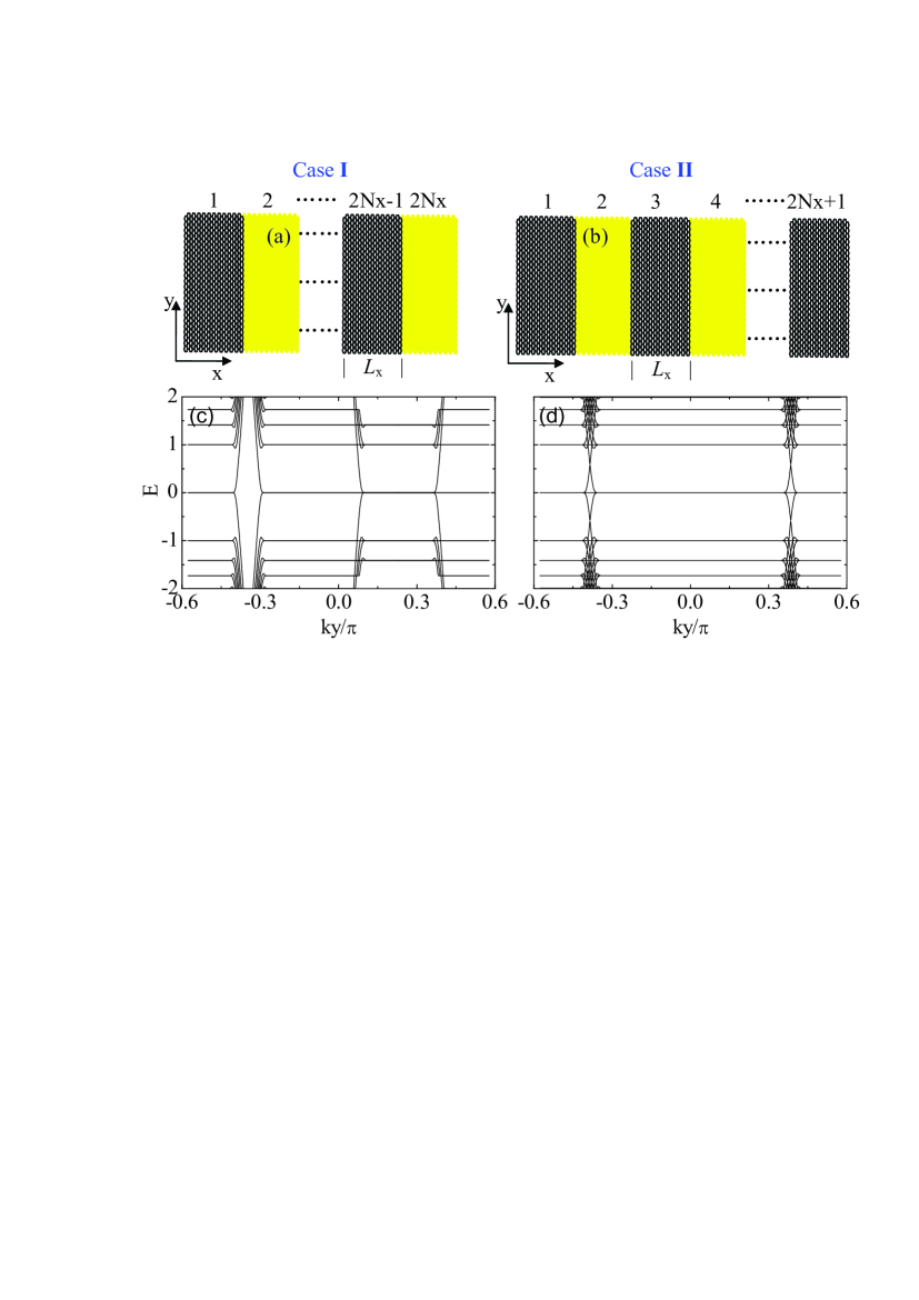
Figure 1: (color online). Top panels: Schematic illustration of a rectangular graphene sample under a SMF, where two uniform fields which are the same in magnitudes but opposite in directions alternate every $Lx$ distance. Case I in (a) contains $2N_{x}$ alternating regions whereas Case II in (b) contains $2N_{x}+1$ alternating regions, with $N_{x}$ an integer. Bottom panels: Electron energy bands of graphene under a periodically SMF with $L_{x}=426$ nm, and $B_{S}=24$ T for (c), $B_{S}=40$ T for (d). Energy is measured in unit of $\hbar v_{F}/l_{B}$ with $l_{B}$ the magnetic length. For the parameters chosen, $l_{B}$ is determined to be $l_{B}=3.7$ nm for (c), $l_{B}=2.9$ nm for (d), respectively.

We start from the tight-binding model on a honeycomb lattice in a perpendicular nonuniform magnetic field described by the Hamiltonian,

$$H=-t\sum_{<ij>}e^{i\int_{i}^{j}\textbf{A}\cdot d\textbf{l}}c_{i}^{\dagger}c_{j}+\texttt{H.c.},$$ (1)

where $t$ is the hopping integral, the operator $c_{i}^{\dagger}$ ($c_{i}$) creates (annihilates) an electron at site $i$, and $<ij>$ denotes nearest-neighbor pairs of sites. A is the gauge potential for the nonuniform magnetic field. The Zeeman spin splitting is neglected now for simplicity and will be discussed later. We distinguish here Case I in Fig. 1(a) from Case II in Fig. 1(b) because graphene in Case I has no QHE unless the magnetic fields of the two alternating areas have the same directions, i.e. $B_{U}>B_{S}$ where $B_{U}$ and $B_{S}$ are the magnitudes of the UMF and SMF respectively. The reason for this will be explained later when we discuss Fig. 2.

The LLs of grapheneMcClure1956 can be expressed as $E_{n}=\pm\hbar v_{F}\sqrt{|n|}/l_{B}$ with $l_{B}=\sqrt{\hbar c/2eB}$ the magnetic length, $v_{F}=3at/2\hbar$ the Fermi velocity, and $n=0,1,2,...$ the LL index. Here $a$ is graphene lattice constant. The physical picture at large $L_{x}$ order of $L_{x}>>l_{B}$ is found to be quite different from that at smaller $L_{x}$ case with $L_{x}\sim l_{B}$, where only a few chains are contained in each alternating area. In the latter case, though Dirac cone structure is preserved, more and more Dirac points are created as increasing $L_{x}$Xu , and finally the LLs of graphene appear. In Figs. 1(c) and 1(d) we show in the absence of the UMF the electron energy bands of graphene under a periodic SMF with $k_{x}=0$. For the SMF with a period $2L_{x}$, we have chosen correspondingly a periodic gauge $\textbf{A}=\textbf{A}_{S}=(0,B_{S}|x|,0)$ for $|x|<L_{x}$. When energy is set by $\hbar v_{F}/l_{B}$, the $\sqrt{n}$ spacing of the LLs of graphene can be seen clearly. What’s remarkable is that for large $L_{x}$, the dense Dirac points are emerged into the zeroth LL of grapheneXu . Compared with the LLs of graphene in a UMF, which is dispersionless, the energy bands have non-flat regions where energy disperse with $k_{y}$, indicating the presence of edge states. These new edge states which were called magnetic edge statesReijniers2001 ; Sim1998 are actually generated by the SMF and right located at the interfaces where the SMF changes direction, providing the gapless excitations for even an infinite graphene.

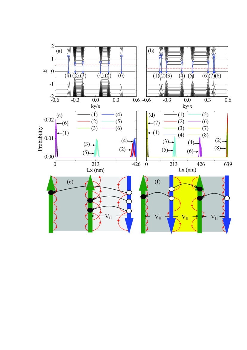
Figure 2: (color online). Top panels: Electron energy spectrum of graphene in the presence of both a UMF and a SMF for $N_{x}=1$ and $L_{x}=213$ nm. (a) belongs to Case I with parameters $B_{U}=24$ T, $B_{S}=16$ T. (b) belongs to Case II with parameters $B_{U}=16$ T, $B_{S}=32$ T. Here energy is scaled in the same way to Fig. 1 except the magnetic length $l_{B}$ is replaced by that for the high-field regions. The red dashed lines represent the positions of the chemical potentials. Middle panels: The corresponding electron probability densities for the representative states indicated in the top panels by the open circles. Bottom panels: Schematic diagrams of the corresponding electron edge currents (green and blue arrows) and electrons’ classical skipping orbits. $V_{H}$ is the Hall voltage. Gray (light gray, yellow) solid rectangle represents high-(low-) field regions. Black and white solid circles represent particle-hole excitations in the Laughlin’s thought experiment.

To further clarify the physical properties of these edge states and its consequences, we study the QHE of such a system, i.e., the graphene samples in the presence of both a UMF and a SMF. In the following cases, open boundary condition is applied in the $x$ direction and periodic boundary condition in the $y$ direction, and the Landau gauge $\textbf{A}_{U}=(0,B_{U}x,0)$ is adopted for the UMF and $\textbf{A}=\textbf{A}_{S}+\textbf{A}_{U}$. The graphene energy spectrum for Case I and Case II are calculated and shown in Figs. 2(a) and 2(b), respectively. With application of a UMF, the graphene samples can be divided into two groups of regions, where one is the high-field group of regions with the magnetic field $B_{U}+B_{S}$, the other is the low-field group of regions with the magnetic field $B_{U}-B_{S}$. Correspondingly, the bulk excitations of the graphene system have two groups of LLs, which are reflected in electron energy bands by the two groups of the flat regions in Figs. 2(a) and 2(b). Interestingly, when the ratio $(B_{U}-B_{S})/(B_{U}+B_{S})=p/q$, where $p$ and $q$ are two coprime integers, a series of LLs will be doubly degenerate, which may cause some interesting phenomena. In particular, we actually have $(B_{U}-B_{S})/(B_{U}+B_{S})=1/5$ and $-1/3$ for the parameters in Figs. 2(a) and 2(b), respectively, resulting in the doubly degeneracy of all the LLs in the high-field regions.

Now we focus our attention on the edge states. In Figs. 2(c) and 2(d), electron probability densities for representative edge states are shown. Except the conventional edge states located at the sample boundaries [see (1),(2),(4),(6) in Fig. 2(c), and (1),(2),(7),(8) in Fig. 2(d)], new edge states are generated and right localized at the interfaces where the SMF changes direction [see (3),(5) in Fig. 2(c), and (3)-(6) in Fig. 2(d)]. Clearly, these edge states are also chiral current-carrying statess-Park2008 ; Oroszlany2008 ; Ghosh2008 , whose flowing directions can be easily determined by the slopes of the bands where they are located. All the edge currents are schematically shown in the bottom panels of Fig. 2. Also indicated in these panels are the classical orbits of electronsMuller1992 , which are composed of arcs with the length scale approximately equal to the magnetic length $l_{B}$. These classical orbits give a simple physical interpretation of the reason why the edge currents flow in the shown directions.

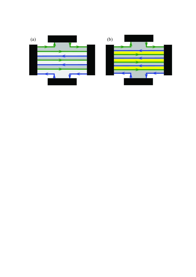
Figure 3: (color online). The four-terminal Hall bar geometries for (a) Case I and (b) Case II with $N_{x}=3$. The black solid rectangles represent contacts and the lines with arrows represent the edge currents.

Let us now consider the corresponding four-terminal Hall measurements. Assuming that contacts are reflectionless, all edge currents coming from the same contact share the same voltage with that contact, so that all the “ up-flowing ” edge currents have the same voltage and so do all the “ down-flowing ” edge currents. The voltage difference between the edge currents with opposite directions is equivalent to the Hall voltage $V_{H}$ between the sample boundaries. To obtain the Hall conductance in these two situations in Figs. 2(e)-(f), we follow Laughlin’s argumentLaughlin1981 and imagine rolling up the graphene ribbon along the $y$ direction to make a graphene cylinder which is then threaded by a magnetic flux. When varying adiabatically the magnetic flux through the graphene cylinder by a flux quantum $\phi_{0}$, particle-hole excitations will be generated both at the sample boundaries and the interfaces where the SMF changes direction. For an illustration, we show schematically in Figs. 2(e)-(f) these excitations for the chemical potentials indicated by the red lines in Figs. 2(a)-(b). The increase in energy due to electrons transfer between the Hall voltage is $\delta E=3eV_{H}$ for both Figs. 2(e) and 2(f). Generally, if the system has such a Fermi energy that the $M$th LL of the high-field regions and the $N$th LL of the Low-field regions are just completely filled, detailed analysis of the edge states in the energy bands shows that the increase in energy $\delta E$ can be given by $\delta E=P_{N}eV_{H}$ for Case I in Fig. 2(e), and $\delta E=(P_{N}+2P_{M})eV_{H}$ for Case II in Fig. 2(f), respectively, where $P_{M}=2M+1$ and $P_{N}=2N+1$. Hence, from $I=c\delta E/\delta\phi$, the Hall conductance is given by $\sigma_{xy}=P_{N}e^{2}/h$ for Case I in Fig. 2(e), which has nothing to do with the high-field LLs, and $\sigma_{xy}=(P_{N}+2P_{M})e^{2}/h$ for Case II in Fig. 2(f).

We note that in order to have the mentioned QHE for Case I(II), the magnetic field for the high-field and low-field regions must have the same (opposite) direction, i.e., $B_{U}>B_{S}$ ($B_{U}<B_{S}$). For Case I in Fig. 2(e), by varying the UMF so that the magnetic field for the low-field region is reversed, i.e., $B_{U}<B_{S}$, the electron edge currents at the right edge and the interface will be reversed too, resulting in the same voltage shared by the two sample boundaries and thus a zero Hall voltage. For Case II in Fig. 2(f), however, the reversal of the magnetic field in the low-field region for $B_{U}>B_{S}$ only leads to the reversal of edge currents at the two interfaces with that at the two sample boundaries unchanged, giving rise to another quantized Hall conductance $\sigma_{xy}=P_{N}e^{2}/h$. Therefore, for both cases, $B_{U}=B_{S}$ is a critical value for graphene QHE under a SMF. Another important point we should remark is that for Case II in Fig. 2(e), even in the absence of a UMF, graphene under a purely SMF shows a quantized Hall conductance $\sigma_{xy}=3P_{N}e^{2}/h$, where $P_{N}=P_{M}$. This can be comparable with the Haldane model introduced in Ref. [Haldane1988, ], where there exists a nonzero quantized Hall conductance in the absence of an external UMF. All these peculiar behaviors are believed to have great application in graphene manipulation.

It is straightforward to generalize the scheme used above to more general and interesting cases for $N_{x}>1$. Our detailed calculation confirm the existence of the two groups of the LLs for both Cases, which are the bulk excitations of graphene under the modulated magnetic field and are represented by the flat bands in the electron spectrum. Except the LLs and conventional edge states at the sample boundaries, there exist many current-carrying edge states localized at the interfaces where the SMF changes direction. In Fig. 3, we take $N_{x}=3$ for example, and show schematically the corresponding four-terminal measurements, where $N_{x}$ now has the meaning of the number of the low-field regions. Detailed analysis of these edge states from the spectrum and similar argument lead to the Hall conductance as follows:

when $B_{U}>B_{S}$, for both Case I and II,

$$\sigma_{xy}^{\text{{I}}}=\sigma_{xy}^{\text{{II}}}=\pm\frac{e^{2}}{h}[N_{x}P_{N}-(N_{x}-1)P_{M}],$$ (2)

when $B_{U}<B_{S}$, for Case II,

$$\sigma_{xy}^{\text{{II}}}=\pm\frac{e^{2}}{h}[N_{x}P_{N}+(N_{x}+1)P_{M}],$$ (3)

whereas for Case I, there is no Hall voltage. Here the “$\pm$” symbol represents the particle-hole symmetry. If $N_{x}=1$, the previous results are recovered. The result Eq. (3) seems trivial since it can be seen as the conductance sum of all the contributions from each distinct region. The result Eq. (2), however, is highly nontrivial since it can not be seen as the naive subtraction of the contribution of the high-field regions from that of the low-field regions. When the chemical potential is within a gap between the LLs, while the Hall conductance is quantized, the resistance of system should be vanishingly small because only the edge states carry current so that the backscattering is strongly suppressed. Due to the gauge invariance of Laughlin’s argument used here, the results we obtained should be robust against weak disorder and interaction. On the other hand, by varying the magnitude of the UMF, we come to a similar conclusion to the cases with $N_{x}=1$ that, the graphene will undergo a transition, from one state with the quantized Hall conductance Eq. (2) to one without Hall effect for Case I in Fig. 3(a), whereas from one state with the Hall conductance Eq. (3) to one with the Hall conductance Eq. (2) for Case II in Fig. 3(b).

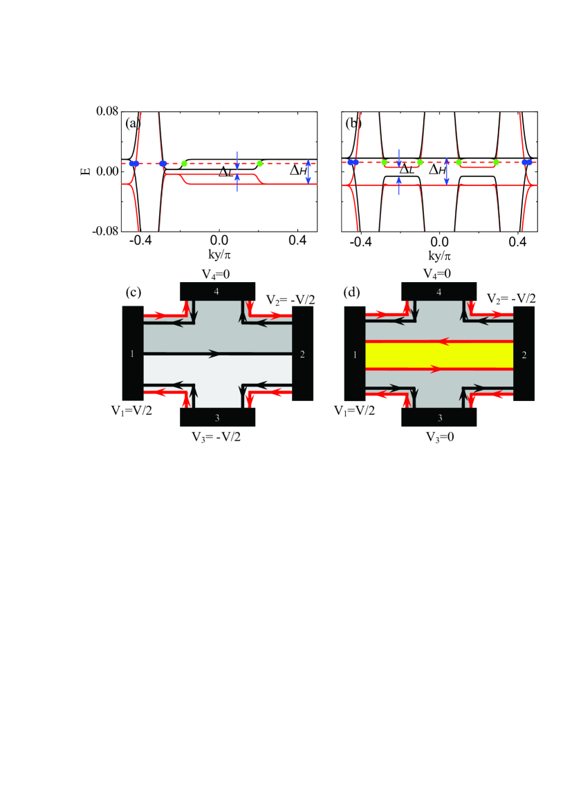
Figure 4: (color online). Top panels: Electron energy spectrum of graphene in the presence of Zeeman splitting for (a) Case I and (b) Case II with $N_{x}=1$. The Zeeman energy is chosen to be one tenth of the largest LL spacing of the high-field regions. The red dashed lines represent the positions of the chemical potentials. The blue filled circles indicate the edge states at the sample boundaries whereas the green filled circles indicate the newly generated edge states localized at the interfaces where the SMF changes direction. Bottom panels: The corresponding four-terminal Hall bar geometries, where the red and black lines with arrows represent the spin-up and spin-down edge currents, respectively.

Now we turn to explore the spin effect in graphene QHE in the presence of Zeeman spin splitting. The energy spectrum is shown in Figs. 4(a)-(b). Two spin gaps $\Delta_{H}$ and $\Delta_{L}$, which are corresponding to the Zeeman splitting in the high-field and low-field regions respectively, are opened. When the chemical potential lies within the interval $-\Delta_{L}/2<\mu<\Delta_{L}/2$, there is no edge current at the interfaces where the SMF changes direction, as well as two edge states at both sample boundaries, which have opposite spin polarizations and propagate in opposite directionsAbanin2006 .

When the chemical potential lies within the interval $\Delta_{L}/2<|\mu|<\Delta_{H}/2$, fully spin-polarized edge currents appear at the interfaces where the SMF changes direction (See the four-terminal Hall measurements shown in Figs. 4(c)-(d)), which is spin-down for $B_{U}>B_{S}$, and spin-up for $B_{U}<B_{S}$. Remarkably, for Case I in Fig. 4(c), a novel state occurs where at one sample boundary spin-up and spin-down currents counterpropagate whereas at the other sample boundary spin-up and spin-down currents propagate in the same directions. Using Landauer conductance formula for the four-terminal geometries we find that for Case I in Fig. 4(c) with a general $N_{x}$, there is spin-polarized charge current $(2N_{x}+1/2)Ve^{2}/h$ flowing from terminal 1 to terminal 2 with a Hall voltage $V/2$, leading to a Hall conductance $\sigma_{xy}=(4N_{x}+1)e^{2}/h$. We note that this feature differs this state from the state of topological insulator since the Hall voltage in the latter state is $0$Abanin2006 , not $V/2$. For Case II in Fig. 4(d) with a general $N_{x}$, there is also a spin-polarized charge current $(2N_{x}+1)Ve^{2}/h$ flowing from terminal 1 to terminal 2 but without a Hall voltage, leading to a resistance $1/\sigma_{xx}=h/(2N_{x}+1)e^{2}$. Interestingly, for Case I in Fig. 4(c), there exist spin currents $(2N_{x}-3/2)Ve^{2}/h$ flowing from terminal 1 and $Ve^{2}/h$ flowing from terminal 4, as well as a spin current $(2N_{x}-1/2)Ve^{2}/h$ flowing to terminal 2, whereas for Case II in Fig. 4(d), there exist a spin current $2N_{x}Ve^{2}/h$ flowing from terminal 2 to terminal 1, as well as a $N_{x}$ independent spin current $Ve^{2}/h$ flowing from terminal 3 to terminal 4. We note that a wave-vector-dependent spin-filtering effect was also revealed recently by a calculation on the transport problem through magnetic barriers in graphene with Zeemann splittingDellAnna2009-2 .

A natural question is that the SMF we considered here is ideal and changes direction abruptly, while in real conditions there exists a length scale $l$ which is the distance covered by the SMF to change direction. Detailed calculation shows that if $l$ is much less than the magnetic length $l_{B}$, our results will be independent of $l$. The $l$ is estimated to be $1$ nm, while for a typical magnetic field order of $10$ T, $l_{B}\sim 10$ nm, satisfying the criterion.

In conclusion, graphene QHE under a modulated orbital magnetic field has been investigated. The current-carrying edge states created by the modulated magnetic field give rise to a novel quantized Hall conductance, which can be checked by a standard four-terminal Hall measurement. By varying the UMF, the four-terminal graphene sample is expected to undergo a transition from a state with novel QHE to one without Hall effect. The effect of Zeeman spin splitting is also discussed and a novel state and its corresponding spin Hall currents are predicted.

- (1) A. H. Castro Neto et al., Rev. Mod. Phys. 81, 109 (2009).
- (2) S. Y. Zhou et al., Nature Phys. 2, 595 (2006)
- (3) G. H. Li, and E. V. Andrei, Nature Phys. 3, 623 (2007).
- (4) K. S. Novoselov et al., Nature (London) 438, 197 (2005).
- (5) Y. Zhang et al., Nature (London) 438, 201 (2005).
- (6) C. L. Kane, and E. J. Mele, Phys. Rev. Lett. 95, 146802 (2005); 95, 226801 (2005).
- (7) D. A. Abanin et al., Phys. Rev. Lett. 96, 176803 (2006).
- (8) A. Rycerz et al., Nature Phys. 3, 172 (2007).
- (9) Y.-W. Son et al., Nature (London) 444, 347 (2006).
- (10) C.-H. Park et al., Nature Phys. 4, 213 (2008); Phys. Rev. Lett. 101, 126804 (2008).
- (11) C.-H. Park et al., Phys. Rev. Lett. 103, 046808 (2009).
- (12) L. Dell’Anna et al., Phys. Rev. B 79, 045420 (2009).
- (13) L. Dell’Anna et al., Phys. Rev. B 80, 155416 (2009).
- (14) A. L. Vázquez de Parga et al., Phys. Rev. Lett. 100, 056807 (2008).
- (15) D. Martoccia et al., Phys. Rev. Lett. 101, 126102 (2008).
- (16) P. W. Sutter et al., Nature Mater. 7, 406 (2008).
- (17) I. Pletikosić et al., Phys. Rev. Lett. 102, 056808 (2009).
- (18) J. C. Meyer et al., Appl. Phys. Lett. 92, 123110 (2008).
- (19) J. W. McClure, Phys. Rev. 104, 666 (1956).
- (20) L. Xu, J. An, and C.-D. Gong, arXiv:0912.4104.
- (21) J. Reijniers et al., Phys. Rev. B 63, 165317 (2001).
- (22) H.-S. Sim et al., Phys. Rev. Lett. 80, 1501 (1998).
- (23) S. Park, and H.-S. Sim, Phys. Rev. B 77, 075433 (2008).
- (24) L. Oroszlány et al., Phys. Rev. B 77, 081403(R) (2008).
- (25) T. K. Ghosh et al., Phys. Rev. B 77, 081404(R) (2008).
- (26) J. E. Müller, Phys. Rev. Lett. 68, 385 (1992).
- (27) R. B. Laughlin, Phys. Rev. B 23, 5632 (1981).
- (28) F. D. M. Haldane, Phys. Rev. Lett. 61, 2015 (1988).