Four highly luminous massive star forming regions in the Norma Spiral Arm.

I. Molecular gas and dust observations

Abstract

We report molecular line and dust continuum observations, made with the SEST telescope, towards four young high-mass star forming regions associated with highly luminous (${\cal L}>6\times 10^{5}{\cal L}_{\odot}$) IRAS sources (15290-5546, 15502-5302, 15567-5236 and 16060-5146). Molecular emission was mapped in three lines of CS (J=2$\rightarrow$1, 3$\rightarrow$2 and 5$\rightarrow$4), two lines of SiO (J=2$\rightarrow$1 and 3$\rightarrow$2), two rotational transitions of CH₃OH (J_k=3${}_{k}\rightarrow 2_{k}$ and $2_{k}\rightarrow 1_{k}$), and in the C³⁴S(J=3$\rightarrow$2) line. In addition, single spectra at the peak position were taken in the CO(J=1$\rightarrow$0), ¹³CO(J=1$\rightarrow$0) and C¹⁸O(J=1$\rightarrow$0) lines. We find that the luminous star forming regions are associated with molecular gas and dust structures with radii of typically 0.5 pc, masses of $\sim 5\times 10^{3}$ M_⊙, column densities of $\sim 5\times 10^{23}$ cm^-2, molecular hydrogen densities of typically $\sim 2\times 10^{5}$ cm^-3 and dust temperatures of $\sim 40$ K. The 1.2 mm dust continuum observations further indicate that the cores are centrally condensed, having radial density profiles with power-law indices in the range $1.6-1.9$. We find that under these conditions dynamical friction by the gas plays an important role in the migration of high-mass stars towards the central core region, providing an explanation for the observed stellar mass segregation within the cores.

The CS profiles show two distinct emission components: a bright component, with line widths of typically 5  km s${}^{-1}~{}$(FWHM), and a weaker and wider velocity component, which extends up to typically $\pm$13  km s${}^{-1}~{}$from the ambient cloud velocity. The SiO profiles also show emission from both components, but the intensity of the pedestal feature relative to that of the bright component is stronger than for CS. The narrow SiO component is likely to trace warm ambient gas close to the recently formed massive stars, whereas the high velocity emission indicates mass outflows produced by either the expansion of the HII regions, stellar winds, and/or collimated outflows. We find that the abundances of CS, CH₃OH and SiO, relative to H₂, in the warm ambient gas of the massive cores are typically $4\times 10^{-8}$, $6\times 10^{-9}$, and $5\times 10^{-11}$, respectively.

1 INTRODUCTION

During the last decades several observational efforts have been carried out to determine the characteristics of the molecular gas and dust associated with massive star forming regions. Surveys of molecular emission in high density tracers (Plume et al. 1992; Juvela 1996; Plume et al. 1997; Shirley et al. 2003) and of dust continuum emission (Beuther et al. 2002; Mueller et al. 2002; Faúndez et al. 2004; Williams et al. 2004; Garay et al. 2007), made with single dish telescopes, show that the maternities of high-mass stars are regions of molecular gas with distinctive physical parameters, with typical radii of 0.4 pc, densities of $5\times 10^{5}$ cm^-3 and masses of $4\times 10^{3}$ $M_{\odot}$. The dust observations also show that these regions have dust temperatures of typically $32$ K, indicating that a luminous energy source has been already formed inside them. These structures, also refereed as massive and dense cores, have typically column densities of $3\times 10^{23}$ cm^-2 (Garay et al. 2007) which make them very dark at optical wavelengths and even dark at infrared wavelengths (Menten et al. 2005, Rathborne et al. 2006). The IRAS luminosity of most regions in these studies are in the range $1\times 10^{4}-4\times 10^{5}$  $L_{\odot}$.

In order to investigate possible differences, in the physical and chemical characteristics as well as in the stellar population, between massive and dense cores of different luminosities, we have carried out a multi-wavelength study of four highly luminous IRAS sources in the southern hemisphere selected from the list of IRAS point sources with colors of UC HII regions and detected in CS(2$\rightarrow$1) emission compiled by Bronfman et al. (1996). The observed objects are listed in Table 1. Cols. 2, 3, and 4 give, respectively, the name, right ascension, and declination of the associated IRAS source. The kinematic distance to the objects is given in col. 5. The four objects are located in the tangent region of the Norma spiral arm and therefore there is little ambiguity in the kinematic determination of their distances; their $v_{\small LSR}$’s are nearly the maxima allowed by pure circular motion in their lines of sight. The total far infrared luminosities, $L_{FIR}$, are given in col.6. The objects have $L_{FIR}$ greater than $6\times 10^{5}$ $L_{\odot}$ and their CS(2$\rightarrow$1) line profiles show broad molecular line wing emission suggesting the presence of powerful molecular outflows.

Here we report molecular line and dust continuum observations towards these four regions. The aim of these observations is to undertake a detailed study of the molecular gas and dust content of luminous massive and dense cores in order to determine their physical conditions, kinematics, and chemistry. Molecular emission was mapped in a number of species that are commonly used as diagnostics of the conditions of massive and dense cores: carbon monosulfide, silicon monoxide, and methanol (e.g., Zinchenko et al. 1995; Juvela 1996). Thermal emission of SiO is both a good probe of high velocity gas in regions of massive star formation (Downes et al. 1982) and a tracer of high-temperature chemistry (Ziurys et al. 1989). The methanol abundance is highly enhanced in the hot gas surrounding infrared sources (Menten et al. 1988) as well as in shocked gas (Liechti & Walmsley 1997), thus thermal methanol emission is an excellent probe of the environments of high-mass YSO’s. The CS and dust continuum observations are intended to determine the density structure of the cores. In a subsequent paper (Chavarría et al. 2009; Paper II) we will present the characteristics of the stellar content within these regions.

2 OBSERVATIONS

The molecular line and dust continuum observations were carried out using the 15-m Swedish-ESO Submillimetre Telescope (SEST) located on La Silla, Chile.

2.1 Molecular lines

The molecules, transitions, and frequencies observed and the instrumental parameters are summarized in Table 2.

The CS($2\rightarrow 1$) observations were made between December 1990 and January 1992. During this period the telescope was equipped with a cooled Schottky mixer and an acousto-optical spectrometer with 2000$\times$43 KHz channels. The typical system temperature above the atmosphere was 500 K. The CS($2\rightarrow 1$) line emission was mapped with spacings of 45″ within regions of at least 135″$\times$135″. The observations were done in the frequency switch mode with a frequency throw of 15 MHz.

The SiO($2\rightarrow 1$), SiO($3\rightarrow 2$), CH₃OH($2_{k}\rightarrow 1_{k}$), CH₃OH($3_{k}\rightarrow 2_{k}$), CS($3\rightarrow 2$) and C³⁴S($3\rightarrow 2$) observations were made during March of 1997. In this epoch the telescope was equipped with SIS receivers, and it was possible to simultaneously observe lines at 2 and 3 mm wavelengths. Single-sideband receiver temperatures were typically 120 K for both receivers. As backend we used high resolution acousto-optical spectrometers providing a channel separation of 43 kHz and a total bandwidth of 43 MHz. The emission in the above lines was mapped within regions of at least 90″$\times$ 90″, with 30″ spacings. The observations were performed in dual beam-switching mode, with a beam separation of 11′47″ in azimuth. The integration times on source per position and the resulting rms noise in antenna temperature are given in Table 3. Within the available bandwidths, three rotational lines of CH₃OH could be observed at 2 mm ($3_{0}\rightarrow 2_{0}$ A⁺, $3_{-1}\rightarrow 2_{-1}$ E, and $3_{0}\rightarrow 2_{0}$ E lines) and four rotational lines at 3 mm ($2_{1}\rightarrow 1_{1}$ E, $2_{0}\rightarrow 1_{0}$ E, $2_{0}\rightarrow 1_{0}$ A⁺, and $2_{-1}\rightarrow 1_{-1}$ E lines). During March 2001 we further observed the SiO$(5\rightarrow 4)$ (217104.935 GHz) and CH₃OH($5_{-1}\rightarrow 4_{0}$) (84521.21 GHz) lines toward the center of the G330.949-0.174 core. The receivers and backends were the same as described above. Single-sideband receiver temperatures were 1200 K at 217 GHz and 190 K at 85 GHz.

The CS($5\rightarrow 4$) observations of G324.201, G329.337, and G330.949 were made between September 1991 and January 1992. In this epoch the telescope was equipped with a cooled Schottky mixer, and an acousto-optical spectrometer with 2000$\times$43 KHz channels; however, a setup of 1000$\times$86 KHz resolution elements was used. The typical system temperature above the atmosphere was 1850 K. The CS($5\rightarrow 4$) line emission was mapped with spacings of 15″ within regions of at least 60″$\times$45″. The observations were done in the frequency switch mode with a frequency throw of 15 MHz. The CS($5\rightarrow 4$) observations of G328.307 were made in May 2001, with an SIS receiver and the acousto-optical spectrometer with 2000$\times$43 KHz channels. Typical system temperature above the atmosphere was of 450 K. Observations were done in dual beam switching mode, with a beam separation of 11′47″ in azimuth, in a grid of 9 positions with spacings of 45″.

Observations of the CO, ¹³CO, and C¹⁸O emission in the J=1$\rightarrow$0 lines were made during May, 2000 and June, 2001. Spectra were obtained only toward the peak position of the CS emission in each region. These observations were performed in the position switched mode, with OFF positions taken from Bronfman et al. (1989). The goal of these observations was to obtain the data needed to determine CO column densities, which in turn will permit to derive abundance enhancements relative to CO.

2.2 Dust continuum

The 1.2-mm continuum observations were made using the 37-channel SEST Imaging Bolometer Array (SIMBA) during October, 2001 and August, 2003. The passband of the bolometers has an equivalent width of $90$ GHz and is centered at $250$ GHz. The HPBW of a single element is 24″ and the separation between elements on the sky is 44″. We observed in the fast mapping mode, using a scan speed of 80″ s^-1. Each observing block consisted of 50 scan lines in azimuth of length 800″ and separated in elevation by 8″, giving a map size of 400″ in elevation. This block required $\sim$ 15 minutes of observing time. We observed $2-4$ blocks per source, achieving rms noise levels of typically $50$ mJy beam^-1. The data were reduced according to a standard procedure using the software package MOPSI, which included baseline subtraction and rejection of correlated sky-noise. Flux calibration was performed using a sky-opacity correction and a counts-to-flux conversion factor derived from maps of Uranus. Uncertainties in the absolute calibration and pointing accuracy are estimated at $20\%$ and 3″, respectively.

3 RESULTS

3.1 Molecular emission

Figs. 1 to 4 show spectral maps of the CS(2$\rightarrow$1), CS(3$\rightarrow$2), C³⁴S(3$\rightarrow$2), SiO(2$\rightarrow$1), SiO(3$\rightarrow$2), CH₃OH(3${}_{k}\rightarrow 2_{k}$), and CH₃OH(2${}_{k}\rightarrow 1_{k}$) line emission observed toward G324.201+0.119, G328.307+0.423, G329.337+0.147 and G330.949-0.174, respectively. The spacing is 30″ for all transitions, except CS(2$\rightarrow$1) for which the spacing is 45″. Offsets are from the reference position given in columns 3 and 4 of Table 1. Table 4 gives the parameters of the line emission observed at the peak position (cols. 2 to 4) and of the spatially averaged emission (cols. 5 to 7), determined from Gaussian fits to the respective line profiles.

Carbon monosulfide was detected in all observed transitions towards all sources. The CS(2$\rightarrow$1) and CS(3$\rightarrow$2) line profiles indicate the presence of two emission components: (i) a bright, spatially extended, and relatively narrow velocity feature; and (ii) a weaker and broader velocity feature, which is usually spatially confined to the central region. The line widths of the narrow component emission, which most likely arises from the dense ambient gas, are typically about 5  km s${}^{-1}~{}$, a value considerably larger than the thermal width expected for kinetic temperatures of $\sim$40 K, of $\sim 0.2$  km s${}^{-1}~{}$, implying that the line widths are dominated by non-thermal supersonic motions. Whether the non-thermal motions are due to the effect of stellar winds or are intrinsic to the initial conditions of the formation process of massive stars is still an open question.

The velocity range of the broad wing emission (full width at zero power) in different transitions are given in Table 5. The broad emission, which has typically full widths at zero power of $\sim 26$  km s${}^{-1}~{}$, is mainly detected toward the peak position of the massive cores. Although this emission most likely arises from outflowing gas, the coarse angular resolution ($\sim 30$″) of our observations does not allow to determine its spatial distribution and degree of collimation. The nature of the high velocity gas giving rise to the pedestal feature is thus difficult to assess. Higher angular resolution observations are needed to investigate whether the high velocity emission arises from a collimated bipolar outflow driven by the recently formed massive stars or from an spherically symmetric structure possible driven either by stellar winds or by the expansion of the HII region onto the ambient medium.

Silicon monoxide was detected toward the four observed high-mass star forming regions, the strongest emission being observed toward the G330.949-0.174 core. SiO lines are tracers of both the warm ambient gas surrounding young luminous stars and of molecular outflows associated with newly formed massive stars. Harju et al. (1998) have already shown that SiO emission is relatively easy to detect toward regions of high-mass star formation, with the detection rate increasing with the FIR luminosity. The profiles of the SiO emission show a broad component of high velocity gas superposed on a narrower component, whose central velocity is close to the velocity of the ambient gas. The full widths at zero power (emission above a $3\sigma$ level) of the broad component range from 17.4 to 36.6  km s${}^{-1}~{}$, with a median of 26  km s${}^{-1}~{}$. The relative contribution to the observed intensity is different from source to source. In G324.201 the SiO emission from the broad component dominates the spectrum, whereas in G330.949 the narrower emission is stronger. We suggest that, on the one hand, the narrow SiO emission arises from the warm ambient gas surrounding the recently formed massive stars, and that this component results from the evaporation of silicon compounds from grain mantles produced by the stellar radiation. On the other hand, the broad SiO emission most likely indicates mass outflows from a star or stars embedded within the massive core, and that this component results from grain disruption by shock waves. Hence, the SiO emission traces both high kinetic temperature ambient gas and outflowing shocked gas.

The shape of the profiles are different from molecule to molecule depending on the relative intensities between the narrow and broad components. To illustrate in more detail the differences between the line profiles, Figs. 5 to 8 show the spectra of all molecular lines, except methanol, observed at the peak position of each region. The CS(5$\rightarrow$4) spectra corresponds to the average spectra over the 30″$\times$30″ mapped region, and therefore it is directly comparable to the peak spectra observed in the other transitions with $\sim$30″ beams.

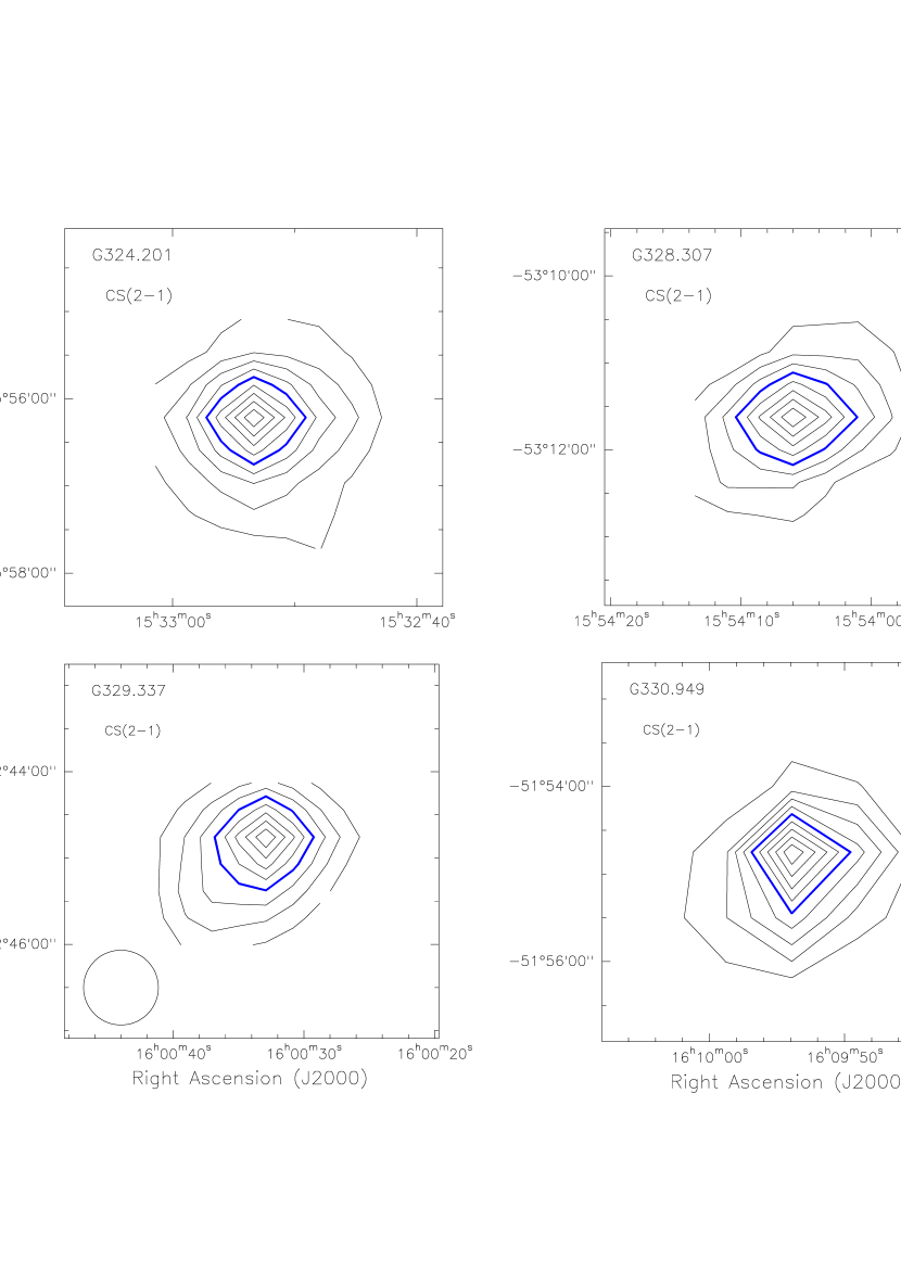
Figure 9: Contour maps of the CS(2$\rightarrow$1) velocity integrated ambient gas emission. Contour levels are drawn in steps of 10% and up to 90% of the peak value. The FWHM beam is shown in the bottom left corner of the lower left panel. Upper left: G324.201+0.119. Peak: 20.8 K  km s${}^{-1}~{}$. Upper right: G328.307+0.423. Peak: 25.6 K  km s${}^{-1}~{}$. Starting contour level: 20%. Lower left: G329.337+0.147. Peak: 28.0 K  km s${}^{-1}~{}$. Starting contour level: 20%. Lower right: G330.949-0.174. Peak: 39.7 K  km s${}^{-1}~{}$.

Fig. 9 shows contour maps of the velocity integrated ambient gas emission in the CS(2$\rightarrow$1) line toward all four regions. The 50% contour level of the emission is marked with dark lines. In all cases the emission, at the resolution of 52″, arises form a single source exhibiting a simple morphology. The deconvolved major and minor FWHM angular sizes determined by fitting a Gaussian profile to the emission are given in §3.3.

3.2 Dust continuum

Fig. 10 presents maps of the 1.2-mm continuum emission, within regions of typically $4^{\prime}$ in size, towards the four observed sources. Emission was detected toward all four regions. The extent and morphology of the 1.2-mm dust continuum emission is similar to that of the CS$(2\rightarrow 1)$ line emission, indicating that these two probes trace the same physical conditions. The observed parameters of the 1.2-mm sources are given in Table 6. Cols.(2) and (3) give their peak position. Cols.(4) and (5) give, respectively, the peak flux density and the total flux density, the later measured directly from the maps using the AIPS tasks IMEAN. Col.(6) gives the deconvolved major and minor FWHM angular sizes determined by fitting a single Gaussian profile to the whole spatial distribution, except for G329.337 for which two Gaussian components were fitted.

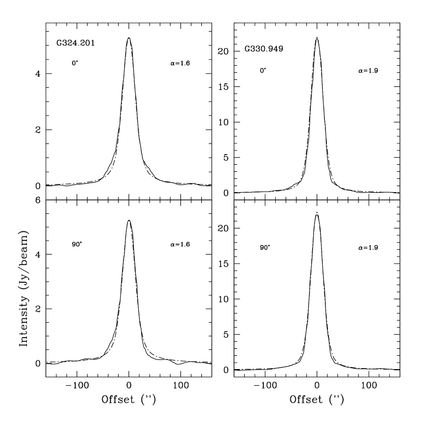
Figure 11: Intensity cuts of the 1.2-mm emission across two orthogonal directions passing through the peak position of G324.201+0.119 (left panels) and G330.949-0.174 (right panels). The position angle of the slices are given in the upper left corner of each panel. Dotted lines correspond to fits of the observed radial intensity with single power-law intensity profiles. The fitted power-law indices are given in the upper right corner of each panel.

In three of the four regions the morphology of the dust emission can be described as arising from a bright compact peak surrounded by an extended envelope of weaker emission, which is characteristic of sources with centrally condensed density profiles. This is illustrated in Fig. 11 which shows slices of the observed 1.2-mm intensity across the two sources with nearly circular morphology (G324.201 and G330.949). We find that the observed radial intensity profiles can be well fitted with single power-law intensity profiles of the form $I\propto r^{-\alpha}$, where $r$ is the distance from the center, properly convolved with the beam of 24″. We derive $\alpha$ indices of 1.6 and 1.9 for the G324.201 and G330.949 cores, respectively. For the G328.307 core an $\alpha$ index of 1.5 has been already derived by Garay et al. (2007).

3.3 Individual sources

Three of the high-mass star forming regions investigated here, G324.201, G329.337 and G330.949, are in the list of $\sim$2000 massive young stellar objects (MYSO) candidates compiled by the RMS survey based on a colour selection criteria of MSX point sources (Hoare et al. 2005). Radio continuum observations have, however, shown that all four Norma cores are associated with compact radio sources, indicating that they are in a more advanced stage of evolution in which an UCHII region has already developed (Walsh et al. 1998; Garay et al. 2006; Urquhart et al. 2007). In all cases the compact radio sources are found projected at the peak position of the 1.2-mm dust continuum emission, suggesting that massive stars are located at the center of the massive and dense cores. In what follows we discuss the characteristics of the molecular gas and dust emission, as well as of the radio emission, toward each of the IRAS sources, individually.

G324.201+0.119.$-$ The G324.201+0.119 massive core is associated with the IRAS source 15290-5546, which has a total luminosity of $5.9\times 10^{5}{\cal L}_{\odot}$. The CS profiles across the core show emission from a nearly Gaussian component, with central velocities of $\sim-88.4$  km s${}^{-1}~{}$and FWHM widths of $\sim 4.0$ km s${}^{-1}~{}$. The spatial distribution of the emission in the CS($2\rightarrow 1$) line from the ambient gas is slightly elongated, with FWHM deconvolved major and minor axis of 43″ and 30″, respectively. The morphology of the 1.2-mm dust emission also shows the presence of a single structure with FWHM deconvolved major and minor axis of 35″ and 28″, respectively. A power-law fit to the 1.2-mm intensity profile gives an index of 1.6 (see Fig. 11). The total flux density of the region at 1.2 mm is 17.3 Jy.

Toward the center of the core the Gaussian component is superposed on a broader and weaker component. In the CS($3\rightarrow 2$) line the wing emission extends up to a flow velocity of $-13.1$  km s${}^{-1}~{}$ in the blue side and 11.4  km s${}^{-1}~{}$ in the red side. The flow velocity, $v_{flow}$, is defined as $v_{flow}=v-v_{o}$, where $v_{o}$ is the ambient cloud velocity. The SiO line profiles are, on the other hand, dominated by the emission from the broad component, covering a flow velocity range from $-12.6$ to $16.8$  km s${}^{-1}~{}$.

Radio continuum observations towards G324.201+0.119 show the presence of two compact radio sources: a cometary-like component, with an angular diameter of $\sim$4”, located at the center of the core and an unresolved component located $\sim$6” north of the former (Urquhart et al. 2007). If excited by single stars, the rate of UV photons needed to produce the cometary and unresolved regions of ionized gas implies the presence of O7 and O8.5 ZAMS stars, respectively.

G328.307+0.423.$-$ The G328.307+0.423 massive core is associated with the IRAS source 15502-5302, which has a total luminosity of $1.1\times 10^{6}{\cal L}_{\odot}$. The spatial distribution of the CS($2\rightarrow 1$) emission from the ambient gas shows an elongated morphology, with FWHM deconvolved major and minor axis of 65″ and 37″, respectively. The elongated morphology is more clearly seen in the observed spatial distribution of the 1.2-mm emission (see Fig. 10), which has FWHM deconvolved major and minor axis of 43″ and 26″, respectively. The total flux density of the region at 1.2-mm is 24.1 Jy.

The CO($1\rightarrow 0$) spectra observed at the center of the core show a double peaked profile, with a strong blueshifted peak at the velocity of $-93.9$  km s${}^{-1}~{}$and a weaker redshifted peak at the velocity of $-88.5$  km s${}^{-1}~{}$. On the other hand, the spectra of the optically thin C¹⁸O($1\rightarrow 0$) line show a single Gaussian profile with a peak velocity of -92.6  km s${}^{-1}~{}$. These spectral characteristics indicate the presence of infall motions (Leung & Brown 1977, Walker, Narayanan, & Boss 1994, Myers et al. 1996). Using expression (9) of Myers et al. (1996) we derive an infall velocity of $\sim 0.3$  km s${}^{-1}~{}$. The profiles of the CS and C³⁴S emission observed across the core are generally asymmetric, showing a peak at velocities of $\sim-92.8$  km s${}^{-1}~{}$and a shoulder toward redshifted velocities. The observed shapes are consistent with the infall motions suggested by the CO($1\rightarrow 0$) emission but for transitions with smaller optical depths. In addition to infalling gas, outflowing gas is clearly detected toward the central region. In the CS(3$\rightarrow$2) line, blueshifted and redshifted emissions are detected up to flow velocities of $-8.2$  km s${}^{-1}~{}$ and 12.2  km s${}^{-1}~{}$, respectively. The SiO emission, which is detected in the velocity range from $-100.0$ to $-82.6$  km s${}^{-1}~{}$, arises mainly from the outflow component, but a narrower component from the ambient core gas is also present.

Radio continuum observations towards G328.307+0.423 show the presence of a complex region of ionized gas, consisting of a handful of low brightness, extended components and a bright, compact component located at the center of the core (Garay et al. 2006). The flux density of the later component increases with frequency whereas its angular size decreases with frequency. These characteristics suggest the presence of a steep gradient in the electron density.

G329.337+0.147.$-$ The G329.337+0.147 massive core is associated with the IRAS source 15567-5236, which has a total luminosity of $1.2\times 10^{6}{\cal L}_{\odot}$. The CS profiles across the core show emission from a bright component with a central velocity of $\sim-107.7$  km s${}^{-1}~{}$and a FWHM width of $\sim 4.5$  km s${}^{-1}~{}$. Strong high velocity wing emission is detected toward the central region in all observed species (see Fig. 7). The blueshifted and redshifted emissions extend up to flow velocities of $-27.6$  km s${}^{-1}~{}$ and $24.2$  km s${}^{-1}~{}$ in the CO(1$\rightarrow$0) line, $-14.8$  km s${}^{-1}~{}$and $16.8$  km s${}^{-1}~{}$ in the CS(3$\rightarrow$2) line, and $-19.2$  km s${}^{-1}~{}$ and 17.4  km s${}^{-1}~{}$ in the SiO(3$\rightarrow$2) line.

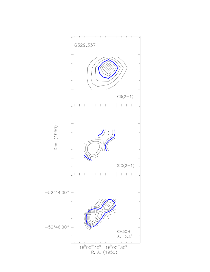
Figure 12: Contour maps of velocity integrated ambient molecular gas emission towards G329.337+0.147. Contour levels are drawn at 20, 30, 40, 50 60, 70, 80 and 90% of the peak value. The star marks the position of the radio source detected by Walsh et al. (1997). Upper: CS(2$\rightarrow$1). Peak value: 28.0 K  km s${}^{-1}~{}$. Center: SiO(2$\rightarrow$1). Peak value: 1.45 K  km s${}^{-1}~{}$. Lower: CH₃OH $3_{0}\rightarrow 2_{0}$ A⁺. Peak value: 3.65 K  km s${}^{-1}~{}$.

The CS($2\rightarrow 1$) emission from the ambient gas arises from a structure that is slightly elongated in the SE direction, with deconvolved FWHM major and minor axis of 44″ and 39″, respectively. The peak of the CS emission is coincident with a methanol maser (Walsh et al. 1997). The spatial distribution of the silicon monoxide and methanol emission show notable differences with respect to that of the emission in carbon monosulfide. The morphology of the SiO and CH₃OH emission shows a double peaked structure, with the main peak being displaced from the peak of the CS emission by $\sim$ 60″ toward the southeast (see Fig. 12). The secondary SiO peak coincides with the peak of the CS emission. The double peaked morphology is also clearly seen in the map of the dust continuum emission.

Radio continuum observations towards G329.337+0.147 show the presence of a single source, with an angular diameter of $6.3\times 4.8$”, exhibiting an irregular multi-peaked morphology (Walsh et al. 1998; Urquhart et al. 2007). If excited by a single star, the rate of UV photons required to ionize this region implies the presence of an O6.5 ZAMS star.

G330.949-0.174.$-$ The G330.949-0.174 massive core is associated with the IRAS source 16060-5146, which has a total luminosity of $1.0\times 10^{6}{\cal L}_{\odot}$. The CS(2$\rightarrow$1) line exhibit an asymmetric profile, with a peak at the velocity of $-92.1$  km s${}^{-1}~{}$and a shoulder toward redshifted velocities. The CS(3$\rightarrow$2) and CS(5$\rightarrow$4) profiles are double peaked, with peaks at $\sim-93.0$  km s${}^{-1}~{}$and $\sim-89.1$  km s${}^{-1}~{}$. The blue peak is stronger than the red peak by a factor of $\sim$ 1.5. The profiles of the C³⁴S and SiO emission are, on the other hand, more symmetric, with peak velocities lying between the two velocity peaks of the CS emission. This result indicates that the complex CS profiles are produced by optical depth effects rather than being due to two velocity components along the line of sight.

The presence of a high velocity gas toward the central region is clearly indicated by the profiles of the CS and SiO emission. In CO lines the outflow emission is blended with emission from less dense molecular clouds in the line of sight. The emission in the CS($3\rightarrow 2$) line extends up to a velocity of $-75.7$  km s${}^{-1}~{}$in the red side and up to a velocity of $-106.0$  km s${}^{-1}~{}$in the blue side.

The spatial distribution of the CS($2\rightarrow 1$) emission from the ambient gas is nearly circular, with FWHM deconvolved major and minor axis of 43″. The circular morphology is also seen in the 1.2-mm dust emission, which exhibits a single structure with FWHM deconvolved major and minor axis of 33″. The total flux density of the region at 1.2 mm is 47.2 Jy. A power-law fit to the 1.2-mm intensity profile gives an index of $1.9\pm 0.1$ (see Fig. 11). The peak of the molecular and dust emissions are displaced about 30″ east of the IRAS position, but are coincident with the position of a methanol maser and a compact radio continuum source (Walsh et al. 1997, 1998). The radio continuum observations of Urquhart et al. (2007) towards G330.949-0.174 show the presence of two compact sources: a bright cometary-like component, with an angular diameter of $\sim$3”, located near the center of the core and an unresolved, weak component, located $\sim$12” northeast of the former. If excited by single stars, the rate of UV photons needed to produce the cometary and unresolved regions of ionized gas implies the presence of O7 and B0 ZAMS stars, respectively.

4 DISCUSSION

4.1 Spectral Energy Distributions

Fig. 13 shows, for each of the 4 sources, the spectral energy distribution (SED) from 12 $\mu$m to 1.2 mm. In this wavelength range the emission is mainly due to thermal dust emission. The flux densities at 12, 25, 60 and 100 µm correspond to IRAS data, and those at 8.3, 12.1, 14.7 and 21.3 µm correspond to Midcourse Space Experiment (MSX) data (Price et al. 2001). The IRAS and MSX fluxes were obtained from the IPAC database.

We fitted the SED with modified blackbody functions of the form $B_{\nu}(T_{d})\left[1-\exp(-\tau_{\nu})\right]\Omega_{s}~{},$ where $\tau_{\nu}$ is the dust optical depth, $B_{\nu}(T_{d})$ is the Planck function at the dust temperature $T_{d}$, and $\Omega_{s}$ is the solid angle subtended by the dust emitting region. The opacity was assumed to vary with frequency as $\nu^{\beta}$, i.e. $\tau_{\nu}=\left(\nu/\nu_{o}\right)^{\beta}$, where $\nu_{o}$ is the frequency at which the optical depth is unity. A single temperature model produced poor fits, underestimating the emission observed at wavelengths smaller than 25$\mu$m, and therefore we used a model with two temperature components. Since the regions are likely to present temperature gradients, this is indeed a coarse simplification. However, this model allows us to determine the average dust temperatures representative of each wavelength range. The parameters derived from the fits, namely dust temperature, opacity power-law index, wavelength at which the opacity is unity, and angular size (assuming a Gaussian flux distribution), for the colder dust component are given in Fig. 13.

4.2 Parameters derived from dust observations

The parameters derived from the 1.2-mm observations are summarized in Table 7. The dust temperatures given in col. (2) correspond to the colder temperature determined from fits to the spectral energy distribution (SED). The radius given in col. (3) were computed from the geometric mean of the deconvolved major and minor angular sizes obtained from single Gaussian fits to the observed spatial structure. The masses of the cores, given in col.(4), were derived using the expression, (e.g., Chini, Krügel, & Wargau 1987)

$$M_{g}={{S_{1.2mm}D^{2}}\over{R_{dg}\kappa_{1.2mm}B_{1.2mm}(T_{d})}}~{}~{},$$ (1)

where $S_{1.2mm}$ is the observed flux density at 1.2mm, $\kappa_{1.2mm}$ is the mass absorption coefficient of dust with a value of 1 cm² g^-1 (Ossenkopf & Henning 1994), $R_{dg}$ is the dust-to-gas mass ratio (assuming 10% He) with a value of $0.01$, and $B(T_{d})$ is the Planck function at the dust temperature $T_{d}$. This expression implicitly assumes that the observed emission at 1.2 mm corresponds to optically thin thermal dust emission and that the source is isothermal. The masses derived in this way range from $5\times 10^{3}$ to $1\times 10^{4}$  $M_{\odot}$. Cols. (5) and (6) give, respectively, the average molecular densities and average column densities derived from the masses and radius assuming that the cores have uniform densities. Clearly, this is a rough simplification, since as discussed in §3.2 the massive and dense cores are likely to have steep density gradients. Finally, the continuum optical depth at 1.2-mm is given in col. (7).

4.3 Parameters derived from line observations

4.3.1 Optical depths and column densities of CS and CO

The optical depth in the CS(3$\rightarrow$2) line, $\tau_{32}^{\small CS}$, can be derived from the ratio of observed main beam brightness temperatures in the CS(3$\rightarrow$2) and C³⁴S(3$\rightarrow$2) lines using the expression,

$${{1-\exp(-\tau_{32}^{\small CS}/r)}\over{1-\exp(-\tau_{32}^{\small CS})}}={{[J_{32}^{\small CS}(T_{ex})-J_{32}^{\small CS}(T_{bg})]}\over{[J_{32}^{\small C^{34}S}(T_{ex})-J_{32}^{\small C^{34}S}(T_{bg})]}}{{T_{mb}(C^{34}S)}\over{T_{mb}(CS)}},~{}$$ (2)

where the subscript 32 refers to the $3\rightarrow 2$ transition, $T_{ex}$ is the excitation temperature of the transition, $T_{bg}$ is the background temperature,

$$J_{\nu}(T)=\frac{h\nu}{k}\frac{1}{\exp(h\nu/kT)-1}~{}~{}~{},$$

and $r$ is the $\tau_{32}^{\small CS}/\tau_{32}^{\small C^{34}S}$ optical depth ratio, given by

$$r=a{{\mid\mu^{CS}\mid^{2}}\over{\mid\mu^{C^{34}S}\mid^{2}}}\left\{{{\exp(-12hB^{\small CS}/kT_{ex})}\over{\exp(-12hB^{\small C^{34}S}/kT_{ex})}}\right\}\left\{{{\exp(h\nu_{32}^{\small CS}/kT_{ex})-1}\over{\exp(h\nu_{32}^{\small C^{34}S}/kT_{ex})-1}}\right\}{{(kT_{ex}/hB^{\small C^{34}S}+1/3)}\over{(kT_{ex}/hB^{\small CS}+1/3)}}~{}~{},$$ (3)

where $a$ is the [C³²S/C³⁴S] isotopic abundance ratio, and $\mu$ and $B$ are the permanent dipole moment and the rotational constant of the molecule, respectively. If the excitation temperature is known, the above expressions allow the optical depth to be determined. We avoid the usual approximation that $\tau_{32}\gg 1$, and solve equation (2) using an interpolation procedure, assuming a [C³²S/C³⁴S] abundance ratio of 22.5 (Blake et al. 1994).

The optical depth in the CO($1\rightarrow 0$) line, $\tau_{10}^{\small CO}$, can be derived from the ratio of observed main beam brightness temperatures in the CO($1\rightarrow 0$) and ¹³CO($1\rightarrow 0$) lines in a similar manner as described above (see Bourke et al. 1997, for the appropriate expressions). We assumed a [CO/¹³CO] abundance ratio of 55, corresponding to the average value across the Galactic disk (Wannier et al. 1982). Further, the observations of the J=$1\rightarrow 0$ line emission in the three isotopic species of carbon monoxide (CO, ¹³CO and C¹⁸O) allow to determine the [¹³CO]/[C¹⁸O] isotopic abundance ratio. Using a [CO]/[¹³CO] abundance ratio of 55, we derive [¹³CO]/[C¹⁸O] abundance ratios in the range 8 to 10.

The peak optical depths at the peak position of the massive cores in the CS(3$\rightarrow$2), C³⁴S(3$\rightarrow$2), CO(1$\rightarrow$0) and ¹³CO(1$\rightarrow$0) lines, are given in cols. 2 to 5 of Table 8. They were computed assuming $T_{ex}$ = 40 K. We find that the emission is optically thick in the CS lines and optically thin in the C³⁴S line for all cores. We note that the dependence of the optical depth with excitation temperature is weak. For instance, assuming $T_{ex}$ = 100 K the derived optical depths are only 0.4% larger.

The total column density $N$ of a linear, rigid rotor, molecule can be derived from the optical depth and excitation temperature of a rotational transition at frequency $\nu$, using the expression (e.g. Garden et al. 1991)

$$N=\frac{3h}{8\pi^{3}\mu^{2}}\frac{k(T_{ex}+hB/3k)}{(J+1)hB}\frac{\exp(E_{J}/kT_{ex})}{1-\exp(-h\nu/kT_{ex})}\int\tau dv~{}~{},$$ (4)

where $J$ is the rotational quantum number of the lower state. This expression assumes that all energy levels are populated according to local thermodynamic equilibrium (LTE) at the temperature $T_{ex}$. In particular the total column density of the CS molecule is given, in terms of the opacity and excitation temperature of the $3\rightarrow 2$ transition, by

$$N({\rm CS})=5.93\times 10^{11}~{}(T_{ex}+0.39)\frac{\exp(7.05/T_{ex})}{1-\exp(-7.05/T_{ex})}\int\tau_{32}^{\small CS}~{}dv~{}~{},$$ (5)

where $v$ is measured in  km s${}^{-1}~{}$. Col. 2 of Table 9 gives the derived CS column density through the center of the cores. The CO column density through the center of the cores are given in col. 3 of Table 9. They were determined in the same way as the CS column densities using the [CO,¹³CO] pair of observations.

From the column density in CS, N(CS), we can estimate the mass of the cores using the expression,

$$M=N(CS)\left[{{H_{2}}\over{CS}}\right]\mu_{m}~{}m_{H}~{}\pi R^{2}~{}~{},$$ (6)

where $[{{H_{2}}\over{CS}}]$ is the H₂ to CS abundance ratio, $\mu_{m}$ is the mean molecular weight, and $R$ is the core radius. The radii, given in column 2 of Table 10, were computed from the geometric mean of the deconvolved CS(2$\rightarrow$1) angular sizes using the distances given in Table 1. The core masses computed from expression (6), using $[{{H_{2}}\over{CS}}]=3\times 10^{7}$ (see §4.3), are given in col. 3 of Table 10. They range from $4.3\times 10^{3}$ to $1.0\times 10^{4}$  $M_{\odot}$. These masses are in good agreement with those derived from the dust continuum observations.

4.3.2 Rotational temperatures and column densities of methanol and silicon monoxide

The rotational temperature, $T_{rot}$, and the total column density, $N_{T}$, of methanol and silicon monoxide can be computed using a rotational diagram analysis (see e.g., Linke, Frerking & Thaddeus 1978; Blake et al. 1987), with the assumptions of optically thin conditions and local thermodynamical equilibrium (LTE), which relates the integrated line intensity, rotational temperature, and column density via

$$\frac{3k\int T_{mb}dv}{8\pi^{3}\mu^{2}\nu S}=\frac{N_{u}}{g_{u}}=\frac{N_{T}}{Q(T_{rot})}\exp\left(-\frac{E_{u}}{kT_{rot}}\right)~{}~{},$$ (7)

where $\mu$, $\nu$, and $S$ are the transition dipole moment, frequency, and line strength of the transition, respectively, $\int T_{mb}dv$ is the velocity integrated main beam brightness, obtained directly from the observations, $E_{u}$ is the upper state energy, and $Q(T_{rot})$ is the rotational partition function.

Fig. 14 shows rotational diagrams for the CH₃OH emission observed at the peak position of the massive cores. The column densities and rotational temperatures, derived from a linear least squares fit to the data, are given in cols. 4 and 6 of Table 9. The rotational temperatures of methanol range from 12.0 K to 22.6 K. These temperatures are significantly smaller than the temperatures derived from the dust observations, of $\sim$ 40K, indicating that the methanol populations are sub-thermally excited (Bachiller et al. 1995; Avery & Chiao 1996).

From rotational diagram analysis of the SiO emission observed at the peak position of the massive cores we derived column densities and rotational temperatures of both the ambient gas, given in cols. 5 and 7 of Table 9, and flowing molecular gas, given in cols. 8 and 9. The rotational temperatures of the flowing gas are typically two times larger than those of the ambient gas. This is illustrated in Fig. 15, which presents a rotational diagram for the SiO emission observed at the peak position of the G330.949 massive core. In this case the gas giving rise to the narrow emission has a rotational temperature of 11.2$\pm 0.6$ K and a column density of $4.1\times 10^{13}$ cm^-2, whereas the outflowing gas producing the broad emission has a rotational temperature of 24.9$\pm 2.4$ K and a column density of $2.6\times 10^{13}$ cm^-2.

4.3.3 Molecular abundances

The chemical composition of a gas cloud is usually characterized by the fractional abundance of molecules relative to molecular hydrogen, the main constituent of the interstellar gas. The abundance of H₂ is however not directly measured. Our observations allow us, however, to directly determine abundances relative to CO. We compute the abundance of species X relative to CO, [X/CO] (where X = CS, SiO, or CH₃OH), as the ratio of the column density of species X and the CO column density in the same velocity range. For SiO and CH₃OH we use the column densities derived from rotational analysis (see §x.x) whereas for CS and CO we use the column densities derived from the observations of their main and isotopic species (see §4.3.1). Table 11 summarizes the abundances of CS, SiO and CH₃OH relative to CO. To convert [X/CO] to fractional abundances relative to H₂ we will assume [CO/H₂]=$10^{-4}$.

Silicon monoxide. We find that the [SiO/CO] abundance ratio in the ambient gas range from $3\times 10^{-7}$ to $1\times 10^{-6}$. Assuming that [CO/H₂] is $10^{-4}$, then the [SiO/H₂] abundance ratio in the ambient gas ranges between $3\times 10^{-11}$ and $1\times 10^{-10}$. Chemical models predict that both high temperature and shocks can produce enhancements in the gas phase SiO abundance. The abundance of SiO in the ambient gas is likely due to the gas-phase high temperature chemistry that takes place in the hot regions surrounding the recently formed massive stars. Models of gas-phase chemistry of hot molecular cores that takes into account grain mantle evaporation by stellar and/or shock radiation (MacKay 1995), predict [SiO/H₂] abundances of $3\times 10^{-11}$ for gas kinetic temperatures of 100 K and densities of $2\times 10^{6}$ cm^-3.

We also find that the [SiO/CO] abundance ratios in the outflowing gas are similar to those derived in the ambient gas. The abundance of SiO in the high velocity gas is likely to be due to gas phase chemistry behind a shock (Iglesias & Silk 1978; Hartquist et al. 1980; Mitchell & Deveau 1983). The enhancement of the SiO abundance in the high velocity material is probably the result of grain destruction by shocks which releases silicon into the gas phase, allowing SiO to form (Seab & Shull 1983; Schilke et al. 1997; Caselli et al. 1997).

Methanol. We find that the [CH₃OH/CO] abundance ratio in the ambient gas is similar for all observed cores, having a mean value of $6\times 10^{-5}$. Assuming an [H₂/CO] of $10^{4}$, it implies that the [CH₃OH/H₂] abundance ratio in the ambient gas is typically $6\times 10^{-9}$. At temperatures smaller than 100 K, chemistry models predict that the production of CH₃OH in the gas phase yield abundances of only 10^-11 relative to H₂ (Lee et al. 1996). The high abundance of methanol in the cores suggests that the radiation from their embedded luminous stars are producing a substantial evaporation of icy grain mantles. Van der Tak et al. (2000a) found a [CH₃OH/H₂] ratio of a few $10^{-8}$ for hot cores and $\sim 10^{-9}$ for the cores with the lower temperatures. The values obtained for the cores investigated here are in between the values found for dark clouds and hot cores, and may correspond to an average of the values appropriate for the cold envelope mass and hot core mass.

Carbon monosulfide. We find that the [CS/CO] abundance ratio in the ambient gas is similar for all observed cores, having a mean value of $4\times 10^{-4}$. Assuming an [H₂/CO] of $10^{4}$, it implies that the [H₂/CS] abundance ratio in the ambient gas is typically $3\times 10^{7}$. This value is typical of molecular cores associated with UC HII regions and hot cores (van der Tak et al. 2000b).

4.3.4 Structure of the cores

In the previous analysis we have implicitly assumed that the density and temperature are uniform within the massive cores. This is obviously a simplification, since the physical conditions are likely to vary with distance from the center of the core. In fact, the intensity profiles of the dust continuum emission indicate that the cores are highly centrally condensed.

Assuming that cores have density and temperature radial distributions following power laws, then for optically thin dust emission the intensity index ${\alpha}$ is related to the density index $p$ ($n\propto r^{-p}$) and the temperature index $q$ ($T\propto r^{-q}$), by the expression $\alpha=p+Qq-1+\epsilon_{f}$ (Adams 1991; Motte & André 2001), where Q is a temperature and frequency correction factor with a value of $\sim 1.2$ at 1.2-mm and 30 K (Beuther et al. 2002) and $\epsilon_{f}$ is a correction factor to take into account the finite size of the cores. The massive and dense cores investigated here are heated by a cluster of luminous sources located at their central position (Chavarría et al. 2009; Paper II). For this type of objects van der Tak et al. (2000b) found that the temperature decreases with distance following a power-law with an index of 0.4. Adopting this value for $q$ and a value of 0.1 for $\epsilon_{f}$, we then infer, using the above expression, that massive and dense cores have density distributions with power-law indices in the range $1.9-2.3$. Several dust continuum studies have already shown the presence of density gradients within massive and dense cores (e.g., van der Tak et al. 2000b, Mueller et al. 2002, Beuther et al. 2002, Williams et al. 2005). In particular, Beuther et al. (2002) observed a large sample of high-mass protostellar candidates and found that the steeper indices are associated with the more luminous and more massive objects. The steep indices derived for the Norma cores are characteristics of the subgroup of strong molecular sources within Beuther’s sample, which have a mean density index of 1.9. The steep profiles are thought to indicate objects in the collapse and accretion phase.

4.4 Segregation within the massive and dense cores

Given the large mass of the massive and dense cores investigated here, of typically $5\times 10^{3}$ M_⊙, their overall collapse process is likely to produce a protostar cluster. The questions of how an individual massive star forms and how the cluster forms are therefore closely related. The derived properties of massive and dense cores are then important boundary conditions to be taken into account for models and simulations.

For dynamical considerations, the relevant mass of the cores is their total mass, including gas and stars. We have already shown that the mass of gas in the cores determined from two independent methods, one based on dust observations and the other on molecular line observations, are in very good agreement. The determination of the total mass of the cores is not straightforward and is usually estimated assuming that the cores are in virial equilibrium. Masses computed under this assumption, using the observed velocity dispersion and size of the CS(2$\rightarrow$1) emission, are given in column 4 of Table 10. The virial masses are similar, within the errors, to the gas masses, implying that the bulk of the core mass is in the form of molecular gas. We note that the virial masses are in average a factor of 1.5 smaller than the dust or molecular masses which might also indicate that the cores do not have enough support and may be contracting.

In paper II we show that the massive cores investigated here are associated with clusters of embedded stars which exhibit clear mass segregation. The high-mass stars are found concentrated near the center of the core while intermediate mass stars are spread over much larger distances from the core center. Garay et al. (2006) have already reported that massive stars are typically located near the center of the massive and dense cores. The question arises as to whether the massive stars are formed in situ or if their spatial location is a result of dynamical effects.

The characteristics of the cores derived here, namely their high densities, steep density profiles and sizes, together with the relatively low fraction of the total mass in the form of stars, suggest that dynamical friction (also called gravitational drag) produced by the gaseous background onto the stars may play an important role in the orbital evolution of stars (Ostriker 1999, Sanchez-Salcedo & Brandenburg 2001, Kim & Kim 2007). The role of gravitational drag on a gaseous background in the evolution and migration of stars within dense gaseous star forming clouds has been investigated using numerical smooth particle hydrodynamics simulations (Escala et al. 2003, 2004). Simulations have been carried out with initial conditions similar to those of the dense cores investigated here, namely steep cloud density profile ($n(r)\propto r^{-1.8}$) and perturber having masses of 1 % of the total gas mass ($\rm M_{star}\sim 20$ $M_{\odot}$). For a typical cloud mass of $4\times 10^{3}$  $M_{\odot}$ and initial distance of the stars to the center of the cloud of 0.4 pc, the migration timescale for high-mass stars is $4.5\times 10^{5}$ yr. This value is smaller than the estimated ages of the young clusters within the cores of $\sim$ 1 Myr (see paper II). Since the migration timescales for dynamical friction are proportional to the inverse of the perturber’s mass (Binney & Tremaine 1987), intermediate mass stars have migration timescales typically a factor $\sim$ 10 longer than those of high mass stars and greater than the estimated age of the clusters. Therefore, gravitational drag is considerably less effective for intermediate mass stars than for high mass stars. This suggest that in the young embedded stellar clusters only the massive stars have been able to efficiently migrate towards the center due to gravitational drag. We conclude that dynamical interactions of cluster members with the gaseous component of massive and dense cores can explain the observed mass segregation, indicating that the gas play an important role in the dynamic of young cluster members and originating the observed mass segregation.

We can not rule out, however, the hypothesis that the cradles of massive stars are formed by direct accretion at the center of centrally condensed massive and dense cores (McKee & Tan 2003). In their turbulent and pressurized dense core accretion model, the collapse of a massive and dense core is likely to produce the birth of a stellar cluster, with most of the mass going into relatively low-mass stars. The high-mass stars are formed preferentially at the center of the core, where the pressure is the highest, and in short time scales of $\sim 10^{5}$ yrs (Osorio et al. 1999; McKee & Tan 2002).

5 SUMMARY

We undertook molecular line observations in several species and transitions and dust continuum observations, both made using SEST, towards four young high-mass star forming regions associated with highly luminous IRAS point sources with colors of UC HII regions and CS(2$\rightarrow$1) emission. These are thought to be massive star forming regions in early stages of evolution. The objectives were to determine the characteristics and physical properties of the dust clouds in which high-mass stars form. Our main results and conclusions are summarized as follows.

We find that the luminous star forming regions in Norma are associated with molecular gas and dust cores with radii of typically 0.5 pc, masses of $\sim 5\times 10^{3}$ M_⊙, molecular hydrogen densities of typically $\sim 2\times 10^{5}$ cm^-3, column densities of $\sim 5\times 10^{23}$ cm^-2, and dust temperatures of $\sim 40$ K. All the derived physical parameters of the Norma cores, except the last, are similar to those of cores harboring UC HII regions (Hunter et al. 2000; Faúndez et al. 2004). For a sample of about 150 IRAS point sources with colours of UC HII regions and average luminosity of $2.3\times 10^{5}$  $L_{\odot}$, Faúndez et al. (2004) derived an average mass of $5\times 10^{3}$ M_⊙, an average size of 0.4 pc, and an average density of $2\times 10^{5}$ cm^-3. The dust temperature of the Norma cores are however larger than of the Faúndez et al. cores, for which they find an average temperature of 32 K. The larger values derived for the Norma cores are consistent with them being centrally heated by more luminous objects (average luminosity of $9.7\times 10^{5}$  $L_{\odot}$).

We find that the observed radial intensity profiles of the dust continuum emission from the Norma cores are well fitted with single power-law profiles, with intensity indices in the range 1.5 to 1.9. This in turn indicates that the cores are highly centrally condensed, having radial density profiles with power-law density indices in the range $1.9-2.3$. These steep profiles are thought to indicate objects in the collapse and accretion phase of evolution.

We find that under the physical conditions of the Norma cores, high-mass stars can migrate towards the central region due to gravitational drag in time scales of $5\times 10^{5}$ yr, smaller than the estimated ages of the clusters, providing an explanation for the observed stellar mass segregation within the cores (Paper II).

Table 1: OBSERVED SOURCES

Source	IRAS	$\alpha$(2000)	$\delta$(2000)	D	$\cal{L}_{\small IRAS}$
				(kpc)	( $L_{\odot}$)
G324.201+0.119	15290-5546	$15^{\rm h}32^{\rm m}53\fs 2$	$-55\arcdeg 56\arcmin 13\arcsec$	6.0	$5.9\times 10^{5}$
G328.307+0.423	15502-5302	15  54  06.3	$-$53 11 38	5.6	$1.1\times 10^{6}$
G329.337+0.147	15567-5236	16  00  33.4	$-$52 44 45	7.0	$1.2\times 10^{6}$
G330.949-0.174	16060-5146	16  09  49.1	$-$51 54 45	5.4	$1.0\times 10^{6}$

Table 2: MOLECULAR LINES: OBSERVATIONAL PARAMETERS

Molecule	Transition	Frequency	Beam Size	$\eta$	$\Delta v$
		(MHz)	(FWHM ″)		( km s${}^{-1}~{}$)
CS	$J=2\rightarrow 1$	97980.968	52	0.73	0.132
	$J=3\rightarrow 2$	146969.049	34	0.66	0.085
	$J=5\rightarrow 4$	244935.606	22	0.45	0.053
C34S	$J=3\rightarrow 2$	144617.147	34	0.66	0.087
SiO	$J=2\rightarrow 1$	86846.998	57	0.75	0.144
	$J=3\rightarrow 2$	130268.702	40	0.68	0.098
CH3OH	$J_{k}=2_{0}\rightarrow 1_{0}$ A+	96741.42	52	0.73	0.129
	$J_{k}=3_{-1}\rightarrow 2_{-1}$ E	145097.470	34	0.66	0.086
CO	$J=1\rightarrow 0$	115271.204	45	0.70	0.111
13CO	$J=1\rightarrow 0$	110201.353	47	0.71	0.116
C18O	$J=1\rightarrow 0$	109782.160	47	0.71	0.116

Table 3: INTEGRATION TIMES AND SENSITIVITIES

Line	G324.201			G328.307			G329.337			G330.949
	tin	$\sigma$		tin	$\sigma$		tin	$\sigma$		tin	$\sigma$
	(m)	(K)		(m)	(K)		(m)	(K)		(m)	(K)
CS$(2\rightarrow 1)$	3	0.12		3	0.14		6	0.064		3	0.094
CS$(3\rightarrow 2)$	4	0.065		4	0.071		4	0.065		4	0.057
CS$(5\rightarrow 4)$	5	0.47		3	0.11		6	0.41		5	0.44
C34S$(3\rightarrow 2)$	4	0.074		4	0.068		4	0.068		4	0.049
SiO$(2\rightarrow 1)$	20	0.018		12	0.028		12	0.027		8	0.026
SiO$(3\rightarrow 2)$	12	0.033		22	0.016		22	0.021		4	0.035
CH3OH$(2_{k}\rightarrow 1_{k})$	8	0.037		–	–		4	0.054		4	0.038
CH3OH$(3_{k}\rightarrow 2_{k})$	8	0.043		8	0.045		8	0.044		4	0.049
CO$(1\rightarrow 0)$	1	0.276		1	0.276		1	0.254		1	0.254
13CO$(1\rightarrow 0)$	3	0.072		3	0.071		3	0.068		3	0.076
C18O$(1\rightarrow 0)$	6	0.057		6	0.055		5	0.060		5	0.063

Table 4: MOLECULAR LINES: OBSERVED PARAMETERS

Line	Peak				Average
	T${}_{A}^{*}$	V	$\Delta$v		T${}_{A}^{*}$	V	$\Delta$v
	(K)	( km s${}^{-1}~{}$)	( km s${}^{-1}~{}$)		(K)	( km s${}^{-1}~{}$)	( km s${}^{-1}~{}$)
G324.201+0.119
CS$(2\rightarrow 1)$	$1.79\pm$0.12	$-88.44\pm$.04	$4.1\pm$0.3		$0.537\pm$.02	$-88.16\pm.03$	$4.6\pm 0.1$
CS$(3\rightarrow 2)$	$2.17\pm$0.07	$-88.52\pm$.01	$4.1\pm$0.1		$1.31\pm$.02	$-88.34\pm.09$	$4.4\pm 0.1$
CS$(5\rightarrow 4)$	$2.98\pm$0.47	$-87.87\pm$.05	$4.4\pm$0.1		$2.33\pm$0.16	$-88.33\pm.04$	$3.8\pm 0.1$
C34S$(3\rightarrow 2)$	$0.745\pm$0.074	$-88.59\pm$.05	$3.6\pm$0.1		$0.276\pm.02$	$-88.33\pm.05$	$3.4\pm 0.2$
SiO$(2\rightarrow 1)$	$0.052\pm$0.018	$-87.4\pm$0.3	$6.1\pm$1.1		$0.025\pm.006$	$-88.74\pm.18$	$3.4\pm 0.5$
SiO$(3\rightarrow 2)$	–	–	–		$0.017\pm.011$	$-88.6\pm 0.3$	$2.6\pm 0.7$
CH3OH$(2_{0}\rightarrow 1_{0})$A+	$0.380\pm$0.037	$-88.26\pm$.05	$4.6\pm$0.2		$0.270\pm.012$	$-88.19\pm.02$	$4.2\pm 0.1$
CH3OH$(3_{0}\rightarrow 2_{0})$A+	$0.510\pm$0.043	$-88.36\pm$.03	$5.5\pm$0.1		$0.277\pm.014$	$-88.24\pm.02$	$4.4\pm 0.1$
G328.307+0.423
CS$(2\rightarrow 1)$	–	–c	–		$0.858\pm 0.028$	$-92.65\pm.03$	$6.3\pm 0.1$
CS$(3\rightarrow 2)$	$2.93\pm 0.07$	$-92.90\pm$.02	$4.8\pm$0.1		$1.84\pm$0.02	$-92.92\pm.01$	$4.3\pm 0.1$
CS$(5\rightarrow 4)$	$1.18\pm$0.11	$-92.82\pm$.04	$3.6\pm$0.2		–	–	–
C34S$(3\rightarrow 2)$	$0.45\pm 0.068$	$-92.49\pm$.09	$4.4\pm$0.2		$0.386\pm$0.02	$-92.32\pm.03$	$5.3\pm 0.1$
SiO$(2\rightarrow 1)$	$0.086\pm$0.028	$-92.24\pm$.13	$6.5\pm$0.4		–	–d	–
SiO$(3\rightarrow 2)$	$0.099\pm 0.016$	$-92.75\pm$.10	$6.1\pm$0.3		–	–	–
CH3OH$(3_{0}\rightarrow 2_{0})$A+	$0.37\pm$0.045	$-91.84\pm$.05	$5.4\pm$0.1		$0.273\pm 0.011$	$-92.71\pm.02$	$4.9\pm 0.1$
G329.337+0.147
CS$(2\rightarrow 1)$	$3.34\pm$0.06	$-107.69\pm$.02	$4.3\pm$0.1		$1.70\pm$0.01	$-107.58\pm.01$	$5.2\pm 0.1$
CS$(3\rightarrow 2)$	$4.92\pm$0.07	$-107.71\pm$.01	$4.7\pm$0.1		$1.81\pm$0.02	$-107.57\pm.01$	$4.5\pm 0.1$
CS$(5\rightarrow 4)$	$2.23\pm$0.41	$-107.73\pm$.08	$4.5\pm$0.3		$1.91\pm$0.14	$-107.76\pm.04$	$4.6\pm 0.2$
C34S$(3\rightarrow 2)$	$1.15\pm$0.07	$-107.72\pm$.03	$3.6\pm$0.1		$0.246\pm$0.02	$-107.66\pm.02$	$3.0\pm 0.1$
SiO$(2\rightarrow 1)$	$0.104\pm$0.027	$-107.67\pm$.10	$4.2\pm$0.2		$0.067\pm$0.007	$-107.58\pm.05$	$4.5\pm 0.2$
SiO$(3\rightarrow 2)$	$0.125\pm 0.021$	$-107.47\pm$.13	$4.2\pm$0.3		–	–	–
CH3OH$(2_{0}\rightarrow 1_{0})$A+	$0.502\pm$0.054	$-107.51\pm$.04	$3.8\pm$0.1		$0.355\pm$0.014	$-107.50\pm.02$	$4.0\pm 0.1$
CH3OH$(3_{0}\rightarrow 2_{0})$A+	$0.671\pm$0.044	$-107.48\pm$.02	$4.8\pm$0.1		$0.322\pm 0.012$	$-107.48\pm.02$	$4.5\pm 0.1$
G330.949-0.174
CS$(2\rightarrow 1)$	–	–c	–		$0.585\pm 0.019$	$-91.16\pm.02$	$7.2\pm 0.1$
CS$(3\rightarrow 2)$	–	–c	–		$1.80\pm 0.016$	$-91.65\pm.02$	$7.2\pm 0.1$
CS$(5\rightarrow 4)$	–	–c	–		$3.05\pm 0.15$	$-92.12\pm.03$	$9.0\pm 0.1$
C34S$(3\rightarrow 2)$	$0.624\pm$0.049	$-91.23\pm$.06	$4.8\pm$0.5		$0.270\pm 0.014$	$-91.01\pm.02$	$4.3\pm 0.2$
SiO$(2\rightarrow 1)$	$0.501\pm$0.026	$-90.24\pm$.03	$6.2\pm$0.2		$0.250\pm 0.08$	$-90.3\pm 0.1$	$6.0\pm 0.1$
SiO$(3\rightarrow 2)$	$0.461\pm 0.035$	$-90.56\pm$.01	$6.1\pm$0.2		–	–	–
CH3OH$(2_{0}\rightarrow 1_{0})$A+	$0.985\pm 0.038$	$-90.35\pm$.03	$6.1\pm$0.1		$0.538\pm 0.011$	$-90.3\pm 0.1$	$5.7\pm 0.1$
CH3OH$(3_{0}\rightarrow 2_{0})$A+	$1.24\pm 0.049$	$-90.95\pm$.02	$7.9\pm$0.1		$0.549\pm 0.014$	$-90.7\pm 0.1$	$6.9\pm 0.1$

Table 5: WING EMISSION: VELOCITY EXTENT

Source	Line	Vmin	Vmax	$\Delta$v
	( km s${}^{-1}~{}$)	( km s${}^{-1}~{}$)	( km s${}^{-1}~{}$)
G324.201+0.119…	CS$(3\rightarrow 2)$	$-$101.5	$-$77.0	24.5
	SiO$(2\rightarrow 1)$	$-$101.0	$-$71.6	29.4
	SiO$(3\rightarrow 2)$	$-$101.4	$-$72.0	29.4
G328.307+0.423…	CS$(3\rightarrow 2)$	$-$101.0	$-$80.6	20.4
	SiO$(2\rightarrow 1)$	$-$100.0	$-$82.6	17.4
G329.337+0.147…	CS$(3\rightarrow 2)$	$-$122.5	$-$90.9	31.6
	SiO$(2\rightarrow 1)$	$-$114.0	$-$92.2	21.8
	SiO$(3\rightarrow 2)$	$-126.9$	$-$90.3	36.6
G330.949-0.174	CS$(3\rightarrow 2)$	$-$106.0	$-$75.7	30.3
	SiO$(2\rightarrow 1)$	$-$107.0	$-$70.4	36.6
	SiO$(3\rightarrow 2)$	$-$103.4	$-$75.2	28.2

Table 6: 1.2-MM CONTINUUM EMISSION: OBSERVED PARAMETERS

SIMBA	Peak position			Flux density		Angular size
source	$\alpha$(2000)	$\delta$(2000)		Peak	Total	(″)
				(Jy/beam)	(Jy)
G324.201+0.119	15 32 52.91	-55 56 10.8		5.28	17.3	$35\times 28$
G328.307+0.423	15 54 06.33	-53 11 43.1		6.35	24.1	$43\times 26$
G329.337+0.147A	16 00 33.10	-52 44 46.6		4.35	11.7	$37\times 27$
G329.337+0.147B	16 00 38.68	-52 45 31.7		1.45	4.58	$53\times 38$
G330.949-0.174	16 09 52.41	-51 54 58.5		21.75	47.2	$34\times 33$

Table 7: DUST EMISSION: DERIVED PARAMETERS

SIMBA	Td	Radius	Mass	n(H2)	N(H2)	$\tau_{1.2mm}$
source	(K)	(pc)	(M⊙)	(cm${}^{-3})$	(cm-2)
G324.201+0.119	37.	0.45	$5.0\times 10^{3}$	$2.2\times 10^{5}$	$4.1\times 10^{23}$	0.016
G328.307+0.423	42.	0.46	$5.2\times 10^{3}$	$2.2\times 10^{5}$	$4.2\times 10^{23}$	0.017
G329.337+0.147A	40.	0.53	$4.1\times 10^{3}$	$1.1\times 10^{5}$	$2.5\times 10^{23}$	0.010
G329.337+0.147B	40.	0.76	$1.6\times 10^{3}$	$1.5\times 10^{4}$	$4.8\times 10^{22}$	0.002
G330.949-0.174	37.	0.44	$1.1\times 10^{4}$	$5.3\times 10^{5}$	$9.6\times 10^{23}$	0.038

Table 8: MOLECULAR LINES: OPACITIES

Source	Peak optical depth
	CS(3$\rightarrow$2)	C34S(3$\rightarrow$2)	CO(1$\rightarrow$0)	13CO(1$\rightarrow$0)
G324.201+0.119	7.0	0.30	42	0.7
G328.307+0.423	3.4	0.15	$>26$	$>0.4$
G329.337+0.147	5.5	0.24	31	0.5
G330.949-0.174	7.1	0.31	69	1.1

Table 9: COLUMN DENSITIES AND ROTATIONAL TEMPERATURES^a

Source	Ambient gas							Outflow
	N(CS)	N(CO)	N(CH3OH)	N(SiO)	T(CH3OH)	T(SiO)		N(SiO)	T(SiO)
G324.201+0.119	$7.6\times 10^{15}$	$1.7\times 10^{19}$	$9.7\times 10^{14}$	—	12.0	—		$1.3\times 10^{13}$	31.0
G328.307+0.423	$5.2\times 10^{15}$	$1.4\times 10^{19}$	$9.4\times 10^{14}$	$4.7\times 10^{12}$	10.3	6.3		$3.8\times 10^{12}$	24.3
G329.337+0.147	$5.8\times 10^{15}$	$1.4\times 10^{19}$	$9.0\times 10^{14}$	$6.3\times 10^{12}$	17.0	16.7		$1.8\times 10^{12}$	45.6
G330.949-0.174	$1.6\times 10^{16}$	$3.9\times 10^{19}$	$2.1\times 10^{15}$	$4.1\times 10^{13}$	22.6	11.2		$2.6\times 10^{13}$	24.9

Table 10: MOLECULAR LINES: DERIVED PARAMETERS OF CORES

Source	Radius	Massa
		MCS	Mvir
	(pc)	( $M_{\odot}$)	( $M_{\odot}$)
G324.201+0.119	0.52	$4.3\times 10^{3}$	$2.3\times 10^{3}$
G328.307+0.423	0.66	$4.6\times 10^{3}$	$5.5\times 10^{3}$
G329.337+0.147	0.71	$6.0\times 10^{3}$	$4.0\times 10^{3}$
G330.949-0.174	0.56	$1.0\times 10^{4}$	$6.1\times 10^{3}$

Table 11: ABUNDANCE RATIOS

Source	CS/CO	SiO/CO	CH3OH/CO
G324.201+0.119	$4.5\times 10^{-4}$	—	$5.7\times 10^{-5}$
G328.307+0.423	$3.7\times 10^{-4}$	$3.3\times 10^{-7}$	$6.7\times 10^{-5}$
G329.337+0.147	$4.1\times 10^{-4}$	$4.5\times 10^{-7}$	$6.4\times 10^{-5}$
G330.949-0.174	$4.1\times 10^{-4}$	$1.0\times 10^{-6}$	$5.4\times 10^{-5}$

Figure 1: Spectral maps of the molecular line emission from G324.201+0.119. The grid spacing is 30″ for all lines, except CS(2$\rightarrow$1) which is 45″. Offsets are from the reference position at $\alpha_{2000}=15^{\rm h}32^{\rm m}53\fs 2,\delta_{2000}=-55\arcdeg 56\arcmin 13\arcsec$. The velocity scale ranges from $-120$ to $-60$  km s${}^{-1}~{}$. The antenna temperature scale ranges from $-0.5$ to 3.5 K for CS(2$\rightarrow$1), $-0.25$ to 3.6 K for CS(3$\rightarrow$2), $-0.2$ to 1.0 K for C³⁴S(3$\rightarrow$2), $-0.03$ to 0.12 K for SiO(2$\rightarrow$1), $-0.06$ to 0.18 K for SiO(3$\rightarrow$2), $-0.1$ to 0.45 K for CH₃OH($2_{k}-1_{k}$), and $-0.1$ to 0.60 K for CH₃OH($3_{k}-2_{k}$).

Figure 2: Spectral maps of the molecular line emission from G328.307+0.423. The grid spacing is 30″ for all lines, except CS(2$\rightarrow$1) which is 45″. Offsets are from the reference position at $\alpha_{2000}=15^{\rm h}54^{\rm m}06\fs 3,\delta_{2000}=-53\arcdeg 11\arcmin 38\arcsec$. The velocity scale ranges from $-120$ to $-65$  km s${}^{-1}~{}$. The antenna temperature scale ranges from $-0.5$ to 4.0 K for CS(2$\rightarrow$1), $-0.5$ to 5.0 K for CS(3$\rightarrow$2), $-0.2$ to 0.9 K for C³⁴S(3$\rightarrow$2), $-0.04$ to 0.13 K for SiO(2$\rightarrow$1), and $-0.1$ to 0.55 K for CH₃OH($3_{k}-2_{k}$).

Figure 3: Spectral maps of the molecular line emission from G329.337+0.147. The grid spacing is 30″ for all lines, except CS(2$\rightarrow$1) which is 45″. Offsets are from the reference position at $\alpha_{2000}=16^{\rm h}00^{\rm m}33\fs 4,\delta_{2000}=-52\arcdeg 44\arcmin 45\arcsec$. The velocity scale ranges from $-135$ to $-70$  km s${}^{-1}~{}$. The antenna temperature scale ranges from $-0.3$ to 4.5 K for CS(2$\rightarrow$1), $-0.6$ to 6.1 K for CS(3$\rightarrow$2), $-0.2$ to 1.4 K for C³⁴S(3$\rightarrow$2), $-0.04$ to 0.21 K for SiO(2$\rightarrow$1), $-0.12$ to 0.90 K for CH₃OH($3_{k}-2_{k}$), and $-0.12$ to 0.65 for CH₃OH($2_{k}-1_{k}$).

Figure 4: Spectral maps of the molecular line emission from G330.949-0.174. The grid spacing is 30″ for all lines, except CS(2$\rightarrow$1) which is 45″. Offsets are from the reference position at $\alpha_{2000}=16^{\rm h}09^{\rm m}49\fs 1,\delta_{2000}=-51\arcdeg 54\arcmin 45\arcsec$. The velocity scale ranges from $-115$ to $-65$  km s${}^{-1}~{}$. The antenna temperature scale ranges from $-0.5$ to 4.8 K for CS(2$\rightarrow$1), $-0.6$ to 6.1 K for CS(3$\rightarrow$2), $-0.2$ to 2.0 K for C³⁴S(3$\rightarrow$2), $-0.07$ to 0.75 K for SiO(2$\rightarrow$1), $-0.15$ to 1.5 K for CH₃OH($3_{k}-2_{k}$), and $-0.15$ to 1.1 for CH₃OH($2_{k}-1_{k}$).

Figure 5: Spectra observed at the peak position of G324.201+0.119. Transitions are given in the upper right corner. The vertical dotted line indicates the systemic velocity of the ambient gas.

Figure 6: Spectra observed at the peak position of G328.307+0.423. Transitions are given in the upper right corner. The vertical dotted line indicates the systemic velocity of the ambient gas.

Figure 7: Spectra observed at the peak position of G329.337+0.147. Transitions are given in the upper right corner. The vertical dotted line indicates the systemic velocity of the ambient gas.

Figure 8: Spectra observed at the peak position of G330.949-0.174. Transitions are given in the upper right corner. The vertical dotted line indicates the systemic velocity of the ambient gas.

Figure 10: SEST/SIMBA maps of the 1.2-mm dust continuum emission. Contour levels are drawn at 5, 10, 20, 30, 40, 50 60, 70, 80 and 90% of the peak flux density. The FWHM beam is shown at the bottom left. In all panels, except the upper right, the stars mark the positions of the compact radio continuum sources detected by Urquhart et al. (2007). Upper left: G324.201+0.119. Peak: 5.28 Jy beam^-1. Upper right: G328.307+0.423. Peak: 6.35 Jy beam^-1. The star marks the position of the bright compact radio continuum source detected by Garay et al. (2006). Lower left: G329.337+0.147. Peak: 4.35 Jy beam^-1. Lower right: G330.949-0.174. Peak: 21.8 Jy beam^-1.

Figure 13: Spectral energy distributions. Stars mark IRAS fluxes, squares MSX fluxes, and the circle the SIMBA flux. The long-dashed curve is a fit to the spectrum using two modified blackbody functions of the form $B_{\nu}(T_{d})\left[1-\exp(-(\nu/\nu_{o})^{\beta})\right]$, with different temperatures. The short-dashed line indicates the fit for the colder temperature component (fit parameters indicated on the upper left).

Figure 14: Rotational diagrams for the methanol emission observed toward the massive cores. The lines correspond to least squares linear fits to the observed data. The derived values of the rotational temperature and total column density are given in Table 11.

Figure 15: Rotational diagram for the narrow (squares) and broad (stars) SiO emission observed towards the G330.949-0.174 massive core. The lines correspond to least squares linear fits to the observed data. The derived values of the rotational temperature are given in the lower left corner.

References

- (1)
- (2)
- (3) Adams, F.C. 1991, ApJ, 382, 544
- (4) Avery, L. W., & Chiao, M. 1996, ApJ, 463, 642
- (5) Bachiller, R., Liechti, S., Walmsley, C. M., & Colomer, F. 1995, A&A, 295, L51
- (6) Beuther, H., Schilke, P., Menten, K. M., Motte, F., Sridharan, T. K., & Wyrowski, F. 2002, ApJ, 566, 945
- (7) Binney J. & Tremaine, S., 1987, Galactic Dynamics, Princeton University Press
- (8) Blake, G.A., van Dishoek, E.F., Jansen, D.J., Groesbeck, T.D., & Mundy, L.G. 1994, ApJ, 428, 680
- (9) Blake, G. A., Sutton, E. C., Masson, C. R., & Phillips, T. G. 1987, ApJ, 315, 621
- (10) Bourke, T. L., Garay, G., Lehtinen, K. K., Köhnenkamp, I., Launhardt, R., Nyman, L-Å, May, J., Robinson, G., & Hyland, A. R. 1997, ApJ, 476, 781
- (11) Bronfman, L., Alvarez, H., Cohen, R. S., & Thaddeus, P. 1989 ApJS, 71, 481
- (12) Bronfman, L., Nyman, L.Å., & May, J. 1996, A&AS, 115, 81
- (13) Caselli, P., Hartquist, T. W., & Havnes, O. 1997, A&A, 322, 296
- (14) Chavarría, L., Mardones, D., Garay, G. et al. 2009 (Paper II)
- (15) Chini, R., Krügel, E., & Wargau, W. 1987, A&A, 181, 378
- (16) Downes, D., Genzel, R., Hjalmarson, Å., Nyman, L.Å., & Rönnäng, B. 1982, ApJ, 252, L29
- (17) Escala, A., Larson, R., Coppi, P., et al., 2003, ASPC, 287, 455
- (18) Escala, A., Larson, R., Coppi, P., et al., 2004, ApJ, 607, 765
- (19) Faúndez, S., Bronfman, L., Garay, G., Chini, R., Nyman, L.-Å, & May, J. 2004, A&A, 426, 97
- (20) Garay, G., Brooks, K.J., Mardones, D. & Norris, R.P. 2006, ApJ, 651, 914
- (21) Garay, G., Mardones, D., Brooks, K.J., Videla, L., & Contreras, Y. 2007, ApJ, 666, 309
- (22) Garden, R.P., Hayashi, M., Gatley, I., & Hasegawa, T. 1991, ApJ, 374, 540
- (23) Harju, J., Lehtinen, K., Booth, R.S., & Zinchenko, I. 1998, A&AS, 132, 211
- (24) Hartquist, T.W., Oppenheimer, M., & Dalgarno, A. 1980, ApJ, 236, 182
- (25) Hoare, M.G., Lumsden, S.L., Oudmaijer, R.D., Urquhart, J.S. et al. 2005, in Massive star birth: A crossroads of Astrophysics, Proceedings IAU Symposium No. 227, eds. Cesaroni, R., Felli, M., Churchwell, E., Walmsley, M. (Cambridge: Cambridge University Press), 370
- (26) Hunter, T.R., Churchwell, E., Watson, C., Cox, P., Benford, D.J., & Roelfsema, P.R. 2000, AJ, 119, 2711
- (27) Iglesias, E., & Silk, J. 1978, ApJ, 226, 851
- (28) Juvela, M. 1996, A&AS, 118, 191
- (29) Kim, H. & Kim, W-T., 2007, ApJ, 665, 432
- (30) Lee H.-H., Bettens R., Herbst E., 1996, A&AS119, 111
- (31) Leung, C.M., & Brown, R.L. 1977, ApJ, 214, L73
- (32) Liechti, S. & Walmsley, C.M. 1997, A&A, 321, 625
- (33) Linke, R. A., Frerking, M. A., & Thaddeus, P. 1978, ApJ, 234, L139
- (34) MacKay, D.D.S. 1995, MNRAS, 274, 694
- (35) McKee, C.F., & Tan, J.C. 2002, Nature 416, 59
- (36) McKee, C.F., & Tan, J.C. 2003, ApJ, 585, 850
- (37) Menten, K.M., Walmsley, C.M., Wilson, T.L., & Henkel, C. 1988, LNP, 315, 261
- (38) Menten, K.M., Pillai, T., & Wyrowski, F. 2005, in Massive star birth: A crossroads of Astrophysics, Proceedings IAU Symposium No. 227, eds. Cesaroni, R., Felli, M., Churchwell, E., Walmsley, M. (Cambridge: Cambridge University Press), 23
- (39) Mitchell, G.F., & Deveau, T.J. 1983, ApJ, 266, 646
- (40) Motte, F., & André, P. 2001, A&A, 365, 440
- (41) Mueller, K.E., Shirley, Y.L., Evans II, N.J. & Jacobson, H.R. 2002, ApJS, 143, 469
- (42) Myers, P.C., Mardones, D., Tafalla, M., Williams, J.P., & Wilner, D.J. 1996, ApJ, 465, L133
- (43) Osorio, M., Lizano, S., & D’Alessio, P. 1999, ApJ, 525, 808
- (44) Ossenkopf, V., & Henning, Th. 1994, A&A, 291, 943
- (45) Ostriker, S., 1999, ApJ, 513, 252
- (46) Plume, R., Jaffe, D.T., & Evans II, N.J. 1992, ApJS, 78, 505
- (47) Plume, R., Jaffe, D.T., Evans II, N.J., Martín-Pintado, J. & Gómez-González, J. 1997, ApJ, 476, 730
- (48) Price, S.D., Egan, M.P., Carey, S.J., Mizuno, D.R., & Kuchar, T.A. 2001, AJ, 121, 2819
- (49) Rathborne, J. M., Jackson, J.M., & Simon, R. 2006, ApJ, 641, 389
- (50) Sánchez-Salcedo, F. & Brandenburg, A., 2001, MNRAS, 322, 67
- (51) Schilke, P., Walmsley, C.M., Pineau des Forêts, G., & Flower, D.R. 1997, A&A, 321, 293
- (52) Shirley, Y.L., Evans II, N.J., Young, K.E., Knez, C., & Jaffe, D.T. 2003, ApJS, 149, 375
- (53) Seab, C.G., & Shull, J.M. 1983, ApJ, 275, 652
- (54) Urquhart, J.S., Busfield, A.L., Hoare, M.G., Lumsden, S.L., Clarke, A.J., Moore, T.J.T., Mottram, J.C. & Oudmaijer, R.D. 2007, A&A461, 11
- (55) van der Tak, F.F.S., van Dishoeck, E.F. & Caselli, P. 2000a, A&A, 361, 327
- (56) van der Tak, F.F.S., van Dishoeck, E.F., Evans II, N.J., & Blake, G.A. 2000b, ApJ, 537, 283
- (57) Walker, C.K., Narayanan, G., & Boss, A.P. 1994, ApJ, 431, 767
- (58) Walsh, A.J., Burton, M.G., Hyland, A.R., & Robinson, G. 1998, MNRAS, 301, 640
- (59) Walsh, A.J., Hyland, A.R., Robinson, G., & Burton, M.G. 1997, MNRAS, 291, 261
- (60) Wannier, P.G., Penzias, A.A., & Jenkins, E.B. 1982, ApJ, 254, 100
- (61) Williams, S.J., Fuller, G.A., & Sridharan, T.K. 2004, A&A, 417, 115
- (62) Williams, S.J., Fuller, G.A., & Sridharan, T.K. 2005, A&A, 434, 257
- (63) Zinchenko, I., Mattila, K. & Toriseva, M. 1995, A&AS, 111, 95
- (64) Ziurys, L.M., Friberg, P., & Irvine, W.M. 1989, ApJ, 343, 201
- (65)