Renormalization and Universality of Van der Waals forces

Abstract

Renormalization ideas can profitably be exploited in conjunction with the superposition principle of boundary conditions in the description of model independent and universal scaling features of the singular and long range Van der Waals force between neutral atoms. The dominance of the leading power law is highlighted both in the scattering as well as in the bound state problem. The role of off-shell two-body unitarity and causality within the Effective Field Theory framework on the light of universality and scaling at low energies is analyzed.

1 Introduction

Van der Waals (VdW) forces were first conjectured from the experimental observation that in an adiabatic expansion a gas of neutral particles cools down (Joule-Thomson effect). Since the inter-particle distance at room temperature is $\sim 30\AA$ this suggests that VdW forces are long range and attractive.  Their genuine quantum mechanical origin and form $\sim 1/r^{6}$ was uncovered by London 1930ZPhy…63..245L as long range dipole fluctuations between charge-neutral atomic and molecular systems. They dominate at distances above $5-10\AA$ and hold atomic dimers together. The relativistic Casimir-Polder forces $\sim 1/r^{7}$ include retardation, are a consequence of vacuum fluctuations Casmir:1947hx and operate at very long distances $\sim 1000-2000\AA$, a relevant scale in colloids. The general field theoretical treatment due to two photon exchange Feinberg:1970zz yielded the so far missing magnetic contribution (For a review see e.g. Feinberg:1989ps ).

Van der Waals forces, besides being long range, diverge if directly extrapolated to short distance scales but a sensible interpretation becomes possible Case:1950an ; Frank:1971xx . Because of the interest on ultra-cold atoms in recent years 2004cucq.book…..W fundamental work for neutral atoms was initiated in Refs. PhysRevA.48.546 ; Gao:1998zza ; PhysRevA.59.1998 (see also 2009PhRvA..80a2702G ) from the point of view of quantum defect theory, where a spectacular reduction of parameters takes place. This is supported by more conventional potential calculations and a pattern of (VdW) universality and scaling sets in Cordon:2009vdw with no explicit reference to short distance scales or cut-offs. Actually, Effective Field Theories (EFT) explicitly exploit the characteristic low energy parameter reduction from the start and yield very general universality patterns which do not resolve the nature of the forces and therefore enjoy a wide applicability Braaten:2004rn ; Braaten:2007nq ; Platter:2009gz . They are based on pure contact (zero range) interactions and discard the long distance tail of VdW forces. In the present contribution we analyze the quantum mechanical problem from the point of view of renormalization, and address to what extent do these contact interactions faithfully describe the underlying Van der Waals force.

2 From Binding to Van der Waals forces

To provide a proper perspective it is interesting to recall the distance scales where we expect the dispersion forces to dominate. For simplicity let us consider the simplest $H_{2}$ molecule, which Hamiltonian in the CM frame and in the Born-Oppenheimer approximation, valid for heavy protons, $m_{p}\gg m_{e}$, reads 

$$H=H_{1}+H_{2}+V_{12}$$ (1)

where the single atom hydrogen-like Hamiltonians are

$$H_{1,2}=-\frac{1}{2m_{e}}\vec{\nabla}_{1,2}^{2}-\frac{\alpha}{|\vec{r}_{1,2}\pm\vec{r}/2|}$$ (2)

with $\vec{r}_{1}$ and $\vec{r}_{2}$ the electron coordinates and

$$V_{12}=\alpha\left[\frac{1}{r}+\frac{1}{|\vec{r}_{1}-\vec{r}_{2}|}-\frac{1}{|\vec{r}_{1}-\vec{r}/2|}-\frac{1}{|\vec{r}_{2}+\vec{r}/2|}\right]$$ (3)

Defining $\vec{r}_{1,\pm}=\vec{r}_{1}\pm\vec{r}/2$ and $\vec{r}_{2,\pm}=\vec{r}_{2}\pm\vec{r}/2$, the solutions to Eq. (2) are $\psi_{n}(\vec{r}_{1,-})$ and $\psi_{m}(\vec{r}_{2,+})$ where $E_{n}=-m_{e}\alpha^{2}/2n^{2}=-13.6{\rm eV}/n^{2}$ 1974-Levine so that for $V_{12}=0$ the total mirror symmetric molecular normalized wave function reads

$$\Psi^{(0)}_{n,m}(\vec{r}_{1},\vec{r}_{2})=\frac{\psi_{n}(\vec{r}_{1,-})\psi_{m}(\vec{r}_{2,+})\pm\psi_{m}(\vec{r}_{1,+})\psi_{n}(\vec{r}_{2,-})}{\sqrt{2(1\pm S_{nm})}}\,,$$

(4)

with $S_{nm}(r)$ the corresponding overlap integral, fulfilling $S_{n,m}(0)=\delta_{n,m}$ and $S_{n,m}={\cal O}(e^{-2r/a_{0}})$. This generates a coupled channel matrix Hamiltonian what eigenvalues provide the H-H adiabatic energy, $E_{\rm HH}(r)\to 2E_{\rm H}$ for $r\to\infty$. The nowadays standard variational approach pioneered by Heitler and London 1927ZPhy…44..455H and culminating with the benchmark determination of the ground state dissociation energy 1960RvMP…32..219K does not accurately work at very long distances, and thus perturbation theory might be preferable. Taking $H_{0}=H_{1}+H_{2}$ as the unperturbed Hamiltonian and $V_{12}$ as the perturbation, one can determine the potential energy shift of the system at a fixed proton-proton separation $r$ in perturbation theory, which to second order reads,

$$V_{\rm H-H}(r)\equiv E_{\rm H-H}(r)-2E_{\rm H}=\Delta E_{1}(r)+\Delta E_{2}(r)+\dots$$ (5)

In the case of the $H_{2}$ molecule the calculation was undertaken in 1930 by London and Eisenschitz 1930ZPhy…60..491E in the closure approximation (CA) . We have reproduced the analytical calculation Alvaro-Tesina and the results are presented in Fig. 1. Already in $\Delta E_{1}(r)$ the finite atomic size yields effects which are $\sim e^{-2r/a_{0}}$.

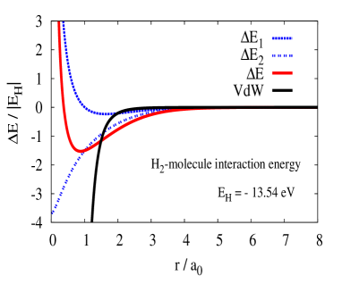
Figure 1: Born-Oppenheimer interaction energies for the $H_{2}$ molecule (in units of the ionization energy of the H atom, $E_{H}=-m_{e}c^{2}\alpha^{2}/2=13.54{\rm eV}$) as a function of distance (in units of the Bohr radius $a_{0}=\hbar^{2}/m_{e}c^{2}=0.51\AA$). We compare first order, $\Delta E_{1}$, and second order, $\Delta E_{2}$, perturbation theory with the pure VdW approximation $\Delta E_{\rm VdW}=-6m_{e}c^{2}\alpha^{2}(a_{0}/r)^{6}$. All calculations use the closure approximation.

An interesting feature is that due to the finite atomic size, $\sim a_{0}$, second order in perturbation theory is finite at zero separation, $|\Delta E_{2}(0)|<\infty$. Actually, for $r\to 0$ we expect the exact behaviour $V_{\rm H-H}(r)-\alpha/r\to E_{\rm He}-2E_{\rm H}$. In the CA we get $E_{\rm He}^{\rm CA}=-110{\rm eV}$ to be compared with $E_{\rm He}^{\rm exact}=-79{\rm eV}$. At large distances only the second order direct term in Eq. (5) contributes yielding,

$$V(r)=-\sum_{n=6}^{\infty}\frac{C_{n}}{r^{n}}+{\cal O}(e^{-2r/a_{0}})$$ (6)

where in the CA $C_{n}=-c_{n}m_{e}c^{2}\alpha^{2}a_{0}^{n}$ with $c_{6}=6$, $c_{8}=135$, $c_{10}=7875/2$, about $5\%$ accurate compared to exact values (see table 1). For $n\gg 6$ one has $C_{n}\sim(a_{0})^{n}n!$ which means that the VdW series represents a diverging asymptotic expansion. As it usually happens in such a case, for a fixed order of the truncation, this poses a lower limit on the distance below which it makes no sense improve the calculation. Usually, only the terms with $n=6,8,10$ are retained.  Calculations show that, so far, corrections are always negative, i.e. $C_{n}>0$ as could be inferred from the Lieb-Thirring universal bound 1986PhRvA..34…40L which establishes that generally $V(r)<-c/r^{6}$ for any pair of atoms with underlying Coulomb forces such as in Eq. (2). The positivity of the $C_{n}$’s will prove essential in what follows. As we see in Fig. 1 in the $H_{2}$ case the Van der Waals force dominates for distances of about $5\AA$. Actually this corresponds to an energy which is comparable to the environmental translational thermal energy $k_{B}T\sim 1/40\,{\rm eV}$ 2003q.bio….12005C . Clearly in the ultra-cold region the VdW force dominates. Therefore, a VdW theory should work in a very broad range of distances and wavelengths.

The VdW potentials are valid assuming large distances $r\gg a_{0}$ and low energies $p^{2}/(2\mu)\ll\Delta=E_{1}-E_{0}$ so that intermediate excited states do not contribute dynamically. Thinking of the molecular wave function like e.g. Eq (4), at large distances we may neglect the exchange term with accuracy ${\cal O}(e^{-r/a_{0}})$, and the coupled channel Hamiltonian reads

$$H_{n^{\prime},m^{\prime};n,m}(r)=(E_{n}+E_{m})\delta_{n^{\prime},n}\delta_{m^{\prime},m}+V_{n^{\prime},m^{\prime};n,m}(r)$$ (7)

This problem may quite generally be decomposed within the total multichannel Hilbert space into the $P$-space (elastic) and $Q$-space (excited) states Lane:1948zh , where $P=|0,0\rangle\langle 0,0|$ and $Q=1-P$ are the corresponding projection operators. This yields the box-matrix structure

$$H_{PP}\Psi_{P}+V_{PQ}\Psi_{Q} = E\Psi_{P}$$

$$V_{QP}\Psi_{P}+H_{QQ}\Psi_{Q} = E\Psi_{Q}$$ (8)

where in the Born-Oppenheimer approximation all these potentials are local functions of the inter-nuclear separation $r$. Eliminating the unobserved channels we get the effective optical potential

$$\bar{V}_{PP}(E)=V_{PP}+V_{PQ}(E-H_{QQ})^{-1}V_{QP}$$ (9)

which develops an imaginary part if the first inelastic threshold becomes open. The important point is that if the complete underlying electronic Hamiltonian, Eq. (1) is energy independent, then for $E=p^{2}/(2\mu)+2E_{\rm H}<E_{\rm H^{*}}+E_{\rm H}$

$$\bar{V}_{PP}^{\prime}(E) = -V_{PQ}(E-H_{QQ})^{-2}V_{QP}<0$$ (10)

The underlying local and energy independent dynamics has consequences in the low energy EFT representations of the VdW interactions (see Section 6).

3 Universal Scaling Theorems

We review here some results found in a previous work PavonValderrama:2005wv ; PavonValderrama:2007nu (for a short review see e.g. RuizArriola:2007wm ),within a nuclear physics and multichannel context which will prove useful in the analysis of VdW forces . Our starting point is the finite energy scattering state Schrödinger’s equation for the relative wave function between two particles of masses $m_{1}$ and $m_{2}$ which interact through a central potential,

$$-u^{\prime\prime}+U(r)u+\frac{l(l+1)}{r^{2}}u=k^{2}u\,,$$ (11)

where $U(r)=2\mu V(r)$, $\mu=m_{1}m_{2}/(m_{1}+m_{2})$ is the reduced mass, $k=p/\hbar=2\pi/\lambda$ the wavenumber and $u(r)$ the reduced wave function. We will neglect finite size and exchange effects and take $V(r)$ given just by Eq. (6) where $C_{n}$ are the standard VdW coefficients which are computed ab initio from electronic orbital atomic structure calculations KMS-data . The potential in Eq. (6) can conveniently be rewritten as

$$U(r)=-\frac{R_{6}^{4}}{r^{6}}\left[1+g_{1}\frac{R_{6}^{2}}{r^{2}}+g_{2}\frac{R_{6}^{4}}{r^{4}}+\dots\right]\,,$$ (12)

where $R_{6}=(2\mu C_{6})^{\frac{1}{4}}$ is the VdW length scale and $g_{1}$, $g_{2}$, etc. represent the contributions from $C_{8}$, $C_{10}$ etc. at $r=R_{6}$ respectively. In table 1 we compile numbers for a bunch of interesting cases. Typically, $R_{6}\sim 10-200\AA$ but also $g_{1}\sim 10^{-2}$ and $g_{2}\sim 10^{-4}$. This raises immediately the question under what conditions the expansion (12) can be truncated in a meaningful way, i.e. when the neglected terms can indeed be considered negligible in scattering and bound state properties. This question is intriguing since at short distances the more singular terms are manifestly more divergent. Actually, the range where $C_{8}$ yields an important correction but $C_{10}$ is still small is $g_{2}^{-1/4}\ll r/R_{6}\ll g_{1}^{-1/2}$ which in view of table 1, $g_{2}\sim g_{1}^{2}$, becomes extremely narrow or inexistent.

Table 1: Reduced di-atomic masses, Van der Waals dispersion coefficients $C_{6}$, $C_{8}$ and $C_{10}$ as well as the leading Van der Waals length scale $R_{6}=(2\mu C_{6})^{\frac{1}{4}}$, and the dimensionless coefficients $g_{1}$ and $g_{2}$ defined by the dimensionless reduced potential $2\mu V(r)R_{6}^{2}\equiv R_{6}^{2}U(r)=-x^{-6}\left[1+g_{1}x^{-2}+g_{2}x^{-4}+\dots\right]$ with $x=r/R_{6}$ the distance in Van der Waals units, of the di-atomic systems used in the present paper. Atomic units are used throughout. The atomic masses have been taken from the National Institute of Standards and Technology http://physics.nist.gov/PhysRefData/Compositions/

Atoms	$\mu(a.u.)$	$C_{6}(a.u.)$	$C_{8}(10^{5}a.u.)$	$C_{10}(10^{7}a.u.)$	$R_{6}(a.u.)$	$g_{1}(10^{-2})$	$g_{2}(10^{-4})$
H-H	918.576	6.499 1996PhRvA..54.2824Y	0.001244 1996PhRvA..54.2824Y	0.0003286 1996PhRvA..54.2824Y	10.4532	17.51760	423.45441
He-He	3648.150	1.461 1996PhRvA..54.2824Y	0.000141 1996PhRvA..54.2824Y	0.00001837 1996PhRvA..54.2824Y	10.1610	9.35937	117.94642
Li-Li	6394.697	1389. 2001PhRvA..63e2704D	0.834 2003JChPh.119..844P	0.735 2003JChPh.119..844P	64.9214	1.42458	2.97874
Na-Na	20953.894	1556. 2001PhRvA..63e2704D	1.160 2003JChPh.119..844P	1.130 2003JChPh.119..844P	89.8620	0.92320	1.11369
K-K	35513.247	3897. 2001PhRvA..63e2704D	4.200 2003JChPh.119..844P	5.370 2003JChPh.119..844P	128.9846	0.64780	0.49784
Rb-Rb	77392.363	4691. 2001PhRvA..63e2704D	5.770 2003JChPh.119..844P	7.960 2003JChPh.119..844P	164.1528	0.45647	0.23370
Cs-Cs	121135.907	6851. 2001PhRvA..63e2704D	10.200 2003JChPh.119..844P	15.900 2003JChPh.119..844P	201.8432	0.36544	0.13983
Fr-Fr	203270.053	5256. 2001PhRvA..63e2704D	6.648 1998PhRvA..58.4259M	10.699 1998PhRvA..58.4259M	215.0006	0.27362	0.09526
Li-Na	9798.954	1467. 2001PhRvA..63e2704D	0.988 2003JChPh.119..844P	0.916 2003JChPh.119..844P	73.2251	1.25605	2.17183
Li-K	10837.871	2322. 2001PhRvA..63e2704D	1.950 2003JChPh.119..844P	2.100 2003JChPh.119..844P	84.2285	1.18374	1.79689
Li-Rb	11813.296	2545. 2001PhRvA..63e2704D	2.340 2003JChPh.119..844P	2.610 2003JChPh.119..844P	88.0587	1.18572	1.70555
Li-Cs	12148.102	3065. 2001PhRvA..63e2704D	3.210 2003JChPh.119..844P	3.840 2003JChPh.119..844P	92.8950	1.21364	1.68241
Na-K	26356.596	2447. 2001PhRvA..63e2704D	2.240 2003JChPh.119..844P	2.530 2003JChPh.119..844P	106.5708	0.80600	0.80155
Na-Rb	32978.812	2683. 2001PhRvA..63e2704D	2.660 2003JChPh.119..844P	3.130 2003JChPh.119..844P	115.3377	0.74528	0.65923
Na-Cs	35727.672	3227. 2001PhRvA..63e2704D	3.620 2003JChPh.119..844P	4.550 2003JChPh.119..844P	123.2277	0.73874	0.61148
K-Rb	48685.873	4274. 2001PhRvA..63e2704D	4.930 2003JChPh.119..844P	6.600 2003JChPh.119..844P	142.8292	0.56543	0.37106
K-Cs	54924.387	5159. 2001PhRvA..63e2704D	6.620 2003JChPh.119..844P	9.400 2003JChPh.119..844P	154.2909	0.53903	0.32152
Rb-Cs	94444.928	5663. 2001PhRvA..63e2704D	7.690 2003JChPh.119..844P	11.300 2003JChPh.119..844P	180.8480	0.41520	0.18654
Cr-Cr	47340.881	733. 2005PhRvL..94r3201W	0.750 2005PhRvL..94r3201W	$-$	91.2731	1.22821	$-$

To determine the solution of Eq. (11) it is necessary to give sensible boundary conditions at the origin and infinity. For the usual regular potentials there are a regular and irregular solution at the origin, and the regularity condition $u(0)=0$ fixes uniquely the solution. However, since the potential is singular and attractive there are two linearly independent solutions, so regularity at the origin does not select a unique solution. Indeed, at short distances the De Broglie wavelength is slowly varying, $d[U(r)]^{-\frac{1}{2}}/dr\ll 1$ and hence a WKB approximation holds Case:1950an ; Frank:1971xx , yielding for $r\to 0$

$$u_{k}(r) \to C\left(\frac{r}{R_{n}}\right)^{n/4}\sin\left[\frac{2}{n-2}\left(\frac{R_{n}}{r}\right)^{\frac{n}{2}-1}+\varphi_{k}\right]\,,$$ (13)

where $R_{n}=(2\mu C_{n})^{1/(n-2)}$ corresponds to the highest VdW scale considered in Eq. (6) (see also Eq. (12). The phase $\varphi_{k}$ is arbitrary and could, in principle, be energy dependent (see below.

To fix ideas we will restrict to $l=0$, $s-$waves. For a positive energy scattering state it is convenient to use the normalization at very long distances given by

$$u_{k}(r)\to\frac{\sin(kr+\delta_{0})}{\sin\delta_{0}}=\cos(kr)+k\cot\delta_{0}\frac{\sin(kr)}{k}\,,$$ (14)

where $\delta_{0}(k)$ is the scattering phase shift for the $l=0$ angular momentum state. For the potential which at long distances behave as Eq. (12) one has the effective range expansion (ERE) 1963JMP…..4…54L

$$k\cot\delta_{0}(k)=-\frac{1}{\alpha_{0}}+\frac{1}{2}r_{0}k^{2}+v_{2}k^{4}\log(k^{2})+\dots$$ (15)

where $\alpha_{0}$ is the scattering length, and $r_{0}$ is the effective range. $\alpha_{0}$ and $r_{0}$ can be calculated from the asymptotic behaviour of the zero energy solution

$$u_{0}(r)\to 1-r/\alpha_{0}\,,$$ (16)

and using the definition

$$r_{0} = 2\int_{0}^{\infty}dr\left[\left(1-r/\alpha_{0}\right)^{2}-u_{0}(r)^{2}\right]\,.$$ (17)

Next, we use the superposition principle of boundary conditions and write

$$u_{k}(r)=u_{k,c}(r)+k\cot\delta_{0}\,u_{k,s}(r)\,,$$ (18)

with $u_{k,c}(r)\to\cos(kr)$ and $u_{k,s}(r)\to\sin(kr)/k$ for $r\to\infty$. At zero energy we have

$$u_{0}(r)=u_{o,c}(r)-u_{0,s}(r)/\alpha_{0}\,,$$ (19)

with $u_{0,c}(r)\to 1$ and $u_{0,s}(r)\to\sin r$ for $r\to\infty$. The short distance phase $\varphi_{0}$ can be fixed in practice introducing a short distance cut-off, $r_{c}$. The way to proceed is as follows. Given a scattering length $\alpha_{0}$ as input one integrates in from large down to small distances, say $r=r_{c}\ll R_{6}$ whence determining $\varphi_{0}$. To determine $\varphi_{k}$ we do the same but for finite energy states. A relation between both short distance phases can be found as follows PavonValderrama:2005wv . If we build $(u_{k}^{\prime}u_{0}-u_{0}^{\prime}u_{0})^{\prime}$ and integrate from $r_{c}$ to infinity and use Eq. (18) and Eq. (19) respectively, one gets

$$\frac{1}{R_{n}}\sin(\varphi_{k}-\varphi_{0}) = k^{2}\int_{0}^{\infty}dr\left[u_{0,c}(r)-\frac{1}{\alpha_{0}}\,u_{0,s}(r)\right]$$ (20)

$$\times\Big{[}u_{k,c}(r)+k\cot\delta_{0}(k)\,u_{k,s}(r)\Big{]}\,,$$

which becomes an orthogonality relation if and only if $\varphi_{k}=\varphi_{0}$. This implies that the corresponding Hamiltonian, although unbounded from below becomes self-adjoint on the domain of square integrable functions which have the short distance behaviour, Eq. (13), with the same short distance phase (a common domain of definition). In other words, the short distance common phase, $\varphi$, labels the particular self-adjoint extension of the Hamiltonian depending on the Van der Waals dispersion coefficients. . One important property is that $\varphi$ is not only energy independent but it must be fixed independently on the long distance potential, and thus encodes all short distance information not accounted for by the truncated potential Eq. (12). Moreover, there is a further remarkable consequence of the energy independence of $\varphi$ obtained by expanding the integrand in Eq. (20),

$$k\cot\delta_{0}(k)=\frac{\alpha_{0}{\cal A}(k)+{\cal B}(k)}{\alpha_{0}{\cal C}(k)+{\cal D}(k)}\,,$$ (21)

whereas the functions ${\cal A}$, ${\cal B}$, ${\cal C}$ and ${\cal D}$ are even functions of $k$ which depend only on the potential and are given by

$${\cal A}(k) = \int_{0}^{\infty}dr\,u_{0,c}(r)u_{k,c}(r)\,,$$ (22)

$${\cal B}(k) = \int_{0}^{\infty}dr\,u_{0,s}(r)u_{k,c}(r)\,,$$ (23)

$${\cal C}(k) = \int_{0}^{\infty}dr\,u_{0,c}(r)u_{k,c}(r)\,,$$ (24)

$${\cal D}(k) = \int_{0}^{\infty}dr\,u_{0,s}(r)u_{k,s}(r)\,.$$ (25)

Note that the dependence of the phase-shift on the scattering length is wholly explicit; $\cot\delta_{0}$ is a bilinear rational mapping of $\alpha_{0}$. This is just a manifestation of the underlying Moebius transformation well known from the theory of ordinary differential equations discussed in PavonValderrama:2007nu . The obvious conditions ${\cal A}(0)={\cal D}(0)=0$ and ${\cal B}(0)={\cal C}(0)=1$ are satisfied. The limiting procedure poses no problem in principle, and the divergence of the potential at short distances has been eliminated by demanding a finite physical scattering length. This is equivalent to a renormalization condition at zero energy. We will analyze below other alternative renormalization conditions based on one bound state. The effective range is defined by Eq. (17), and using Eq. (19) we get

$$r_{0} = A+\frac{B}{\alpha_{0}}+\frac{C}{\alpha_{0}^{2}}\,,$$ (26)

where

$$A = 2\int_{0}^{\infty}dr(1-u_{0,c}^{2})\,,$$ (27)

$$B = -4\int_{0}^{\infty}dr(r-u_{0,c}u_{0,s})\,,$$ (28)

$$C = 2\int_{0}^{\infty}dr(r^{2}-u_{0,s}^{2})\,,$$ (29)

depend on the potential parameters only. The interesting feature of the previous equations is that all explicit dependence on the scattering length $\alpha_{0}$ is displayed by Eq. (26 ). This is a universal form of a low energy theorem, which applies to any potential regular or singular at the origin which falls off faster than $1/r^{5}$ at large distances. Since the potential is known accurately at long distances we can visualize Eq. (26) as a long distance (VdW) correlation between $r_{0}$ and $\alpha_{0}$.

The above results for the effective range and phase-shift, Eq. (26) and Eq. (21) are completely general. If, in addition, the reduced potential depends on a single scale $R$, i.e. $U(r)=-F(r/R)/R^{2}$, one gets universal scaling relations

$$\frac{r_{0}}{R}=\bar{A}+\bar{B}\frac{R}{\alpha_{0}}+\bar{C}\frac{R^{2}}{\alpha_{0}^{2}}\,,$$ (30)

and

$$Rk\cot\delta_{0}(kR,\alpha_{0}/R)=\frac{\alpha_{0}\,{\cal A}(kR)+R\,{\cal B}(kR)}{\alpha_{0}\,{\cal C}(kR)+R\,{\cal D}(kR)}\,,$$ (31)

where $\bar{A}$,$\bar{B}$ and $\bar{C}$ are purely geometric numbers, and ${\cal A}$ ,${\cal B}$, ${\cal C}$ and ${\cal D}$ are functions which depend solely on the functional form of the potential. Thus, if a potential has a single scale the phase-shift can be computed once and forever for a given energy. This allows to compare quite different physical systems which have identical long range forces but different short distance dynamics. A remarkable consequence of Eq. (30) is that if $\alpha_{0}\gg R$ then $r_{0}\sim R$ whereas $\alpha_{0}\ll R$ implies $r_{0}\gg R$.

4 The Pure $-1/r^{6}$ VdW force

For the pure $1/r^{6}$ case one has an analytical solution for the zero energy state so that the effective range can be computed analytically Gao:1998zza ; PhysRevA.59.1998 using Eq. (17) to get

$$\bar{A}=\frac{16\,\Gamma\left(\frac{5}{4}\right)^{2}}{3\pi}\,,\quad\bar{B}=-\frac{4}{3}\,,\quad\bar{C}=\frac{4\Gamma\left(\frac{3}{4}\right)^{2}}{3\pi}\,,$$ (32)

in agreement with the general result, Eq. (30). In Fig. 2 we confront the prediction for the effective range to the result of many ab initio calculations. As we see the agreement is rather impressive, meaning that for many practical purposes Eq. (32) and Eq. (30) summarize the relevant information on the, about a hundred, data. In Fig. 3 we show the VdW universal functions ${\cal A}(k)$, ${\cal B}(k)$, ${\cal C}(k)$ and ${\cal D}(k)$ uniquely determined by the VdW potential and which need that the scattering length be specified separately to obtain the phase shift (see Eq. (31).

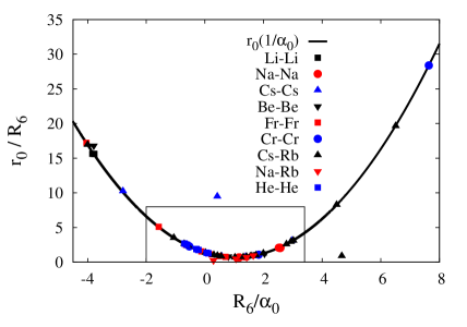
Figure 2: The VdW universal effective range in units of the VdW radius $R$ defined by $2\mu V(r)=-R^{4}/r^{6}$. Compared to several calculations 1996PhRvA..53..234C (Li-Li,Na-Na), 1994PhRvA..50.4827C (Na-Na), 1999PhRvA..59.1998F (Cs-Cs), 1994PhRvA..50.3177M (Cs-Cs), 2009EPJD…53…27O (Na-Rb), 2007JPhB…40.3497J (Be-Be), 2003JPhB…36.1085J (Cs-Rb), 2004PhRvA..69c0701P (Cr-Cr), 2004physics…6027K (Fr-Fr), 1986JPSJ…55..801K (H-H), 1992PhRvA..46.6956J (H-H), 2006EL…..76..582S (H-H), 1995PhRvA..51.2626J (H-H).

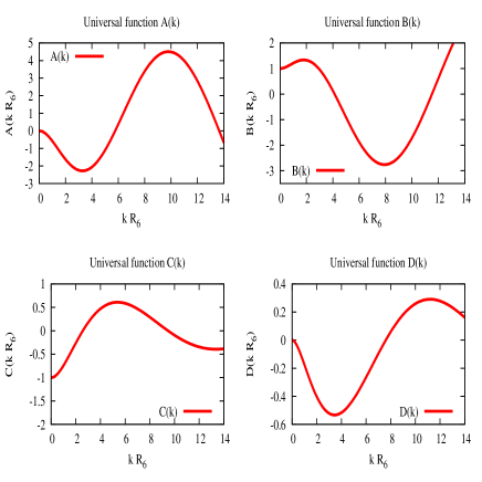
Figure 3: The VdW universal functions in units of the VdW radius $R$ defined by $2\mu V(r)=-R^{4}/r^{6}$. Using these functions one can determine the phase shift if the scattering length is known by the formula $k\cot\delta_{0}(k)=[\alpha_{0}{\cal A}(kR)+{\cal B}(kR)]/[\alpha_{0}{\cal C}(kR)+{\cal D}(kR)]$.

Figure 4: Convergence of the phase shift for a fixed momentum $k$ as a function of the short distance cut-off, $r_{c}$ in VdW units.

One important issue has to do with the cut-off dependence. From a Callan-Symanzik renormalization group type argument one has PavonValderrama:2007nu

$$\frac{d\delta(k,r_{c})}{d\,r_{c}}=-\,k^{3}\left(\frac{u_{k}(r_{c},r_{c})}{k}\right)^{2}$$ (33)

when $\alpha_{0}$ is fixed. This in turn means that for $U(r)\sim-R_{6}^{4}/r^{6}$ and using $u_{k}(r_{c},r_{c})/k\sim(r_{c}/R_{6})^{3/2}/k$ one has that finite cut-off corrections scale as

$$\delta(k)-\delta(k,r_{c})={\cal O}(k^{3}r_{c}^{4}/R_{6})$$ (34)

Thus, the short distance cut-off $r_{c}$ is a parameter for $kR_{6}\gg 1$ but becomes innocuous otherwise when $r_{c}\ll R_{6}$ implying that universality is robust. We show for a sample case in Fig. 4 the phase shifts for fixed energies, where the rather smooth converging pattern can be clearly confirmed.

Turning to the negative energy bound states with $E=-\hbar^{2}\gamma^{2}/(2\mu)$, the behaviour at long distances is

$$u_{\gamma}(r)\to Ae^{-\gamma r}$$ (35)

whereas at short distances the energy dependent boundary condition, Eq. (13) , holds. Orthogonality to the zero energy state requires that

$$\alpha_{0}=\frac{\int_{0}^{\infty}dr\,u_{\gamma}(r)u_{0,s}(r)}{\int_{0}^{\infty}dr\,u_{\gamma}(r)u_{0,c}(r)}\,.$$ (36)

This relation explicitly yields the scattering length from a given bound state. Inverting the formula we get, the energy spectrum, $E_{n}=-\hbar^{2}\gamma_{n}^{2}/2\mu$ for a fixed value of the scattering length and a fixed potential . This relation determines the energy spectrum $E_{n}$ from the scattering length $\alpha_{0}$ and the potential. Conversely, we can get the scattering length $\alpha_{0}$ from a given bound state wave number $\gamma$. In Fig. 5 we display the lowest bound states as functions of $\alpha_{0}$ for the pure VdW potential in scaled units. Such an universal plot allows also to deduce the scattering length from the knowledge of the weakly bound states in a complete model independent way.

Figure 5: Bound state spectrum for the VdW potential $R_{6}^{2}U(r)=-(R_{6}/r)^{6}[1+g(R_{6}/r)^{2}]$ for $g=0$ (solid), $g=0.1$ (long-dashed-dotted) )$,0.5$ (dashed) and $g=1$ (short-dashed-dotted). The horizontal line corresponds to a situation where $\alpha_{0}/R_{6}=0.336$ and the intersections to $\gamma_{n}$ values with $E_{n}=-\gamma_{n}^{2}/(2\mu)$.

We may ask how should the neglected higher order $1/r^{8}$ ,$1/r^{10}$, etc. terms in the potential affect the lowest order $1/r^{6}$ calculation. To this end we show in Fig. 6 the effect of adding the term $1/r^{8}$ to the potential, see Eq. (12), in the s-wave phase shift fixing the scattering length $\alpha_{0}$ to the same value. In view of the rather small $g_{1}\sim 10^{-2}$ values listed in table 1 we expect tiny corrections at even large energies $kR_{6}\sim 10$. This result not only shows a clear dominance of the leading dispersion coefficient $C_{6}$ but also that scaling of VdW forces holds beyond naive dimensional estimates, $kR_{6}\approx 1$. This raises the question on the usefulness of including higher order dispersion coefficients such as $C_{8}$ and $C_{10}$ since the region where they can distinctly be disentangled without entering the finite size regime is extremely narrow. This is also seen in the bound state spectrum displayed in Fig. 5 since for $\gamma R_{6}<10$ a rather tiny energy shift is observed in the closest states to the continuum.

Figure 6: s-wave phase shifts for the VdW potential $R_{6}^{2}U(r)=-(R_{6}/r)^{6}[1+g(R_{6}/r)^{2}]$ for $g=0,0.1,0.5,1.$ for a fixed sample value of the scattering length $\alpha_{0}/R_{6}=0.335$.

5 Phenomenological potentials

In our way of treating the renormalization of VdW forces, we need not specify the value of the scattering length, $\alpha_{0}$, since it exactly factors out in the expression for the phase shift (see Eq. (31)). However, to predict scattering phase shifts a particular value of $\alpha_{0}$ must be used. It is interesting to analyze the results from a comparative perspective with the so called realistic inter-atomic potential models, which aim at a description through the entire range of distances. Thus, one can deduce from those the value of the scattering length. The advantage of such potentials is that they provide a complete description of the interaction throughout the entire separation range. However, many of its features cannot be deduced accurately from first principles calculations. In contrast, the long range part of the interaction has a well accepted form in terms of a few parameters, say $C_{6}$, $C_{8}$, $C_{10}$ which, in principle, can be evaluated from ab initio atomic structure electronic wave functions.

Most modern inter-atomic potentials include the asymptotic Van der Waals long distance behaviour. They are generally written as the sum of a long range dispersive term and a short distance term with a core which reflects the impenetrability of two atoms. To keep the discussion as simple as possible in terms of the number of parameters, and for illustration purposes, we will analyze the venerable Lennard-Jones potential, which we write as

$$2\mu V_{\rm L.J.}=U_{LJ}(r)=\frac{1}{R_{6}^{2}}\left[g^{6}\left(\frac{R_{6}}{r}\right)^{12}-\left(\frac{R_{6}}{r}\right)^{6}\right]\,,$$ (37)

where we have chosen to scale the potential in the long distance VdW units $R=R_{6}=(2\mu C_{6})^{\frac{1}{4}}$. The value of the dimensionless constant $g$ determines the classical turning point $U_{\rm LJ}(gR_{6})=0$. In these form the minimum of the potential is at $r_{\rm min}=2^{\frac{1}{6}}R_{6}$ and $U_{\rm min}=-1/(4g^{6}R_{6}^{2})$. A relevant dimensionless parameter is the total number of bound states, which obviously increases as the repulsive term is shifted towards the origin. Within a WKB approximation the number of bound states is given by

$$N_{\rm WKB}=\frac{1}{\pi}\int_{a}^{\infty}dr\sqrt{-U_{\rm LJ}(r)}=\frac{0.1339}{g^{2}}\,,$$ (38)

where $a=gR_{6}$ is the zero energy classical turning point. For $g=0.0365$ we get $N_{\rm WKB}=100$, for $g=0.0517491$ we get $N_{\rm WKB}=50$ and for $g=0.115715$ we get $N_{\rm WKB}=10$.

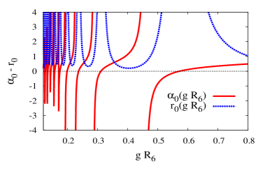
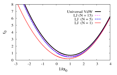
Figure 7: (Upper panel) The scattering length $\alpha_{0}$ and effective range $r_{0}$ of the Lennard-Jones potential as a function of the zero energy turning point $gR_{6}$ (in VdW units). (Lower panel) The effective range $r_{0}$ of the Lennard-Jones model as a function of the inverse scattering length $1/\alpha_{0}$ compared to the universal renormalized VdW formula (in VdW units) for different number of bound states $N=1,5,15$.

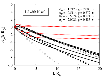
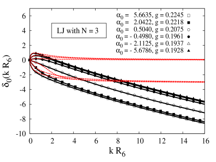
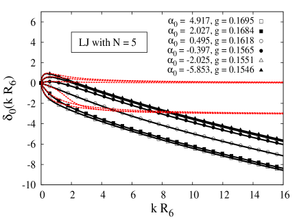
Figure 8: The Lennard-Jones s-wave phase shifts $\delta_{0}(k)$ (in radians) for different number of bound states $N=0,1,3,5$ as a function of the wave number (points) compared with the corresponding VdW renormalized ones having the same scattering length $\alpha_{0}$ (solid). We compare also with the effective range expansion truncated to second order $k\cot\delta_{0}(k)=-1/\alpha_{0}+r_{0}k^{2}/2$ (dots).

Using the VdW scaled units one can predict the scattering length $\alpha_{0}$ from the LJ potential and the phase shifts unambiguously for any value of $g$. The result is displayed in Fig. 7. According to Levinson’s theorem any time the scattering length jumps from $-\infty$ to $+\infty$ a new bound state dives from the continuum into the negative energy spectrum. In Fig. 7 we display the effective range as given by Eq. (17). The divergent values of $r_{0}$ correspond, according to our low energy theorem, to points where the scattering length goes through zero. The very strong sensitivity to the precise location of the position of the core is manifest. In Fig. 7 we compare the universal and renormalized VdW effective range formula with the actual values deduced from the Lennard-Jones potential for a different number of bound states $N=1,5,15$ (plus or minus one). The minima in the curve corresponds to a value of the scattering length passing from $-\infty$ to $+\infty$ which corresponds to entering a new bound state in the spectrum. As one sees in the LJ case there is a multivalued function reflecting the multiple branches already observed in Fig. 7. The rather universal pattern of this figure is striking because it explicitly shows that to very small uncertainties the value of the scattering length largely determines the value of the effective range, regardless on the precise number of bound states. The only remarkable exception corresponds to the case with no bound states where the zero energy turning point is located at increasingly large distances.

In a sense these correspond to almost low energy identical situations, where additional bound states are hosted by the potential as the short range repulsion is displaced towards the origin. Moreover, one expects that the largest discrepancies from renormalized VdW and LJ should take place in the case of large scattering lengths, since a larger sensitivity to short distances is displayed in such a case. Actually, this is what happens. We note that there is a relatively constant shift between $r_{0}^{\rm LJ}$ and $r_{0}^{\rm VdW}$ of about $0.5-1.0$ for $|\alpha_{0}|>10R_{6}$. However, the renormalized theory works better the larger the number of bound states and also for small scattering lengths, since as we discussed in the previous section for $\alpha_{0}\gg R_{6}$ large distances dominate. A relevant question is whether renormalization theory as explained above can account for the behaviour of the phase shifts in a energy region where the De Broglie wavelength is larger than the short distance $kR_{6}g\ll 1$ provided the scattering length $\alpha_{0}$ is the same. The result is shown in Fig. 8 for a variety of values of $g$ which cover several cases with large and small scattering lengths as compared to the VdW radius. We see the anticipated similarity despite the fact that both potentials are completely different at short distances. Actually, the phase-shifts are indistinguishable for $kR_{6}\ll 1$, but they go hand in hand far beyond this expected region; what matters is $kR_{6}g\ll 1$. On the other hand, the ERE given by Eq. (15) truncated to second order, i.e. taking $v_{2}=0$ only works for $kR_{6}\ll 1$. In a sense this is equivalent to “seeing” the Van der Waals force in a scattering experiment. The point of renormalization theory is that it yields model independent results and hence any discrepancy with data can be clearly attributed to a deficient incorporation of the long distance physics.

6 The Effective Field Theory and its limits

At very low energies the interaction between neutral atoms can be handled by an effective range expansion, Eq. (15), where the long range character of the VdW potential becomes manifest in the third term of the expansion. However, if only the first two terms are retained

$$k\cot\delta_{0}(k)=-\frac{1}{\alpha_{0}}+\frac{1}{2}r_{0}k^{2}\,,$$ (39)

there arises the interesting possibility of universally representing long range forces on equal footing with short range interactions. We may judge the quality of such an appealing approximation by comparing Fig. 8 the result of the renormalized VdW theory with the ERE. As we see the expansion truncated to second order breaks down at low energies, namely $kR_{6}\ll 1$, as expected.

Under these very restrictive conditions the problem can be advantageously treated by using EFT methods, which are based on the compelling idea that at such long wavelengths atoms behave as elementary structureless particles. This point of view has been stressed recently (see e.g. Braaten:2004rn ; Braaten:2007nq ) with particular fruitful predictions in the three-body problem Braaten:2006vd ; Platter:2009gz where Efimov states have been predicted. This is usually done by considering the Lagrangian density

$${\cal L}(x)=\psi^{\dagger}(x)\left[i\partial_{t}+\frac{\nabla^{2}}{2m}\right]\psi(x)$$ (40)

$$- \frac{1}{2}\int d^{3}x^{\prime}\psi^{\dagger}(x)\psi^{\dagger}(x^{\prime})V(\vec{x}-\vec{x}^{\prime})\psi(x^{\prime})\psi(x)\,,$$

where $\psi(x)\equiv\psi(\vec{x},t)$ are space-time canonically quantized fields with Fermi or Boson statistics depending upon the spin nature of the atom as a whole. The irreducible two-point function is the potential $V(\vec{x})$ which is taken as

$$\langle\vec{k}^{\prime}|V|\vec{k}\rangle\equiv\int d^{3}xe^{i(\vec{k}-\vec{k}^{\prime})\cdot\vec{x}}V(\vec{x})=C_{0}+C_{2}(\vec{k}^{\prime 2}+\vec{k}^{2})$$ (41)

Usually the coefficients $C_{0}$ and $C_{2}$ are assumed to be completely arbitrary. The corresponding Lippmann-Schwinger equation can be solved requiring introducing a momentum space cut-off $\Lambda$ (see e.g. Ref. Entem:2007jg and references therein)

$$-\frac{1}{\alpha_{0}} = \frac{10(C_{2}M\Lambda^{3}-3)^{2}}{9M\pi(-C_{2}^{2}M\Lambda^{5}+5C_{0})}-\frac{2\Lambda}{\pi}\,,$$ (42)

$$\frac{1}{2}r_{0} = \frac{50C_{2}\left(3+C_{2}M\Lambda^{3}\right)^{2}\left(6+C_{2}M\Lambda^{3}\right)}{27\pi\left(-5C_{0}+C_{2}^{2}\Lambda^{5}M\right)^{2}}+\frac{2}{\pi\Lambda}\,.$$ (43)

This leads for any cut-off $\Lambda$ to the mapping $(\alpha_{0},r_{0})\to(C_{0},C_{2})$. Eliminating $C_{0}$ and $C_{2}$ in favour of $\alpha_{0}$ and $r_{0}$, the phase shift becomes

$$p\cot\delta(p) = -\frac{2\Lambda}{\pi\alpha_{0}}\frac{(\pi-2\Lambda\alpha_{0})^{2}}{2\Lambda(\pi-2\Lambda\alpha_{0})+\alpha_{0}p^{2}(r_{0}\pi\Lambda-4)}$$ (44)

$$- \frac{2\Lambda}{\pi}+\frac{p}{\pi}\log\frac{\Lambda+p}{\Lambda-p}\,,$$

which is a real quantity for $p<\Lambda$, meaning that two-body unitarity is fulfilled. However, one has complex solutions for $C_{0}$ and $C_{2}$ if

$$\alpha_{0}^{2}r_{0}\pi\Lambda^{3}-16\alpha_{0}^{2}\Lambda^{2}+12\alpha_{0}\pi\Lambda-3\pi^{2}\leq 0\,.$$ (45)

which means that the effective Lagrangian, Eq. (40), becomes non hermitian ${\cal L}^{\dagger}(x)\neq{\cal L}(x)$. On the other hand, it is well known that three-body unitarity rests on off-shell two-body unitarity PhysRev.135.B1225 , a condition which cannot be met if the interaction is not hermitian, mainly because Schwartz’s principle. So the lesson is that while a complex two-body potential may fulfill on-shell two-body unitarity, a violation of three body unitarity is still possible Entem:2007jg .

Generally, Eq. (45) imposes a limit on the maximum value of the cut-off $\Lambda$, but to find it we need to know both $\alpha_{0}$ and $r_{0}$. For our case of VdW interactions we have seen that the universal formula for $r_{0}$ in terms of $\alpha_{0}$, Eq. (32) works extremely well if we judge by Fig. 2. Thus, if we merge Eq. (45) equal to null and Eq. (32) we obtain a boundary in the $(\Lambda,\alpha_{0})$ plane which is suitably represented in Fig. 9. Essentially and up to minor variations the meaning is that the cut-off $\Lambda$ cannot exceed the VdW wave number, $\Lambda<\pi/(2R_{6})$. This issue is relevant for three-body calculations Platter:2006ev ; Platter:2008cx as addressed recently Canham:2009xg .

The analysis of the problem in coordinate space assuming an effective local and energy independent long distance dynamics and an energy dependent boundary condition at short distances have been analyzed in Ref. PavonValderrama:2005wv for s-waves and in Ref. Cordon:2009pj in the three-dimensional case. It is found that the locality condition for an s-wave implies

$$\frac{d}{dk^{2}}\left[\frac{u_{k,{\rm S}}^{\prime}(r_{c})}{u_{k,{\rm S}}(r_{c})}\right]=-\frac{\int_{0}^{r_{c}}u_{k,{\rm S}}(r)^{2}dr}{u_{k,{\rm S}}(r_{c})^{2}}\leq 0$$ (46)

where $u_{k,{\rm S}}(r)$ is the wave function for $r\leq r_{c}$. Note the resemblance with Eq. (10). If there would be no interaction for $r>r_{c}$ then we have

$$u_{k}(r)=\sin\left(kr+\delta_{0}(k)\right)\,,\quad r>r_{c}\,,$$ (47)

which can be matched to the inner $r<r_{c}$ region yielding

$$\frac{d}{dk^{2}}\left[k\cot\left(kr_{c}+\delta_{0}(k)\right)\right]\leq 0\,,$$ (48)

this is equivalent to Wigner’s causality condition Wigner:1955zz , as noted in Phillips:1996ae , and combined to the ERE, Eq. (39), provides a constraint on the effective range

$$r_{0}/(2r_{c})\leq 1-r_{c}/\alpha_{0}+r_{c}^{2}/(3\alpha_{0}^{2})\,.$$ (49)

If there is no potential for $r>r_{c}$ and take $r_{0}=r_{\rm VdW}$ we get a universal lower limit for $r_{c}$. A similar conclusion has been presented recently Hammer:2009zh . The conditions featuring causality in coordinate space as well as off-shell unitarity in momentum space are depicted in Fig. 9, and suggest that modelling a finite range of VdW forces by an effective Lagrangian such as Eq. (40) requires assuming a cut-off distance larger than the VdW length.

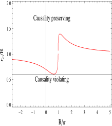
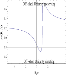
Figure 9: Boundaries on the cut-off for Van der Waals systems with reduced potential $2\mu V(r)=-R^{4}/r^{6}$ for which causality in coordinate space (left panel) and off-shell unitarity in momentum space (right panel) is preserved.

7 Conclusions

Renormalization ideas can profitably be exploited in conjunction with the superposition principle of boundary conditions in the description of model independent and universal features of the VdW force. Our main points are

• Van der Waals interactions between neutral atoms obey scaling rules which allow to determine the scattering and binding properties universally. They are well satisfied phenomenologically and extend much beyond low energy approximations such as the effective range expansion.

• There is a clear dominance of the leading $C_{6}$ contribution in a rather wide energy range. The range where higher order corrections due to $C_{8}$ or $C_{10}$ provide a distinct correction yet the finite size effects can still be neglected is extremely narrow or inexistent.

• Van der Waals potentials can be represented by short distance contact interactions under restrictive conditions based on causality and off-shell unitarity which are independent on the value of the scattering length. It is inconsistent to model VdW forces assuming a cut-off distance smaller than the VdW length.

We thank M. Pavón Valderrama and R. González Férez for discussions. Work supported by Spanish DGI and FEDER funds with grant FIS2008-01143, Junta de Andalucía grant FQM-225-05, EU Integrated Infrastructure Initiative Hadron Physics Project contract RII3-CT-2004-506078.

References

- (1) J.S. Rowlinson, Cohesion (Cambridge University Press, 2005).
- (2) F. London, Zeitschrift fur Physik 63 (1930) 245.
- (3) H.B.G. Casimir and D. Polder, Phys. Rev. 73 (1948) 360.
- (4) G. Feinberg and J. Sucher, Phys. Rev. A2 (1970) 2395.
- (5) G. Feinberg, J. Sucher and C.K. Au, Phys. Rept. 180 (1989) 83.
- (6) K.M. Case, Phys. Rev. 80 (1950) 797.
- (7) W. Frank, D.J. Land and R.M. Spector, Rev. Mod. Phys. 43 (1971) 36.
- (8) J. Weiner, Cold and Ultracold Collisions in Quantum Microscopic and Mesoscopic Systems (Cambridge University Press, 2004).
- (9) G.F. Gribakin and V.V. Flambaum, Phys. Rev. A 48 (1993) 546.
- (10) B. Gao, Phys. Rev. A58 (1998) 1728.
- (11) V.V. Flambaum, G.F. Gribakin and C. Harabati, Phys. Rev. A 59 (1999) 1998.
- (12) B. Gao, Phys. Rev. A 80 (2009) 012702.
- (13) A. Calle Cordon and E. Ruiz Arriola, (2009), 0912.1714[cond-mat.other].
- (14) E. Braaten and H.W. Hammer, Phys. Rept. 428 (2006) 259, cond-mat/0410417.
- (15) E. Braaten, M. Kusunoki and D. Zhang, Annals Phys. 323 (2008) 1770, 0709.0499.
- (16) L. Platter, Few Body Syst. 46 (2009) 139, 0904.2227.
- (17) I.N. Levine, Quantum Chemistry (Allyn and Bacon, 1974).
- (18) W. Heitler and F. London, Zeitschrift fur Physik 44 (1927) 455.
- (19) W. Kolos and C.C. Roothaan, Reviews of Modern Physics 32 (1960) 219.
- (20) R. Eisenschitz and F. London, Zeitschrift fur Physik 60 (1930) 491.
- (21) A. Calle Cordón, Renormalización de Interacciones Atómicas mediante condiciones de contorno (Master Thesis (University of Granada) December, 2007).
- (22) J. Mitroy and M.W.J. Bromley, Phys. Rev. A 71 (2005) 032709, arXiv:physics/0411172.
- (23) E.H. Lieb and W.E. Thirring, Phys. Rev. A 34 (1986) 40.
- (24) K. Cahill and V.A. Parsegian, eprint arXiv:q-bio/0312005 (2003), arXiv:q-bio/0312005.
- (25) A.M. Lane and R.G. Thomas, Rev. Mod. Phys. 30 (1958) 257.
- (26) M. Pavon Valderrama and E.R. Arriola, Phys. Rev. C74 (2006) 054001, nucl-th/0506047.
- (27) M. Pavon Valderrama and E.R. Arriola, Annals Phys. 323 (2008) 1037, 0705.2952.
- (28) E. Ruiz Arriola, A. Calle Cordon and M. Pavon Valderrama, (2007), 0710.2770.
- (29) S.V. Khristenko, A.I. Maslov and V.P. Shevelko, Molecules and Their Spectroscopic Properties (Springer Series on Atoms and Plasmas. Vol. 21. Springer-Verlag, 1998).
- (30) Z. Yan et al., Phys. Rev. A 54 (1996) 2824.
- (31) A. Derevianko, J.F. Babb and A. Dalgarno, Phys. Rev. A 63 (2001) 052704, arXiv:physics/0102030.
- (32) S.G. Porsev and A. Derevianko, Jour. Chem. Phys. 119 (2003) 844, arXiv:physics/0303048.
- (33) M. Marinescu, D. Vrinceanu and H.R. Sadeghpour, Phys. Rev. A 58 (1998) 4259.
- (34) S.G. Porsev and A. Derevianko, Soviet Journal of Experimental and Theoretical Physics 102 (2006) 195.
- (35) J. Werner et al., Physical Review Letters 94 (2005) 183201, arXiv:cond-mat/0412049.
- (36) B.R. Levy and J.B. Keller, Journal of Mathematical Physics 4 (1963) 54.
- (37) R. Côté, E.J. Heller and A. Dalgarno, Phys. Rev. A 53 (1996) 234.
- (38) R. Côté and A. Dalgarno, Phys. Rev. A 50 (1994) 4827.
- (39) V.V. Flambaum, G.F. Gribakin and C. Harabati, Phys. Rev. A 59 (1999) 1998.
- (40) M. Marinescu, Phys. Rev. A 50 (1994) 3177.
- (41) H. Ouerdane and M.J. Jamieson, European Physical Journal D 53 (2009) 27, 0802.1222.
- (42) M.J. Jamieson et al., Journal of Physics B Atomic Molecular Physics 40 (2007) 3497.
- (43) M.J. Jamieson et al., Journal of Physics B Atomic Molecular Physics 36 (2003) 1085.
- (44) Z. Pavlović et al., Phys. Rev. A 69 (2004) 030701, arXiv:physics/0309076.
- (45) M. Kemal Öztürk and S. Özçelik, ArXiv Physics e-prints (2004), arXiv:physics/0406027.
- (46) N. Koyama and J.C. Baird, Journal of the Physical Society of Japan 55 (1986) 801.
- (47) M.J. Jamieson, A. Dalgarno and J.N. Yukich, Phys. Rev. A 46 (1992) 6956.
- (48) A. Sen, S. Chakraborty and A.S. Ghosh, Europhysics Letters 76 (2006) 582.
- (49) M.J. Jamieson, A. Dalgarno and M. Kimura, Phys. Rev. A 51 (1995) 2626.
- (50) E. Braaten and H.W. Hammer, Annals Phys. 322 (2007) 120, cond-mat/0612123.
- (51) D.R. Entem et al., Phys. Rev. C77 (2008) 044006, 0709.2770.
- (52) C. Lovelace, Phys. Rev. 135 (1964) B1225.
- (53) L. Platter and D.R. Phillips, Few Body Syst. 40 (2006) 35, cond-mat/0604255.
- (54) L. Platter, C. Ji and D.R. Phillips, Phys. Rev. A79 (2009) 022702, 0808.1230.
- (55) D.L. Canham and H.W. Hammer, (2009), 0911.3238.
- (56) A. Calle Cordon and E. Ruiz Arriola, (2009), 0905.4933[nucl-th].
- (57) E.P. Wigner, Phys. Rev. 98 (1955) 145.
- (58) D.R. Phillips and T.D. Cohen, Phys. Lett. B390 (1997) 7, nucl-th/9607048.
- (59) H.W. Hammer and D. Lee, Phys. Lett. B681 (2009) 500, 0907.1763.