Existence and stability of viscous shock profiles for 2-D isentropic MHD with infinite electrical resistivity
Abstract.
For the two-dimensional Navier–Stokes equations of isentropic magnetohydrodynamics (MHD) with -law gas equation of state, , and infinite electrical resistivity, we carry out a global analysis categorizing all possible viscous shock profiles. Precisely, we show that the phase portrait of the traveling-wave ODE generically consists of either two rest points connected by a viscous Lax profile, or else four rest points, two saddles and two nodes. In the latter configuration, which rest points are connected by profiles depends on the ratio of viscosities, and can involve Lax, overcompressive, or undercompressive shock profiles. For the monatomic and diatomic cases and , with standard viscosity ratio for a nonmagnetic gas, we find numerically that the the nodes are connected by a family of overcompressive profiles bounded by Lax profiles connecting saddles to nodes, with no undercompressive shocks occurring. We carry out a systematic numerical Evans function analysis indicating that all of these two-dimensional shock profiles are linearly and nonlinearly stable, both with respect to two- and three-dimensional perturbations. For the same gas constants, but different viscosity ratios, we investigate also cases for which undercompressive shocks appear; these are seen numerically to be stable as well.
1. Introduction
In this paper, we continue the investigations of [GZ, ZH, MaZ3, MaZ4, Ra, RZ, Z5, TZ, BeSZ, Br1, Br2, BrZ, HuZ2, BHRZ, HLZ, HLyZ1, HLyZ2, BHZ] on stability and dynamics of large-amplitude viscous shock profiles, examining classical Lax-type and nonclassical overcompressive and undercompressive shocks occurring in isentropic magnetohydrodynamics (MHD) with infinite electrical resistivity.
Existence of large-amplitude profiles for full (nonisentropic) magnetodydrodynamics was studied in pioneering works of Germain and Conley–Smoller [G, CS1, CS2], making use of properties of the traveling-wave ODE as a gradient system and of Conley index techniques. Further investigations have been carried out by Freistühler–Szmolyan [FS] using geometric singular perturbation techniques and by Freistühler–Roehde [FR1, FR2] using a combination of bifurcation analysis and numerical approximation. In this generality, the traveling-wave ODE for MHD profiles is a six-variable dynamical system, with up to four rest points corresponding to endstates of various inviscid shock waves. For an ideal gas law, it is known that fast and slow Lax shocks always possess a viscous profile. In certain special cases, or in certain limiting ratios of viscosity, heat conduction, etc., it is known that intermediate shocks do or do not possess profiles; however, in general, the profile existence problem for the full nonisentropic case is accessible at present only numerically. For further discussion, see [FS, FR1, FR2] and references therein.
In the present work, we examine in detail the restricted case of isentropic flow with infinite electrical resistivity, in two dimensions, for which the traveling-wave ODE becomes a planar dynamical system. This example exhibits the main features of the general case, in a simpler setting conducive to systematic numerical investigation.
Specifically, for a rather general equation of state (convex, decreasing in specific volume, and blowing up at least linearly with density as density goes to infinity) we show in Sections 2.43 and (4.1) that the phase portrait of the traveling-wave ODE generically consists of either two rest points connected by a viscous Lax profile, or else four rest points, two saddles and two nodes. In the latter, four rest point configuration, the Lax shocks involving consecutive rest points ordered by specific volume always have connecting profiles. The remaining, “intermediate” shocks may or may not admit profiles, depending on the ratio of parallel to transverse viscosity. Specifically, we show in Section 4.3 by phase plane (and, separately, by singular perturbation) analysis that, similarly as in the nonisentropic case [FS, G], any intermediate shock with decreasing specific volume permits a connection for some viscosity ratios and not for others. By entropy considerations, shocks with increasing specific volume never have connecting profiles. Here, and elsewhere, we without loss of generality restrict discussion to the case of a left-moving shock. (For right-going shocks, the ordering would be reversed.)
We supplement this abstract existence discussion by a systematic numerical existence study for specific parameter values in physical range. For the most common cases of monatomic or diatomic gas, or , with standard viscosity ratio for a nonmagnetic gas (see (2.3)), we find that there occurs only one profile configuration, with the nodes connected by a family of overcompressive profiles (intermediate shocks) bounded by Lax profiles connecting saddles to nodes in a four-sided configuration (one pair of opposing sides corresponding to slow and fast Lax connections, the other to intermediate Lax connections). Undercompressive profiles do not seem to occur in this parameter range.
Next, restricting to the same parameters , and standard viscosity ratio, we carry out numerically a systematic stability analysis of these waves, using the general numerical Evans function techniques developed in [Br2, BrZ, HuZ2, HLZ, HLyZ1, HLyZ2, BHZ, Z5]. Our results, carried out up to extremely high Mach number (typically Mach , but in some cases up to Mach ), indicate that all of the above profiles, both Lax- and overcompressive type, are spectrally stable in the generalized Evans function sense defined in [ZH, MaZ3], both with respect to two-dimensional and three-dimensional perturbations. These results are described in Sections 5 and 7. By the abstract framework established in [MaZ3, MaZ4, Z1, Ra, RZ], this implies linearized and nonlinear time-asymptotic orbital stability, as described for completeness in Section 2.5. Varying the viscosity ratio, we carry out case studies also for examples of undercompressive profiles. Numerically, these are seen to be (Evans, hence linearly and nonlinearly) stable as well.
Finally, in Section 8 we discuss our results and suggest directions for further study.
2. Preliminaries
2.1. Equations and assumptions
In Lagrangian coordinates, the equations for compressible isentropic magnetohydrodynamics (MHD) take the form
| (2.1) |
where denotes specific volume, velocity, pressure, magnetic induction, constant, and and the two coefficients of viscosity, the magnetic permeability, and the electrical resistivity; see [A, C, J] for further discussion.
We restrict mainly to the case of an ideal polytropic gas, in which case the pressure function takes form
| (2.2) |
where and are constants that characterize the gas, the limiting case corresponding to the barotropic, or constant-temperature approximation and corresponding to the isentropic, or constant-entropy approximation, of the ideal pressure law . Though we do not specify , we have in mind mainly the ratio
| (2.3) |
typically prescribed for (nonmagnetic) gas dynamics [Ba]. (By rescaling space and time, we can rescale all transport coefficients by a common factor; the ratio , however, is invariant.)
In the thermodynamical rarified gas approximation, is the average over constituent particles of , where is the number of internal degrees of freedom of an individual particle, or, for molecules with “tree” (as opposed to ring, or other more complicated) structure,
| (2.4) |
where is the number of constituent atoms [Ba]: for monatomic, for diatomic gas.
An interesting subcase is the limit of infinite electrical resistivity , in which the last two equations of (2.1) are replaced by
| (2.5) |
and only the velocity variables experience parabolic smoothing, through viscosity. We can restrict further to the two-dimensional case, setting and dropping these variables from consideration, as we shall do for most of our investigations.
2.1.1. Eigenvalues of the -d inviscid system
The inviscid version of system (2.1) in dimension two, is, introducing the scalar quantities , ,
| (2.6) |
or, in quasilinear form,
| (2.7) |
where . This system has four eigenvalues of the form , where are the roots of
| (2.8) |
As the discriminant of (2.8) is positive for , the two roots and are positive real, verifying hyperbolicity. When , the discriminant can be zero for . We do not explicitly require this computation in our analysis, but include it for general interest/orientation.
2.2. Viscous shock profiles and the rescaled equations
A viscous shock profile of (2.1) is a traveling-wave solution,
| (2.9) |
moving with speed and connecting constant states
| (2.10) |
Such a solution is a stationary solution of the system of PDEs
| (2.11) |
where we have denoted , , i.e., a solution of the system of ODEs
| (2.12) |
Integrating, we obtain
| (2.13) |
for some constants of integration .
For fixed , the rest points of (2.13) comprise the possible endstates that can be connected by a viscous profile with speed , which necessarily satisfy the Rankine–Hugoniot conditions
| (2.14) | ||||
determining pairs of states connected by an inviscid shock wave, where
denotes jump in the quantity across the shock.
2.2.1. Rescaled evolution equations
2.2.2. Rescaled profile equations
Viscous shock profiles of (2.16) must satisfy the system of ordinary differential equations
| (2.17) |
together with the boundary conditions
Evidently, we can integrate each of the differential equations from to , and using the boundary conditions (in particular and ), we find, after some elementary manipulations, the profile equations (after having introduced shorthand notation , , ):
| (2.18) | ||||
| (2.19) | ||||
| (2.20) |
with .
2.2.3. The case
2.3. The profile ODE as generalized gradient flow
We now recall the general fact [G, CS1, CS2, FR1, FR2] concerning a hyperbolic–parabolic conservation law
| (2.23) |
, possessing a convex entropy/entropy flux pair
that is viscosity-compatible in the sense that
| (2.24) |
that the associated traveling wave ODE
| (2.25) |
may be written always in the form of a generalized gradient flow
| (2.26) |
serving to increase in the direction of positive . Here,
| (2.27) |
so that
| (2.28) |
by direct computation. Likewise, by (2.24). We will refer to potential as the relative entropy (more properly speaking, entropy production).
Remark 2.1.
Evidently, rest points of the traveling-wave ODE correspond to critical points of the relative entropy. At a rest point , the Hessian is given by
| (2.29) |
so that, in particular, . This gives a connection between the number of positive and negative characteristics and the type of the critical point of .
2.3.1. Reduced gradient flow
Using the assumed structure that has constant left kernel, (2.23), as is often the case in applications, we may make a further simplification by the use of entropy coordinates. Introducing the entropy variable
| (2.30) |
globally invertible, by , and noting that , we obtain from (2.26) the more useful version
| (2.31) |
| (2.32) |
where the block-diagonal form of follows from vanishing of the first row (inherited from left factor ) and compatibility assumption (2.24), which implies also .
Make, finally, the standard assumption (see, e.g., [MaZ3, Z1, Z2]) that relation
| (2.33) |
coming from the traveling-wave ODE may be solved for as a function of , i.e.
| (2.34) |
Then, defining the reduced potential
| (2.35) |
and noting from (2.32) that for , we obtain the relations
| (2.36) |
and
| (2.37) |
expressing (2.25) as a reduced generalized gradient flow in the parabolic entropy coordinates alone. We remark in passing that this implies that is strictly increasing in positive and not only nondecreasing as shown above. Moreover, we may find directly from (2.36) without computing either the full potential or the entropy flux , which in practice is a great simplification.
Remark 2.2.
In particular, if there is a viscous profile connecting , we have
| (2.38) |
2.3.2. Application to MHD
For MHD, we have a viscosity-compatible convex entropy
associated with entropy variables and denoting by and as in (2.1).111 See [Kaw] for related computations in the nonisentropic case. The associated flux is . The entropy variable is thus
of which the parabolic coordinates are , exactly the ones appearing already in (2.18)–(2.20). The corresponding flux density, though we do not need it, is .
Substituting into (2.36) the relation obtained by integrating the -equation in the traveling-wave ODE, we obtain
| (2.39) |
which readily yields
| (2.40) | ||||
One checks that , , and .
2.3.3. The case
Substituting into (2.36) (2.40) the relation obtained by integrating the -equation in the traveling-wave ODE, and the relation obtained by integrating the -equation, we obtain, denoting ,
| (2.41) |
which readily yields
| (2.42) |
Alternatively, this may be obtained from the definition, substituting into (2.40) the value for ; however, we wish to point out the simplification afforded by working with the reduced problem, that is, to emphasize that one need not solve for in order to find , or for in order to find .
Remark 2.3.
Note that in the above we did not need to compute or even , but only to know the entropy variable , in order to determine the reduced potential by integration of (2.36). Likewise, computing the full potential by integration of (2.32), we obtain
where satisfies , hence , or
in agreement up to constant of integration with the formula obtained by direct substitution of and into (2.27). A further substitution yields
directly verifying the relation .
2.4. Types of shocks vs. connections
Consider a general system of conservation laws
as in (2.23). Inviscid shock waves correspond to triples satisfying the Rankine–Hugoniot conditions
| (2.43) |
where denotes the jump in quantity across the shock. The type of the shock wave is defined by the degree of compressivity
| (2.44) |
measuring the number of incoming characteristic modes relative to the shock, where and denote unstable and stable subspaces of a matrix , with corresponding to the classical Lax type, nonclassical overcompressive type, and corresponding to nonclassical undercompressive type. See [ZH, MaZ3, Z1] for further discussion.
At a slightly more detailed level, we define a - shock as a shock for which and are the indices of the largest positive characteristic speed at and the smallest negative characteristic speed at , where denote the eigenvalues of . Lax shocks are associated with a single characteristic family , and we refer to them simply as Lax -shocks. For overcompressive shocks, , and for undercompressive shocks, , with the degree of compressivity measuring the difference between and .
Now suppose (as in the present case) that has a constant left kernel and constant rank, without loss of generality
| (2.45) |
and that, if we denote by the Jacobian matrix of the flux ,
| (2.46) |
(In the case that there exist a viscosity compatible convex entropy, it may be checked [MaZ3] that necessarily has real eigenvalues, and is equivalent to (2.34).) It follows that traveling wave ODE (2.25) can be expressed as a nondegenerate reduced ODE on a manifold of dimension ; in the case that there exist a compatible convex entropy, it can simply be expressed as the reduced ODE (2.37) in .
Suppose further that the shock is noncharacteristic,
| (2.47) |
and the endstates satisfy the dissipativity condition
| (2.48) |
where, here and elsewhere, denotes spectrum of a matrix or linearized operator . In the case that there exist a viscosity-compatible convex entropy in the vicinity of , (2.48) is equivalent to the genuine coupling condition of Kawashima [Kaw] that no eigenvector of lie in the kernel of , and likewise for and .
All of these assumptions are satisfied quite generally in applications, in particular for the equations of isentropic or nonisentropic MHD with ideal pressure law. See [MaZ4, Z1, GMWZ1, GMWZ2] for further discussion and examples.
Lemma 2.4 ([MaZ3]).
Proof.
Block matrix reduction and standard invariant manifold theory; see Appendix A, [MaZ3]. ∎
Denoting by the dimension of the stable manifold of the -dimensional reduced ODE at the rest point corresponding to and by the dimension of the unstable manifold at the rest point corresponding to , define the connection number
| (2.50) |
measuring the type of the potential connection between rest points as a connecting orbit of the reduced ODE. Then, we have the following fundamental relation, generalizing the corresponding observation of [MP] in the strictly parabolic case.
Lemma 2.5 ([MaZ3]).
Proof.
Results (2.51)–(2.52) are obtained in [MaZ3] under the additional assumption that there exist a connecting profile. However, the proof uses existence only to conclude via homotopy that the number of positive eigenvalues of is the same at as at , under the weaker assumption that have real nonvanishing eigenvalues only along the profile. Under our global assumption on , we have the same conclusions also in the absence of a profile. ∎
That is, the type of the inviscid shock wave determines the type of the potential connection. In the simple, planar setting (2.22) of the case, we have the simple relation that Lax shocks correspond to saddle–node connections, overcompressive shocks to repellor–attractor connections, and undercompressive shocks to saddle–saddle connections.
An important consequence is that viscous profiles associated with Lax or undercompressive shocks are generically unique up to translation, while profiles associated with overcompressive shocks generically appear as part of an -parameter family (counting translations).
2.4.1. Type and orientation
We point out in passing a similar reduction principle at the level of the Rankine–Hugoniot equations, this time measuring the parity of , or equivalently the orientation of roots of the Rankine–Hugoniot relations. It is sometimes the case that certain of the Rankine–Hugoniot equations (2.43) can be solved for certain variables in terms of others, that is, without loss of generality, after relabeling , , that is invertible, so that . In this case, (2.43) reduces to
| (2.53) |
In the present case of isentropic MHD, we will reduce to a scalar equation in the specific volume .
Evidently, we have in this case whence, since is real and nonvanishing by assumption,
| (2.54) |
That is, the orientation of zeros of the full Rankine–Hugoniot relations is determined by the orientation of zeros of the reduced Rankine–Hugoniot relations (2.53). We make use of this later to help determine the types of rest points by consideration of a scalar reduced relation. Similar reasoning is used in [FR1] for a planar reduced relation, looking at orientations of intersections of nullcline curves (equivalent to orientation of zeros of the planar reduced condition).
2.5. The Evans function and stability
We conclude these preliminaries by a brief discussion of stability of general traveling-wave profiles, as determined by an Evans function, or “generalized spectral stability” condition. Throughout this section, we make the general assumptions (2.45), (2.46), (2.47), (2.48) of [MaZ3, MaZ4, Z1], as hold in particular for the MHD equations studied here. We add to these the further assumption of symmetric-dissipative hyperbolic–parabolic form [Z1, Z2]:
(S) There exist coordinates for which (2.23) becomes , with symmetric positive definite and block-diagonal, symmetric and either negative or positive definite, and block-diagonal, with positive definite. (Here and elsewhere, denotes the symmetric part of a matrix or linear operator .)
This structure guarantees the minimal properties needed to carry out an analysis, in particular that the nonlinear equations be local well-posed and that the linearized equations generate a semigroup; see [Z2, GMWZ1, GMWZ2] for further discussion. It is implied by existence of a viscosity-compatible convex entropy together with the condition that , real and nonzero by assumption, be also strictly positive or strictly negative, a minimal further requirement since in most applications is a scalar multiple of the identity. In particular, (S) and all other hypotheses are satisfied for the equations of MHD with ideal gas equation of state [MaZ4, Z1] under the single condition (2.47) of noncharacteristicity.
Linearizing about a stationary wave of (2.23) (stationarity may always be achieved by a change to coordinates moving with the wave), we obtain linearized evolution equations
| (2.55) |
where and depend on , converging asymptotically to values , . By asymptotic convergence (2.49) and dissipativity, (2.48), we find from a standard result of Henry [He] equating essential spectrum of asymptotically constant coefficient operators to that of their limiting constant-coefficient operators, that
for some , where denotes essential spectrum (defined as the part of the spectrum not consisting of eigenvalues); see [AGJ, GZ, Z1]. Moreover, this bound is sharp; in particular, is in the limit of the essential spectrum. At the same time, is always an eigenvalue of , due to translational invariance of the underlying equations (2.23), with associated eigenfunction .
The fact that there is no gap between the spectrum of and the imaginary axis makes this a degenerate case for which linearized and nonlinear stability analysis is trickier than usual. In the standard case of a sectorial operator for which there exists a spectral gap, one may conclude bounded linear stability from the spectral stability conditions of (i) nonexistence of unstable eigenvalues , and (ii) semisimplicity of neutral eigenvalues ; indeed, these are necessary and sufficient. However, here we have a nonsectorial operator with no spectral gap. Moreover, for the eigenvalue embedded in the essential spectrum of , it is not clear even what is the meaning of semisimplicity; see discussions of [ZH, MaZ3, Z1, Z2].
Nonetheless, as shown in [GZ, ZH, MaZ3, MaZ4, Z1], one can extract a simple necessary and sufficient condition for stability analogous to (i)–(ii) in terms of the Evans function associated with , a Wronskian
| (2.56) |
defined in terms of analytically-chosen bases and of the manifolds of solutions decaying as and of the eigenvalue equations written as a first-order system
| (2.57) |
where is an augmented “phase variable” including and suitable derivatives. By standard considerations, this may be defined on the complement of ; a more detailed look shows that permits an analytic extension to the boundary of this set– in particular, to the nonstable complex half-plane . For details of this construction, see, e.g., [AGJ, GZ, Z1, HuZ2]; we give some further discussion also in Section 5 and Appendix D.
Evidently, away from the essential spectrum , the Evans function vanishes at if and only if is an eigenvalue of , corresponding to existence of a solution of the eigenvalue equations decaying at both . Indeed, the multiplicity of the root is equal to the multiplicity of the eigenvalue [GJ1, GJ2, MaZ3, Z1]. The meaning of the multiplicity of the root of at embedded eigenvalue is less obvious, but is always greater than or equal to the order of the embedded eigenvalue [MaZ3, Z1].
By the discussion in Section 2.4, in particular relation (2.51), a traveling-wave profile lies in an -parameter family of nearby solutions, where is (by dimensionality) at least , where is the degree of compressivity defined in (2.44), with equality in the case that the connection is a maximally transversal intersection of the unstable manifold at with the stable manifold at . Assume for simplicity the typical case that equality holds,
| (2.58) |
and the manifold of nearby solutions is smooth. Then, the stability condition is
(D) has precisely roots on the nonstable half-plane , necessarily at .
This is analogous to the stability condition in the standard sectorial case, with nonvanishing away from corresponding to the standard spectral condition (i), and vanishing to order at indicating that the multiplicity of this zero is accounted for entirely by genuine eigenfunctions corresponding to variations of the traveling wave connection along the -parameter family of nearby solutions, a generalized version of semi-simplicity [ZH, MaZ3, Z1].
2.5.1. Linear and nonlinear stability
We have the following basic results relating the Evans condition (D) to stability.
Proposition 2.6 ([MaZ3]).
Proposition 2.7 ([MaZ4, RZ]).
Under assumptions (2.45)–(2.48), (S), and definining as in (2.58), the Evans condition (D) implies, first, existence of a family of nearby solutions , , and, second, nonlinear time-asymptotic orbital stability, in the following sense: For any solution of (2.23) with initial difference sufficiently small and some uniform , exists for all , with
| (2.59) |
Moreover, there exist , such that
| (2.60) |
and
| (2.61) |
for all . (phase-asymptotic orbital stability).
A similar result holds in the mixed, under-overcompressive case that the family of nearby traveling waves has dimension different from (necessarily greater than) ; see [RZ].
2.5.2. The integrated Evans condition
Noting that is in divergence form, we may conclude for any that satisfaction of the eigenvalue ODE for an solution decaying exponentially in up to one derivative implies that is also bounded and exponentially decaying, and satisfies the integrated eigenvalue equation
| (2.62) |
where . Associated with is an integrated Evans function , which like may be defined analytically on the nonstable half-plane . This permits the following simplified stability condition, in practice easier to verify.
Proposition 2.8 ([ZH, MaZ3]).
Under assumptions (2.45)–(2.48), in the Lax or overcompressive case, the Evans condition (D) is equivalent to the integrated Evans condition
() is nonvanishing on the nonstable half-plane ,
and in the undercompressive case to
(’) has on the nonstable half-plane a single zero of multiplicity one at .
In the Lax and overcompressive cases that are the main focus of our investigation here, the change to integrated coordinates has the effect of removing the zeros of at the origin, making the Evans function easier to compute numerically and the Evans condition easier to verify.
3. Rankine-Hugoniot Conditions
The Rankine-Hugoniot conditions for isentropic MHD are, in the notation , , ,
| (3.1) | ||||
| (3.2) | ||||
| (3.3) | ||||
| (3.4) |
Under the scaling (2.15), we have , , and without loss of generality (by translation invariance), we may take , . Last, we may take without loss of generality (by rotational invariance) , whereupon we obtain from (3.3)–(3.4) that , which, so long as
| (3.5) |
gives, finally,
| (3.6) |
Collecting, we have the normalizations
| (3.7) |
To generate all possible shock profiles, up to invariances of the equations, we shall vary , , without loss of generality nonnegative, and , without loss of generality between and (since we can always arrange that correspond to the rest point with larger value), and solve for the remaining coordinates , , and the parameter appearing in the pressure law. Parameters that will be important in the whole study are
| (3.8) |
(Note that, under the rescaling that we used, , , in the original coordinates.)
Remark 3.1.
In the excluded case , profiles are prohibited by entropy consideration, (2.38).
Remark 3.2.
Note that it does not follow in general that or , but does follow when profiles are unique, i.e., in the Lax or undercompressive case, and one such profile is known to exist. (Recall the discussion of types of shocks and relation to uniqueness of profiles in Section 2.4).
Proposition 3.3.
Proof.
Remark 3.4.
So far, we have made no restriction on dimension or , so our analysis of the Rankine–Hugoniot conditions holds for the general three-dimensional isentropic case.
3.1. Global rest point configuration
Proposition 3.3 gives a convenient means for stepping through the possible shock connections, and is the main method we will use to generate shocks in our numerical investigations of shock stability. For the study of the existence problem it is more useful to take a global point of view, fixing a left state and speed in the unrescaled coordinates, and studying the configuration of rest points (possible right states) in the resulting traveling-wave ODE. In the rescaled coordinates, this amounts to fixing , , and , or, equivalently, the more convenient parameters , and solving for all possible .
Proposition 3.5.
In the parallel case , for and , there exists a unique parallel solution satisfying , with associated magnetic field . If is not between and , then these are the only rest points, with corresponding to a saddle and to a repellor if and corresponding to a saddle and to an attractor if . If lies between and , then corresponds to a repellor and to an attractor and there are two additional nonparallel saddle-type rest points
Proof.
We have and by assumption. Since is evidently convex, and as , we find that there is precisely one other root . There are a further two solutions , , which are physically relevant only if , or (by convexity) lies between and . The types of the rest points may be obtained by straightforward computation [BHZ]. ∎
Proposition 3.6.
In the nonparallel case , for and , rest points of traveling-wave ODE (2.13), or, equivalently, right states satisfying the Rankine–Hugoniot equations (3.1)–(3.4) with and , correspond to roots of
| (3.13) |
of which there are at most two greater than and at most two less than . For all except a measure-zero set of parameters, there are exactly two or four roots in total, consisting of an attractor and a saddle ordered as , a saddle and a repellor ordered as , or both, with values determined by (3.9). Moreover, the relative entropy decreases with .
Proof.
Combining (3.9)(ii) and (3.12), we obtain (3.13). Noting that , since is convex, is convex on and , with as , we find that can have at most two roots on each of the intervals and . Noting that is monotone increasing in on we find for each fixed that there are at most two values of for which has a double root, hence, for all except this measure zero set of parameters, there are exactly two or four. Applying the reduced orientation principle (2.54) together with the reduced type relation (2.52), we find using the fact that changes sign between two roots on one side of that one must be of saddle type and the other of node type.
Finally, tracking down the orientations of intermediate transformations, which change sign as crosses , by the relation , or, more simply, directly computing the sign of the determinant of the matrix arising from the linearization of the planar ODE (2.22) about the rest points , we find that the largest root and the smallest root are nodes, and the others saddles. Computing the trace of the coefficient matrix of the linearized system, we find that the largest root is a repellor and the smallest root an attractor.
Alternatively, and much more simply, recalling the formula (2.41) for , solving
| (3.14) |
for , and substituting into , we find after a brief computation that, along this nullcline, , hence the relative entropy is decreasing with respect to between rest points lying on the same side of , again identifying nodes as repellors and nodes as attractors for the flow of the planar traveling-wave ODE. (Recall that increases along the flow, with rest points of the flow corresponding to critical point of .) Finally, taking without loss of generality , note that, by (3.14), at , for all , so that the limiting value of as on the negative- nullcline branch for is less than the limiting value of as on the positive- nullcline branch for , verifying decrease with of for all and completing the proof. ∎
Remark 3.7.
Note that the above argument depends only on the general properties of the pressure law of convexity, blowup at at rate at least and decay as , and not on the specific form of a polytropic gas law, hence our conclusions extend to general pressure laws of this type.
Remark 3.8.
The parallel and nonparallel cases can be combined, associating rest points to roots of the continuous function . In all cases, there is a two-parameter bifurcation at , with three rest points collapsing at .
Remark 3.9.
Though we carried out our analyis for the planar system arising through the choice and the restriction to two dimensions, our conclusions on the number and type of states satisfying the Rankine–Hugoniot conditions apply to the general three-dimensional isentropic case. That is, through the relation (2.52) we are able to make quite general conclusions on types of shocks by examination of the simple planar realization of the two-dimensional traveling-wave ODE. Indeed, our final argument determining the type of rest points for the planar system by looking along nullclines of amounts to a further reduction to the scalar realization obtained by setting as well as .
Factoring out the root , we may examine instead roots of
| (3.15) |
Remark 3.10.
In describing the possible four rest point configurations in the nonparallel case , we may (by rescaling if necessary) without loss of generality consider only the case that is the largest rest point: that is, and there is a rest point . Fixing and , and letting vary, we obtain by (3.10) that
| (3.16) |
Thus, since ,
| (3.17) |
implies either , in which case by (3.16), or else , in which case The same considerations hold whenever there exist Lax -shocks, or, without loss of generality (by rescaling the largest rest point to value ) . That is, it is sufficient to consider a bounded parameter range in studying four rest point configurations or Lax -shocks, for bounded away from . This is important for numerical explorations, in which the parameter range is necessarily finite.
3.2. Four rest-point configurations
To aid our later numerical investigations, we give a simple description of the set of parameters for which four-rest point configurations appear, and with them the possibility of intermediate, overcompressive, and undercompressive shocks, without loss of generality taking by rescaling if necessary so that is the largest root of .
Proposition 3.11.
Proof.
As there is always a rest point with , existence of four rest points is equivalent (except on the measure zero set of parameters for which degenerate roots appear), to existence of a second rest point with , i.e., a root of . Since is monotone increasing in for , this consists of an open interval , with only if has a root in for the limiting values .
Multiplying by reduces this question to existence of a root of the quadratic , . We readily compute that for and and that and , so that the only way there can be a root of on is if , or . The set of satisfying this condition is easily seen to correspond to the connected set . ∎
Remark 3.12.
In the case , is monotone decreasing with , and so we find that the set of parameters generating four rest point configurations (ignoring the measure-zero set corresponding to ) is, rather, of form for arbitrary , . The set of for which four point configurations appear for all , i.e., , is readily seen to be . For, in this case, but . Meanwhile, as well, so that the only chance for a root is that the maximum value of q be positive. Solving for the critical point , we find that , which is positive precisely for .
Recall, for four rest point configurations, we may take without loss of generality .
3.3. Two-dimensional shock types
Restricting to two dimensions, we find that shocks connecting rest points in decreasing order of are of Lax -type for both values , of Lax -type for both values . Shocks connecting the largest value to the smallest are overcompressive - type, while shocks connecting the largest -value to the largest -value are Lax -type and shocks connecting the smallest -value to the smallest are Lax -type. Shocks connecting the two middle (nonextremal) values of are undercompressive - type. In the terminology of the literature [G, CS1, CS2, FS], all shocks bridging across the value are called intermediate shocks; as shown above, these may in principle be of Lax, overcompressive, or undercompressive type.
In our main parameter range (monatomic or diatomic gas with standard viscosity ratio for nonmagnetic gas), only Lax and overcompressive type appear to have profiles for the two-dimensional case considered here.
3.4. The three-dimensional case
The results of Propositions 3.3, 3.5, and 3.6 extend by rotation to the full, three-dimensional case to yield the same basic - rest point configuration, with all rest points confined to a rotation of the planar case. The single exception is in the parallel case , for which the data corresponding to , and to the attractor if it occurs, is rotation invariant; in this case, the intermediate rest points extend by rotation to yield a circle of rest points. Associated intermediate shocks are called degenerate type [FS]; in case , they are called nondegenerate type. The double-cone configuration arising from rotation of the four rest point parallel configuration, and associated interesting bifurcations, are discussed in [FS].
Considered as waves of the full three-dimensional system, shocks connecting rest points in decreasing order of are of Lax -type for both values , of Lax -type for both values . Shocks connecting the largest value to the smallest are overcompressive - type, while shocks connecting the largest -value to the largest -value are overcompressive - type and shocks connecting the smallest -value to the smallest are overcompressive - type. Shocks connecting the two middle (nonextremal) values of , undercompressive when considered as two-dimensional waves, are in three dimensions of Lax -type, or Alfven waves. Thus, in three dimensions, only Lax or overcompressive shocks appear. That is, undercompressivity is an artifact of the restriction to two dimensions.
In our main parameter range (monatomic or diatomic gas with standard viscosity ratio for nonmagnetic gas), Lax -shocks do not appear to have profiles when resricted to two dimensions, for the case considered here. In the full, three-dimensional case, therefore, Lax -shock profiles if they exist must be nonplanar in the sense that they leave the plane of the rest point configuration. Likewise, overcompressive shocks, besides the planar connections studied here, admit also nonplanar connections when considered in the full, three-dimensional setting. We shall not study such genuinely three-dimensional profiles here, restricting attention to planar profiles that can be studied within the two-dimensional framework. For discussion of fully three-dimensional phenomena in the related nonisentropic case, see [G, CS1, CS2, FS].

4. Existence of profiles
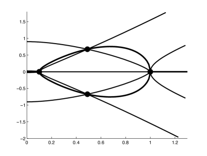
In this section, we describe the possible viscous shock profile connections for the various rest point configurations described in Section 3. Typical phase portraits (determined numerically) for the two variable system (2.22) with are graphed in Figures 7, 8, and 9.
4.1. The parallel case,
Proposition 4.1.
In the parallel case , for and , and , assuming without loss of generality that is the largest rest point of the traveling-wave equation, there is always a profile connecting and the unique parallel rest point , , , which is of Lax -type if , Lax -type if , and overcompressive type if . In the latter case, there are Lax connections from repellor to the additional saddle-type rest points
and from these saddle-type rest points to the attractor , whose orbits bound a four-sided region foliated by overcompressive connections.
Proof.
In the parallel case, (2.22) reduces to
| (4.1) | ||||
where is convex and vanishing at , , hence negative for . Setting , we find that there is a monotone decreasing solution connecting to , which has the type described by the results of Proposition 3.5.
As , the nullclines for are well-defined for , bounding a lens-shaped set between and , passing through the saddle-type rest points at and pinching to a single point at , within which . Noting that for , we find that this region is invariant in backward (resp. forward) , whence, starting at the saddles and integrating in backward (resp. forward) along the stable (resp. unstable) manifold, we find that the orbit remains for all in , hence must connect to (resp. ), verifying existence of the bounding Lax-type connections. Starting at any point lying on the open interval between the two saddles and integrating in both forward and backward , we likewise find that the orbits are all trapped in for all , so generate a one-parameter family of overcompressive connections filling up . See Figure 2. ∎
4.2. Existence of Lax-type profiles,
Proposition 4.2.
In the nonparallel case , for and , with , rest points of traveling-wave ODE (2.22) lying on the same side of always admit a Lax-type profile, which, moreover, is monotone in both and .
Proof.
Without loss of generality, let the rest points be and . Rewriting (2.22) as
| (4.2) | ||||
where is convex and (since ) negative at , hence negative on , we find that the nullclines for for are well-defined for . Likewise, the nullclines for are well-defined for on either side of , forming two disconnected branches asymptotic to the line .
Case . In this case we find that the rest points , must lie on the intersection of the lower branch of the nullcline , and the righthand () branch of the nullcline , and these nullcline branches have no other intersection (else there would be a third rest point for , impossible by Proposition 3.6). Looking at asymptotics, we find that the nullcline must lie above the nullcline for , with the two curves forming a lens-shaped region between and , within which and . Looking along the boundaries, we find that the vector field points out of , so that is invariant in backwards . Thus, integrating backward in from along the stable manifold, we find that there exists a connection to , which is monotone decreasing in and .
Case . A symmetric argument yields existence in case , again with monotone decreasing and monotone increasing, this time via invariance in forward . See Figure 3. ∎
Remark 4.3.
The argument above may be recognized as the same one used to prove existence of nonisentropic gas-dynamical profiles in [Gi]. It should be possible to obtain this result alternatively by a relative entropy argument as in [G] for the nonisentropic case, showing in case that the level set of through encloses , yielding existence by a Lyapunov-function argument in backward ; this would apply also for finite.
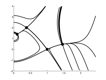
4.3. Existence of intermediate shock profiles,
Proposition 4.4.
Set . In the nonparallel case , with , for each fixed with , , and for which there exist four rest points of traveling-wave ODE (2.22), there exists a value such that: (i) for , there exist no intermediate shock profiles (i.e., the only connections are regular Lax profiles between and and and as described in Proposition 4.2); (ii) for , there exists an undercompressive profile connecting to , monotone decreasing in and increasing in , and no other intermediate shock profiles; (iii) for , there exist intermediate Lax connections from to and to , in general not monotone in or else not montone in , and a one-parameter family of overcompressive profiles from to , in general not monotone in or , with no other intermediate shock profiles.
Proof.
Referring to Figure 3(b), rewrite (2.22) again as
| (4.3) | ||||
, where (see proof of Proposition 4.2) is convex, negative on , and goes to as . Denote by and the two points at which vanishes.
The nullclines
for evidently are well-defined on , together forming a simple closed curve enclosing a region on which , as seen in Figure 3(b). Likewise, the nullclines for are well-defined for on either side of , forming two disconnected branches and asymptotic to the line , Figure 3(b).
The arc formed by the portion of from the rest point at to together with the portion of the axis from to , the portion of the axis from to the intersection of the axis with , and the portion of between the intersection of the axis with and the rest point at , the Lax connection between the rest points at and , and the portion of between the rest point at out to form a barrier to the flow in forward , through which an orbit initiating inside cannot cross, as, likewise, does the arc formed by the Lax shock between the rest points at and together with the portion of extending from the rest point at to .
Thus, the orbit initiating along the unstable manifold of the rest point at pointing in decreasing - directions, and thus initially lying inside , must either (a) strike the arc between , after which, being trapped between and , it must asymptotically approach the rest point at ; (b) strike the arc of between the rest points at and , after which, being trapped between this arc and the portion of between the rest points at and , it must asymptotically approach the rest point at ; (c) remain within the interior of and to the right of for all time, asymptotically approaching the rest point at ; or, (d) exit the interior of along the arc between the rest point at and the rest point at , after which it remains trapped outside of with increasing monotonically to .
Depending whether the orbit approaches the rest point at , approaches the rest point at , or takes , we are in cases (iii), (ii), or (i) of the proposition. But, these cases are distinguished by the location along the arc formed by the portion of the upper branch of lying below together with the portion of lying below at which the orbit exits the part of the interior of lying below , with the locations corresponding to different cases ordered in clockwise fashion along . Noting that the signs of and are constant while ; remains inside (recall that it is trapped to the right of ), and are given respectively by and times the righthand sides in (4.3), we find that the exit point moves strictly clockwise along monotonically as increases.
Thus, as asserted, there is a unique value for which exits at the rest point at , corresponding to an undercompressive connection. For , exits to the right of the rest point at , going off to infinity, and for , exits to the left of the rest point at , asymptotically approaching the rest point at , corresponding to an intermediate Lax connection and case (iii).
Note, in case (iii), that the existence of this intermediate Lax connection means that, applying a symmetric argument in backward to the orbit originating from the saddle rest point at , we find that it remains trapped within for all negative , approaching asymptotically as the rest point at The four Lax connections enclose an invariant region, within which all orbits must be overcompressive profiles connecting the rest points at and . It is clear that in general the intermediate Lax profile may leave either the interior of or the region below , hence may be nonmonotone in or but not both. Similarly, we find that the members of the family of overcompressive profiles are in general nonmonotone in or (and sometimes both).
In case (ii), or case (c) above, the profile remains for all in a region for which and , hence the profile is monotone decreasing in and increasing in . This completes the description of the phase portrait in cases (iii) and (ii), finishing the proof. ∎
Remark 4.5.
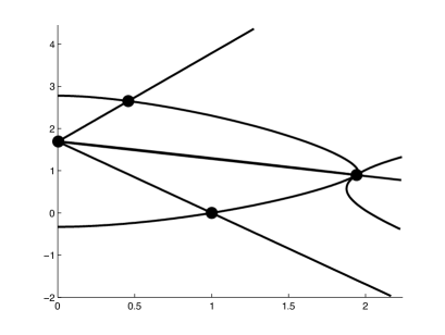
4.3.1. Singular perturbation analysis
The results of Proposition 4.4 may be illuminated somewhat by formal singular perturbation analyses as and : equivalently, taking with fixed, or with fixed. In the limit as , the phase portrait for reduces to slow flow along the nullcline (notation of the proof above), with fast flow involving jumps in the vertical direction. We find that regular Lax connections are accomplished by slow flow along , but there are no further intermediate shock connections since the branches and of are separated by the vertical line . See Figure 4(b). In the special case , the hyperbolae degenerate to the connected union of and , allowing intermediate connections both from the rest point at to the rest points at and from the rest point at to the rest point at .
In the limit as , the phase portrait reduces to slow flow along the nullcline (notation of the proof above), with fast flow involving horizontal jumps in . We find that Lax and intermediate Lax connections may all be accomplished by slow flow along , with fast flow filling in the overcompressive family. See Figure 4(a).
Finally, note that as goes from ( limit) to ( limit) the relative orientation as measured by a Melnikov separation function along an appropriate transversal of the unstable manifold pointing to the left at of the rest point associated with and the stable manifold entering from the right at of the rest point associated with changes sign. In plain language, the former passes below and to the left of the latter for and above and to the right for . By the Intermediate Value Theorem and continuous dependence, therefore, there exists at least one value for which they meet, i.e., there exists an undercompressive profile from the rest point associated with to the rest point associated with .
Remark 4.6.
The above, formal arguments, may be made rigorous as done in [FS] for the general nonisentropic case. They give slightly less information in the planar case (note that we lose the monotonicity/uniqueness of information obtained by phase plane analysis) but have the advantage of applying also to more general, nonplanar situations.
4.3.2. The undercompressive bifurcation
There is an interesting bifurcation as decreases, between the situation of case (iii) in which there is a family of overcompressive connections between the rest points at and , bounded by Lax connections, and the situation of case (i), in which there exist no intermediate shock connections. This occurs at the point where an undercompressive connection appears. As illustrated in Figures 5 and 6, this occurs through squeezing of the infinite overcompressive family to a single undercompressive–Lax profile pair, after which, as is decreased past , the undercompressive connection breaks, leaving only the regular Lax connection and no intermediate profiles remain.
4.3.3. Composite-wave limits
In the limit as , the intermediate Lax shock connecting the rest points at and approaches a “doubly composite wave” formed by an approximate superposition of the limiting undercompressive profile between the rest points at and and the Lax profile between rest points at and at value , separated by an interval of length going to infinity as on which the solution is approximately equal to the value of the saddle-type rest point at to which it passes nearby. Likewise, as , the family of intermediate overcompressive profiles connecting the rest points at and approaches a triply composite wave consisting of the approximate superposition of the limiting Lax profile between rest points at and , undercompressive profile between rest points at and , and Lax profile between rest points at and at value , separated by intervals of length going to infinity on which the solution stays near the saddle-type rest points at and .
In either case, because the resulting profiles require larger and larger intervals in to converge to limits , both the profiles and their associated Evans functions are numerically impractical to compute, requiring larger and larger computational domains, and must be handled separately taking into account the underlying limiting structure. We discuss this issue in Section 6.3
5. Evans function formulation
5.1. Two-dimensional MHD
In the two-dimensional case , (2.16) becomes
| (5.1) |
where . Linearizing about the profile solution we have
| (5.2) |
where , so that . Substituting for we obtain the eigenvalue problem
| (5.3) |
where
| (5.4) |
We let , , , and to transform to integrated coordinates. Substituting we have
| (5.5) |
Integrating from to we obtain
| (5.6) |
We use the coordinates for the Evans function formulation. Solving for the desired variables, and using , we have, finally,
| (5.7) |
This may be written as a first-order system from which the Evans function may be computed as described in Section 2.5, where
| (5.8) |
| (5.9) |
and
5.1.1. The case
In the case , with , the integrated eigenvalue equation (5.6) becomes
| (5.10) |
We use the coordinates . Solving for the desired variables, and using , , we have
| (5.11) |
This may be written as a first-order system , where
| (5.12) |
and
5.2. Three-dimensional stability
Finally, we consider the question of transverse stability, or stability with respect to three-dimensional perturbations, of a two-dimensional profile .
Carrying third components through the computations of Section 5.1, we obtain the two-dimensional integrated eigenvalue equations (5.6) augmented with the additional equations
| (5.13) |
In the case , these decouple from the rest of the equations, reducing to a transverse system
| (5.14) |
that may be studied separately. This is similar to the situation of the parallel case studied in [FT, BHZ].
5.2.1. The case
For , the transverse equations (5.14) become
| (5.15) |
This may be written as a first-order system , where
| (5.16) |
and , and used to compute a transverse Evans function determining stability with respect to perturbations in components , .
5.3. Construction of the Evans function
As described in [MaZ3, Z1], the above procedure may be carried out for general hyperbolic–parabolic systems under the standard assumptions (2.45), (2.46), (2.47), and (2.48), to express the eigenvalue problem as a first-order system with exponentially converging coefficient
| (5.17) |
where the constant is uniformly bounded on bounded domains in .
Moreover, defining we have under the same standard hypotheses the general fact [MaZ3] that, on , the system satisfies the consistent splitting hypothesis of [AGJ]: the limiting coefficient matrices have no center subspaces, and the dimensions of their stable and unstable subspaces agree and (by homotopy, using absence of center subspace) are constant throughout . Further, the associated eigenprojections, analytic on by spectral separation (again, absence of center subspace), extend analytically to , so are analytic on all of the simply connected set . By a standard construction of Kato [Kato], there exist analytically chosen bases and of the unstable subspace of and the stable subspace of , respectively.
Appealing to the general construction of Appendix D, we may thus define the Evans function as
| (5.18) |
where, for , and are analytically chosen bases of the manifolds of solutions of decaying as and , respectively, with
| (5.19) |
Evidently, (i) is analytic for , and (ii) is an eigenvalue if and only if ; see [MaZ3, Z1] for further discussion. Moreover (see Appendix D), is continuous with respect to model parameters or . The asymptotics (5.19) may be used as the basis for numerical approximation of ; see [Br1, Br2, BrZ, BDG, HuZ2, Z3, Z4].
6. Analytical stability results
We begin by recording some analytical stability analyses in special cases, in particular certain asymptotic limits (small-amplitude, composite-wave, and high-frequency limits) that are numerically difficult.
6.1. Small-amplitude stability
Consider first the small-amplitude limit, without loss of generality (after rescaling) and .
Proposition 6.1.
For , such that is a simple, genuinely nonlinear characteristic speed of the inviscid system for , there is a unique Lax-type profile connecting the rest points associated with and for sufficiently close to , and this profile is Evans, hence linearly and nonlinearly, stable (both with respect to coplanar and transverse perturbations).
6.2. Transverse stability of monotone profiles
Similarly as observed in the parallel case in [BHZ], in the case , transverse stability holds automatically for profiles that are monotone decreasing in . Thus, in our numerical stability study, it is necessary to test transverse stability only for nonmonotone profiles.
Proposition 6.2 ([BHZ]).
For , monotone-density profiles, , are Evans stable with respect to transverse perturbations: that is, they are three-dimensionally Evans stable if and only if they are two-dimensionally Evans stable.
Proof.
Dropping subscripts, we may rewrite (5.15) in symmetric form as
| (6.1) | ||||
Taking the real part of the complex -inner product of against the first equation and against the second equation and summing gives
a contradiction for and not identically zero. If on the other hand, we have a constant-coefficient equation for , which is therefore Evans stable. ∎
Remark 6.3.
In the above proof, we are using implicitly the fact that vanishing of the Evans function on , , away from essential spectrum of , implies existence of an eigenfunction decaying as [GJ1, GJ2], while vanishing at the point embedded in the essential spectrum implies existence of an eigenfunction [ZH, MaZ3].
6.3. Stability of composite waves
We consider next the numerically difficult situation as described in Section 4.3.3 of a family of profiles passing closer and closer to one or more intermediate rest points, i.e., composite wave consisting of the approximate superposition of two or more component profiles separated by a distance going to infinity. This requires a computational domain of size going to infinity, hence arbitrarily large computational effort to resolve directly. However, it may be treated in straightforward fashion by a singular perturbation analysis taking account of the limiting structure.
6.3.1. Double Lax configuration
Consider first the simplest case noted already in [Br1, Br2] of a family of overcompressive profiles in a four rest point configuration, bounded by two Lax/intermediate Lax profile pairs. Considering a family of overcompressive profiles connecting and and passing closer and closer to an intermediate saddle , parametrized by the distance of the profile from , we find that the profiles approach composite waves consisting of the approximate superposition of the bounding Lax profiles and connecting to and to , separated by a distance going to infinity as .
Proposition 6.5.
For the double-Lax configuration described, stability of and implies stability of for sufficiently small.
Proof.
By a standard multi-wave argument, as described in the conservation law setting in [Z7] and (in slightly different periodic context) [OZ], the spectrum of any such composite wave approaches the direct sum of the spectra of its component waves and as . More precisely, the Evans function associated with approaches a nonvanishing analytic multiple of the product of the Evans functions and associated with and , and so the zeros of approach the union of the zeros of and ; see [Z7] for details. In the case that and are stable Lax waves, and are nonvanishing on , and so the the union of their zeros is empty. It follows that for sufficiently small is nonvanishing on , giving the result. ∎
6.3.2. Undercompressive configurations
Next, consider the more complicated examples of Section 4.3.3, of doubly composite Lax profiles composed of the approximate superposition of a Lax profile and an undercompressive profile , and of triply composite overcompressive profiles composed of the approximate superposition of a Lax profile , an undercompressive profile , and a Lax profile , where the parameter (resp. ) indexes distance of the profile from the intermediate rest point (resp. points).
Proposition 6.6.
For either the Lax–undercompressive or Lax–undercompressive–Lax configurations described, stability of the component waves implies that has at most one unstable root.
Proof.
This follows by the observation, as in the proof of Proposition 6.5, that the zeros of approach the union of the zeros of as , together with the fact that for stable Lax waves the associated Evans function has no zeros on , while for stable undercompressive waves, the associated Evans function has a single zero at (see Proposition 2.8). From this we may conclude that has at most one zero on , giving the result. ∎
With the reduction to at most a single root, stability could in principle be decided as in [CHNZ, Z7] by examination of the mod two stability index of [GZ, MaZ3], a product of a transversality coefficient for the traveling wave connection and a low-frequency stability determinant , both real-valued, whose sign determines the parity of the number of unstable roots. The boundary case corresponds to instability through an extra root at [ZH, MaZ3]; hence, Evans stability implies nonvanishing of , , and .
The transversality coefficient is a Wronskian of the linearized traveling-wave ODE measuring transversality of the intersection of the unstable manifold at with the stable manifold at of the traveling-wave ODE, with corresponding to transversality. From the composite wave structure, we may deduce that transversality of the component waves (a consequence of Evans stability, as noted above) implies transversality of for sufficiently small, or nonvanishing of ; with further effort, the sign of may be deduced as well.
The low-frequency stability determinant is for Lax shocks equal to the Lopatinski determinant determining inviscid stability; see the discussions of [ZS, Z1]. In particular, it is independent of the nature of the viscous regularization, and readily computable. For overcompressive shocks, it involves also certain variations associated with the linearized traveling-wave ODE, as described in [ZS, Z1], which though more complicated can also be computed in the limit , deciding stability.
In the Lax–undercompressive case, we can avoid such computations by the following observation.
Corollary 6.7.
For the Lax–undercompressive configurations, suppose that the limiting endstates have a stable connecting viscous profile for some choice of viscosity ratios . Then, stability of the component waves , together with stability (resp. instability) of some composite wave for sufficiently small implies stability (resp. instability) of all composite waves for sufficiently small.
Proof.
Since the composite wave is of Lax type, is independent of the viscous regularization. It follows that for sufficiently small if there is an Evans stable profile for some choice of viscous regularization connecting the limiting endstates . (Recall from the discsussion above that Evans stability implies [MaZ3, Z1].) Since for sufficiently small, as observed previously, we thus have that for sufficiently small, and thus is of fixed sign. It follows that either all profiles are stable for sufficiently small, or no profiles are stable for sufficiently small, yielding the result. ∎
Using Corollary 6.7, we may conclude by numerical evaluations of component waves and a sample of composite waves with small but nonzero the stability of composite Lax–undercompressive waves in the numerically inaccessible limit.
Remark 6.8.
Supposing that both standard Lax and composite Lax waves composed of Lax–undercompressive waves have been determined to be stable, and viewing the Lax–undercompressive–Lax composites as the composition of LaxLax–undercompressive and Lax waves, we obtain the partial result that triply composite waves are stable for sufficiently small and , where depends on . However, to obtain a full result, it appears that one must carry out the more complicated computations described in the introductory discussion above, and so we do not complete this case.
6.4. The large-amplitude limit
We now consider behavior as shocks of different types approach their maximal amplitudes. As computed in Appendix C, for four rest point configurations, taking without loss of generality , the minimal value of is and the maximum value of is
Likewise, the minimum value of is
Thus, for fixed , , the maximum-amplitude Lax -shock connects the rest points associated with and , and the maximum-amplitude intermediate Lax -shock the rest points associated with and . The maximum-amplitude Lax -shock connects the rest points associated with and , and the maximum-amplitude intermediate Lax -shock the rest points associated with and . The maximum-amplitude (intermediate) overcompressive shock connects the rest points associated with and . For each of these limits, also .
(Here and below, we refer to two-dimensional shock types.)
Proposition 6.9.
For fixed , , the Evans function associated with Lax -shocks or intermediate Lax -shocks converges in the large-amplitude limit, uniformly on compact subsets of , to the Evans function associated with the zero-pressure limit .
Proof.
An immediate consequence of the general property of continuous dependence on parameters of the Evans function, so long as the profile remains noncharacteristic and remains bounded from the value at which the pressure function becomes singular. Noting that is bounded from the values and at which profiles become characteristic (see Appendix C.3), and that , , we obtain the result. ∎
The important implication of Proposition 6.9 is that stability of -shocks may be assessed numerically by computations on a finite mesh, even in the large-amplitude limit.
Conjecture. We conjecture that, similarly, the Evans function associated with Lax -shocks or overcompressive shocks converge in the large-amplitude limit to an Evans function associated with the zero-pressure limit .
Motivation. In the parallel case , this was shown by a delicate asymptotic ODE analysis in [HLZ, BHZ]. Our numerics (Section 7) indicate similar behavior in the general case; moreover, the limiting structure of the equations is quite similar, suggesting that the proof of [HLZ, BHZ] might extend with further care to nonzero values of .
6.4.1. Large-amplitude limit for transverse equations
As observed in [BHZ], the coefficient matrix for the transverse eigenvalue system (5.16) is smooth (indeed, linear!) in the profile variable , hence we obtain convergence in the large-amplitude limit of the transverse Evans function by the standard property of continuous dependence of the Evans function on parameters, Appendix D, so long as the profile converges uniformly exponentially to its endstates, independent of , as it does in the regular limit arising for Lax -shocks, and appears numerically to do for Lax -shocks and overcompressive shocks as well. Our numerics (Section 7) indeed suggest convergence.
6.5. The high-frequency limit
Finally, we recall the following high-frequency asymptotics established in [HLyZ1], which we will use in our numerical studies to truncate the computational domain in .
Proposition 6.10 ([HLyZ1]).
Let be the (integrated) Evans function associated with a noncharacteristic shock profile of (2.1) (with either or finite). Then, for some constants , ,
| (6.2) |
In particular, does not vanish for and sufficiently large.
Proof.
This was proved in [HLyZ1] for isentropic gas dynamics in Lagrangian coordinates by an argument using the tracking lemma of [MaZ3, PZ]. However, the same argument applies to general hyperbolic–parabolic systems satisfying the standard hypotheses (2.45), (2.46), (2.47), (2.48), with the additional property that convection in hyperbolic modes is at constant speed. In this case, hyperbolic modes are specific volume and, when , magnetic field , each of which in Lagrangian coordinates are convected with constant speed . Thus, the hypotheses are satisfied, and the result follows. (In the general case, for some , , .) ∎
7. Numerical stability investigation
In this section, we discuss our approach to Evans function computation, which is used to determine whether any unstable eigenvalues exist in our system. Our approach follows the polar-coordinate method developed in [HuZ2]; see also [BHRZ, HLZ, HLyZ1, BHZ]. Since the Evans function is analytic in the region of interest, we can numerically compute its winding number in the right-half plane around a large semicircle appropriately chosen, thus enclosing all possible unstable roots. This allows us to systematically locate roots (and hence unstable eigenvalues) within. As a result, spectral stability can be determined, and in the case of instability, one can produce bifurcation diagrams to illustrate and observe its onset. This approach was first used by Evans and Feroe [EF] and has been applied to various systems since; see for example [PSW, AS, Br2, BDG].
7.1. Approximation of the profile
Following [BHRZ, HLZ], we approximate the traveling wave profile using one of MATLAB’s boundary-value solvers bvp4c [SGT], bvp5c [KL], or bvp6c [HM], which are adaptive Lobatto quadrature schemes and can be interchanged for our purposes. These calculations are performed on a finite computational domain with projective boundary conditions . The values of approximate plus and minus spatial infinity are determined experimentally by the requirement that the absolute error be within a prescribed tolerance, say . For rigorous error/convergence bounds for these algorithms, see, e.g., [Be1, Be2].
7.2. Approximation of the Evans function
Throughout our numerical study, we use the polar-coordinate method described in [HuZ2], which encodes , where
is the exterior product encoding the minors of , “angle” is the exterior product of an orthonormal basis of evolving independently of by some implementation (e.g., Drury’s method) of continuous orthogonalization and “radius” is a complex scalar evolving by a scalar ODE slaved to , related to Abel’s formula for evolution of a full Wronskian; see [HuZ2, Z3, Z4] for further details. The Evans function is then recovered through
Here, are approximated at using asymptotics (5.19) for by
where is an analytically chosen basis for the unstable subspace of and , and then evolved using the polar coordinate ODE toward the value where the Evans function is evaluated. The requirements on approximate plus and minus spatial infinity needed for accuracy are in practice the same as the requirement already imposed in the approximation of the profile that the absolute error be within prescribed tolerance ; see [HLyZ1, Section 5.3.4] for a complete discussion. sufficed for most parameter values.
7.2.1. Shooting and initialization
The ODE calculations for individual are carried out using MATLAB’s ode45 routine, which is the adaptive 4th-order Runge-Kutta-Fehlberg method (RKF45). This method is known to have excellent accuracy with automatic error control. Typical runs involved roughly mesh points per side, with error tolerance set to AbsTol = 1e-8 and RelTol = 1e-6. To produce analytically varying Evans function output, the initializing bases are chosen analytically using Kato’s ODE; see [GZ, HuZ2, BrZ, BHZ] for further discussion. Numerical integration of Kato’s ODE is carried out using a simple second-order algorithm introduced in [Z3, Z4], a generalization of the first-order algorithm of [BrZ].
7.2.2. Winding number computation
We compute the winding number of the integrated Evans function around the around the semicircle
by varying values of along points of the contour , with mesh size taken quadratic in modulus to concentrate sample points near the origin where angles change more quickly, and summing the resulting changes in , using , available in MATLAB by direct function calls. As a check on winding number accuracy, we test a posteriori that the change in for each step is less than , and add mesh points, as necessary, to achieve this. Recall, by Rouché’s Theorem, that accuracy is preserved so long as relative variation of along each mesh interval remains less than . In Table 1 we give as a triple the radius of the domain contour, the number of mesh points, and the relative error for change in argument of between steps.
Care must be taken to choose sufficiently large to ensure any unstable eigenvalues lie inside the domain contour . Recall, Proposition 6.10, that
| (7.1) |
where and are constants. The knowledge that limit (7.1) exists allows us to determine by curve fitting of with respect to , for . When is initialized in the standard way on the real axis, so that , and are necessarily real. We then determine the necessary size of the radius by a convergence study, taking to be a value for which the relative error between and becomes less than on the entire semicircle with , indicating sufficient convergence to ensure nonvanishing. (Relative error implies nonvanishing.) For many parameter combinations, was sufficiently large, though some required a much larger radius.
Remark 7.1.
| 0.1 | (2,20,1.5(-1) | (4,20,1.8(-1) | (8,64,9.1(-2)) | (16,64,1.3(-1) | (2,20,7.6(-2)) |
|---|---|---|---|---|---|
| 0.4 | (2,20,1.1(-1)) | (2,20,3.3(-2)) | (2,20,3.1(-2)) | (2,20,3.1(-2)) | (2,20,3.2(-2)) |
| 0.6 | (2,20,7.7(-2)) | (2,20,1.6(-2)) | (2,20,1.8(-2)) | (2,20,1.7(-2)) | (2,20,1.8(-2)) |
| 0.8 | (2,20,6.6(-2)) | (2,20,2.0(-2)) | (2,20,1.9(-2)) | (2,20,1.9(-2)) | (2,20,2.0(-2)) |
7.3. Description of experiments: broad range
In our numerical study, we covered a broad intermediate parameter range to demonstrate stability of Lax and overcompressive profiles. To avoid redundancy, we discarded four rest-point configurations for which was not the largest (-value of a) rest point, since these can always be rescaled to an equivalent configuration for which is largest, hence otherwise would be counted twice. The following parameter combinations were examined, when physically meaningful, for Evans stability:
For above, the Mach number, as computed in appendix B, typically varies between and . For a little over 30 of the parameter combinations above for which , we took and attaining a Mach number of over in some cases. All Evans function computations were consistent with stability.
We also covered a broad intermediate range in terms of the parameters . When physically relevant we examined the parameter combinations:
Finally, we examined the stability of the whole family of over compressive profiles for the relevant parameters belonging to
where and is the largest value of such that the system has fixed points of the form with . For each value we examined the stability of profiles chosen by requiring they pass through evenly spaced points along the line in the phase plane connecting the two rest points with intermediate coordinates, thus insuring our profiles be representative of the family of over compressive traveling waves. In Figure 10 we plot in bold some profiles examined in our over compressive study.
In the whole investigation, each contour computed consisted of at least 40 points in . In all cases, we found the system to be Evans stable. Typical output is given in Figure 11. We remark that the Evans function is symmetric under reflections along the real axis (conjugation). Hence, we only needed to compute along half of the contour (usually 20 points in the first quadrant) to produce our results.
7.4. Composite limit
As described in Section 6.3, as overcompressive shocks approach the limit of a composite wave formed by the approximate superposition of the bounding Lax and -shocks, separated by larger and larger distance, the Evans function computation becomes prohibitively costly. However, the analytical result of Proposition 6.5 shows that we need not carry that out, since stability in the composite limit follows by stability of the component Lax waves, already tested.
7.5. Large-amplitude limit
As shown analytically in Section 6.4, the Evans functions for Lax -shocks and intermediate Lax -shocks converge in the large-amplitude limit , both for coplanar and transverse perturbations, in this case the nonphysical boundary need not be treated in any special way.
We carried out numerical case studies suggesting that the Evans function converges in the large-amplitude limit also for the more singular cases of Lax -shocks, intermediate Lax -shocks, and intermediate overcompressive shocks, left unresolved in the analytical treatment of Section 6.4. We conjecture that convergence holds also in these cases, as shown in the parallel case in [HLZ, BHZ].
A case study of the Lax -shock and intermediate Lax -shock cases is displayed in Figure 12, corresponding to a two-rest point configuration, with parameters , , , . We found stability for all amplitudes in each of these cases. We only had to take contour radius for as small as , so these runs were not computationally expensive. The Mach number for is .
A case study of the Lax -shock, intermediate Lax -shock, and intermediate overcompressive cases is displayed in Figure 13, corresponding to a four-rest point configuration, with parameters , , and , taking as small as necessary to achieve convergence: for example, in the overcompressive case, , or Mach number . In each case, convergence was achieved; likewise, we again found stability for all amplitudes. See Figure 14 for the corresponding phase portrait with , , and , approximating the limit. Note that each of the Lax -shock, intermediate Lax -shock, and intermediate overcompressive shock profiles appear to lie on a straight line orbit. It would be interesting to check whether the traveling-wave ODE, a polynomial (cubic) vector field, indeed supports exact straight line connections.
7.6. Three-dimensional stability
As discussed in section 6, transverse stability holds automatically in the case for profiles that are monotone decreasing in , so for all the studies described previously, we examined stability of (5.15) only in the case of a nonmonotone profile. All computations were consistent with stability.
7.7. The undercompressive case
For our undercompressive study we, taking care to avoid repetitions, considered the parameter combinations
for which a four rest point configuration exists in phase space. We fixed and let be a free parameter in the boundary value problem allowing us to solve simultaneously the value of for which a traveling wave connects the saddle points and for the profile itself. We successfully found and examined over 250 undercompressive profiles for Evans stability. Since undercompressive profiles are monotone implying stability in the transverse case, we only computed the Evans function associated with (5.12). Because the Evans function output for undercompressive waves has a zero at the origin, we used a small half circle of radius as part of the domain contour to skirt around the origin. All winding number results were consistent with stability. Typical output is displayed in Figure 16.
8. Discussion and open problems
In this paper, we have carried out by a combination of asymptotic ODE analysis and numerical Evans function computations a global existence/stability study for viscous shock profiles of two-dimensional isentropic magnetohydrodynamics with infinite electrical resistivity. For a monatomic -gas equation of state, and standard viscosity ration , we find that Lax and overcompressive profiles appear but undercompressive profiles do not. A systematic numerical Evans function investigation indicates that all profiles are nonlinearly stable both with respect to two-dimensional and three-dimensional perturbations. For different viscosity ratios, undercompressive shocks can appear, and these appear also to be stable with respect to two- and three-dimensional perturbations.
Our stability analysis generalizes previous viscous studies of the viscous stability problem in [FT, BHZ] for the parallel case. See also the investigations of stability in the small-magnetic field limit in [MeZ, GMWZ2]. For analyses of the related inviscid stability problem, see, e.g., [T, BT, MeZ] and references therein.
Much of the analysis carries over to the full three-dimensional case; in particular, the Rankine–Hugoniot analysis is completely general. It would be very interesting to carry out a systematic analysis in three dimensions, following the approach laid out here. Genuinely three-dimensional profiles, having a richer structure and more degrees of freedom, would appear to be a good place to look for possible instability or bifurcation. (Here, three-dimensional refers as in the present paper to the dependent variables and not the independent variable .) As noted in [TZ], instability, by stability index considerations, would for an ideal gas equation of state imply the interesting phenomenon of Hopf bifurcation to time-periodic, or “galloping” behavior at the transition to instability.
Likewise, it would be interesting to carry out the full, nonisentropic case, building on the Rankine–Hugoniot study of [FR1]. This should in principle be straightforward using the methods developed here, but more computationally intensive. We suspect that, as in the gas-dynamical case [HLyZ1], the large-amplitude limit may in fact be straightforward in this case, with bounded from the value zero at which the pressure function has a singularity. Further interesting generalizations would be to consider a Van der Waal or other “real gas” equation of state, or to include third-order dispersive effects modeling a “Hall effect” as in [DR].
Interesting boundary cases left open in the present analysis are the singular perturbation problem discussed in Section C.2 and the large-amplitude limit for Lax -shocks and overcompressives. We conjecture that in each of these cases, the Evans function converges in the limit to the Evans function for the formal pressureless gas limit . (As shown in Appendix C, all of these limits coincide with .) Our numerics are consistent with this conjecture, while the related analysis of [HLZ] gives an idea how to prove it. At the physical, modeling, level, an important problem is to determine physically interesting values of , , , and the viscosity ratio , which strongly affects solution structure as we have seen.
The absence of instabilities in our experiments suggests perhaps the more general question whether shock profiles for systems possessing a convex entropy are always stable. We do not at the moment see why this should be so, and suspect that an ideal gas equation of state is perhaps too simple an example on which to base conclusions. However, to verify or produce a counterexample to this conjecture takes on a larger importance in light of the growing body of stable examples.
Another interesting direction for further investigation would be a corresponding comprehensive study of multi-dimensional stability, as carried out for gas-dynamical shocks in [HLyZ2]. (Here, multi-dimensional refers to the independent variable .) As pointed out in [FT], instability results of [BT, T] for the corresponding inviscid problem imply that parallel shock layers become multi-dimensionally unstable for large enough magnetic field, by the general result [ZS, Z1, Z2] that inviscid stability is necessary for viscous stability, so that in multi-dimensions instability definitely occurs. The question in this case is whether viscous effects can hasten the onset of instability, that is, whether viscous instability can occur in the presence of inviscid stability.
Appendix A Signature of
Taking the Hessian of the relative entropy defined in (2.40), using (2.39), we readily obtain
| (A.1) |
yielding after a brief computation
At rest points of the traveling wave equation, we have , by (3.9), yielding , where is as defined in (3.13). This gives an explicit connection between the signature of and the sign of the derivative of the reduced Rankine–Hugoniot function .
Appendix B Computing the Mach number
The Mach number of a Lax shock is defined as
where is the downwind velocity, is the shock speed, and is the downwind sound speed (in the characteristic family of the shock), all in Eulerian coordinates. (Here, the downwind side is at , since we consider a left-moving shock.) By considering the conservation of mass equation, we have , where is density. Hence, the jump condition is given by , which implies, in the original scaling for (2.1), that
Hence,
Noting that , we simplify to get
where is the sound speed in Eulerian coordinates at , , .
Here, for Lax -shocks (resp. -shocks),
by (2.8), where denotes sound speed [A, MeZ]. In the parallel case , this gives , or , for Lax -shocks or Lax -shocks with , in agreement with the standard Mach number for gas-dynamical shocks. However, for Lax -shocks with , it gives the anomalous value . (Recall that MHD profiles in the parallel case reduce to gas-dynamical profiles.)
It is readily verified that the Mach number is invariant under the rescaling (2.15), hence gives a useful measure of shock strength in the original unrescaled coordinates. However, the example of the parallel case shows that it can give anomalous values for other than the simple gas-dynamical case. Note also that this measure of shock strength involves only the left state at , so does not distinguish between intermediate vs. regular types of shocks. We therefore use the Mach number only to give a rough idea of the strength of shocks considered in our studies, and not as a systematic measure of strength across all parameters.
Appendix C Limiting cases for Lax and overcompressive shocks
C.1.
One may ask the questions of the limits of positivity of given by (3.10). One has
| (C.1) |
The two roots of the term between brackets are real if and only if , the bracket being always positive when . In the former case, there are two roots , with for . Moreover, , so for . If , this is always true. If , it is true for , with precisely on the limiting curve above which there are no rest points with values .
Returning to the discussion, we have thus, for the two roots between and , that the limiting values of for which are , for which the factor goes to zero while the factor in brackets remains bounded, and , with the two limits coinciding precisely in the case . This means, for fixed , that in the large-amplitude limit for Lax -shocks or overcompressives (the ones involving the rest point with smallest -value, and for which ), except on the measure zero boundary . On the other hand, noting that (since the term in brackets is negative there) lies always between and , values for Lax -shocks and overcompressives remain bounded away from the value at which becomes singular, so long as .
That is, for Lax -shocks and overcompressives, the boundary of existence for fixed , is marked by the singular limit on one side, and on the other side. In the measure-zero case , the two limits agree. For Lax -shocks on the other hand, , hence only in the limit as , , and so this singular limit does not arise for , fixed. Neither does , unless .
C.2. ?
For , the upper limit for is the characteristic boundary described in Proposition 3.11. For , may take without loss of generality , where is defined as the minimum value of at which rest points appear, since in the latter case one can then rescale to the case already treated. Thus, for and bounded, may be taken always finite.
In the case , we’ve already seen in Remark 3.10 that is finite for fixed bounded from . In the case , by Remark 3.12, we have to begin with, once we eliminate four rest point configurations (as we may do by rescaling so that ). So, for fixed , we get bounded , , hence bounded by (3.10) and . Combining these observations, we find for any bounded that is also bounded from that and may be taken bounded as well. Thus, we need only consider finite parameter values for bounded and bounded from .
The sole remaining case is that of a Lax -shock, , with going to infinity and . Consulting again (C.1), we see that in this case as , so that is again uniformly bounded. (On the other hand, this case can certainly occur for sufficiently small.) The conclusion is that, without loss of generality (i.e., rescaling four rest point configurations to whenever they occur), may be taken uniformly bounded, independent of , , so that does not occur. On the other hand, the case can occur, and even , simultaneously, with remaining finite.
In this latter case, the profile ODE, and the associated stability problem, should be treatable by a singular perturbation analysis, rescaling , in which the pressure term disappears. However, we do not carry out this analysis here.
C.3. Characteristic boundaries
Other important limits are the parameter values for which the shock becomes characteristic at or , since the rate of exponential convergence of the shock profile goes to zero as they are approached, so that the length of the computational domain needed for accurate numerical approximation goes to infinity. These are given by the surfaces (corresponding to ) and (corresponding to ). The first is resolved by the analytical result of small-amplitude stability. The second requires a refined analysis outside of the scope of this paper, involving stability of characterstic shocks. For results in this direction, see [HoZ2, Ho].
Appendix D The conjugation lemma
Consider a general first-order system
| (D.1) |
with asymptotic limits as , where denote model parameters.
Lemma D.1 ([MeZ1, PZ]).
Suppose for fixed and that
| (D.2) |
for uniformly for in a neighborhood of , and that varies analytically in and smoothly (resp. continuously) in as a function into . Then, there exist in a neighborhood of invertible linear transformations and defined on and , respectively, analytic in and smooth (resp. continuous) in as functions into , such that
| (D.3) |
for any , some , and the change of coordinates reduces (D.1) to the constant-coefficient limiting systems
| (D.4) |
Proof.
The conjugators are constructed by a fixed point argument [MeZ1] as the solution of an integral equation corresponding to the homological equation
| (D.5) |
The exponential decay (D.2) is needed to make the integral equation contractive with respect to for sufficiently large. Continuity of with respect to (resp. analyticity with respect to ) then follow by continuous (resp. analytic) dependence on parameters of fixed point solutions. Here, we are using also the fact that (D.2) plus continuity of from together imply continuity of from into for any , in order to obtain the needed continuity from of the fixed point mapping. See also [PZ]. ∎
Definition D.2 (Abstract Evans function).
Suppose that on the interior of a set in , , the dimensions of the stable and unstable subspaces of remain constant, and agree at (“consistent splitting” [AGJ]), and that these subspaces have analytic bases extending continuously to boundary points of . Then, the Evans function is defined on as
| (D.6) |
where are as in Lemma D.1.
Evidently, , and , are bases for the manifolds of solutions of decaying as and , respectively, analytic in and smooth in , with as . (Here, we suppress for notational convenience.) Thus, has the alternative representation
given in (2.56).
Using the fact that as , and the fact that modes are growing as goes from to with undesired modes exponentially decaying, it is not difficult to see that the Evans function can be well-approximated by replacing with solutions of (D.1) with data
(Compare solutions and of the constant-coefficient equations .) This can be used as the basis for numerical approximation of the Evans function, as described, e.g., in [Br1, Br2, BrZ, BDG, HuZ2, Z3, Z4].
Acknowledgement. Thanks to Heinrich Freistühler and Christian Roehde for helpful orienting discussions preliminary to this project and for generously sharing information regarding their numerical existence studies in the full nonisentropic case. We gratefully acknowledge the contribution of Jeffrey Humpherys in the development of the STABLAB package with which our numerical Evans studies were carried out and in his collaboration on the series of parallel investigations [BHRZ, HLZ, CHNZ, HLyZ1, HLyZ2, BHZ], and to Tom Bridges, Gianne Derks, Jeffrey Humpherys, Bjorn Sandstede, and others, for ongoing stimulating discussions on numerical Evans function computations.
References
- [AGJ] J. Alexander, R. Gardner, and C. Jones. A topological invariant arising in the stability analysis of travelling waves. J. Reine Angew. Math., 410:167–212, 1990.
- [AMPZ] A. Azevedo, D. Marchesin, B. Plohr, and K. Zumbrun, Nonuniqueness of solutions of Riemann problems, Z. Angew. Math. Phys. 47(6):977–998, 1996.
- [AS] J. C. Alexander and R. Sachs. Linear instability of solitary waves of a Boussinesq-type equation: a computer assisted computation. Nonlinear World, 2(4):471–507, 1995.
- [A] J. E. Anderson. Magnetohydrodynamic shock waves. MIT Press, 1963.
- [BHRZ] B. Barker, J. Humpherys, K. Rudd, and K. Zumbrun. Stability of viscous shocks in isentropic gas dynamics. Comm. Math. Phys. 281, no. 1, 231–249, 2008.
- [BHZ] B. Barker, J. Humpherys, and K. Zumbrun. One-dimensional stability of parallel shock layers in isentropic magnetohydrodynamics. Preprint, 2007.
- [BeSZ] M. Beck, B. Sandstede, and K. Zumbrun, Nonlinear stability of time-periodic shock waves, to appear, Arch. Rat. Mechanics and Anal.
- [Be1] W.-J. Beyn, The numerical computation of connecting orbits in dynamical systems, IMA J. Numer. Analysis 9: 379–405, 1990.
- [Be2] W.-J. Beyn, Zur stabilit at von differenenverfahren für systeme linearer gewöhnlicher randwertaufgaben, Numer. Math. 29: 209–226, 1978.
- [C] H. Cabannes. Theoretical magnetofluiddynamics. Academic Press, New York, 1970.
- [Ba] G. K. Batchelor. An introduction to fluid dynamics. Cambridge Mathematical Library. Cambridge University Press, Cambridge, paperback edition, 1999.
- [BT] A. Blokhin and Y. Trakhinin. Stability of strong discontinuities in fluids and MHD. In Handbook of mathematical fluid dynamics, Vol. I, pages 545–652. North-Holland, Amsterdam, 2002.
- [BDG] T. J. Bridges, G. Derks, and G. Gottwald. Stability and instability of solitary waves of the fifth-order KdV equation: a numerical framework. Phys. D, 172(1-4):190–216, 2002.
- [Br1] L. Q. Brin. Numerical testing of the stability of viscous shock waves. PhD thesis, Indiana University, Bloomington, 1998.
- [Br2] L. Q. Brin. Numerical testing of the stability of viscous shock waves. Math. Comp., 70(235):1071–1088, 2001.
- [BrZ] L. Q. Brin and K. Zumbrun. Analytically varying eigenvectors and the stability of viscous shock waves. Mat. Contemp., 22:19–32, 2002. Seventh Workshop on Partial Differential Equations, Part I (Rio de Janeiro, 2001).
- [CS1] C. C. Conley and J.Smoller, On the structure of magnetohydrodynamic shock waves. Comm. Pure Appl. Math 27, 367–375, 1974.
- [CS2] C. C. Conley and J.Smoller, On the structure of magnetohydrodynamic shock waves. II. J. Math. Pures Appl. (9) no. 4, 429–443, 1975.
- [CHNZ] N. Costanzino, J. Humpherys, T. Nguyen, and K. Zumbrun. Spectral stability of noncharacteristic boundary layers of isentropic Navier–Stokes equations. Arch. Ration. Mech. Anal., to appear, 2008.
- [DR] D. Diehl and C. Rohde, On the Structure of MHD Shock Waves in Diffusive-Dispersive Media, Preprint 34, Albert-Ludwigs-Universit t Freiburg, Fakult t f r Mathematik und Physik, Mathematisches Institut, 2002.
- [EF] J. W. Evans and J. A. Feroe. Traveling waves of infinitely many pulses in nerve equations. Math. Biosci., 37:23–50, 1977.
- [FR1] H. Freistühler and C. Rohde, The bifurcation analysis of the MHD Rankine-Hugoniot equations for a perfect gas. Phys. D 185 no. 2, 78–96, 2003.
- [FR2] H. Freistühler and C. Rohde, Numerical computation of viscous profiles for hyperbolic conservation laws. Math. Comp. 71 no. 239, 1021–1042, 2002.
- [FS] H. Freistühler and P. Szmolyan, Existence and bifurcation of viscous profiles for all intermediate magnetohydrodynamic shock waves. SIAM J. Math. Anal. 26 no. 1, 112–128, 1995.
- [FT] H. Freistühler and Y. Trakhinin. On the viscous and inviscid stability of magnetohydrodynamic shock waves;. Physica D: Nonlinear Phenomena, 237(23):3030–3037, 2008.
- [FZ] H. Freistühler and K. Zumbrun, Examples of unstable viscous shock waves, unpublished research report, University of Aachen, Germany, 1998.
- [GZ] R. A. Gardner and K. Zumbrun. The gap lemma and geometric criteria for instability of viscous shock profiles. Comm. Pure Appl. Math., 51(7):797–855, 1998.
- [GJ1] R. Gardner and C.K.R.T. Jones, A stability index for steady state solutions of boundary value problems for parabolic systems, J. Diff. Eqs. 91, no. 2, 181–203, 1991.
- [GJ2] R. Gardner and C.K.R.T. Jones, Traveling waves of a perturbed diffusion equation arising in a phase field model, Ind. Univ. Math. J. 38, no. 4, 1197–1222, 1989.
- [G] P. Germain, Contribution à la théorie des ondes de choc en magnétodynamique des fluides, ONERA Publ. No. 97, Office Nat. tudes et Recherche A rospatiales, Châtillon, 1959.
- [Gi] D. Gilbarg, The existence and limit behavior of the one-dimensional shock layer. Amer. J. Math. 73:256–274, 1951.
- [GMWZ1] O. Guès, G. Métivier, M. Williams, and K. Zumbrun. Navier–Stokes regularization of multidimensional Euler shocks. Ann. Sci. École Norm. Sup. 39(4):75–175, 2006.
- [GMWZ2] O. Gues, G. Métivier, M. Williams, and K. Zumbrun. Viscous boundary value problems for symmetric systems with variable multiplicities. J. Differential Equations, 244(2):309–387, 2008.
- [He] D. Henry, Geometric theory of semilinear parabolic equations, Lecture Notes in Mathematics, Springer–Verlag, Berlin (1981), iv + 348 pp.
- [HR] P. Howard and M. Raoofi. Pointwise asymptotic behavior of perturbed viscous shock profiles. Adv. Differential Equations, 11(9):1031–1080, 2006.
- [HRZ] P. Howard, M. Raoofi, and K. Zumbrun. Sharp pointwise bounds for perturbed viscous shock waves. J. Hyperbolic Differ. Equ., 3(2):297–373, 2006.
- [HoZ1] P. Howard and K. Zumbrun. Staiblity of undercompressive shocks, J. Differential Equations 225, no. 1, 308–360, 2006.
- [HuZ1] J. Humpherys and K. Zumbrun, Spectral stability of small amplitude shock profiles for dissipative symmetric hyperbolic–parabolic systems. Z. Angew. Math. Phys. 53 (2002) 20–34.
- [HuZ2] J. Humpherys and K. Zumbrun. An efficient shooting algorithm for evans function calculations in large systems. Physica D, 220(2):116–126, 2006.
- [HLZ] J. Humpherys, O. Lafitte, and K. Zumbrun. Stability of viscous shock profiles in the high Mach number limit. Comm. Math. Phys, to appear, 2009.
- [HLyZ1] J. Humpherys, G. Lyng, and K. Zumbrun. Spectral stability of ideal-gas shock layers. Arch. Ration. Mech. Anal., to appear, 2009.
- [HLyZ2] J. Humpherys, G. Lyng, and K. Zumbrun. Multidimensional spectral stability of large-amplitude navier-stokes shocks. In preparation., 2009.
- [Ho] P. Howard. Nonlinear stability of degenerate shock profiles. Differential Integral Equations, 20(5):515–560, 2007.
- [HoZ2] P. Howard and K. Zumbrun. The Evans function and stability criteria for degenerate viscous shock waves. Discrete Contin. Dyn. Syst., 10(4):837–855, 2004.
- [HM] N. Hale and D. R. Moore. A sixth-order extension to the matlab package bvp4c of j. kierzenka and l. shampine. Technical Report NA-08/04, Oxford University Computing Laboratory, May 2008.
- [J] A. Jeffrey. Magnetohydrodynamics. University Mathematical Texts, No. 33. Oliver & Boyd, Edinburgh, 1966.
- [Kato] T. Kato. Perturbation theory for linear operators. Classics in Mathematics. Springer-Verlag, Berlin, 1995. Reprint of the 1980 edition.
- [Kaw] S. Kawashima. Systems of a hyperbolic–parabolic composite type, with applications to the equations of magnetohydrodynamics. PhD thesis, Kyoto University, 1983.
- [KL] J. Kierzenka and L. F. Shampine. A BVP solver that controls residual and error. JNAIAM J. Numer. Anal. Ind. Appl. Math., 3(1-2):27–41, 2008.
- [MeZ] G. Métivier and K. Zumbrun. Hyperbolic boundary value problems for symmetric systems with variable multiplicities. J. Differential Equations, 211(1):61–134, 2005.
- [MP] A. Majda and R. Pego, Stable viscosity matrices for systems of conservation laws, J. Diff. Eqs. 56, 229–262, 1985.
- [MaZ3] C. Mascia and K. Zumbrun. Pointwise Green function bounds for shock profiles of systems with real viscosity. Arch. Ration. Mech. Anal., 169(3):177–263, 2003.
- [MaZ4] C. Mascia and K. Zumbrun. Stability of large-amplitude viscous shock profiles of hyperbolic-parabolic systems. Arch. Ration. Mech. Anal., 172(1):93–131, 2004.
- [MeZ1] G. Métivier and K. Zumbrun, Large viscous boundary layers for noncharacteristic nonlinear hyperbolic problems, Mem. Amer. Math. Soc. 175 no. 826, vi+107 pp., 2005.
- [OZ] M. Oh and K. Zumbrun, Stability of periodic solutions of viscous conservation laws: analysis of the Evans function, Arch. Ration. Mech. Anal. 2002.
- [Pe] R. L. Pego. Stable viscosities and shock profiles for systems of conservation laws. Trans. Amer. Math. Soc., 282(2):749–763, 1984.
- [PSW] R. L. Pego, P. Smereka, and M. I. Weinstein. Oscillatory instability of traveling waves for a KdV-Burgers equation. Phys. D, 67(1-3):45–65, 1993.
- [PZ] Plaza, R. and Zumbrun, K., An Evans function approach to spectral stability of small-amplitude shock profiles, J. Disc. and Cont. Dyn. Sys., 10: 885-924, 2004.
- [Ra] M. Raoofi. asymptotic behavior of perturbed viscous shock profiles. J. Hyperbolic Differ. Equ., 2(3):595–644, 2005.
- [RZ] M. Raoofi and K. Zumbrun. Stability of undercompressive viscous shock profiles of hyperbolic-parabolic systems. J. Differential Equations, 246(4):1539–1567, 2009.
- [SGT] L. F. Shampine, I. Gladwell, and S. Thompson. Solving ODEs with MATLAB. Cambridge University Press, Cambridge, 2003.
- [TZ] B. Texier and K. Zumbrun. Hopf bifurcation of viscous shock waves in compressible gas dynamics and MHD. Arch. Ration. Mech. Anal., 190(1):107–140, 2008.
- [T] Y. Trakhinin. A complete 2D stability analysis of fast MHD shocks in an ideal gas. Comm. Math. Phys., 236(1):65–92, 2003.
- [Z1] K. Zumbrun. Stability of large-amplitude shock waves of compressible Navier-Stokes equations. In Handbook of mathematical fluid dynamics. Vol. III, pages 311–533. North-Holland, Amsterdam, 2004. With an appendix by Helge Kristian Jenssen and Gregory Lyng.
- [Z2] K. Zumbrun. Multidimensional stability of planar viscous shock waves. In Advances in the theory of shock waves, Progr. Nonlinear Differential Equations Appl., Vol. 47, pages 307–516. Birkhäuser Boston, Boston, MA, 2001.
- [Z3] K. Zumbrun. A local greedy algorithm and higher order extensions for global numerical continuation of analytically varying subspaces. to appear, Quart. Appl. Math.
- [Z4] K. Zumbrun. Numerical error analysis for evans function computations: a numerical gap lemma, centered-coordinate methods, and the unreasonable effectiveness of continuous orthogonalization, preprint, 2009.
- [Z5] K. Zumbrun. Conditional stability of unstable viscous shock waves in compressible gas dynamics and MHD, preprint, 2009.
- [Z6] K. Zumbrun. The refined inviscid stability condition and cellular instability of viscous shock waves, preprint, 2009.
- [Z7] K. Zumbrun. Stability of noncharacteristic boundary layers in the standing shock limit, to appear, Trans. AMS.
- [Z8] K. Zumbrun. Stability of viscous detonations in the ZND limit, preprint (2009).
- [ZH] K. Zumbrun and P. Howard. Pointwise semigroup methods and stability of viscous shock waves. Indiana Univ. Math. J., 47(3):741–871, 1998.
- [ZS] K. Zumbrun and D. Serre. Viscous and inviscid stability of multidimensional planar shock fronts. Indiana Univ. Math. J., 48(3):937–992, 1999.