Abstract

With a motivation to find a 2-d Lorentz-invariant solution of the $AdS_{5}\times S^{5}$ superstring we continue the study of the Pohlmeyer-reduced form of this theory. The reduced theory is constructed from currents of the superstring sigma model and is classically equivalent to it. Its action is that of $G/H=Sp(2,2)\times Sp(4)/[SU(2)]^{4}$ gauged WZW model deformed by an integrable potential and coupled to fermions. This theory is UV finite and is conjectured to be related to the superstring theory also at the quantum level. Expanded near the trivial vacuum it has the same elementary excitations (8+8 massive bosonic and fermionic 2-d degrees of freedom) as the $AdS_{5}\times S^{5}$ superstring in the $S^{5}$ light-cone gauge or near plane-wave expansion. In contrast to the superstring case, the interaction terms in the reduced action are manifestly 2-d Lorentz invariant. Since the theory is integrable, its S-matrix should be effectively determined by the two-particle scattering. Here we explicitly compute the tree-level two-particle S-matrix for the elementary excitations of the reduced theory. We find that this S-matrix has the same index structure and group factorization properties as the superstring S-matrix computed in hep-th/0611169 but has simpler coefficients, depending only on the difference of two rapidities. While the gauge-fixed form of the reduced action has only the bosonic $[SU(2)]^{4}$ part of the $PSU(2|2)\times PSU(2|2)$ symmetry of the light-cone superstring spectrum as its manifest symmetry we conjecture that it should also have a hidden fermionic symmetry that effectively interchanges bosons and fermions and which should guide us towards understanding the relation between the two S-matrices.

1 Introduction

In this paper we continue the investigation of a particular 2-d massive integrable theory which is the Pohlmeyer reduction of the $AdS_{5}\times S^{5}$ superstring theory [1, 2, 3, 4, 5]. The motivation is to use the 2-d Lorentz-invariant reduced theory as a starting point for a first-principles solution of the $AdS_{5}\times S^{5}$ superstring.

The original Pohlmeyer reduction [6] related the classical equations of motion of the $S^{2}$ sigma model to the sine-Gordon equation. In the string-theory analog of this reduction [7, 8] one considers the string on $\mathbb{R}_{t}\times S^{2}$ in the conformal gauge, fixes the residual conformal diffeomorphisms by the condition $t=\mu\tau$ and solves the Virasoro constraints in terms of one remaining degree of freedom, which is then interpreted as the sine-Gordon field. It is possible to extend this procedure to larger symmetric spaces such as $S^{n}$ and $AdS_{n}$ and then further to the full superstring theory on $AdS_{5}\times S^{5}$ (see [9, 1, 10] for details and references).

This reduction associates to a classical string theory on a coset space $F/G$ a classically equivalent “reduced” theory. In general, this reduced theory can be described as a massive deformation of a gauged $G/H$ WZW model (with an integrable potential proportional to $\mu^{2}$), which is related to a non-abelian Toda-type generalization of the sine-Gordon model. The number of independent fields in the reduced theory is the same as the number of physical degrees of freedom of the original string theory (with the conformal symmetry completely fixed and $\mu$ playing the role of a fiducial conformal scale, i.e. an analog of $p^{+}$ in a light-cone gauge). In addition, one has the advantage of manifest 2-d Lorentz symmetry in the reduced theory, which is not usually present in a light-cone gauge fixed string theory in curved target space.

This is achieved at the expense of a non-trivial transformation, essentially from coset coordinates to coset currents, that relates the fields of the original superstring theory to the fields of the reduced theory. A precise formulation of the relation between the two theories (beyond their classical equivalence including the correspondence between their integrable structures) is therefore a non-trivial open question. Since the Pohlmeyer reduction utilizes the classical conformal invariance, it has a chance to continue to apply at the quantum level only if the conformal-gauge string sigma model one starts with is UV finite. This is indeed the case for the $AdS_{5}\times S^{5}$ superstring sigma model [11] (see [12, 13] and references therein). For consistency, the corresponding reduced theory [1, 2] should also be UV finite, i.e. should have only a single “built-in” scale $\mu$. The UV finiteness of the reduced theory was shown to be the case at least to the two-loop order and is expected to be true to all loop orders [4]. Furthermore, it was conjectured in [5] that the quantum partition functions of the string theory and the reduced theory should be equal and evidence for that was provided at the leading one-loop level.

To gain better understanding of the reduced theory with the eventual goal of finding its exact solution here we will study the tree-level S-matrix for elementary excitations of this theory expanded near the trivial vacuum. The spectrum of elementary excitations contains 8 bosonic and 8 fermionic 2-d degrees of freedom of the same mass $\mu$ [1]. This is the same spectrum as found in the $S^{5}$ choice of the light-cone gauge in the $AdS_{5}\times S^{5}$ superstring theory [14, 15], but in contrast to the light-cone gauge fixed superstring action [16, 17, 18] the interaction terms in the reduced action are 2-d Lorentz invariant.

As a result, the tree-level two-particle S-matrix of the reduced theory that we will explicitly compute below is simpler than its counterpart found directly from the superstring action [19]: while the two S-matrices turn out to have the same index structure, the former depends only on the difference of the two rapidities while the latter depends on both rapidities.

The light-cone gauge $AdS_{5}\times S^{5}$ superstring S-matrix (corresponding to the spin-chain magnon S-matrix on the gauge theory side [20]) plays an important role in the conjectured Bethe Ansatz solution for the superstring energy spectrum based on its integrability and implied by the AdS/CFT correspondence, see [18] for a review and further references. Its structure is essentially fixed (up to a phase) by the residual global $PSU(2|2)\times PSU(2|2)$ symmetry of light-cone gauge Hamiltonian [21, 22, 18]. However, lack of 2-d Lorentz symmetry leads to complicated structure of the corresponding thermodynamic Bethe Ansatz for the full quantum superstring spectrum (see, e.g., [23, 24] and references therein).

The solution of the reduced theory is expected to have a simpler form. Making a natural assumption that the classical integrability of the reduced theory extends to the quantum level, its solution should be determined, as in other similar [25, 26, 27] 2-d integrable massive QFT examples [28, 29, 30, 31, 32, 33, 34, 35, 36], by an exact Lorentz-invariant S-matrix.

Let us briefly recall the structure of the reduced theory action for the $AdS_{5}\times S^{5}$ superstring (see [1, 4] for details). The starting point is the set of first-order equations of motion of the $AdS_{5}\times S^{5}$ superstring [11, 37, 38, 39] in the conformal gauge written in terms of the currents for the supercoset

$$\frac{\hat{F}}{G}=\frac{PSU(2,2|4)}{Sp(2,2)\times Sp(4)}\,.$$ (1.1)

One can solve the Virasoro conditions by choosing a particular constant matrix $T$ from the bosonic part of the coset algebra and introducing a new set of variables, i.e. fields of the reduced theory, which are algebraically related to the supercoset currents. Gauge-fixing the $\kappa$-symmetry, one can derive the remaining independent equations of motion from a local action – the reduced theory action. The latter happens to be the action of a gauged WZW model for

$$\frac{G}{H}=\frac{Sp(2,2)}{SU(2)\times SU(2)}\times\frac{Sp(4)}{SU(2)\times SU(2)}\,,$$ (1.2)

supplemented with an integrable bosonic potential and fermionic terms. The action of the gauge group $H=[SU(2)]^{4}$ commutes with the matrix $T$ so that the $T$-dependent potential is also gauge invariant. Explicitly, the reduced theory action is given by

$${S}= k \ \textrm{STr}\Big{[}\int d^{2}x\;{\textstyle{\frac{1}{2}}}\ g^{-1}\partial_{+}g\ g^{-1}\partial_{-}g\ -\,\int d^{3}x\;{\textstyle{\frac{1}{6}}}\ \epsilon^{mnl}\ g^{-1}\partial_{m}g\ g^{-1}\partial_{n}g\ g^{-1}\partial_{l}g$$ (1.3)

$$\;\;\;\;\;+\;\int d^{2}x\ \big{(}A_{+}\partial_{-}gg^{-1}-A_{-}g^{-1}\partial_{+}g-g^{-1}A_{+}gA_{-}+A_{+}A_{-}+\mu^{2}\ g^{-1}TgT\big{)}$$

$$\;\;\;\;\;+\;\int d^{2}x\ \big{(}\psi_{{}_{L}}TD_{+}\psi_{{}_{L}}+\psi_{{}_{R}}TD_{-}\psi_{{}_{R}}+\mu\;g^{-1}\psi_{{}_{L}}g\psi_{{}_{R}}\big{)}\Big{]}\,.$$

The fields in (1.3) may be represented by $8\times 8$ supermatrices in the fundamental representation of $PSU(2,2|4)$ (with diagonal $4\times 4$ blocks being bosonic and the off-diagonal $4\times 4$ blocks being fermionic). $g$ takes values in $G=Sp(2,2)\times Sp(4)$ and $A_{\pm}$ in the algebra $\mathfrak{h}$ of $H=[SU(2)]^{4}$. The fermionic fields $\psi_{{}_{L}},\psi_{{}_{R}}$ originate from particular components of the fermionic $\mathfrak{psu}(2,2|4)$ superstring currents.

In this paper we shall present the reduced-theory counterpart of the computation of the leading term in the light-cone superstring S-matrix done in [19]: we shall expand the action (1.3) around the trivial vacuum $g=\textbf{1},\,A_{\pm}=0,$ $\psi_{{}_{R}}=\psi_{{}_{L}}=0$ and find the tree-level two-particle scattering amplitude for the corresponding 8+8 massive elementary excitations. To obtain the effective quartic Lagrangian that determines this amplitude we shall choose the “light-cone” gauge $A_{+}=0$ (which preserves the Lorentz symmetry in 2-d), set $g=e^{\eta}$ and expand in powers of $\eta$. Splitting $\eta=X+\xi$, where $X$ is from the coset part of $\mathfrak{sp}(2,2)\oplus\mathfrak{sp}(4)$ and $\xi$ is from the algebra of $H$, and solving the constraint that follows from integrating out $A_{-}$ we will end up with the following equivalent Lorentz-invariant Lagrangian for the remaining 8+8 physical fields, $X$ and $\psi_{{}_{R}},\psi_{{}_{L}}$

$$\begin{split}{L}_{4}=k\;\;&\textrm{STr}\Big{(}\hskip 3.0pt\frac{1}{2}\partial_{+}X\partial_{-}X-\frac{\mu^{2}}{2}X^{2}+\psi_{{}_{L}}T\partial_{+}\psi_{{}_{L}}+\psi_{{}_{R}}T\partial_{-}\psi_{{}_{R}}+\mu\psi_{{}_{L}}\psi_{{}_{R}}\\ &\quad\hskip 5.0pt+\frac{1}{12}[X,\,\partial_{+}X][X,\,\partial_{-}X]+\frac{\mu^{2}}{24}[X,\,[X,\,T]]^{2}\\ &\quad\hskip 5.0pt-\frac{1}{4}[\psi_{{}_{L}}T,\,\psi_{{}_{L}}][X,\,\partial_{+}X]-\frac{1}{4}[\psi_{{}_{R}},\,T\psi_{{}_{R}}][X,\,\partial_{-}X]-\frac{\mu}{2}[X,\,\psi_{{}_{R}}][X,\,\psi_{{}_{L}}]\\ &\quad\hskip 5.0pt+\frac{1}{2}[\psi_{{}_{L}}T,\,\psi_{{}_{L}}][\psi_{{}_{R}},\,T\psi_{{}_{R}}]\Big{)}\,.\end{split}$$ (1.4)

The tree-level two-particle S-matrix then follows directly from the quartic terms in (1.4). The classical integrability [1] of the reduced theory (1.3) implies that the full tree-level S-matrix for the elementary excitations is determined by the two-particle S-matrix using factorization.

We shall compare the reduced-theory S-matrix following from (1.4) to the light-cone superstring one found in [19]. The two S-matrices represent the scattering of equivalent sets of degrees of freedom and turn out to have the same index structure but different kinematic coefficients. One important outstanding question is if they are actually related, e.g., by a momentum-dependent non-Lorentz invariant transformation.

To find the exact solution of the reduced theory one is to prove its quantum integrability and determine the exact quantum mass spectrum and the exact non-perturbative S-matrix. While the form of the dispersion relation in the light-cone superstring S-matrix is dictated by the centrally extended $\mathfrak{psu}(2|2)\oplus\mathfrak{psu}(2|2)$ global symmetry algebra of the light-cone Hamiltonian [21, 40, 22, 18] it remains to be understood if the exact mass spectrum of the reduced theory is also effectively controlled by symmetries, e.g., by a hidden fermionic (super)symmetry, or if one needs to resort to a study of the (semiclassical) solitonic spectrum as in [41, 42, 43].

Motivated by analogy with similar models in [27, 31, 43], the hope for solving a theory like (1.3) is based on the possibility of using methods of deformed coset CFT, i.e. on the expectation that implications of conformal symmetry should survive the $\mu$-deformation and allow one to find the exact S-matrix. Indeed, the bosonic part of the reduced theory action (1.3) is a special case of a class of massive integrable deformations of the gWZW model, generalized symmetric space sine-Gordon models or generalized non-abelian Toda-type models [44], considered in [9, 27] (see [35] for a review and references). Since the full fermionic model (1.3) is UV finite [4], we may expect some important simplifications compared to the purely bosonic cases. It is likely to be possible to prove quantum integrability by identifying (as, e.g., in [45]) a higher spin conserved current and using the bootstrap method to determine the exact S-matrix.

The structure of the rest of this paper is as follows. We shall start in section 2 with an analysis of the massive integrable deformation of the $G/H$ gauged WZW model represented by the bosonic part of (1.3). We shall choose the $A_{+}=0$ gauge, derive the bosonic part of the quartic Lagrangian (1.4) and demonstrate its classical integrability.

In section 2.4 we shall compute the corresponding two-particle S-matrix and then in section 2.5 consider two special cases $G/H\,=\,SO(N)/SO(N-1)$ and $G/H\,=\,SO(N-1,\,1)/SO(N-1)$ representing the reduced theories for strings on $\mathbb{R}_{t}\times S^{N}$ and $AdS_{N}\times S^{1}$ respectively.

In section 2.6 we shall discuss a generalization of the bosonic part of (1.3) to an asymmetrically gauged case [47, 27, 48] as the reduction procedure does not, in general, select a particular gauging of the WZW model [1]. We shall show that the corresponding tree-level S-matrix for elementary excitations does not, in fact, depend on a particular choice of the $\tau$-automorphism defining the asymmetric gauging. This will be illustrated on the example of the complex sine-Gordon model and its T-dual.

In section 3 we shall turn to the complete reduced theory (1.3) for the $AdS_{5}\times S^{5}$ superstring including the fermionic terms. Fixing the $A_{+}=0$ gauge and integrating out $A_{-}$ we will get a non-local effective Lagrangian for the physical components $X,\psi_{{}_{L}},\psi_{{}_{R}}$ but we will show that there is an equivalent local Lagrangian (1.4) that leads to the same S-matrix. In section 3.4 we shall consider the special cases of the reduced Lagrangians for the $AdS_{2}\times S^{2}$ and $AdS_{3}\times S^{3}$ superstring models and show that they agree with the corresponding special cases of (1.4).

In section 4 shall we compute the tree-level two-particle S-matrix for the complete reduced theory following from the Lagrangian (1.4). The reduced theory S-matrix turns out to be of the same group-factorizable form as in the superstring case [19], which suggests that there may be a direct relation between the two S-matrices.

In section 5 we shall make some concluding remarks and discuss open problems.

Appendix A contains some details of simplification of the gauge-fixed actions. In Appendix B we list the generators of the relevant parts of the $\mathfrak{psu}\left(2,2\,|4\right)$ algebra. In Appendix C we give explicit form of the $\mathbb{T}$-matrix of the reduced theory found in section 4. In Appendix D we consider the tree-level two-particle S-matrix of a (non-integrable) massive deformation of the bosonic geometric $G/H$ coset model and compare it to the S-matrix of the deformation of the gauged WZW model discussed in section 2.

2 Tree-level perturbative S-matrix of bosonic
gauged WZW model with an integrable potential

Before turning to the superstring case we shall start by considering a bosonic $G/H$ gauged WZW model with an integrable potential that appears [9, 1, 10] in the Pohlmeyer reduction of the geometrical $F/G$ coset sigma model, or, equivalently, is associated to a string in the conformal gauge moving on $\mathbb{R}_{t}\times F/G$ space. To carry out the reduction one writes the equations of motion for the $F/G$ model in the first-order form, i.e. in terms of currents, and then solves the Virasoro conditions by introducing a scale $\mu$, via $t=\mu\tau$, a new field $g\in G$ and a constant matrix $T$ in the coset part $\mathfrak{p}=\mathfrak{f}\ominus\mathfrak{g}$ of the algebra $\mathfrak{f}$ of $F$. $H$ is then the subgroup of $G$ whose algebra commutes with $T$ and the resulting classically equivalent integrable theory is described by a $G/H$ gWZW model with a potential determined by $T$, i.e. by the bosonic part of (1.3). The fields of the reduced theory are related to the currents of the original $F/G$ coset model [1]. Examples of such theories have been discussed, e.g., in [25, 26, 27].

The excitations around the trivial $g=\textbf{1}$ vacuum of this theory are massive (with mass $\mu$) and below we shall compute the corresponding tree-level two-particle S-matrix. Since the theory is classically integrable, this then determines the full tree-level S-matrix for elementary excitations via factorization.

2.1 Setup and notation

Since we shall view the $G/H$ gWZW model as a reduced theory for the $F/G$ coset model it is natural to think of $G$ as being embedded into a group $F$. Thus we shall consider the three groups $F\supset G\supset H$, where $F/G$ and $G/H$ are both symmetric coset spaces. The coset part of the algebra of $F$ will be denoted as $\mathfrak{p}$, i.e. $\mathfrak{f}=\mathfrak{g}\oplus\mathfrak{p}$. We shall denote the maximal abelian subalgebra of $\mathfrak{p}$ as $\mathfrak{a}$ and define $\mathfrak{n}$ as the orthogonal complement of $\mathfrak{a}$ in $\mathfrak{p}$, i.e.

$$\mathfrak{f}=\mathfrak{g}\oplus\mathfrak{p}\ ,\ \ \ \ \ \ \ \mathfrak{p}=\mathfrak{a}\oplus\mathfrak{n}\ .$$ (2.1)

We will assume that $\mathfrak{a}$ is one-dimensional and denote its non-trivial element as $T$. Then $H$ is defined as the subgroup of $G$ whose algebra $\mathfrak{h}$ is the centralizer of $T$ in $\mathfrak{g}$, i.e. $[T,\epsilon]=0,\ \epsilon\in\mathfrak{h}$. Then

$$\mathfrak{g}=\mathfrak{m}\oplus\mathfrak{h}\ ,\ \ \ \ [\mathfrak{a},\,\mathfrak{a}]=0\,,\ \ [\mathfrak{a},\,\mathfrak{h}]=0\,,\ \ \ [\mathfrak{m},\,\mathfrak{m}]\subset\mathfrak{h}\ ,\ \ \ [\mathfrak{m},\,\mathfrak{h}]\subset\mathfrak{m}\,,\ \ [\mathfrak{h},\,\mathfrak{h}]\subset\mathfrak{h}\,.$$ (2.2)

We shall also assume the following commutation relations which are all consistent with $F/G$ being a symmetric space,

$$\begin{array}[]{ccccc}[\mathfrak{a},\,\mathfrak{n}]\subset{\mathfrak{m}}\,,&[\mathfrak{a},\,\mathfrak{m}]\subset\mathfrak{n}\,,&[\mathfrak{n},\,\mathfrak{n}]\subset\mathfrak{h}\,,&[\mathfrak{n},\,\mathfrak{m}]\subset\mathfrak{a}\,,&[\mathfrak{n},\,\mathfrak{h}]\subset\mathfrak{n}\,.\end{array}$$ (2.3)

We shall consider all the fields as matrices with indices in the fundamental representation of $\mathfrak{f}$ or $F$. The corresponding orthonormal basis of generators of $\mathfrak{f}$ is ($|\mathfrak{f}|\equiv\dim\mathfrak{f}$,   $\eta_{IJ}={\rm diag}(\pm 1,...\pm 1)$)

$$[T_{I},\,T_{J}]=f_{IJ}^{\;\;\;\;K}T_{K}\ ,\ \ \ \ \ \ \ {\textrm{Tr}}(T_{I}T_{J})=\eta_{IJ}\,,\ \ \ \ \ \ I,J=0,\ldots,|\mathfrak{f}|-1\,.$$ (2.4)

We will use $\eta_{IJ}$ to raise and lower indices. Then $f_{IJK}$ is totally antisymmetric. Explicitly, the basis can be labelled as follows:

• $T_{0}=n_{0}T$:   the generator of $\mathfrak{a}$    ($|\mathfrak{a}|=1$)

• $T_{a}$: basis of $\mathfrak{m}$    ($a=1,\ldots,|\mathfrak{m}|$)

• $T_{i}$: basis of $\mathfrak{h}$   ($i=|\mathfrak{m}|+1,\ldots,|\mathfrak{g}|$)

• $T_{\hat{a}}$: basis of $\mathfrak{n}$  ($\hat{a}=|\mathfrak{g}|+1,\ldots,|\mathfrak{f}|-1$)

In this section for simplicity we will work with the assumption that $F$ is compact (and thus so are $G$ and $H$), but generalization to a non-compact case will be straightforward. Compactness implies that $\eta_{IJ}=-\delta_{IJ}$. Then ${\textrm{Tr}}(T^{2}_{0})=-1$ and thus $n_{0}$ is a normalization constant entering the expression for ${\textrm{Tr}}(T^{2})$

$${\textrm{Tr}}(T^{2})=-n_{0}^{-2}\ .$$ (2.5)

Also, for the basis of the $G/H$ part of the algebra $\mathfrak{m}$ we have

$${\textrm{Tr}}\left(T_{a}T_{b}\right)=\eta_{ab}=-\delta_{ab}\ .$$ (2.6)

We shall assume that for $m\in\mathfrak{m}$

$${\textrm{Tr}}\ ([m,\,T]^{2})={\textrm{Tr}}\left(m^{2}\right)\,,\ \ \ \ \ \ {\rm i.e.}\ \ \ n_{0}^{-2}f_{a\,0}^{\;\;\;\hat{a}}f_{b\,0\hat{a}}=-\delta_{ab}\ .$$ (2.7)

This condition implies that the spectrum of elementary excitations in the action like (1.3) will be massive with the parameter $\mu$ being the mass scale. We shall use also the following identity (below $m=m^{a}T_{a}\in\mathfrak{m}$)

$$\begin{array}[]{c}{\textrm{Tr}}([m,\,[m,\,T]]^{2})=-n_{0}^{-2}f_{a\,0}^{\;\;\;\hat{a}}f_{b\hat{a}}^{\;\;\;0}f_{c\,0}^{\;\;\;\hat{b}}f_{d\hat{b}}^{\;\;\;0}m^{a}m^{b}m^{c}m^{d}=-n_{0}^{2}\,m^{a}m_{a}m^{b}m_{b}\ .\end{array}$$ (2.8)

For a non-compact group $G$, with $H$ being its maximal compact subgroup, the sign of $\delta_{ab}$ in (2.6) and the overall sign in the action (2.9) below should be reversed. This prescription is consistent with the use of the supertrace STr in (1.3) and ensures that the propagating degrees of freedom enter the action with physical signs. In the non-compact case we will still demand (2.7), but if ${\textrm{Tr}}(T_{0}^{2})$ will change sign one will need to reverse the sign in (2.8) as well.

2.2 Expansion of action near $g=\textbf{1}$ vacuum

Our starting point is thus the (symmetrically) gauged $G/H$ WZW model with an integrable potential

$$\!\!\!\!\!\!\!\!\!\!\!\!\!\!\!\!{S}_{B}=-\,k\ {\textrm{Tr}}\Big{[}\,\int\left.d^{2}x\;\textstyle{\frac{1}{2}}\left(g^{-1}\partial_{+}g\ g^{-1}\partial_{-}g\right)\right.-\;\int d^{3}x\;\textstyle{\frac{1}{6}}\epsilon^{mnl}\left(g^{-1}\partial_{m}gg^{-1}\partial_{n}gg^{-1}\partial_{l}g\right)$$

$$\;\;\;\;\;+\,\int d^{2}x\;\left(A_{+}\partial_{-}gg^{-1}-A_{-}g^{-1}\partial_{+}g-g^{-1}A_{+}gA_{-}+A_{+}A_{-}+\mu^{2}\;\ g^{-1}TgT\right)\Big{]}\,,$$ (2.9)

where $g\in G$, $A_{\pm}\in\mathfrak{h}$ and $T$ is a constant matrix such that $[T,\,H]=0$. The action is invariant under the following gauge transformations

$$g\rightarrow h^{-1}gh\ ,\ \ \ \ \ \ \ A_{\pm}\rightarrow h^{-1}A_{\pm}h+h^{-1}\partial_{\pm}h\ ,\ \ \ \ \ \ \ \ \ h=h(x)\in H\ .$$ (2.10)

The corresponding equations of motion imply

$$\partial_{+}A_{-}-\partial_{-}A_{+}+[A_{+},\,A_{-}]=0\,,$$ (2.11)

that is the connection $A$ is flat, thus it can be gauged away on-shell. The remaining equations of motion for $g$ are then those of a non-abelian Toda model [44, 9]

$$\begin{array}[]{c}\partial_{-}(g^{-1}\partial_{+}g)=\mu^{2}[T,\,g^{-1}Tg]\,,\\ (g^{-1}\partial_{+}g)_{\mathfrak{h}}=0\ ,\ \ \ \ \ \ \ \ (\partial_{-}gg^{-1})_{\mathfrak{h}}=0\,,\end{array}$$ (2.12)

with $g=\textbf{1}$ is a trivial vacuum point.

To study the scattering of elementary excitations around this vacuum we shall set

$$g=e^{\eta}\,,\ \ \ \ \ \ \ \ \eta\in\mathfrak{g}\,,$$ (2.13)

where $\eta\rightarrow h^{-1}\eta h$ under the gauge transformations (2.10).

Expanding the action (2.9) in powers of $\eta$ we get

$$S_{B}=k\int d^{2}x\ \mathcal{L}\ ,\ \ \ \ \ \ \ \mathcal{L}=\sum_{n=1}^{\infty}\;\mathcal{L}^{(n)}\,,$$ (2.14)

$$\mathcal{L}=-{\textrm{Tr}}\bigg{(}[D_{+},\,D_{-}]\eta+\sum_{n=1}^{\infty}\frac{1}{\left(n+1\right)!}\Big{[}D_{+}\eta\,\mathfrak{L}^{n-1}_{\eta}\left(D_{-}\eta\right)-\mu^{2}\mathfrak{L}_{\eta}\left(T\right)\,\mathfrak{L}^{n-1}_{\eta}\left(\mathfrak{L}_{\eta}\left(T\right)\right)\Big{]}\bigg{)}$$

$$\;\;\;\,=-{\textrm{Tr}}\Big{[}[D_{+},\,D_{-}]\eta+D_{+}\eta\,\frac{e^{\mathfrak{L}_{\eta}}-1-\mathfrak{L}_{\eta}}{\mathfrak{L}_{\eta}^{2}}\,\left({D_{-}\eta}\right)-\mu^{2}\mathfrak{L}_{\eta}\left(T\right)\,\frac{e^{\mathfrak{L}_{\eta}}-1-\mathfrak{L}_{\eta}}{\mathfrak{L}_{\eta}^{2}}\,\left(\mathfrak{L}_{\eta}\left(T\right)\right)\Big{]},$$

or explicitly,

$$\mathcal{L}^{(1)}=-{\textrm{Tr}}\left([D_{+},\,D_{-}]\eta\right)\,,$$ (2.15)

$$\mathcal{L}^{(2)}=-{\textrm{Tr}}\Big{[}\frac{1}{2}D_{+}\eta D_{-}\eta-\frac{\mu^{2}}{2}\mathfrak{L}_{\eta}\left(T\right)\mathfrak{L}_{\eta}\left(T\right)\Big{]}\,,$$ (2.16)

$$\mathcal{L}^{(3)}=-{\textrm{Tr}}\Big{[}\frac{1}{6}D_{+}\eta\,\mathfrak{L}_{\eta}\left(D_{-}\eta\right)-\frac{\mu^{2}}{6}\mathfrak{L}_{\eta}\left(T\right)\mathfrak{L}^{2}_{\eta}\left(T\right)\Big{]}\,,$$ (2.17)

$$\mathcal{L}^{(4)}=-{\textrm{Tr}}\Big{[}\frac{1}{24}D_{+}\eta\,\mathfrak{L}^{2}_{\eta}\left(D_{-}\eta\right)-\frac{\mu^{2}}{24}\mathfrak{L}_{\eta}\left(T\right)\mathfrak{L}^{3}_{\eta}\left(T\right)\Big{]}\,,\;\ldots\,$$ (2.18)

$$D_{\pm}...\equiv\partial_{\pm}...+[A_{\pm},\,...]\,,\hskip 18.0pt\mathfrak{L}_{\eta}\left(...\right)\equiv[\eta,\,...]\,.$$ (2.19)

This expansion is manifestly gauge-invariant, e.g., invariant under the infinitesimal gauge transformations

$$\delta\eta=[\eta,\epsilon]\,,\hskip 20.0pt\delta A_{\pm}=D_{\pm}\epsilon\,,\ \ \ \ \ \ \ \epsilon(x)\in\mathfrak{h}\ .$$ (2.20)

To compute the two-particle tree-level S-matrix we will not need terms more than quartic in fields.

Next, let us decompose the fluctuation field $\eta$ into a coset (“physical”) and a subgroup (“gauge”) parts according to (2.2), i.e.

$$\eta=X+\xi\,,\hskip 5.0pt\textrm{ }\hskip 5.0pt\ \ X\in\mathfrak{m}\,,\hskip 15.0pt\xi\in\mathfrak{h}\,.$$ (2.21)

Then $\mathfrak{L}_{\eta}\left(T\right)=\mathfrak{L}_{X}\left(T\right)\equiv[X,T]$, etc. The quadratic part of the Lagrangian (2.16), which should determine the asymptotic scattering states, then takes the form

$$\mathcal{L}^{(2)}=-{\textrm{Tr}}\Big{(}\frac{1}{2}\partial_{+}X\partial_{-}X-\frac{\mu^{2}}{2}X^{2}+\frac{1}{2}\partial_{+}\xi\partial_{-}\xi+A_{+}\partial_{-}\xi-A_{-}\partial_{+}\xi\Big{)}\,.$$ (2.22)

The corresponding equations of motion (cf. (2.11),(2.12))

$$\begin{array}[]{c}\partial_{+}\partial_{-}X+\mu^{2}X=0\,,\\ \partial_{+}\partial_{-}\xi+\partial_{-}A_{+}-\partial_{+}A_{-}=0\,,\ \ \ \ \ \ \ \ \ \partial_{-}\xi=\partial_{+}\xi=0\,.\end{array}$$ (2.23)

imply that only $X$ represents propagating degrees of freedom. The apparent massless and ghost modes in the $\xi,\,A_{+},\,A_{-}$ part of (2.22) are not physical states of the theory.

2.3 $A_{+}=0$ gauge and action for physical degrees of freedom

To compute the S-matrix for physical excitations (in the $G/H$ coset directions) one needs to fix the $H$ gauge symmetry in (2.14). The final result for the S-matrix should be of course gauge-independent. One apparently obvious choice is to fix a gauge on $g$ and then integrate out $A_{\pm}$ which enter the action only algebraically. However, the resulting action for $g$ then happens to be singular when expanded near $g=\textbf{1}$ [1]. This singularity, however, is a gauge artifact (it is absent, in particular, at the level of equations of motion where one can gauge fix $A_{\pm}$ to zero).

To get a regular expansion near $g=\textbf{1}$ on should choose a gauge on $A_{\pm}$. A very natural choice is the “light-cone” gauge, $A_{+}=0$. In addition to being ghost-free (the ghost determinant is field-independent), in 2 dimensions it also preserves the Lorentz invariance of the gauge-fixed action found by setting $A_{+}=0$ in (2.15)-(2.18). The quadratic Lagrangian is given by (2.22) with $A_{+}=0$. After using integration by parts and the cyclicity of the trace the cubic and the quartic terms take the following gauge-fixed form

$$\begin{split}\mathcal{L}^{(3)}_{g.f.}&=-{\textrm{Tr}}\Big{(}\frac{1}{2}\xi[\partial_{-}X,\,\partial_{+}X]+\frac{1}{6}\partial_{+}\xi[\xi,\,\partial_{-}\xi]+\frac{1}{2}A_{-}\left([X,\,\partial_{+}X]+[\xi,\,\partial_{+}\xi]\right)\Big{)}\,,\end{split}$$ (2.24)

$$\begin{split}\mathcal{L}^{(4)}_{g.f.}&=-{\textrm{Tr}}\Big{(}-\frac{1}{24}[X,\,\partial_{+}X][X,\,\partial_{-}X]+\frac{\mu^{2}}{24}[X,\,[X,\,T]]^{2}\Big{)}\\ &\hskip 50.0pt+\mathcal{O}\left(X^{2}\xi^{2}\right)+\mathcal{O}\left(\xi^{4}\right)+\mathcal{O}\left(A_{-}X^{2}\xi\right)+\mathcal{O}\left(A_{-}\xi^{3}\right)\,.\end{split}$$ (2.25)

We will not need $\xi$-dependent terms in (2.25) to determine the tree-level two-particle S-matrix for the physical states $X$.

To explicitly decouple the unphysical degrees of freedom we may integrate out $A_{-}$ and then solve the resulting delta-function constraint expressing $\xi$ in terms of $X$. Integrating over $A_{-}$ in the sum of (2.22),(2.24) gives $(g^{-1}\partial_{+}g)_{\mathfrak{h}}=0$, i.e.

$$\partial_{+}\xi-\frac{1}{2}[X,\,\partial_{+}X]-\frac{1}{2}[\xi,\,\partial_{+}\xi]+...=0\,,$$ (2.26)

where dots stands for higher order terms. Solving for $\xi$ we find

$$\xi=\frac{1}{2}\frac{1}{\partial_{+}}[X,\,\partial_{+}X]+\mathcal{O}(X^{3})\,.$$ (2.27)

The lowest order is quadratic in $X$, which means that to find the two-particle S-matrix for $X$ we do not need to consider any higher order terms in (2.27).

The resulting effective Lagrangian for the physical degrees of freedom $X$ takes the form $\mathcal{L}_{X}=\mathcal{L}_{4X}+\mathcal{O}(X^{5})$ where

$$\begin{split}\mathcal{L}_{4X}=&-{\textrm{Tr}}\left(\frac{1}{2}\partial_{+}X\partial_{-}X-\frac{\mu^{2}}{2}X^{2}+\frac{1}{8}[X,\,\partial_{+}X]\frac{\partial_{-}}{\partial_{+}}\left([X,\,\partial_{+}X]\right)\right.\\ &\;\;\;\;\;\;\;+\frac{1}{4}[\partial_{-}X,\,\partial_{+}X]\frac{1}{\partial_{+}}[X,\,\partial_{+}X]\\ &\left.\;\;\;\;\;\;\;-\frac{1}{24}[X,\,\partial_{+}X][X,\,\partial_{-}X]+\frac{\mu^{2}}{24}[X,\,[X,\,T]]^{2}\right)\,.\end{split}$$ (2.28)

The first line in the above expression comes from (2.22), the middle line from (2.24), and the third line from (2.25). Using integration by parts (see Appendix A) eq.(2.28) can be transformed into the following local Lagrangian

$$\begin{split}\mathcal{L}_{4X}=&-{\textrm{Tr}}\Big{(}\frac{1}{2}\partial_{+}X\partial_{-}X-\frac{\mu^{2}}{2}X^{2}+\frac{1}{12}[X,\,\partial_{+}X][X,\,\partial_{-}X]+\frac{\mu^{2}}{24}[X,\,[X,\,T]]^{2}\Big{)}\,.\end{split}$$ (2.29)

In general, higher-order $X^{5}$, etc. terms in the Lagrangian (2.28) may contain non-local factors $\frac{1}{\partial_{+}}$ (familiar from light-cone gauge fixed gauge theory in 4-d) but we expect that, as happened at quartic order, they should effectively disappear (possibly after a field redefinition) and the end result should be a local Lagrangian for $X$ only.

Let us now make two remarks. First, let us comment on the residual global symmetry of the resulting Lagrangian for $X$. As follows from (2.20) and (2.2), splitting $\eta=X+\xi$ leads to the gauge transformations $\delta X=[X,\epsilon],\ \ \delta\xi=[\xi,\epsilon]$. Since the residual gauge transformations that preserve the condition $A_{+}=0$ are parametrized by $\epsilon=\epsilon(x^{-})\in\mathfrak{h}$ it then follows that the effective Lagrangian for $X$ obtained by integrating out $A_{-}$ and $\xi$ should be invariant under $\delta X=[X,\epsilon]$, i.e. should have at least global $H$ invariance

$$X\to h^{-1}Xh\ ,\ \ \ \ \ \ \ \ \ \ h={\rm const}\in H\ .$$ (2.30)

The corresponding S-matrix should then also have global $H$ symmetry.

The second comment is about integrability of the action for $X$. The theory (2.9) we started with is integrable, i.e. its equations of motion follow from a flatness condition of the Lax connection (here $z$ is a spectral parameter)

$$\omega=dx^{+}\left(g^{-1}\partial_{+}g+g^{-1}A_{+}g+z\mu T\right)+dx^{-}\left(A_{-}+z^{-1}\mu g^{-1}Tg\right)\,.$$ (2.31)

The theory for the physical excitations $X$ obtained by eliminating the gauge degrees of freedom should then also to be integrable. Indeed, one can check that the equations of motion for $X$ following from (2.29)

$$\begin{split}\partial_{+}\partial_{-}X=-\mu^{2}X&+\frac{1}{6}[\partial_{+}X,\,[X,\,\partial_{-}X]]+\frac{1}{6}[\partial_{-}X,\,[X,\,\partial_{+}X]]\\ &\hskip 50.0pt+\frac{\mu^{2}}{6}[T,\,[X,\,[X,\,[X,\,T]]]]+\mathcal{O}(X^{4})\,,\end{split}$$ (2.32)

can be obtained from the flatness condition of the following Lax connection

$$\omega_{X} = dx^{+}\Big{(}\partial_{+}X-\frac{1}{4}[X,\,\partial_{+}X]-\frac{1}{12}[X,\,[X,\,\partial_{+}X]]+z\mu T\Big{)}+dx^{-}\Big{(}\frac{1}{4}[X,\,\partial_{-}X]$$ (2.33)

$$\;\;\;+\;z^{-1}\mu\Big{[}T-[X,\,T]+\frac{1}{2}[X,\,[X,\,T]]-\frac{1}{6}[X,\,[X,\,[X,\,T]]]\Big{]}\Big{)}+\mathcal{O}(X^{4})\,.$$

The all-order completion of the Lagrangian (2.29) should again admit a Lax connection. The integrability should then imply factorization of the tree-level S-matrix for $X$, i.e. this S-matrix should be essentially determined by the two-particle scattering amplitude following from the simple quartic Lagrangian (2.29).

2.4 Tree-level two-particle S-matrix

Expanding the matrix field $X$ in the basis of generators $\{T_{a}\}$ of the coset part of the algebra of $G$ and rescaling it by the overall coefficient $k$ (the expansion parameter) in the action (2.9)

$$X=\frac{1}{\sqrt{k}}X^{a}T_{a}\,,$$ (2.34)

we can write the quartic Lagrangian corresponding to (2.29), $\mathcal{L}^{\prime}_{4X}=k\,\mathcal{L}_{4X}$, in component form

$$\mathcal{L}^{\prime}_{4X}=-\frac{1}{2}\partial_{+}X_{a}\partial_{-}X^{a}+\frac{\mu^{2}}{2}X_{a}X^{a}+\frac{1}{12k}\gamma_{abcd}X^{a}X^{c}\partial_{+}X^{b}\partial_{-}X^{d}+\frac{1}{24k}\gamma_{0}\mu^{2}X^{a}X_{a}X^{b}X_{b}\,.$$ (2.35)

Here we used the relations (2.4)–(2.8) from section 2.1 and defined the coupling constants

$$\gamma_{abcd}\equiv-f_{ab}^{\;\;\;i}f_{cdi}\ ,\ \ \ \ \ \ \ \ \gamma_{0}\equiv n_{0}^{2}\ .$$ (2.36)

Since there are no cubic terms in the Lagrangian there is only a single relevant tree-level Feynman diagram (Fig.1).

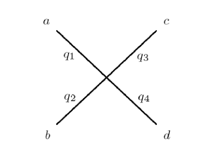
Figure 1: Scattering diagram

Using the operator approach, the usual expansion of the S-matrix may be written as

$$\mathbb{S}=1+\frac{i}{k}\mathbb{T}\,,\ \ \ \ \ \ \mathbb{T}=-k\int_{-\infty}^{\infty}d\tau\;\mathbb{V}\left(\tau\right)+\ldots\,,\ \ \ \mathbb{V}\left(\tau\right)=-\int_{-\infty}^{\infty}d\sigma\;\mathcal{L}_{int}\,,$$ (2.37)

which gives the following expression for the leading term in the $\mathbb{T}$-matrix

$$\mathbb{T}=\frac{1}{12}\int d^{2}x\Big{(}\gamma_{abcd}\,:X^{a}X^{c}\partial_{+}X^{b}\partial_{-}X^{d}:\,+\frac{1}{2}\gamma_{0}\mu^{2}\delta_{ab}\delta_{cd}\,:X^{a}X^{b}X^{c}X^{d}:\,\Big{)}\,,$$ (2.38)

where $X^{a}$ are now free-theory operators

$$X^{a}(x)=\int\frac{dp}{2\pi}\;\frac{1}{\sqrt{2\epsilon}}\left(a_{p}^{a}e^{-i\vec{p}\cdot\vec{x}}+a_{p}^{a\dagger}e^{i\vec{p}\cdot\vec{x}}\right)\Big{|}_{\epsilon\,=\,\epsilon_{p}}\,,$$ (2.39)

$$[X^{a}(\sigma),\,\dot{X}^{b}(\sigma^{\prime})]=i\delta^{ab}\delta(\sigma-\sigma^{\prime})\,,\hskip 30.0pt[a_{p}^{a},\,a_{p^{\prime}}^{b\dagger}]=(2\pi)\delta^{ab}\delta(p-p^{\prime})\,.$$ (2.40)

We use the following notation

$$\vec{x}=(\tau,\,\sigma)\ ,\ \ \ \ \ \ \vec{p}=(\epsilon,\,p)\ ,\ \ \ \ \ x^{\pm}=\frac{1}{2}(\tau\pm\sigma)\,,\hskip 30.0ptp_{\pm}=\epsilon\pm p\,,$$ (2.41)

so that $\vec{p}\,\cdot\,\vec{x}=p_{+}x^{+}+p_{-}x^{-}$. We denote the on-shell energy by $\epsilon_{p}$ and the rapidity by $\theta$:

$$\epsilon_{p}=\sqrt{p^{2}+\mu^{2}}\ ,\ \ \ \ \ \ \epsilon_{p}=\mu\cosh\theta\ ,\ \ \ \ \ \ \ p=\mu\sinh\theta\,,\ \ \ \ \ \ p_{\pm}=\mu e^{\pm\theta}\,.$$ (2.42)

We proceed by substituting $\eqref{md}$ into $\eqref{tb}$. As we are interested only in the action of $\mathbb{T}$ on two-particle states we just consider the six terms that have two creation and two annihilation operators. Integrating over $\vec{x}$ we end up with a factor $\delta^{(2)}(\vec{q}_{1}+\vec{q}_{2}-\vec{q}_{3}-\vec{q}_{4})=\delta(\epsilon_{q_{1}}+\epsilon_{q_{2}}-\epsilon_{q_{3}}-\epsilon_{q_{4}})\delta(q_{1}+q_{2}-q_{3}-q_{4})$. These two $\delta$-functions can then be used to do the integral over the momenta $q_{3}$ and $q_{4}$, as the arguments of the $\delta$-functions only vanish when either $\vec{q}_{1}=\vec{q}_{3}\hskip 5.0pt\textrm{and}\hskip 5.0pt\vec{q}_{2}=\vec{q}_{4}\,,$ or $\vec{q}_{1}=\vec{q}_{2}\hskip 5.0pt\textrm{and}\hskip 5.0pt\vec{q}_{2}=\vec{q}_{3}.$ We also pick up a Jacobian factor $\frac{\epsilon_{q_{1}}\epsilon_{q_{2}}}{|\epsilon_{q_{1}}q_{2}-q_{1}\epsilon_{q_{2}}|}\,.$ This leads to

$$\begin{split}\mathbb{T}&=\int\frac{dq_{1}dq_{2}}{(2\pi)^{2}}\frac{1}{4|\epsilon_{q_{1}}q_{2}-q_{1}\epsilon_{q_{2}}|}\Big{[}\Big{(}\frac{1}{12}\gamma_{abef}(2\mu^{2}-q_{1+}q_{2-}-q_{2+}q_{1-})\\ &\hskip 70.0pt+\frac{1}{12}\gamma_{aebf}(-4q_{1+}q_{2-})+\frac{1}{12}\gamma_{afbe}(-2\mu^{2}-q_{1+}q_{2-}-q_{2+}q_{1-})\Big{)}\\ &\hskip 70.0pt+\Big{(}\gamma_{0}\frac{\mu^{2}}{6}\delta_{ab}\delta_{ef}+\gamma_{0}\frac{\mu^{2}}{6}\delta_{ae}\delta_{bf}+\gamma_{0}\frac{\mu^{2}}{6}\delta_{af}\delta_{be}\Big{)}\Big{]}a^{a\dagger}_{q_{1}}a^{b\dagger}_{q_{2}}a^{e}_{q_{1}}a^{f}_{q_{2}}\,.\end{split}$$ (2.43)

The action of $\mathbb{T}$ on two-particle states

$$\left|X^{c}(p_{1})X^{d}(p_{2})\right>=2\sqrt{\epsilon_{p_{1}}\epsilon_{p_{2}}}a_{p_{1}}^{c\dagger}a_{p_{2}}^{d\dagger}\left|0\right>\,$$ (2.44)

gives coefficient functions $T_{ab}^{cd}(\vartheta)$

$$\mathbb{T}\left|X^{c}(p_{1})X^{d}(p_{2})\right>=T_{ab}^{cd}(\vartheta)\left|X^{a}(p_{1})X^{b}(p_{2})\right>\,.$$ (2.45)

As usual in a 2-d Lorentz invariant theory, $T_{ab}^{cd}$ should depend on the difference of the two rapidities

$$\vartheta\equiv\left|\theta_{1}-\theta_{2}\right|\,,\ \ \ \ \ \ \ \ \ \ p_{1\pm}=\mu e^{\pm\theta_{1}}\ ,\ \ \ \ p_{2\pm}=\mu e^{\pm\theta_{2}}\ .$$ (2.46)

Using that

$$a^{a\dagger}_{q_{1}}a^{b\dagger}_{q_{2}}a^{e}_{q_{1}}a^{f}_{q_{2}}\left|X^{c}(p_{1})X^{d}(p_{2})\right>$$

$$=\left(2\pi\right)^{2}\sqrt{\epsilon_{p_{1}}\epsilon_{p_{2}}}\Big{(}\delta^{ce}\delta^{df}\delta(q_{1}-p_{1})\delta(q_{2}-p_{2})+\delta^{cf}\delta^{de}\delta(q_{1}-p_{2})\delta(q_{2}-p_{1})\Big{)}a^{a\dagger}_{q_{1}}a^{b\dagger}_{q_{2}}\left|0\right>\,,$$

we end up with

$$\begin{split}T_{ab}^{cd}(\vartheta)=&\frac{1}{12\sinh\vartheta}\Big{[}\gamma_{0}\left(\delta_{ab}\delta^{cd}+\delta_{a}^{c}\delta_{b}^{d}+\delta_{a}^{d}\delta_{b}^{c}\right)+\gamma_{ab}^{\;\;\;cd}-\gamma_{a\;\,b}^{\,\;d\;\,c}\\ &.\hskip 50.0pt-\left(\gamma_{ab}^{\;\;\;cd}+2\,\gamma_{a\;\,b}^{\,\;c\;\,d}+\gamma_{a\;\,b}^{\,\;d\;\,c}\right)\cosh\vartheta\Big{]}\,.\end{split}$$ (2.47)

The same result is found by using the Feynman rules, i.e. the LSZ reduction of the four-point vertex function in (2.29). The vertex function corresponding to the diagram in Figure 1 with all the momenta $q_{i}$ flowing in is

$$\begin{split}V_{abcd}=\frac{i}{12k}\Big{(}\gamma_{abcd}\ q_{2+}q_{4-}+\frac{1}{2}\gamma_{0}{\mu^{2}}\delta_{ab}\delta_{cd}\Big{)}+\textrm{permutations}\,,\end{split}$$ (2.48)

were there are 23 permutations of $\{(a,\,q_{1}),\,(b,\,q_{2}),\,(c,\,q_{3}),\,(d,\,q_{4})\}$ other than the identity. Using that all of the legs are on-shell, i.e. $q_{1\pm}=-q_{3\pm}=\mu e^{\pm\theta_{1}}\,,\ \ q_{2\pm}=-q_{4\pm}=\mu e^{\pm\theta_{2}}\,$ we again find (2.47), with

$$T_{ab}^{cd}(\vartheta)=\frac{k}{4i\mu^{2}\sinh\vartheta}\;V_{ab}^{cd}(\vartheta)\ .$$ (2.49)

2.5 Examples: $SO(N)/SO(N-1)$ and $SO(N-1,1)/SO(N-1)$

Let us now consider two specific examples, where $G/H\,=\,SO(N)/SO(N-1)$ and $G/H\,=\,SO(N-1,\,1)/SO(N-1)$. The corresponding actions (2.9) describe Pohlmeyer reduced theories corresponding to string theory on $\mathbb{R}_{t}\times S^{N}$ and $AdS_{N}\times S^{1}$ respectively; the $N=5$ case is thus relevant for the $AdS_{5}\times S^{5}$ superstring [1]. Below we shall find the explicit expressions for the coefficients $T_{ab}^{cd}(\vartheta)$ in (2.49),(2.47).

$\mathbf{G/H\,=\,SO(N)/SO(N-1)}$

Here $F=SO(N+1),\ G=SO(N),\ H=SO(N-1)$ (cf. section 2.1). The standard normalised basis for $\mathfrak{f}=\mathfrak{so}(N+1)$ in terms of $(N+1)\times(N+1)$ matrices is

$$T_{I}=\{\tilde{T}_{\alpha\beta}\ ,\ \alpha<\beta\}\,,\hskip 20.0pt\textrm{ }\hskip 10.0pt(\tilde{T}_{\alpha\beta})_{uv}=\frac{1}{\sqrt{2}}\left(\delta_{\alpha u}\delta_{\beta v}-\delta_{\alpha v}\delta_{\beta u}\right)\,,$$ (2.50)

where $\alpha,\,\beta,\,\ldots,\,u,\,v,\ldots=1,\,\ldots,\,N+1$. As in [9, 1] we may choose $\mathfrak{g}$ to be formed by $(N+1)\times(N+1)$ matrices with non-trivial lower right $N\times N$ corner and $\mathfrak{h}$ formed by matrices with non-trivial lower right $(N-1)\times(N-1)$ corner. This corresponds to choosing the basic matrix $T$ as

$$T=\sqrt{2}\,\tilde{T}_{01}=\left(\begin{array}[]{ccccc}0&1&0&\ldots&0\\ -1&0&0&\ldots&0\\ 0&0&0&\ldots&0\\ \vdots&\vdots&\vdots&\ddots&\vdots\\ 0&0&0&\ldots&0\end{array}\right)\,.$$ (2.51)

Then $n_{0}=\frac{1}{\sqrt{2}}$ in (2.5) and the condition (2.7) is satisfied. An orthonormal basis of $\mathfrak{m}$ is given by $T_{a}=\tilde{T}_{2,a+2}$, where $a=1,\,\ldots,\,N-1$. The coupling constants defined in (2.36) are found to be

$$\gamma_{abcd}=\frac{1}{2}\left(\delta_{ac}\delta_{bd}-\delta_{ad}\delta_{bc}\right)\,,\ \ \ \ \ \ \ \ \ \gamma_{0}=\frac{1}{2}\ .$$ (2.52)

Using (2.47) we see that $T_{ab}^{cd}$ in (2.47) here simplifies to

$$\begin{split}T_{ab}^{cd}(\vartheta)=\frac{1}{8\sinh\vartheta}\Big{[}\delta_{a}^{c}\delta_{b}^{d}-\left(\delta_{ab}\delta^{cd}-\delta_{a}^{d}\delta_{b}^{c}\right)\cosh\vartheta\Big{]}\,.\end{split}$$ (2.53)

When $N=2$ the subgroup $H$ is trivial and in this case the action (2.9) reduces to that of the sine-Gordon model [9]. In this case the $G/H$ coset is one dimensional and thus (2.53) becomes

$$\begin{split}T(\vartheta)=\frac{1}{8\sinh\vartheta}\,,\end{split}$$ (2.54)

which agrees with the two-particle tree-level amplitude for scattering of elementary excitations around trivial vacuum of the sine-Gordon model.

For $N=3$ the symmetrically gauged model (2.9) is related to the complex sine-Gordon (CsG) model: fixing the $H=SO(2)$ gauge on $g$ and integrating out $A_{\pm}$ we end up with a model that is equivalent to the CsG model by 2-d duality. The above procedure based on the $A_{+}=0$ gauge leads to the S-matrix (2.53). The latter is also the same as the two-particle tree-level scattering amplitude for elementary excitations in CsG model. The reason for this relation has to do with the existence of several possible $H$ gaugings of the WZW model and will be discussed further in section 2.6.

$\mathbf{G/H\,=\,SO(N-1,1)/SO(N-1)}$

Here $F=SO(N-1,\,2),\ G=SO(N-1,\,1),\ H=SO(N-1)$. As here $G$ is non-compact and $H$ is its maximal compact subgroup, as discussed in section 2.1 the sign in the relations in (2.5),(2.6), etc. (i.e. the sign of the trace) should then be reversed. The basis for $\mathfrak{f}=\mathfrak{so}(N-1,2)$ can be chosen as

$$T_{I}=\{\tilde{T}_{\alpha\beta}\ ,\ \alpha<\beta\}\,,\hskip 20.0pt\textrm{ }\hskip 10.0pt(\tilde{T}_{\alpha\beta})^{u}_{\;v}=\frac{1}{\sqrt{2}}\left(\delta_{\alpha}^{u}\tilde{\eta}_{\beta v}-\tilde{\eta}_{\alpha v}\delta_{\beta}^{u}\right)\,,$$ (2.55)

where $\tilde{\eta}=\textrm{diag}\left(-1,-1,1,1,\ldots,1\right)$. Using the same embedding of $\mathfrak{g}$ and $\mathfrak{h}$ into $\mathfrak{f}$ as in the previous example, the choice of $T$ is then the same as in (2.51).

An orthonormal basis of the coset part of the algebra, $\mathfrak{m}$, is given by $T_{a}=\tilde{T}_{2,a+2}$, where $a=1,\,\ldots,\,N-1$. As the basis for $\mathfrak{h}$ is the same as in the previous example it is clear that changing the sign of the trace gives

$$\gamma_{abcd}=-\frac{1}{2}\left(\delta_{ac}\delta_{bd}-\delta_{ad}\delta_{bc}\right)\,,\ \ \ \ \ \ \ \ \ \gamma_{0}=-\frac{1}{2}\ ,$$ (2.56)

instead of (2.52). Using (2.47) we see that here $T_{ab}^{cd}$ simplifies to

$$\begin{split}T_{ab}^{cd}(\vartheta)=-\frac{1}{8\sinh\vartheta}\Big{[}\delta_{a}^{c}\delta_{b}^{d}-(\delta_{ab}\delta^{cd}-\delta_{a}^{d}\delta_{b}^{c})\cosh\vartheta\Big{]}\,.\end{split}$$ (2.57)

This differs from (2.53) only by the overall sign.

2.6 Asymmetrically gauged WZW model with an integrable potential

The action (2.9) we discussed above corresponds to the symmetrically gauged WZW model, but there is a more general class of models with an asymmetrical gauging of $H$. Asymmetrical gauging [47, 27, 48] uses an anomaly-free automorphism $\tau$ of the algebra $\mathfrak{h}$ (in the symmetrically gauged case $\tau={\textbf{1}}$). As discussed in [1, 3, 10, 5], an asymmetrically gauged analog of the $G/H$ gWZW action in (2.9) may also be considered as a Pohlmeyer reduction of the $F/G$ coset model.

As we shall see below, the choice of the $\tau$-automorphism does not actually affect the perturbative S-matrix of the corresponding theory, i.e. all the different anomaly-free gaugings of the WZW model with a potential have the same perturbative S-matrix. A way to see this is by observing that all dependence on $\tau$ in the action drops out in the $A_{+}=0$ gauge, so that the spectrum of excitations near the $g=\textbf{1}$ vacuum and the corresponding S-matrix do not depend on $\tau$.

The action of the asymmetrically gauged model is obtained from (2.9) by replacing the $A_{+}A_{-}$ term by $\tau(A_{+})A_{-}$, i.e. by replacing the $A_{\pm}$ dependent terms in (2.9) by

$$S_{a.g.}=-k\;\int d^{2}x\;{\textrm{Tr}}\Big{[}A_{+}\partial_{-}gg^{-1}-A_{-}g^{-1}\partial_{+}g-g^{-1}A_{+}gA_{-}+\tau(A_{+})A_{-}\Big{]}\,.$$ (2.58)

The full action is then invariant under the following gauge transformations

$$g\rightarrow h^{-1}g\hat{\tau}(h)\,,\ \ \ A_{+}\rightarrow h^{-1}A_{+}h+h^{-1}\partial_{+}h\,,\hskip 10.0ptA_{-}\rightarrow\hat{\tau}(h)^{-1}A_{-}\hat{\tau}(h)+\hat{\tau}(h)^{-1}\partial_{-}\hat{\tau}(h)\,,$$ (2.59)

where $\hat{\tau}$ is the lift of the automorphism $\tau$ from the algebra $\mathfrak{h}$ to the group $H$.

The analog of the quadratic Lagrangian before gauge-fixing (2.22) is

$$\mathcal{L}^{(2)}=-{\textrm{Tr}}\Big{[}\frac{1}{2}\partial_{+}X\partial_{-}X-\frac{\mu^{2}}{2}X^{2}+\frac{1}{2}\partial_{+}\xi\partial_{-}\xi+A_{+}\partial_{-}\xi-A_{-}\partial_{+}\xi-A_{+}A_{-}+\tau(A_{+})A_{-}\Big{]}\,,$$ (2.60)

leading to the following linearised equations of motion

$$\partial_{+}\partial_{-}X+\mu^{2}X=0\,,\ \ \ \ \ \ \ \ \partial_{+}\partial_{-}\xi+\partial_{-}A_{+}-\partial_{+}A_{-}=0\,,$$

$$\partial_{-}\xi-A_{-}+\tau^{-1}(A_{-})=0\,,\hskip 20.0pt\partial_{+}\xi+A_{+}-\tau(A_{+})=0\,.$$ (2.61)

It is easy to see that it is possible again to set $A_{\pm}=0$ by combining the equations of motion and the gauge freedom. Once $A_{\pm}=0$, it follows from (2.61) that $\xi$ is non-propagating, i.e. the physical asymptotic states are again those of the coset components $X$.

Fixing the $A_{+}=0$ (or $A_{-}=0$) gauge in the asymmetrically gauged action containing (2.58) we observe that the dependence on the choice of $\tau$-automorphism disappears so we should end up with the same (gauge-independent) S-matrix as in the symmetrically gauged case discussed above.

To give an explicit example, let us consider the case with $G/H=SO(3)/SO(2)$ embedded into $F=SO(4)$ (cf. section 2.5). Fixing the $H$-gauge on $g$ as in [1] we may parametrize it in terms of two coset coordinates $\phi,u$

$$g=e^{uT^{\prime}_{3}}e^{2\varphi T^{\prime}_{1}}e^{uT^{\prime}_{3}}\,,\ \ \ \ \ \ \ \ \ T_{I}^{\prime}=\sqrt{2}T_{I}\ ,$$ (2.62)

where $T_{1}$ is one of two coset generators and $T_{3}$ is a generator of $\mathfrak{h}=\mathfrak{so}(2)$ ($T_{I}$ are defined as in (2.50)). Starting with the symmetrically gauged action (2.9) and integrating out $A_{\pm}$ we get

$$\tilde{\mathcal{L}}_{csg}=4\big{(}\partial_{+}\varphi\partial_{-}\varphi+\cot^{2}{\varphi}\;\partial_{+}u\partial_{-}u+\frac{\mu^{2}}{2}\cos 2{\varphi}\big{)}\,.$$ (2.63)

The expansion of this Lagrangian near the trivial vacuum $g=\textbf{1}$, i.e. $\varphi=u=0$ is obviously singular. For an abelian $H$ the non-trivial choice of the $\tau$-automorphism is $\tau(\mathfrak{h})=-\mathfrak{h},\ \hat{\tau}(h)=h^{-1}$ leading to the “axially” gauged theory. Starting from (2.9) with $A_{+}A_{-}$ replaced according to (2.58) by $-A_{+}A_{-}$, choosing the condition on $g$ (now fixing the axial gauge symmetry $g\to h^{-1}gh^{-1}$) as

$$g=e^{-uT^{\prime}_{3}}e^{2\varphi T^{\prime}_{1}}e^{uT^{\prime}_{3}}\,,$$ (2.64)

and integrating out $A_{\pm}$ we then get, instead of (2.63), the complex sine-Gordon model

$$\mathcal{L}_{csg}=4\big{(}\partial_{+}\varphi\partial_{-}\varphi+\tan^{2}{\varphi}\;\partial_{+}u\partial_{-}u+\frac{\mu^{2}}{2}\cos 2\varphi\big{)}\,.$$ (2.65)

This Lagrangian has a regular expansion near $\varphi=u=0$, i.e. in the asymmetrically gauged case the choice of the gauge (2.62) is non-singular for the purpose of computing the S-matrix.

One can check directly that the resulting S-matrix for (2.65) is the same as found above in the $A_{+}=0$ gauge in the symmetrically gauged case, in agreement with the gauge-independence of the S-matrix and the above observation that the S-matrix in the $A_{+}=0$ gauge should not depend on a choice of the $\tau$-automorphism. Indeed, expanding (2.65) and introducing the two “cartesian” coordinates $z_{a}$ with the standard normalization of the kinetic term via $z_{1}+iz_{2}=2\sqrt{2}\varphi\,e^{iu}$ we get (cf. (2.35),(2.52))

$$\mathcal{L}_{csg}=\frac{1}{2}\partial_{+}z_{a}\partial_{-}z^{a}-\frac{\mu^{2}}{2}z_{a}z^{a}+\frac{1}{24}(\delta_{ac}\delta_{bd}-\delta_{ad}\delta_{bc})z^{a}z^{c}\partial_{+}z^{b}\partial_{-}z^{d}+\frac{\mu^{2}}{48}z_{a}z^{a}z_{b}z^{b}+\mathcal{O}(z^{5})\,.$$ (2.66)

This Lagrangian then leads to the same tree-level two-particle S-matrix (2.53) as the symmetrically gauged $SO(3)/SO(2)$ model.

Let us note that in the case when $H$ is abelian the sigma models obtained by integrating out $A_{\pm}$ in the symmetric and asymmetric gauged actions are related by the T-duality (or the scalar-scalar 2-d duality). This is evident, e.g., from comparing (2.63) and (2.65) (see also [49, 1]). This duality, in general, may map fluctuations near a trivial vacuum of one model into fluctuations near a non-trivial background of its dual.

The perturbative S-matrix of the complex sine-Gordon model was discussed in [50] and its exact non-perturbative (solitonic) generalisation in [41]. In particular, this theory contains non-topological solitons whose small-charge limits are the elementary excitations near the trivial vacuum we discussed above. Therefore, an appropriate limit of the full CsG S-matrix should agree with (2.53) for $N=3$. Note that this case is different from the sine-Gordon model where the solitons are topological, i.e. they interpolate between different vacua and thus do not reduce to elementary excitations in any limit.

3 Expansion of action of reduced form of
$AdS_{5}\times S^{5}$ superstring model

Let us now turn to the fermionic extension (1.3) of the gWZW model with integrable potential (2.9) arising from the Pohlmeyer reduction of the $AdS_{5}\times S^{5}$ superstring sigma model [1, 2]. The fields in this action are related to the currents of the superstring sigma model based on the supercoset $\frac{PSU(2,2|4)}{Sp(2,2)\times Sp(4)}\,.$ We shall use a particular matrix representation for these fields – the same as in [1, 4, 5]. We shall start with recalling the basic definitions and notation and then work out the expansion of the action in components, generalizing (2.35) to include the fermionic terms in (1.4).

3.1 Setup and notation

The bosonic part of the supercoset $\frac{\hat{F}}{G}=\frac{PSU(2,2|4)}{Sp(2,2)\times Sp(4)}$ is $\frac{{F}}{G}=\frac{SU(2,2)\times SU(4)}{Sp(2,2)\times Sp(4)}$. The Pohlmeyer reduction of the bosonic part produces the direct sum of the two models of the type discussed in section 2:

$$\begin{array}[]{c}F_{{}_{(1)}}=SU(2,2)\ ,\ \ \ \ \ \ \;\;\frac{G_{{}_{(1)}}}{H_{{}_{(1)}}}=\frac{Sp(2,2)}{SU(2)\times SU(2)}\,,\\ F_{{(2)}}=SU(4)\ ,\ \ \ \ \ \ \;\;\frac{G_{{}_{(2)}}}{H_{{}_{(2)}}}=\frac{Sp(4)}{SU(2)\times SU(2)}\ .\end{array}$$ (3.1)

The fields of these two models can be described together as $4\times 4$ blocks of $8\times 8$ matrices in the fundamental representation of $\hat{F}=PSU(2,2|4)$ (see [1, 4, 5] for details). Schematically, $f\in PSU(2,2|4)$ is represented by

$$\left(\begin{array}[]{cc}SU(2,2)&\ \textrm{Grassmann}\\ \ \textrm{Grassmann}&SU(4)\end{array}\right)\,.$$ (3.2)

The corresponding algebra $\hat{\mathfrak{f}}=\mathfrak{psu}\left(2,2\,|4\right)$ admits a $\mathbb{Z}_{4}$ decomposition [37]

$$\hat{\mathfrak{f}}=\mathfrak{f}_{0}\oplus\mathfrak{f}_{1}\oplus\mathfrak{f}_{2}\oplus\mathfrak{f}_{3},\,\hskip 20.0pt[\mathfrak{f}_{i},\,\mathfrak{f}_{j}]=\mathfrak{f}_{i+j\textrm{ mod }4}\,,$$ (3.3)

where $\mathfrak{f}_{0}$, $\mathfrak{f}_{2}$ are bosonic and $\mathfrak{f}_{1}$, $\mathfrak{f}_{3}$ are fermionic. These subspaces relate to those of section 2 as follows: $\mathfrak{f}_{0}=\mathfrak{g}=\mathfrak{sp}(2,2)\oplus\mathfrak{sp}(4)$ and $\mathfrak{f}_{2}=\mathfrak{p}$ is the orthogonal complement of $\mathfrak{g}$ in the bosonic part $\mathfrak{f}=\mathfrak{su}(2,2)\oplus\mathfrak{su}(4)$ of the superalgebra, i.e. $\mathfrak{p}$ is the part of the algebra that corresponds to the coset space $AdS_{5}\times S^{5}$.

The reduced action (1.3) is constructed using the supertrace

$$\textrm{STr}(f)=\sum_{i=1}^{4}f_{ii}-\sum_{i=5}^{8}f_{ii}\,,$$ (3.4)

The matrix $T$ from the maximal abelian subalgebra of $\mathfrak{p}$ satisfying the required properties is chosen as in [1]

$$T=\left(\begin{array}[]{cc}T_{{}_{(1)}}&0\\ 0&T_{{}_{(2)}}\end{array}\right)\,,\ \ \ \ T_{{(1)}}=T_{{(2)}}=\frac{i}{2}\textrm{diag}\;\left(1,\,1,\,-1,\,-1\right)\,,\hskip 20.0ptT^{2}=-\frac{1}{4}\mathbf{I}\,.$$ (3.5)

With this choice ${\textrm{Tr}}(T_{{}_{(1,2)}})^{2}=-1$, i.e. $n_{0}=1$ in (2.5). As in section 2, the subgroup $H$ of $G=Sp(2,2)\times Sp(4)$ has the algebra $\mathfrak{h}$ defined to be the centralizer of $T$. Here $H=SU(2)^{4}$, which is embedded into $8\times 8$ matrix representation of $\hat{F}=PSU(2,2|4)$ as follows

$$\left(\begin{array}[]{cccc}SU(2)_{{}_{(1)}}&0&0&0\\ 0&SU(2)_{{}_{(1^{\prime})}}&0&0\\ 0&0&SU(2)_{{}_{(2)}}&0\\ 0&0&0&SU(2)_{{}_{(2^{\prime})}}\end{array}\right)\,.$$ (3.6)

As discussed in [1], $\hat{\mathfrak{f}}$ admits also an orthogonal $\mathbb{Z}_{2}$ decomposition

$$\hat{\mathfrak{f}}=\hat{\mathfrak{f}}^{\perp}\oplus\hat{\mathfrak{f}}^{\parallel}\ ,\ \ \ \ \ \ [\hat{\mathfrak{f}}^{\perp},\,\hat{\mathfrak{f}}^{\perp}]\subset\hat{\mathfrak{f}}^{\perp}\,,\ \ \ [\hat{\mathfrak{f}}^{\parallel},\,\hat{\mathfrak{f}}^{\parallel}]\subset\hat{\mathfrak{f}}^{\perp}\,,\ \ \ [\hat{\mathfrak{f}}^{\perp},\,\hat{\mathfrak{f}}^{\parallel}]\subset\hat{\mathfrak{f}}^{\parallel}\,,$$ (3.7)

defined by $T$ as follows (${\rm f}\in\hat{\mathfrak{f}}$)

$${\rm f}={\rm f}^{\perp}+{\rm f}^{\parallel}\ ,\ \ \ \ \ \ \ [T,{\rm f}^{\perp}]=0\ ,\ \ \ \ \ \ \{T,{\rm f}^{\parallel}\}=0\ ,$$ (3.8)

i.e. $[T,\,f^{\parallel}]=2Tf^{\parallel}$,  $\textrm{STr}(f^{\perp}f^{\parallel})=0$, etc. Each of the subspaces in (3.3) then splits into $\perp$ and $\parallel$ parts and we can make the following identifications of the bosonic subspaces with the ones in (2.1),(2.2)

$$\mathfrak{f}^{\perp}_{0}=\mathfrak{h}=\mathfrak{su}(2)\oplus\mathfrak{su}(2)\oplus\mathfrak{su}(2)\oplus\mathfrak{su}(2)\ ,\ \ \ \ \ \ \mathfrak{f}^{\parallel}_{0}=\mathfrak{m}\ ,\ \ \ \ \ \ \mathfrak{f}^{\perp}_{2}=\mathfrak{a}=\{T\}\ ,\ \ \ \ \mathfrak{f}^{\parallel}_{2}=\mathfrak{n}\ .$$ (3.9)

The particular bases for $\mathfrak{f}_{0}^{\parallel},\,\mathfrak{f}_{1}^{\parallel},\,\mathfrak{f}_{3}^{\parallel}$ that we use are given in Appendix B.

3.2 Fermionic part of the action

The action for the Pohlmeyer reduction of the $AdS_{5}\times S^{5}$ superstring sigma model is given by (1.3) where

$$g\in G=Sp(2,2)\times Sp(4)\ ,\ \ \ \ \ \ A_{\pm}\in\mathfrak{f}^{\perp}_{0}=\mathfrak{su}(2)\oplus\mathfrak{su}(2)\oplus\mathfrak{su}(2)\oplus\mathfrak{su}(2)\ ,\ \ \ \ \psi_{{}_{R}}\in\mathfrak{f}_{1}^{\parallel}\,,\hskip 10.0pt\psi_{{}_{L}}\in\mathfrak{f}_{3}^{\parallel}\,\,.$$

These fields originate from particular components of the $\mathfrak{psu}\left(2,2\,|4\right)$ currents [1].

The expansion of the bosonic part of the action, i.e. (2.9), was already discussed in section 2 and here we turn to the fermionic part given by

$${S}_{F}=k\;\int d^{2}x\;\mathcal{L}_{F}\ ,\ \ \ \ \ \ \ \ \ \ \mathcal{L}_{F}=\textrm{STr}\Big{(}\psi_{{}_{L}}TD_{+}\psi_{{}_{L}}+\psi_{{}_{R}}TD_{-}\psi_{{}_{R}}+\mu g^{-1}\psi_{{}_{L}}g\psi_{{}_{R}}\Big{)}\ .$$ (3.10)

The full action (1.3) is invariant under the $H$-gauge transformations (2.10) with $\psi_{{}_{R}}$ and $\psi_{{}_{L}}$ transforming as

$$\begin{array}[]{cc}\psi_{{}_{R}}\rightarrow h^{-1}\psi_{{}_{R}}h\,,\ \ \ \ \ \ \ \ \ \ \ \ \psi_{{}_{L}}\rightarrow h^{-1}\psi_{{}_{L}}h\,.\end{array}$$ (3.11)

To expand (3.10) near $g=\textbf{1}$ we use again (2.13),(2.21), i.e.

$$g=e^{\eta},\,\hskip 20.0pt\eta=X+\xi\ \in\mathfrak{f}_{0}\,,\ \ \ \ \ \ X\in\mathfrak{f}_{0}^{\parallel}\,,\hskip 10.0pt\xi\in\mathfrak{f}_{0}^{\perp}\,.$$ (3.12)

Then (cf. (2.14))

$$\mathcal{L}_{F}=\textrm{STr}\Big{(}\psi_{{}_{L}}T\partial_{+}\psi_{{}_{L}}+\psi_{{}_{R}}T\partial_{-}\psi_{{}_{R}}+\psi_{{}_{L}}T[A_{+},\,\psi_{{}_{L}}]+\psi_{{}_{R}}T[A_{-},\,\psi_{{}_{R}}]+\mu\;\psi_{{}_{L}}e^{\mathfrak{D}_{\eta}}(\psi_{{}_{R}})\Big{)}\,.$$ (3.13)

As our aim is to compute the two-particle S-matrix for the physical fields $(X,\psi_{{}_{L}},\psi_{{}_{R}})$ we need to expand the action to quartic order in the fields only ($\mathcal{L}_{F}=\sum_{n}\mathcal{L}^{(n)}_{F}$)

$$\begin{array}[]{c}\mathcal{L}^{(2)}_{F}=\textrm{STr}\Big{(}\psi_{{}_{L}}T\partial_{+}\psi_{{}_{L}}+\psi_{{}_{R}}T\partial_{-}\psi_{{}_{R}}+\mu\;\psi_{{}_{L}}\psi_{{}_{R}}\Big{)}\,,\\ \mathcal{L}^{(3)}_{F}=\textrm{STr}\Big{(}A_{+}[\psi_{{}_{L}},\,\psi_{{}_{L}}T]+A_{-}[\psi_{{}_{R}},\,\psi_{{}_{R}}T]+\mu\;\xi[\psi_{{}_{R}},\,\psi_{{}_{L}}]\Big{)}\,,\\ \mathcal{L}^{(4)}_{F}=\textrm{STr}\Big{(}\frac{\mu}{2}\;\psi_{{}_{L}}[X,\,[X,\,\psi_{{}_{R}}]]+\frac{\mu}{2}\;\psi_{{}_{L}}[\xi,\,[\xi,\,\psi_{{}_{R}}]]\Big{)}\,.\end{array}$$ (3.14)

As follows from the quadratic Lagrangian, the fermions $\psi_{{}_{R}},\,\psi_{{}_{L}}$ have the same mass $\mu$ as the bosons $X$ (cf. (2.23)): their linearized equations of motion are

$$\partial_{+}\psi_{{}_{L}}=2\mu T\psi_{{}_{R}}\,,\hskip 20.0pt\partial_{-}\psi_{{}_{R}}=2\mu T\psi_{{}_{L}}\,,\ \ \ \ \ \ \ \ \partial_{+}\partial_{-}\psi_{{}_{L,R}}+\mu^{2}\psi_{{}_{L,R}}=0\,.$$ (3.15)

3.3 Gauge fixing and equivalent local Lagrangian

Following the discussion in section 2 we will choose the gauge $A_{+}=0$, now in the complete action (1.3) including the fermions. We can then integrate out $A_{-}$ getting a constraint on $\xi$ which generalizes (2.26)

$$-\partial_{+}\xi+\frac{1}{2}[X,\,\partial_{+}X]+[\psi_{{}_{R}},\,\psi_{{}_{R}}T]+\frac{1}{2}[\xi,\,\partial_{+}\xi]+...=0\,.$$ (3.16)

This constraint allows us to eliminate $\xi$ from the action using (cf. (2.27))

$$\xi=\frac{1}{2}\frac{1}{\partial_{+}}[X,\,\partial_{+}X]+\frac{1}{\partial_{+}}[\psi_{{}_{R}},\,\psi_{{}_{R}}T]+...\,.$$ (3.17)

Dots here stand for higher order terms we will not need. From the expansion of the bosonic (2.22),(2.24),(2.25) and the fermionic (3.14) parts of the action we then get the gauge-fixed Lagrangian for $X,\psi_{{}_{L}},\psi_{{}_{R}}$ that generalizes (2.28) and again contains no cubic interaction terms, i.e. $\mathcal{L}=\mathcal{L}_{4}+\mathcal{O}(X^{5},X^{3}\psi^{2},...)$, where

$$\begin{split}\mathcal{L}_{4}\,=&\,\textrm{STr}\Big{(}\hskip 3.0pt\frac{1}{2}\partial_{+}X\partial_{-}X-\frac{\mu^{2}}{2}X^{2}+\psi_{{}_{L}}T\partial_{+}\psi_{{}_{L}}+\psi_{{}_{R}}T\partial_{-}\psi_{{}_{R}}+\mu\psi_{{}_{L}}\psi_{{}_{R}}\\ &\,\quad\hskip 5.0pt+\frac{1}{8}[X,\,\partial_{+}X]\frac{\partial_{-}}{\partial_{+}}[X,\,\partial_{+}X]+\frac{1}{4}[\partial_{-}X,\,\partial_{+}X]\frac{1}{\partial_{+}}[X,\,\partial_{+}X]\\ &\,\quad\hskip 5.0pt-\frac{1}{24}[X,\,\partial_{+}X][X,\,\partial_{-}X]+\frac{\mu^{2}}{24}[X,\,[X,\,T]]^{2}\\ &\,\quad\hskip 5.0pt+\frac{1}{4}[X,\,\partial_{+}X]\frac{\partial_{-}}{\partial_{+}}[\psi_{{}_{R}},\,\psi_{{}_{R}}T]+\frac{1}{4}[\psi_{{}_{R}},\,\psi_{{}_{R}}T]\frac{\partial_{-}}{\partial_{+}}[X,\,\partial_{+}X]\\ &\,\quad\hskip 5.0pt+\frac{1}{2}[\partial_{-}X,\,\partial_{+}X]\frac{1}{\partial_{+}}[\psi_{{}_{R}},\,\psi_{{}_{R}}T]+\frac{\mu}{2}[\psi_{{}_{R}},\,\psi_{{}_{L}}]\frac{1}{\partial_{+}}[X,\,\partial_{+}X]-\frac{\mu}{2}[X,\,\psi_{{}_{L}}][X,\,\psi_{{}_{R}}]\\ &\,\quad\hskip 5.0pt+\frac{1}{2}[\psi_{{}_{R}},\,\psi_{{}_{R}}T]\frac{\partial_{-}}{\partial_{+}}[\psi_{{}_{R}},\,\psi_{{}_{R}}T]+\mu[\psi_{{}_{R}},\,\psi_{{}_{L}}]\frac{1}{\partial_{+}}[\psi_{{}_{R}},\,\psi_{{}_{R}}T]\Big{)}\,.\end{split}$$ (3.18)

As in (2.28) we can use integration by parts to put the bosonic part of (3.18) into the manifestly local form $\eqref{l2}$. The quartic terms containing fermions can also be simplified with the help of integration by parts and field redefinitions that amount to use of the linearized equations of motion $\partial_{+}\partial_{-}X+\mu^{2}X=0$ and (3.15) in the quartic terms in (3.18) (see Appendix A). The result is an equivalent local Lagrangian (1.4) which leads to the same two-particle S-matrix

$$\begin{split}\mathcal{L}^{\prime}_{4}\,=&\,\textrm{STr}\Big{(}\hskip 3.0pt\frac{1}{2}\partial_{+}X\partial_{-}X-\frac{\mu^{2}}{2}X^{2}+\psi_{{}_{L}}T\partial_{+}\psi_{{}_{L}}+\psi_{{}_{R}}T\partial_{-}\psi_{{}_{R}}+\mu\psi_{{}_{L}}\psi_{{}_{R}}\\ &\,\quad\hskip 5.0pt+\frac{1}{12}[X,\,\partial_{+}X][X,\,\partial_{-}X]+\frac{\mu^{2}}{24}[X,\,[X,\,T]]^{2}\\ &\,\quad\hskip 5.0pt-\frac{1}{4}[\psi_{{}_{L}}T,\,\psi_{{}_{L}}][X,\,\partial_{+}X]-\frac{1}{4}[\psi_{{}_{R}},\,T\psi_{{}_{R}}][X,\,\partial_{-}X]-\frac{\mu}{2}[X,\,\psi_{{}_{R}}][X,\,\psi_{{}_{L}}]\\ &\,\quad\hskip 5.0pt+\frac{1}{2}[\psi_{{}_{L}}T,\,\psi_{{}_{L}}][\psi_{{}_{R}},\,T\psi_{{}_{R}}]\Big{)}\,.\end{split}$$ (3.19)

We expect that this procedure can be continued to all orders in the fields, i.e. the all-order generalization of (3.18) can be transformed into a local Lagrangian for $X,\psi_{{}_{L}},\psi_{{}_{R}}$ having the same S-matrix as by the equivalence theorem [51].

Like the bosonic Lagrangian (2.29), the Lagrangian (3.18) or (3.19) is invariant under the residual global $H=SU(2)^{4}$ symmetry transformations (cf. (2.30),(3.6))

$$X\to h^{-1}Xh\ ,\ \ \ \ \ \ \psi_{{}_{L}}\to h^{-1}\psi_{{}_{L}}h\ ,\ \ \ \ \psi_{{}_{R}}\to h^{-1}\psi_{{}_{R}}h\ ,\ \ \ \ \ h={\rm const}\in H\ ,$$ (3.20)

and so that the resulting S-matrix should then have at least $SU(2)^{4}$ global symmetry.

Let us now write the Lagrangian (3.19) in component notation as in (2.35). We shall decompose $X$ and $\psi_{{}_{R}},\,\psi_{{}_{L}}$ into parts which transform in the bi-fundamental representations of pairs of the four $SU(2)$ groups that form $H$,

$$\begin{array}[]{c}X=Y+Z\,,\ \ \ \ \ \ \ \ \psi_{{}_{R}}=\zeta_{{}_{R}}+\chi_{{}_{R}}\,,\hskip 15.0pt\psi_{{}_{L}}=\zeta_{{}_{L}}+\chi_{{}_{L}}\,,\end{array}$$ (3.21)

where the fields $Y,Z,\zeta_{{}_{R}},\chi_{{}_{R}},\zeta_{{}_{L}},\chi_{{}_{L}}$ may be identified as $2\times 2$ blocks of the $8\times 8$ matrix of $\mathfrak{psu}\left(2,2\,|4\right)$, see [4] for details. Schematically, we then have for a corresponding matrix in $\mathfrak{psu}\left(2,2\,|4\right)$ (cf. (3.6))

$$\left(\begin{array}[]{cccc}\mathfrak{su}(2)_{{}_{(1)}}&Y&0&\zeta\\ Y&\mathfrak{su}(2)_{{}_{(1^{\prime})}}&\chi&0\\ 0&\chi&\mathfrak{su}(2)_{{}_{(2)}}&Z\\ \zeta&0&Z&\mathfrak{su}(2)_{{}_{(2^{\prime})}}\end{array}\right)\,.$$ (3.22)

The explicit bases of the relevant subspaces of $\mathfrak{psu}\left(2,2\,|4\right)$ are given in Appendix B. $Y$ and $Z$ each represent $4$ bosonic degrees of freedom of the reduced theory for $AdS_{5}$ and $S^{5}$ parts respectively, while the $4$ components of $\zeta_{{}_{L,R}}$ and $4$ components of $\chi_{{}_{L,R}}$ are the fermions that “intertwine” them.

One way to write the component Lagrangian in a simple form is to formally identify the actions of the pairs of $SU(2)$ subgroups of $H$ as $SU(2)_{{}_{(1)}}=SU(2)_{{}_{(2)}}$ and $SU(2)_{{}_{(1^{\prime})}}=SU(2)_{{}_{(2^{\prime})}}$ in (3.6) leaving a single “diagonal” $SU(2)\times SU(2)$ subgroup of $H$. Then (3.22) implies that all the physical fields will be in the same bi-fundamental representation of this $SU(2)\times SU(2)$ which is locally isomorphic to $SO(4)$, with the bi-fundamental representation of the former being the same as the vector representation of the latter. In this way we can rewrite the theory so that all the fields ($Y,\,Z,\,\zeta_{{}_{R}},\,\chi_{{}_{R}},\,\zeta_{{}_{L}},\,\chi_{{}_{L}}$) are labelled by indices of the same vector representation of this $SO(4)$ group.

Using the basis of the $\mathfrak{psu}\left(2,2\,|4\right)$ defined in Appendix B, we may introduce the component fields as follows

$$\begin{array}[]{cc}Y=Y^{m}T^{A}_{m}\,,&Z=Z^{m}T^{S}_{m}\,,\\ \zeta_{{}_{R}}=e^{\frac{i\pi}{4}}\zeta_{{}_{R}}^{m}T^{R_{1}}_{m}\,,&\chi_{{}_{R}}=e^{\frac{i\pi}{4}}\chi_{{}_{R}}^{m}T^{R_{2}}_{m}\,,\\ \zeta_{{}_{L}}=e^{\frac{i\pi}{4}}\zeta_{{}_{L}}^{m}T^{L_{1}}_{m}\,,&\chi_{{}_{L}}=e^{\frac{i\pi}{4}}\chi_{{}_{L}}^{m}T^{L_{2}}_{m}\,.\end{array}$$ (3.23)

We will use $m,n,...=1,2,3,4$ for $SO(4)$ vector indices which will be raised and lowered with $\delta_{mn}$. $Y^{m}$ and $Z^{m}$ are real bosonic fields and $\zeta_{{}_{R}}^{m}$, $\zeta_{{}_{L}}^{m}$, $\chi_{{}_{R}}^{m}$ and $\chi_{{}_{L}}^{m}$ are real (hermitian) Grassmann fields. Making use of the identities in Appendix B we can then rewrite (3.19) as

$$\mathcal{L}^{\prime}_{4}\, = \,\frac{1}{2}\partial_{+}Y^{m}\partial_{-}Y_{m}-\frac{\mu^{2}}{2}Y^{m}Y_{m}+\frac{1}{2}\partial_{+}Z^{m}\partial_{-}Z_{m}-\frac{\mu^{2}}{2}Z^{m}Z_{m}$$

$$+\frac{i}{2}\zeta_{{}_{L}}^{m}\partial_{+}\zeta_{{}_{L}m}+\frac{i}{2}\zeta_{{}_{R}}^{m}\partial_{-}\zeta_{{}_{R}m}+\frac{i}{2}\chi_{{}_{L}}^{m}\partial_{+}\chi_{{}_{L}m}+\frac{i}{2}\chi_{{}_{R}}^{m}\partial_{-}\chi_{{}_{R}m}-i\mu\zeta_{{}_{L}}^{m}\zeta_{{}_{R}m}-i\mu\chi_{{}_{L}}^{m}\chi_{{}_{R}m}$$

$$-\frac{1}{12}\left(Y^{m}Y^{p}\partial_{+}Y^{n}\partial_{-}Y^{q}-Z^{m}Z^{p}\partial_{+}Z^{n}\partial_{-}Z^{q}\right)\left(\delta_{mp}\delta_{nq}-\delta_{mq}\delta_{np}\right)$$

$$-\frac{\mu^{2}}{24}(Y^{m}Y_{m}Y^{n}Y_{n}-Z^{m}Z_{m}Z^{n}Z_{n})$$

$$-\frac{i}{16}C_{mnpq}\big{(}\zeta_{{}_{L}}^{m}\zeta_{{}_{L}}^{n}Y^{p}\partial_{+}Y^{q}+\zeta_{{}_{R}}^{m}\zeta_{{}_{R}}^{n}Y^{p}\partial_{-}Y^{q}+\zeta_{{}_{L}}^{m}\zeta_{{}_{L}}^{q}Z^{n}\partial_{+}Z^{p}+\zeta_{{}_{R}}^{m}\zeta_{{}_{R}}^{q}Z^{n}\partial_{-}Z^{p}$$

$$+\chi_{{}_{L}}^{m}\chi_{{}_{L}}^{q}Y^{p}\partial_{+}Y^{n}+\chi_{{}_{R}}^{m}\chi_{{}_{R}}^{q}Y^{p}\partial_{-}Y^{n}+\chi_{{}_{L}}^{m}\chi_{{}_{L}}^{n}Z^{q}\partial_{+}Z^{p}+\chi_{{}_{R}}^{m}\chi_{{}_{R}}^{n}Z^{q}\partial_{-}Z^{p}\big{)}$$

$$+\frac{i\mu}{8}(\zeta_{{}_{R}}^{m}\zeta_{{}_{L}m}+\chi_{{}_{R}}^{m}\chi_{{}_{L}m})(Y^{n}Y_{n}-Z^{n}Z_{n})+\frac{i\mu}{4}C_{mnpq}(\zeta_{{}_{R}}^{m}\chi_{{}_{L}}^{p}Y^{q}Z^{n}-\chi_{{}_{R}}^{m}\zeta_{{}_{L}}^{p}Y^{n}Z^{q})$$

$$+\frac{1}{8}\epsilon_{mnpq}(\zeta_{{}_{L}}^{m}\zeta_{{}_{L}}^{n}\zeta_{{}_{R}}^{p}\zeta_{{}_{R}}^{q}-\chi_{{}_{L}}^{m}\chi_{{}_{L}}^{n}\chi_{{}_{R}}^{p}\chi_{{}_{R}}^{q})\,,$$

where

$$C_{mnpq}\equiv-\epsilon_{mnpq}-\delta_{mp}\delta_{nq}+\delta_{mq}\delta_{np}+\delta_{mn}\delta_{pq}\,.$$ (3.25)

This component form of the Lagrangian (3.19) has the advantage of simplicity but it has only $SO(4)$ or $SU(2)\times SU(2)$ part of global symmetry $H$ as its manifest symmetry – another $SU(2)\times SU(2)$ is hidden.

It is possible to write (3.19) also in a manifestly $SU(2)^{4}$ invariant form by trading each $SO(4)$ index for a pair of $SU(2)$ ones so as to make it explicit that the fields belong to bi-fundamental representations of the four $SU(2)$ groups according to (3.22). To do so let us introduce the indices $a,\,\dot{a},\,\alpha,\dot{\alpha}$ corresponding to the fundamental representations of the four $SU(2)$’s in (3.6). Then we may re-label the fields as follows

$$\begin{array}[]{cc}Y^{m}=(\bar{\sigma}^{m})^{\dot{a}a}Y_{a\dot{a}}\,,&Y_{a\dot{a}}=(\sigma_{m})_{a\dot{a}}Y^{m}\,,\\ Z^{m}=(\bar{\sigma}^{m})^{\dot{\alpha}\alpha}Z_{\alpha\dot{\alpha}}\,,&Z_{\alpha\dot{\alpha}}=(\sigma_{m})_{\alpha\dot{\alpha}}Z^{m}\,,\\ \zeta^{m}=(\bar{\sigma}^{m})^{\dot{\alpha}a}\zeta_{a\dot{\alpha}}\,,&\zeta_{a\dot{\alpha}}=(\sigma_{m})_{a\dot{\alpha}}\zeta^{m}\,,\\ \chi^{m}=(\bar{\sigma}^{m})^{\dot{a}\alpha}\chi_{\alpha\dot{a}}\,,&\chi_{\alpha\dot{a}}=(\sigma_{m})_{\alpha\dot{a}}\chi^{m}\end{array}$$ (3.26)

where $(Y_{a\dot{a}})^{*}=Y^{\dot{a}a}$, etc. The explicit result of the translation of (3.3) into this manifestly $SU(2)^{4}$ invariant form is

$$\mathcal{L}^{\prime}_{4}\;= \frac{1}{2}\partial_{+}Y_{a\dot{a}}\partial_{-}Y^{\dot{a}a}-\frac{\mu^{2}}{2}Y_{a\dot{a}}Y^{\dot{a}a}+\frac{1}{2}\partial_{+}Z_{\alpha\dot{\alpha}}\partial_{-}Z^{\dot{\alpha}\alpha}-\frac{\mu^{2}}{2}Z_{\alpha\dot{\alpha}}Z^{\dot{\alpha}\alpha}$$ (3.28)

$$+\frac{i}{2}{\zeta_{{}_{L}}}_{a\dot{\alpha}}\partial_{+}\zeta_{{}_{L}}^{\dot{\alpha}a}+\frac{i}{2}{\zeta_{{}_{R}}}_{a\dot{\alpha}}\partial_{-}\zeta_{{}_{R}}^{\dot{\alpha}a}+\frac{i}{2}{\chi_{{}_{L}}}_{\alpha\dot{a}}\partial_{+}\chi_{{}_{L}}^{\dot{a}\alpha}+\frac{i}{2}{\chi_{{}_{R}}}_{\alpha\dot{a}}\partial_{-}\chi_{{}_{R}}^{\dot{a}\alpha}-i\mu{\zeta_{{}_{L}}}_{a\dot{\alpha}}\zeta_{{}_{R}}^{\dot{\alpha}a}-i\mu{\chi_{{}_{L}}}_{\alpha\dot{a}}\chi_{{}_{R}}^{\dot{a}\alpha}$$

$$-\frac{1}{12}\big{(}Y_{a\dot{a}}Y^{\dot{a}a}\partial_{+}Y_{b\dot{b}}\partial_{-}Y^{\dot{b}b}-Y_{a\dot{a}}\partial_{+}Y^{\dot{a}a}Y_{b\dot{b}}\partial_{-}Y^{\dot{b}b}+\frac{\mu^{2}}{2}Y_{a\dot{a}}Y^{\dot{a}a}Y_{b\dot{b}}Y^{\dot{b}b}\big{)}$$

$$+\frac{1}{12}\big{(}Z_{\alpha\dot{\alpha}}Z^{\dot{\alpha}\alpha}\partial_{+}Z_{\beta\dot{\beta}}\partial_{-}Z^{\dot{\beta}\beta}-Z_{\alpha\dot{\alpha}}\partial_{+}Z^{\dot{\alpha}\alpha}Z_{\beta\dot{\beta}}\partial_{-}Z^{\dot{\beta}\beta}+\frac{\mu^{2}}{2}Z_{\alpha\dot{\alpha}}Z^{\dot{\alpha}\alpha}Z_{\beta\dot{\beta}}Z^{\dot{\beta}\beta}\big{)}$$

$$+\frac{i}{8}\big{(}{\zeta_{{}_{L}}}_{a\dot{\alpha}}{\zeta_{{}_{L}}}^{\dot{\alpha}b}Y^{\dot{b}a}\partial_{+}Y_{b\dot{b}}+{\zeta_{{}_{R}}}_{a\dot{\alpha}}{\zeta_{{}_{R}}}^{\dot{\alpha}b}Y^{\dot{b}a}\partial_{-}Y_{b\dot{b}}+\mu\,{\zeta_{{}_{R}}}_{a\dot{\alpha}}\zeta_{{}_{L}}^{\dot{\alpha}a}Y_{b\dot{b}}Y^{\dot{b}b}\big{)}$$

$$-\frac{i}{8}\big{(}{\zeta_{{}_{L}}}_{a\dot{\alpha}}{\zeta_{{}_{L}}}^{\dot{\beta}a}Z^{\dot{\alpha}\beta}\partial_{+}Z_{\beta\dot{\beta}}+{\zeta_{{}_{R}}}_{a\dot{\alpha}}{\zeta_{{}_{R}}}^{\dot{\beta}a}Z^{\dot{\alpha}\beta}\partial_{-}Z_{\beta\dot{\beta}}+\mu\,{\zeta_{{}_{R}}}_{a\dot{\alpha}}\zeta_{{}_{L}}^{\dot{\alpha}a}Z_{\beta\dot{\beta}}Z^{\dot{\beta}\beta}\big{)}$$

$$+\frac{i}{8}\big{(}{\chi_{{}_{L}}}_{\alpha\dot{a}}{\chi_{{}_{L}}}^{\dot{b}\alpha}Y^{\dot{a}b}\partial_{+}Y_{b\dot{b}}+{\chi_{{}_{R}}}_{\alpha\dot{a}}{\chi_{{}_{R}}}^{\dot{b}\alpha}Y^{\dot{a}b}\partial_{-}Y_{b\dot{b}}+\mu\,{\chi_{{}_{R}}}_{\alpha\dot{a}}\chi_{{}_{L}}^{\dot{a}\alpha}Y_{b\dot{b}}Y^{\dot{b}b}\big{)}$$

$$-\frac{i}{8}\big{(}{\chi_{{}_{L}}}_{\alpha\dot{a}}{\chi_{{}_{L}}}^{\dot{a}\beta}Z^{\dot{\beta}\alpha}\partial_{+}Z_{\beta\dot{\beta}}+{\chi_{{}_{R}}}_{\alpha\dot{a}}{\chi_{{}_{R}}}^{\dot{a}\beta}Z^{\dot{\beta}\alpha}\partial_{-}Z_{\beta\dot{\beta}}+\mu\,{\chi_{{}_{R}}}_{\alpha\dot{a}}\chi_{{}_{L}}^{\dot{a}\alpha}Z_{\beta\dot{\beta}}Z^{\dot{\beta}\beta}\big{)}$$

$$+\frac{i\mu}{2}\big{(}{\zeta_{{}_{R}}}_{a\dot{\alpha}}{\chi_{{}_{L}}}_{\beta\dot{b}}Y^{\dot{b}a}Z^{\dot{\alpha}\beta}-{\chi_{{}_{R}}}_{\alpha\dot{a}}{\zeta_{{}_{L}}}_{b\dot{\beta}}Y^{\dot{a}b}Z^{\dot{\beta}\alpha}\big{)}+\frac{1}{2}\big{(}{\zeta_{{}_{L}}}_{a\dot{\alpha}}{\zeta_{{}_{L}}}_{b\dot{\beta}}\zeta_{{}_{R}}^{\dot{\alpha}b}\zeta_{{}_{R}}^{\dot{\beta}a}-{\chi_{{}_{L}}}_{\alpha\dot{a}}{\chi_{{}_{L}}}_{\beta\dot{b}}\chi_{{}_{R}}^{\dot{a}\beta}\chi_{{}_{R}}^{\dot{b}\alpha}\big{)}\,.$$

The Lagrangian (3.3) or (3.28) is also manifestly 2-d Lorentz invariant, assuming that the fermions transform as Majorana-Weyl 2-d spinors [1].

The original reduced model [4] was shown to be UV finite to the two-loop order (and conjectured to be finite to all orders) in [4]; the same should of course be true also for its gauge-fixed version (3.19) or (3.3). This implies that the corresponding quantum S-matrix should be finite, i.e. should depend only on the original tree-level mass scale $\mu$.

3.4 Special cases: reduced Lagrangians for $AdS_{2}\times S^{2}$ and $AdS_{3}\times S^{3}$

Let us now look at some special cases of (3.3) corresponding to the reductions of the superstring theory on $AdS_{2}\times S^{2}$ [1] and on $AdS_{3}\times S^{3}$ [3].

Replacing $PSU(2,2|4)$ with $PSU(1,1|2)$ gives superstring theory on $AdS_{2}\times S^{2}$ and the corresponding reduced theory can be identified [1] with the (2,2) supersymmetric sine-Gordon model [46]. Its Lagrangian may be written as [1]

$$\mathcal{L} = 2\Big{[}\partial_{+}\phi\partial_{-}\phi+\partial_{+}\varphi\partial_{-}\varphi+\frac{\mu^{2}}{2}\left(\cos 2\varphi-\cosh 2\phi\right)+i\,\alpha\partial_{-}\alpha+i\,\delta\partial_{-}\delta+i\,\nu\partial_{+}\nu+i\,\rho\partial_{+}\rho$$ (3.29)

$$\hskip 15.0pt-2i\mu\Big{(}\cosh\phi\cos\varphi\ \left(\nu\delta+\rho\alpha\right)+\sinh\phi\sin\varphi\ (-\rho\delta+\nu\alpha)\Big{)}\Big{]}\,.$$

Here $\phi,\,\varphi$ are real bosonic fields and $\alpha,\,\delta,\,\nu,\,\rho$ are real (hermitian) fermions. Expanding this Lagrangian to quartic order, rescaling the fields by $\frac{1}{2}$ and renaming them, one finds that it becomes the same as (3.3) if all $SO(4)$ indices there take just only one value, i.e.

$$\begin{split}\mathcal{L}_{4}=&\frac{1}{2}\partial_{+}Y\partial_{-}Y-\frac{\mu^{2}}{2}Y^{2}+\frac{1}{2}\partial_{+}Z\partial_{-}Z-\frac{\mu^{2}}{2}Z^{2}\\ &+\frac{i}{2}\zeta_{{}_{L}}\partial_{+}\zeta_{{}_{L}}+\frac{i}{2}\zeta_{{}_{R}}\partial_{-}\zeta_{{}_{R}}+\frac{i}{2}\chi_{{}_{L}}\partial_{+}\chi_{{}_{L}}+\frac{i}{2}\chi_{{}_{R}}\partial_{-}\chi_{{}_{R}}-i\mu\zeta_{{}_{L}}\zeta_{{}_{R}}-i\mu\chi_{{}_{L}}\chi_{{}_{R}}\\ &-\frac{\mu^{2}}{24}(Y^{4}-Z^{4})+\frac{i\mu}{8}(\zeta_{{}_{R}}\zeta_{{}_{L}}+\chi_{{}_{R}}\chi_{{}_{L}})(Y^{2}-Z^{2})+\frac{i\mu}{4}(\zeta_{{}_{R}}\chi_{{}_{L}}-\chi_{{}_{R}}\zeta_{{}_{L}})YZ\,.\end{split}$$ (3.30)

Like the action for (3.29), the action for (3.30) is thus invariant (2,2) supersymmetry. As discussed in [1, 3, 4] it is an open question if the general action (1.3) and thus (3.3) may also be invariant under (a properly defined) 2-d supersymmetry (cf. also section 5).

The action that arises from the Pohlmeyer reduction of the $AdS_{3}\times S^{3}$ superstring theory with asymmetric (axial) gauging of $H=U(1)\times U(1)$ can be found, e.g., by fixing a gauge on $g$ and integrating out $A_{\pm}$. This gives a local Lagrangian (with regular expansion near the trivial vacuum) which is a fermionic extension of the sum of the complex sine-Gordon and the complex sinh-Gordon models (see [3] and section 2.6 for details)

$$\mathcal{L}\!\! = \!\!\ 2\bigg{[}\partial_{+}\phi\partial_{-}\phi+\tanh^{2}\phi\ \partial_{+}v\partial_{-}v+\partial_{+}\varphi\partial_{-}\varphi+\tan^{2}\varphi\ \partial_{+}u\partial_{-}u+\frac{\mu^{2}}{2}\left(\cos 2\varphi-\cosh 2\phi\right)$$

$$+i\,\alpha\partial_{-}\alpha+i\,\beta\partial_{-}\beta+i\,\gamma\partial_{-}\gamma+i\,\delta\partial_{-}\delta+i\,\lambda\partial_{+}\lambda+i\,\nu\partial_{+}\nu+i\,\rho\partial_{+}\rho+i\,\sigma\partial_{+}\sigma$$

$$-i\tanh^{2}\phi\big{[}\partial_{+}v\left(\lambda\nu-\rho\sigma\right)-\partial_{-}v\left(\alpha\beta-\gamma\delta\right)\big{]}$$

$$+i\tan^{2}\varphi\big{[}\partial_{+}u\left(\lambda\nu-\rho\sigma\right)-\partial_{-}u\left(\alpha\beta-\gamma\delta\right)\big{]}$$

$$+({\sec^{2}\varphi}-{\textrm{\,sech\,}^{2}\phi})\left(\alpha\beta-\gamma\delta\right)\left(\lambda\nu-\rho\sigma\right)-2i\mu\Big{(}\cosh\phi\cos\varphi\left(\lambda\gamma+\nu\delta+\rho\alpha+\sigma\beta\right)$$

$$+\sinh\phi\sin\varphi\big{[}\cos(v+u)(\rho\delta-\sigma\gamma+\lambda\beta-\nu\alpha)-\sin(v+u)(\lambda\alpha+\nu\beta-\rho\gamma-\sigma\delta)\big{]}\Big{)}\bigg{]}\,.$$

Here $\phi,\,\varphi,\,v,\,u$ are real commuting and $\alpha,\,\beta,\,\gamma,\,\delta,\,\lambda,\,\nu,\,\rho,\,\sigma$ are real anticommuting fields. Expanding this to quartic order in “radial” directions $\phi,\varphi$ as in section 2.6 and using the following field redefinition

$$Y_{1}=2\phi\ \cosh v\ ,\ \ \ \ Y_{2}=2\phi\ \sinh v\ ,\ \ \ \ Z_{1}=2\varphi\ \cos u\ ,\ \ \ \ Z_{2}=2\varphi\ \sin u\ ,$$

$$(\zeta_{{}_{R}}^{1},\ \zeta_{{}_{R}}^{2},\ \zeta_{{}_{L}}^{1},\ \zeta_{{}_{L}}^{2},\ \chi_{{}_{R}}^{1},\ \chi_{{}_{R}}^{2},\ \chi_{{}_{L}}^{1},\ \chi_{{}_{L}}^{2})=2(\alpha,\beta,\rho,\sigma,\delta,\gamma,\nu,\lambda)\,,$$ (3.32)

we conclude that the resulting Lagrangian becomes the same as (3.3) with $m,n,p,q=1,2$ (e.g., the terms containing $\epsilon_{mnpq}$ in (3.3) drop out).

4 Tree-level S-matrix of reduced theory
for $AdS_{5}\times S^{5}$ superstring

Starting with the component Lagrangian (3.3) it is straightforward to read-off the corresponding tree-level two-particle S-matrix following the same steps as in section (2.4). Again, we rescale the fields by $\frac{1}{\sqrt{k}}$ and carry out the expansion of the S-matrix, (2.37), in powers of $1/k$. The quadratic part of (3.3) describes 4+4 bosonic and 4+4 fermionic massive degrees of freedom for which we have the following mode expansion (cf. (2.39))

$$\begin{array}[]{c}Y^{m}(x)=\int\frac{dp}{2\pi}\;\frac{1}{\sqrt{2\epsilon}}\left(a_{Yp}^{m}e^{-i\vec{p}\cdot\vec{x}}+a_{Yp}^{m\dagger}e^{i\vec{p}\cdot\vec{x}}\right)\Big{|}_{\epsilon\,=\,\epsilon_{p}}\,,\\ \zeta_{{}_{L}}^{m}(x)=\int\frac{dp}{2\pi}\;\frac{1}{\sqrt{2\epsilon}}\left(u_{\zeta_{{}_{L}}}(p)\ a_{\zeta p}^{m}e^{-i\vec{p}\cdot\vec{x}}+v_{\zeta_{{}_{L}}}(p)\ a_{\zeta p}^{m\dagger}e^{i\vec{p}\cdot\vec{x}}\right)\Big{|}_{\epsilon\,=\,\epsilon_{p}}\,,\\ \zeta_{{}_{R}}^{m}(x)=\int\frac{dp}{2\pi}\;\frac{1}{\sqrt{2\epsilon}}\left(u_{\zeta_{{}_{R}}}(p)\ a_{\zeta p}^{m}e^{-i\vec{p}\cdot\vec{x}}+v_{\zeta_{{}_{R}}}(p)\ a_{\zeta p}^{m\dagger}e^{i\vec{p}\cdot\vec{x}}\right)\Big{|}_{\epsilon\,=\,\epsilon_{p}}\,,\end{array}$$ (4.1)

where the fermionic wave functions have the following explicit form in terms of the rapidity defined in (2.42)

$$u_{\zeta_{{}_{L}}}(p)=\sqrt{\mu}\,i\,e^{-\frac{\theta}{2}}\,,\ \ \ \ v_{\zeta_{{}_{L}}}(p)=-\sqrt{\mu}\,i\,e^{-\frac{\theta}{2}}\,,\ \ \ \ \ u_{\zeta_{{}_{R}}}(p)=\sqrt{\mu}\,e^{\frac{\theta}{2}}\,,\ \ \ \ \ v_{\zeta_{{}_{R}}}(p)=\sqrt{\mu}\,e^{\frac{\theta}{2}}\,,$$ (4.2)

and

$$[a^{m}_{Yp},\,a^{n\dagger}_{Yp^{\prime}}]=2\pi\delta^{mn}\delta(p-p^{\prime})\,,\ \ \ \ \ \ \ \ \ \ \ \{a^{m}_{\zeta p},\,a^{n\dagger}_{\zeta p^{\prime}}\}=2\pi\delta^{mn}\delta(p-p^{\prime})\,.$$ (4.3)

There are also similar relations for $Z^{m},\,\chi_{{}_{L}}^{m},\,\chi_{{}_{R}}^{m}$. Then the normal ordered quadratic Hamiltonian ${\rm H}_{2}$ has standard free oscillator form, i.e. its action on one-particle states is

$${\rm H}_{2}a^{m\dagger}_{{}_{\Phi}p}\left|0\right>=\epsilon_{p}\;a^{m\dagger}_{{}_{\Phi}p}\left|0\right>\ ,$$ (4.4)

where $\Phi$ stands for any of the fields $Y,\,Z,\,\zeta,\,\chi$.

As in the bosonic case in section (2.4), we will write the S-matrix in terms of the $\mathbb{T}$-matrix defined in (2.37), which is again determined by the normal-ordered quartic part of (3.19). Plugging in the mode decompositions (4.1) we may compute the action of $\mathbb{T}$ on the two-particle initial states

$$\left|\Phi_{1}^{m}(p_{1})\Phi_{2}^{n}(p_{2})\right>=2\sqrt{\epsilon_{p_{1}}\epsilon_{p_{2}}}a^{m\dagger}_{{}_{\Phi_{1}}p_{1}}a^{n\dagger}_{{}_{\Phi_{2}}p_{2}}\left|0\right>\,.$$ (4.5)

We shall again use the definition of rapidities in (2.46). For simplicity we will assume $p_{1}>p_{2}\;\Leftrightarrow\theta_{1}>\theta_{2}$. This leads to the expression for the $\mathbb{T}$-matrix as a function of $\vartheta$ in terms of one type of $SO(4)$ vector indices which we present explicitly in Appendix C.

To write the $\mathbb{T}$-matrix in the form exhibiting the full bosonic symmetry group $SU(2)^{4}$ we shall trade each $SO(4)$ index for a pair of $SU(2)$ ones so as to make it explicit that the fields belong to the bi-fundamental representations of the four $SU(2)$ groups according to (3.22) as described in section 3.3 (see (3.26)). We present the resulting $SU(2)^{4}$ invariant form of the $\mathbb{T}$-matrix in Appendix C. For example, we get

$$\mathbb{T}\left|Y_{a\dot{a}}(p_{1})Y_{b\dot{b}}(p_{2})\right> = \frac{1}{4\sinh\vartheta}\Big{[}\Big{(}2\sinh^{2}\frac{\vartheta}{2}\;\delta_{a}^{c}\delta_{b}^{d}\delta_{\dot{a}}^{\dot{c}}\delta_{\dot{b}}^{\dot{d}}-\cosh\vartheta\big{(}\delta_{a}^{c}\delta_{b}^{d}\delta_{\dot{a}}^{\dot{d}}\delta_{\dot{b}}^{\dot{c}}+\delta_{a}^{d}\delta_{b}^{c}\delta_{\dot{a}}^{\dot{c}}\delta_{\dot{b}}^{\dot{d}}\big{)}\Big{)}\left|Y_{c\dot{c}}(p_{1})Y_{d\dot{d}}(p_{2})\right>$$

$$\hskip 32.0pt-\sinh\frac{\vartheta}{2}\left(\delta_{a}^{c}\delta_{b}^{d}\epsilon_{\dot{a}\dot{b}}\epsilon^{\dot{\gamma}\dot{\delta}}\left|\zeta_{c\dot{\gamma}}(p_{1})\zeta_{d\dot{\delta}}(p_{2})\right>+\epsilon_{ab}\epsilon^{\gamma\delta}\delta_{\dot{a}}^{\dot{c}}\delta_{\dot{b}}^{\dot{d}}\left|\chi_{\gamma\dot{c}}(p_{1})\chi_{\delta\dot{d}}(p_{2})\right>\right)\Big{]}\,,$$

$$\mathbb{T}\left|\zeta_{a\dot{\alpha}}(p_{1})\zeta_{b\dot{\beta}}(p_{2})\right> = \frac{1}{4\sinh\vartheta}\Big{[}-\sinh\frac{\vartheta}{2}\left(\delta_{a}^{c}\delta_{b}^{d}\epsilon_{\dot{\alpha}\dot{\beta}}\epsilon^{\dot{c}\dot{d}}\left|Y_{c\dot{c}}(p_{1})Y_{d\dot{d}}(p_{2})\right>-\epsilon_{ab}\epsilon^{\gamma\delta}\delta_{\dot{\alpha}}^{\dot{\gamma}}\delta_{\dot{\beta}}^{\dot{\delta}}\left|Z_{\gamma\dot{\gamma}}(p_{1})Z_{\delta\dot{\delta}}(p_{2})\right>\right)$$

$$\hskip 50.0pt+\cosh\vartheta\left(\delta_{a}^{c}\delta_{b}^{d}\delta_{\dot{\alpha}}^{\dot{\delta}}\delta_{\dot{\beta}}^{\dot{\gamma}}-\delta_{a}^{d}\delta_{b}^{c}\delta_{\dot{\alpha}}^{\dot{\gamma}}\delta_{\dot{\beta}}^{\dot{\delta}}\right)\left|\zeta_{c\dot{\gamma}}(p_{1})\zeta_{d\dot{\delta}}(p_{2})\right>\Big{]}\,,$$

$$\mathbb{T}\left|Y_{a\dot{a}}(p_{1})\zeta_{b\dot{\beta}}(p_{2})\right> = \frac{1}{4\sinh\vartheta}\Big{[}\Big{(}\sinh^{2}\frac{\vartheta}{2}\;\delta_{a}^{c}\delta_{b}^{d}\delta_{\dot{a}}^{\dot{c}}\delta_{\dot{\beta}}^{\dot{\delta}}-\cosh\vartheta\delta_{a}^{d}\delta_{b}^{c}\delta_{\dot{a}}^{\dot{c}}\delta_{\dot{\beta}}^{\dot{\delta}}\Big{)}\left|Y_{c\dot{c}}(p_{1})\zeta_{d\dot{\delta}}(p_{2})\right>$$

$$\hskip 32.0pt-\cosh\frac{\vartheta}{2}\;\delta_{a}^{c}\delta_{b}^{d}\delta_{\dot{a}}^{\dot{d}}\delta_{\dot{\beta}}^{\dot{\gamma}}\left|\zeta_{c\dot{\gamma}}(p_{1})Y_{d\dot{d}}(p_{2})\right>-\sinh\frac{\vartheta}{2}\;\epsilon_{ab}\epsilon^{\gamma\delta}\delta_{\dot{a}}^{\dot{c}}\delta_{\dot{\beta}}^{\dot{\delta}}\left|\chi_{\gamma\dot{c}}(p_{1})Z_{\delta\dot{\delta}}(p_{2})\right>\Big{]}\,.$$

For a generic integrable theory with non-simple $G_{1}\times G_{2}$ global symmetry and with fields transforming in the bi-fundamental representation of this group the S-matrix should exhibit group factorization property (see, e.g., [52, 18]). Such factorization indeed happens in the light-cone gauge $AdS_{5}\times S^{5}$ superstring S-matrix which is invariant under the product supergroup $PSU(2|2)\times PSU(2|2)$ [21, 17, 19, 22, 18].

Since the reduced theory is integrable, and the fields are in (different) bi-fundamental representations of $SU(2)\times SU(2)$ subgroups of $H=SU(2)^{4}$ we should expect at least partial group factorization of the two-particle S-matrix here as well.

The field contents of the light-cone superstring and the reduced theories are identical in how they transform under the bosonic symmetry group, $SU(2)^{4}$. Therefore, we may expect to find at least part of the factorisation of the S-matrix seen in the superstring theory to be present in the reduced theory.

Remarkably, it turns out that we get exactly the same factorisation structure as in the superstring case, [19]. In general, the S-matrix group factorisation

$$\mathbb{S}=\tilde{\mathbb{S}}\otimes\tilde{\mathbb{S}}\ ,$$ (4.6)

implies the following factorization of the leading term in the $\mathbb{T}$-matrix (cf. (2.37))

$$\mathbb{T}=\mathbb{I}\otimes\tilde{\mathbb{T}}+\tilde{\mathbb{T}}\otimes\mathbb{I}\,,$$ (4.7)

To exhibit the factorization let us introduce the super-indices

$$A=(a|\alpha)\ ,\ \ \ \ \ \ \ \ \ \ \ \ \dot{A}=(\dot{a}|\dot{\alpha})\ ,$$

where the lower-case latin indices are Grassmann even and the greek indices are Grassmann odd. We can then describe all of our fields in terms of one field $\Phi_{A\dot{A}}$. The (centrally extended) $PSU(2|2)\times PSU(2|2)$ factorisation (4.6) of the superstring S-matrix means that [19, 18]

$${\rm S}_{A\dot{A},B\dot{B}}^{C\dot{C},D\dot{D}}=(-1)^{[\dot{A}][B]+[\dot{C}][D]}{\rm S}_{AB}^{CD}{\rm S}_{\dot{A}\dot{B}}^{\dot{C}\dot{D}}\ ,$$ (4.8)

so that the leading term in the $\mathbb{T}$-matrix (4.7) can be written in the following compact form

$$\begin{split}\mathbb{T}\left|\Phi_{A\dot{A}}(p_{1})\Phi_{B\dot{B}}(p_{2})\right>&=\frac{1}{4\sinh\vartheta}\left[(-1)^{[\dot{A}]\left([B]+[D]\right)}T_{AB}^{CD}\delta_{\dot{A}}^{\dot{C}}\delta_{\dot{B}}^{\dot{D}}\right.\\ &\left.\hskip 50.0pt+\ (-1)^{\left([\dot{A}]+[\dot{C}]\right)[D]}\delta_{A}^{C}\delta_{B}^{D}T_{\dot{A}\dot{B}}^{\dot{C}\dot{D}}\right]\left|\Phi_{C\dot{C}}(p_{1})\Phi_{D\dot{D}}(p_{2})\right>\end{split}$$ (4.9)

Here $[a]=[\dot{a}]=0$ and $[\alpha]=[\dot{\alpha}]=1$ and the explicit form of the coefficient $T_{AB}^{CD}$ can be written in terms of ten arbitrary functions $K_{i}$ of the kinematic variables (called A,B, … in [19])

$$\begin{array}[]{l}\;\;\;\;\;\;\;T_{ab}^{cd}=K_{1}\;\delta_{a}^{c}\delta_{b}^{d}+K_{2}\;\delta_{a}^{d}\delta_{b}^{c}\,,\\ \;\;\;\;\;\;\;T_{\alpha\beta}^{\gamma\delta}=K_{3}\;\delta_{\alpha}^{\gamma}\delta_{\beta}^{\delta}+K_{4}\;\delta_{\alpha}^{\delta}\delta_{\beta}^{\gamma}\,,\\ \begin{array}[]{ll}\!\!T_{ab}^{\gamma\delta}=K_{5}\;\epsilon_{ab}\epsilon^{\gamma\delta}\,,&T_{\alpha\beta}^{cd}=K_{6}\;\epsilon_{\alpha\beta}\epsilon^{cd}\,,\\ \!\!T_{a\beta}^{\gamma d}=K_{7}\;\delta_{a}^{d}\delta_{\beta}^{\gamma}\,,&T_{\alpha b}^{c\delta}=K_{8}\;\delta_{\alpha}^{\delta}\delta_{b}^{c}\,,\\ \!\!T_{a\beta}^{c\delta}=K_{9}\;\delta_{a}^{c}\delta_{\beta}^{\delta}\,,&T_{\alpha b}^{\gamma d}=K_{10}\;\delta_{\alpha}^{\gamma}\delta_{b}^{d}\,.\end{array}\end{array}$$ (4.10)

Remarkably, the result for the reduced theory $\mathbb{T}$-matrix that we found (and which is presented in detail in Appendix C) has exactly the form (4.9),(4.10) with the functions $K_{i}$ given by

$$\begin{array}[]{l}K_{1}=-K_{3}=\sinh^{2}\frac{\vartheta}{2}\\ K_{2}=-K_{4}=-\cosh\vartheta\\ K_{5}=K_{6}=-\sinh\frac{\vartheta}{2}\\ K_{7}=K_{8}=-\cosh\frac{\vartheta}{2}\\ K_{9}=-K_{10}=0\,.\end{array}$$ (4.11)

The Pohlmeyer reduced theory (1.3) is 2-d Lorentz-invariant and therefore the functions $K_{i}$ depend only on the difference of the two rapidities $\vartheta=\theta_{1}-\theta_{2}$ (we have assumed that $\theta_{1}>\theta_{2}$ in (2.46)).

For comparison, the light-cone superstring $\mathbb{T}$-matrix found by the explicit computation in [19] has the form (4.9),(4.10) with $K_{i}$ depending separately on the two rapidities:

$$\begin{array}[]{l}K_{1}=-K_{3}=(\sinh\theta_{1}-\sinh\theta_{2})^{2}\\ K_{2}=-K_{4}=4\sinh\theta_{1}\sinh\theta_{2}\\ K_{5}=K_{6}=4\sinh\theta_{1}\sinh\theta_{2}\sinh\frac{\theta_{1}-\theta_{2}}{2}\\ K_{7}=K_{8}=4\sinh\theta_{1}\sinh\theta_{2}\cosh\frac{\theta_{1}-\theta_{2}}{2}\\ K_{9}=-K_{10}=-\sinh^{2}\theta_{1}+\sinh^{2}\theta_{2}\,.\end{array}$$ (4.12)

Note that the vanishing of $K_{9}$ and $K_{10}$ in (4.10),(4.11) reflects the fact that the bosonic part of the reduced theory in (3.28) is the direct sum of the “AdS” and “sphere” parts (which separate as usual in the conformal gauge) while in the light-cone gauge superstring action used in [19] the corresponding sets of the bosonic fields were coupled.

It is somewhat unexpected to find that the reduced theory S-matrix has the same type of group factorisation as the superstring theory S-matrix in [19] while its action (1.3) had only the bosonic $SU(2)^{4}$ group as its manifest symmetry. The reduced theory S-matrix in (4.10),(4.11) has the obvious symmetry under interchanging different types of indices $a\to\alpha,$ etc. (so that $K_{1}\to-K_{3},\ K_{2}\to-K_{4},$ etc.) reminiscent of a boson-fermion symmetry and exactly the same applied to the superstring case (4.12).

5 Concluding remarks and open problems

One of the main conclusions of the present paper is that there exists a special 2-d Lorentz covariant S-matrix (corresponding to the local UV finite massive integrable theory (1.3)) whose algebraic structure is very similar to that of the S-matrix of the $AdS_{5}\times S^{5}$ superstring theory in the $S^{5}$ light-cone gauge.

An obvious extension of our tree-level S-matrix computation is its analog at the 1-loop level. To compute the 1-loop two-particle S-matrix for the elementary fields of the reduced theory it is again enough to use the quartic Lagrangian (3.3) or (3.28). The reason is the absence of cubic vertices and the cancellation of diagrams with tadpoles as the theory (1.3) is UV finite [4]. Finding again the same group factorization of the 1-loop S-matrix would be a non-trivial check of quantum integrability.

Let us now discuss some remaining issues and problems. An obvious question is if the two S-matrices (with coefficients in (4.11) and (4.12) respectively) are related in some way. Since they correspond to integrable theories and should thus satisfy (cf. [22]) the Yang-Baxter equation (which is, in general, quite constraining) it is likely that there is a transformation mapping one into the other.

The group factorization structure of the reduced theory S-matrix we have found suggests that the reduced theory should possess a hidden symmetry mixing bosons with fermions like the $PSU(2|2)\times PSU(2|2)$ of the superstring case. Since the fermionic fields in (1.3) or (3.28) have the standard first-order kinetic terms, a target-space symmetry relating them to bosons cannot be realised in a simple local way at the Lagrangian level.

A possible alternative to the existence of such an “on-shell” global fermionic target space symmetry is a hidden global 2-d supersymmetry. Indeed, there is at least one special case in which the reduced-theory S-matrix has 2-d supersymmetry – the truncation to the $AdS_{2}\times S^{2}$ case when the reduced Lagrangian (3.29) or (3.30) is equivalent to that of the (2,2) supersymmetric sine-Gordon model. In this case the $SO(4)$ indices in (3.3) take just one value, and thus the $SU(2)$ indices $a,\dot{a},\alpha,\dot{\alpha}$ in (3.26),(3.28) also take a single value (so that the $\mathbb{T}$-matrix coefficients $T^{CD}_{AB}$ in (4.10) simplify to $K_{1}+K_{2},K_{3}+K_{4}$, etc).

In general, the action (1.3) or the $SU(2)^{4}$ invariant quartic gauge-fixed Lagrangian (3.28) cannot be directly invariant under the standard 2-d supersymmetry since the bosons and the fermions are in different representations of the the global symmetry group [1, 3, 4]. This objection does not, however, apply to the special $SO(4)$ invariant form of the gauge-fixed Lagrangian in (3.3). It would be very interesting to check if the obvious linear 2-d supersymmetry of the quadratic part of (3.3) (the same as in the plane-wave limit of the $AdS_{5}\times S^{5}$ superstring action [14]) extends also to the quartic interaction level. It should be straightforward to check for 2-d supersymmetry [54] in the $SO(4)$ invariant form of the S-matrix given in Appendix C.

As for the manifestly $SU(2)^{4}$ invariant form of the action (3.28) where the basic fields have indices of bi-fundamental representations of pairs of different $SU(2)$ groups, one could hope to realise a 2-d supersymmetry if one could represent them as products of 4+4 “pre-fields” each transforming in the fundamental representation of one of the four $SU(2)$ groups, i.e., symbolically,  $Y_{a\dot{a}}=B^{i}_{a}C^{i}_{\dot{a}},\ Z_{\alpha\dot{\alpha}}=F^{i}_{\alpha}G^{i}_{\dot{\alpha}}$, and similarly for $\zeta_{{}_{L}}{}_{a\dot{\alpha}},\zeta_{{}_{R}}{}_{a\dot{\alpha}},$ $\chi{}_{\alpha\dot{a}},\chi_{{}_{R}}{}_{\alpha\dot{a}}.$ Here $B,C,F,G$ are fermions and $\zeta$ and $\chi$ should be built of one fermion and one boson Then a 2-d supersymmetry may be relating these doublet “pre-fields” having the same type of $SU(2)$ index. It may happen that some bosonisation/fermionization transformation applied to (3.28) may produce a local Lagrangian for these “pre-fields” which would be invariant under such 2-d supersymmetry.

As was mentioned in the Introduction, in attempting to find an exact quantum solution of the reduced theory (1.3) it is natural to try to draw lessons from examples of massive integrable deformations of coset CFT’s already studied in the literature [41, 26, 27] (see [35] for a review). Almost all of the previous papers on this subject followed [27] in considering $G/H$ models with an abelian subgroup $H$. The massive deformations of the $G/H$ gWZW models investigated in [27] were selected so that to have two properties: (i) small fluctuations near a vacuum should have massive spectrum, and (ii) all possible flat directions of the potential should correspond only to gauge transformations. Since $H$ is the global symmetry of the action, any constant matrix

$$g_{vac}=h_{0}\in H\,,\hskip 30.0pth_{0}=\,\textrm{const}\,,$$ (5.1)

represents a minimum of the potential in (2.9). Then the condition (ii) is equivalent to the requirement that the vacuum configuration is unique up to a gauge transformation and this then restricts $H$ to be abelian and in addition one is to use an asymmetric (axial) gauging of the WZW model [27]. Such (“symmetric space sine-Gordon”) models then have the complex sine-Gordon model as its special case and have features similar to those of the latter theory [41]: they have no vacuum degeneracy (no spontaneous symmetry breaking) and thus may have non-topological solitons only. The latter carry abelian charges and in the small charge limit smoothly reduce to the elementary field excitations around the unique vacuum. This implies, in particular, that their exact S-matrix should have a smooth limit in which it reduces to the perturbative S-matrix for the elementary excitations (cf. [41]).

For a non-abelian $H$ as in case of the $AdS_{5}\times S^{5}$ reduced model (1.2),(1.3) discussed in this paper there is an $H$-orbit of a priori inequivalent vacua (5.1) and thus the corresponding theory is expected to have topological solitons which interpolate between these different vacua. As their quantization in 2-d is a potentially intricate problem, it is not clear if a Lagrangian description is enough in this case to construct the corresponding exact quantum S-matrices.

An important feature of the present model (1.3) that may help to by-pass this potential complication is that it should be viewed not just on its own but as a tool for solving the original $AdS_{5}\times S^{5}$ superstring theory. The requirement of equivalence to the superstring theory may provide an extra input to define the quantum version of the reduced theory. Indeed, as discussed in [1, 5], all of these vacua of the reduced theory correspond to the same string configuration – the “plane-wave” or BMN vacuum of the original superstring theory. Recall [1, 5] that when carrying out the reduction procedure by starting with the first-order form of classical superstring equations one has initially $H\times H$ gauge symmetry $g\to h^{-1}gh^{\prime},$ etc., with independent $h,h^{\prime}\in H$. Half of that “on-shell” gauge symmetry is then gauge-fixed to get the reduced equations in the form that can be derived from a local action (1.3). Before this partial gauge fixing it is always possible to choose the classical vacuum to be the identity, $g=\bf 1$, i.e. all choices in (5.1) are gauge-equivalent. While this is no longer so at the level of the reduced theory action (1.3) one may argue that the information in the reduced theory which is relevant for the original superstring should not be sensitive to a particular choice of $h_{0}$ in (5.1). In this case the reduced theory S-matrix computed in this paper by expanding near $g=\textbf{1}$ should thus have a universal meaning.

One of the central issues is that of a precise relation between the string-theory and the reduced-theory observables and parameters. In particular, in comparing the reduced and the superstring S-matrices in section 4 we assumed, following [4], that the overall constant $k$ in (1.3) is directly related to the string tension $\sqrt{\lambda}\over 2\pi$. However, in a G/H gauged WZW model with compact $G$ or at least compact non-abelian $H$ the constant $k$ should be quantized [55]; that quantization plays an important role also in the present context of massive deformations of gWZW models as was emphasized in [41, 26]. At the same time, there is no reason to expect quantization of the string tension in the original $AdS_{5}\times S^{5}$ string theory. One possible way out is to assume that $k$ is an additional hidden parameter while the string tension should enter only through $\mu$, i.e. in a combination with an arbitrary mass scale. Given that the classical target-space symmetry charges (or rather Casimirs) of the original string theory are “hidden” in the reduced theory, the precise translation between the observables should be non-trivial. Then the string tension may not appear directly in the reduced theory action but rather in the corresponding definition of string observables in terms of reduced theory ones.

Appendix A Simplification of quartic Lagrangians

Here we will show how to transform the Lagrangian (2.28) to (2.29) using integration by parts. We will also illustrate the steps (integration by parts and use of linearised equations of motion in the quartic terms) that allow one to put (3.18) into the form (3.19) leading to the equivalent tree-level two-particle S-matrix. Below we will ignore total derivatives and for simplicity of presentation omit the overall trace (that allows to rearrange terms using cyclicity property).

The quartic term in (2.28) may be written as

$$\begin{split}&\frac{1}{8}[X,\,\partial_{+}X]\frac{\partial_{-}}{\partial_{+}}[X,\,\partial_{+}X]+\frac{1}{4}[\partial_{-}X,\,\partial_{+}X]\frac{1}{\partial_{+}}[X,\,\partial_{+}X]-\frac{1}{24}[X,\,\partial_{+}X][X,\,\partial_{-}X]\\ &\quad=\frac{1}{8}[X,\,\partial_{+}X]\frac{\partial_{-}}{\partial_{+}}[X,\,\partial_{+}X]+\frac{1}{4}\partial_{-}\left([X,\,\partial_{+}X]\right)\frac{1}{\partial_{+}}[X,\,\partial_{+}X]\\ &\quad\hskip 20.0pt-\frac{1}{4}[X,\,\partial_{+}\partial_{-}X]\frac{1}{\partial_{+}}[X,\,\partial_{+}X]-\frac{1}{24}[X,\,\partial_{+}X][X,\,\partial_{-}X]\\ &\quad=-\frac{1}{8}[X,\,\partial_{+}X]\frac{\partial_{-}}{\partial_{+}}[X,\,\partial_{+}X]-\frac{1}{4}[X,\,\partial_{+}\partial_{-}X]\frac{1}{\partial_{+}}[X,\,\partial_{+}X]-\frac{1}{24}[X,\,\partial_{+}X][X,\,\partial_{-}X]\,.\end{split}$$

Using that

$$\begin{split}\frac{\partial_{-}}{\partial_{+}}[X,\,\partial_{+}X]&=\frac{1}{\partial_{+}}\big{(}[\partial_{-}X,\,\partial_{+}X]+[X,\,\partial_{+}\partial_{-}X]\big{)}\\ &=\frac{1}{\partial_{+}}\big{(}\partial_{+}[\partial_{-}X,\,X]-2[\partial_{+}\partial_{-}X,\,X]\big{)}=-[X,\,\partial_{-}X]+2\frac{1}{\partial_{+}}[X,\,\partial_{+}\partial_{-}X]\,,\end{split}$$ (A.1)

we find that the non-local parts in the quartic term cancel and we end up with the single term

$$\frac{1}{12}[X,\,\partial_{+}X][X,\,\partial_{-}X]\,.$$ (A.2)

Let us now discuss the fermionic terms in (3.18). Here we will use linearised equations of motion to simplify the quartic terms. For example, since $\partial_{+}\partial_{-}X\propto X$, we may set terms with $[X,\partial_{+}\partial_{-}X]$ to zero. Using the linearised fermionic equations of motion (3.15) and the fact that $T$ anticommutes with $\psi_{{}_{R}}$ and $\psi_{{}_{L}}$ we may show that

$$\begin{split}[\psi_{{}_{R}},\,\psi_{{}_{L}}]&=\frac{4}{\mu^{2}}[T\partial_{+}\psi_{{}_{L}},\,T\partial_{-}\psi_{{}_{R}}]=-\frac{4T^{2}}{\mu^{2}}[\partial_{+}\psi_{{}_{L}},\,\partial_{-}\psi_{{}_{R}}]\\ &=\frac{1}{\mu^{2}}\partial_{+}[\psi_{{}_{L}},\,\partial_{-}\psi_{{}_{R}}]-\frac{1}{\mu^{2}}[\psi_{{}_{L}},\,\partial_{+}\partial_{-}\psi_{{}_{R}}]=\frac{1}{\mu^{2}}\partial_{+}[\psi_{{}_{L}},\,\partial_{-}\psi_{{}_{R}}]+[\psi_{{}_{L}},\,\psi_{{}_{R}}]\,.\end{split}$$ (A.3)

This implies that we can make the formal substitutions in the quartic terms in the action

$$[\psi_{{}_{R}},\,\psi_{{}_{L}}]\ \to\ \frac{1}{2\mu^{2}}\partial_{+}[\psi_{{}_{L}},\,\partial_{-}\psi_{{}_{R}}]\,,\ \ \ \ \ \ \ \ [\psi_{{}_{R}},\,\psi_{{}_{L}}]\ \to\ \frac{1}{2\mu^{2}}\partial_{-}[\partial_{+}\psi_{{}_{L}},\,\psi_{{}_{R}}]\,.$$ (A.4)

We can then make the following transformations

$$\begin{split}&\frac{1}{4}[X,\,\partial_{+}X]\frac{\partial_{-}}{\partial_{+}}[\psi_{{}_{R}},\,\psi_{{}_{R}}T]+\frac{1}{4}[\psi_{{}_{R}},\,\psi_{{}_{R}}T]\frac{\partial_{-}}{\partial_{+}}[X,\,\partial_{+}X]+\frac{1}{2}[\partial_{-}X,\,\partial_{+}X]\frac{1}{\partial_{+}}[\psi_{{}_{R}},\,\psi_{{}_{R}}T]\\ &\quad=\frac{1}{2}[X,\,\partial_{+}X]\frac{\partial_{-}}{\partial_{+}}[\psi_{{}_{R}},\,\psi_{{}_{R}}T]+\frac{1}{2}\partial_{-}\left([X,\,\partial_{+}X]\right)\frac{1}{\partial_{+}}[\psi_{{}_{R}},\,\psi_{{}_{R}}T]\\ &\quad\quad=\partial_{-}\Big{(}\frac{1}{2}[X,\,\partial_{+}X]\frac{1}{\partial_{+}}[\psi_{{}_{R}},\,\psi_{{}_{R}}T]\Big{)}=0\,,\end{split}$$ (A.5)

where we have dropped a term containing $[X,\,\partial_{+}\partial_{-}X]$, integrated by parts and ignored all total derivatives. To give another example consider

$$\frac{\mu}{2}[\psi_{{}_{R}},\,\psi_{{}_{L}}]\frac{1}{\partial_{+}}[X,\,\partial_{+}X]\,.$$ (A.6)

Using (A.4),(A.1) this term may be written as

$$\begin{split}&\frac{1}{8\mu}\partial_{+}[\psi_{{}_{L}},\,\partial_{-}\psi_{{}_{R}}]\frac{1}{\partial_{+}}[X,\,\partial_{+}X]+\frac{1}{8\mu}\partial_{-}[\partial_{+}\psi_{{}_{L}},\,\psi_{{}_{R}}]\frac{1}{\partial_{+}}[X,\,\partial_{+}X]\\ =&-\frac{1}{8\mu}[\psi_{{}_{L}},\,\partial_{-}\psi_{{}_{R}}][X,\,\partial_{+}X]+\frac{1}{8\mu}[\partial_{+}\psi_{{}_{L}},\,\psi_{{}_{R}}][X,\,\partial_{-}X]\,,\end{split}$$ (A.7)

where integration by parts and the identity (A.1) have also been used. Taking into account the linearised fermionic equations of motion we finally get

$$\begin{split}-\frac{1}{8}[2\psi_{{}_{L}}T,\,\psi_{{}_{L}}][X,\,\partial_{+}X]-\frac{1}{8}[\psi_{{}_{R}},\,2T\psi_{{}_{R}}][X,\,\partial_{-}X]\,.\end{split}$$ (A.8)

Appendix B Basis for subspaces of $\mathfrak{psu}\left(2,2\,|4\right)$

Here we explicitly write out the basis for the relevant parts ($\mathfrak{f}^{\parallel}_{2}$, $\mathfrak{f}^{\parallel}_{1}$ and $\mathfrak{f}^{\parallel}_{3}$) of the superalgebra $\mathfrak{psu}\left(2,2\,|4\right)$ that we used in section 3.3.

An arbitrary element of bosonic subspace $\mathfrak{f}^{\parallel}_{2}$ can be written as

$$f^{\parallel}_{2}\left(x_{1},\,x_{2},\,x_{3},\,x_{4},\,x_{5},\,x_{6},\,x_{7},\,x_{8}\right)\,=$$

$$\;\;\left(\begin{array}[]{cccccccc}0&0&x_{1}+ix_{2}&-x_{3}-ix_{4}&0&0&0&0\\ 0&0&-x_{3}+ix_{4}&-x_{1}+ix_{2}&0&0&0&0\\ x_{1}-ix_{2}&-x_{3}-ix_{4}&0&0&0&0&0&0\\ -x_{3}+ix_{4}&-x_{1}-ix_{2}&0&0&0&0&0&0\\ 0&0&0&0&0&0&x_{5}+ix_{6}&x_{7}+ix_{8}\\ 0&0&0&0&0&0&-x_{7}+ix_{8}&x_{5}-ix_{6}\\ 0&0&0&0&-x_{5}+ix_{6}&x_{7}+ix_{8}&0&0\\ 0&0&0&0&-x_{7}+ix_{8}&-x_{5}-ix_{6}&0&0\end{array}\right)\,,$$ (B.9)

where $x_{i}$ are commuting parameters. An arbitrary element of fermionic subspace $\mathfrak{f}^{\parallel}_{1}$ is

$$f^{\parallel}_{1}\left(\alpha_{1},\,\alpha_{2},\,\alpha_{3},\,\alpha_{4},\,\alpha_{5},\,\alpha_{6},\,\alpha_{7},\,\alpha_{8}\right)\,=$$

$$\;\;\left(\begin{array}[]{cccccccc}0&0&0&0&0&0&\alpha_{1}+i\alpha_{2}&\alpha_{3}+i\alpha_{4}\\ 0&0&0&0&0&0&-\alpha_{3}+i\alpha_{4}&\alpha_{1}-i\alpha_{2}\\ 0&0&0&0&\alpha_{5}-i\alpha_{6}&-\alpha_{7}-i\alpha_{8}&0&0\\ 0&0&0&0&-\alpha_{7}+i\alpha_{8}&-\alpha_{5}-i\alpha_{6}&0&0\\ 0&0&-i\alpha_{5}+\alpha_{6}&i\alpha_{7}-\alpha_{8}&0&0&0&0\\ 0&0&i\alpha_{7}+\alpha_{8}&i\alpha_{5}+\alpha_{6}&0&0&0&0\\ i\alpha_{1}+\alpha_{2}&-i\alpha_{3}+\alpha_{4}&0&0&0&0&0&0\\ i\alpha_{3}+\alpha_{4}&i\alpha_{1}-\alpha_{2}&0&0&0&0&0&0\end{array}\right)\,,$$ (B.18)

where $\alpha_{i}$ are anticommuting parameters. Then an arbitrary element of fermionic $\mathfrak{f}^{\parallel}_{3}$ is

$$f^{\parallel}_{3}\left(\alpha_{1},\,\alpha_{2},\,\alpha_{3},\,\alpha_{4},\,\alpha_{5},\,\alpha_{6},\,\alpha_{7},\,\alpha_{8}\right)=2Tf^{\parallel}_{1}\left(\alpha_{1},\,\alpha_{2},\,\alpha_{3},\,\alpha_{4},\,\alpha_{5},\,\alpha_{6},\,\alpha_{7},\,\alpha_{8}\right)$$

Explicitly, we choose the following bases:

for $\mathfrak{f}^{\parallel}_{2}$

$$\begin{array}[]{cc}T^{A}_{1}=f^{\parallel}_{2}\left(\frac{1}{2},\,0,\,0,\,0,\,0,\,0,\,0,\,0\right)\,,&T^{A}_{2}=f^{\parallel}_{2}\left(0,\,\frac{1}{2},\,0,\,0,\,0,\,0,\,0,\,0\right)\,,\\ T^{A}_{3}=f^{\parallel}_{2}\left(0,\,0,\,\frac{1}{2},\,0,\,0,\,0,\,0,\,0\right)\,,&T^{A}_{4}=f^{\parallel}_{2}\left(0,\,0,\,0,\,\frac{1}{2},\,0,\,0,\,0,\,0\right)\,,\\ T^{S}_{1}=f^{\parallel}_{2}\left(0,\,0,\,0,\,0,\,\frac{1}{2},\,0,\,0,\,0\right)\,,&T^{S}_{2}=f^{\parallel}_{2}\left(0,\,0,\,0,\,0,\,0,\,\frac{1}{2},\,0,\,0\right)\,,\\ T^{S}_{3}=f^{\parallel}_{2}\left(0,\,0,\,0,\,0,\,0,\,0,\,\frac{1}{2},\,0\right)\,,&T^{S}_{4}=f^{\parallel}_{2}\left(0,\,0,\,0,\,0,\,0,\,0,\,0,\,\frac{1}{2}\right)\,,\end{array}$$

for $\mathfrak{f}^{\parallel}_{1}$

$$\begin{array}[]{cc}T^{R_{1}}_{1}=f^{\parallel}_{1}\left(\frac{1}{2},\,0,\,0,\,0,\,0,\,0,\,0,\,0\right)\,,&T^{R_{1}}_{2}=f^{\parallel}_{1}\left(0,\,\frac{1}{2},\,0,\,0,\,0,\,0,\,0,\,0\right)\,,\\ T^{R_{1}}_{3}=f^{\parallel}_{1}\left(0,\,0,\,\frac{1}{2},\,0,\,0,\,0,\,0,\,0\right)\,,&T^{R_{1}}_{4}=f^{\parallel}_{1}\left(0,\,0,\,0,\,\frac{1}{2},\,0,\,0,\,0,\,0\right)\,,\\ T^{R_{2}}_{1}=f^{\parallel}_{1}\left(0,\,0,\,0,\,0,\,\frac{1}{2},\,0,\,0,\,0\right)\,,&T^{R_{2}}_{2}=f^{\parallel}_{1}\left(0,\,0,\,0,\,0,\,0,\,\frac{1}{2},\,0,\,0\right)\,,\\ T^{R_{2}}_{3}=f^{\parallel}_{1}\left(0,\,0,\,0,\,0,\,0,\,0,\,\frac{1}{2},\,0\right)\,,&T^{R_{2}}_{4}=f^{\parallel}_{1}\left(0,\,0,\,0,\,0,\,0,\,0,\,0,\,\frac{1}{2}\right)\,,\end{array}$$

for $\mathfrak{f}^{\parallel}_{3}$

$$\begin{array}[]{cc}T^{L_{1}}_{1}=f^{\parallel}_{3}\left(\frac{1}{2},\,0,\,0,\,0,\,0,\,0,\,0,\,0\right)\,,&T^{L_{1}}_{2}=f^{\parallel}_{3}\left(0,\,\frac{1}{2},\,0,\,0,\,0,\,0,\,0,\,0\right)\,,\\ T^{L_{1}}_{3}=f^{\parallel}_{3}\left(0,\,0,\,\frac{1}{2},\,0,\,0,\,0,\,0,\,0\right)\,,&T^{L_{1}}_{4}=f^{\parallel}_{3}\left(0,\,0,\,0,\,\frac{1}{2},\,0,\,0,\,0,\,0\right)\,,\\ T^{L_{2}}_{1}=f^{\parallel}_{3}\left(0,\,0,\,0,\,0,\,\frac{1}{2},\,0,\,0,\,0\right)\,,&T^{L_{2}}_{2}=f^{\parallel}_{3}\left(0,\,0,\,0,\,0,\,0,\,\frac{1}{2},\,0,\,0\right)\,,\\ T^{L_{2}}_{3}=f^{\parallel}_{3}\left(0,\,0,\,0,\,0,\,0,\,0,\,\frac{1}{2},\,0\right)\,,&T^{L_{2}}_{4}=f^{\parallel}_{3}\left(0,\,0,\,0,\,0,\,0,\,0,\,0,\,\frac{1}{2}\right)\,,\end{array}$$

These generators satisfy a number of relations that we used in section 3.3 to write the Lagrangian in component form (3.3)

$$\begin{array}[]{ccc}\textrm{STr}(T^{A}_{m}T^{A}_{n})=\delta_{mn}\,,&\textrm{STr}(T^{S}_{m}T^{S}_{n})=\delta_{mn}\,,&\textrm{STr}(T^{A}_{m}T^{S}_{n})=0\,,\end{array}$$

$$\begin{array}[]{cccc}\textrm{STr}(T^{R_{1}}_{m}T^{L_{1}}_{n})=\delta_{mn}\,,&\textrm{STr}(T^{R_{2}}_{m}T^{L_{2}}_{n})=\delta_{mn}\,,&\textrm{STr}(T^{R_{1}}_{m}T^{L_{2}}_{n})=0\,,&\textrm{STr}(T^{R_{2}}_{m}T^{L_{1}}_{n})=0\,.\end{array}$$

$$\begin{array}[]{cc}T^{L_{1}}_{m}=2T\ T^{R_{1}}_{m}\,,\ \ \ \ \ \ \ T^{R_{1}}_{m}=2T^{L_{1}}_{m}\ T\,,\ \ \ \ \ \ \ \ T^{L_{2}}_{m}=2T\ T^{R_{2}}_{m}\,,\ \ \ \ \ \ T^{R_{2}}_{m}=2T^{L_{2}}_{m}\ T\,,\end{array}$$

$$\begin{array}[]{c}\textrm{STr}([T^{A}_{m},\,T^{A}_{n}][T^{A}_{p},\,T^{A}_{q}])=-\delta_{mp}\delta_{nq}+\delta_{mq}\delta_{np}\,,\ \ \ \ \ \ \ \textrm{STr}([T^{S}_{m},\,T^{S}_{n}][T^{S}_{p},\,T^{S}_{q}])=\delta_{mp}\delta_{nq}-\delta_{mq}\delta_{np}\end{array}$$

$$\begin{array}[]{c}\textrm{STr}([T^{A}_{m},\,[T^{A}_{n},\,T]][T^{A}_{p},\,[T^{A}_{q},\,T]])=-\delta_{mn}\delta_{pq}\,,\ \ \ \ \ \ \ \textrm{STr}([T^{S}_{m},\,[T^{S}_{n},\,T]][T^{S}_{p},\,[T^{S}_{q},\,T]])=\delta_{mn}\delta_{pq}\,,\end{array}$$

$$\begin{array}[]{c}\textrm{STr}(\{T^{R_{1}}_{m},\,T^{L_{1}}_{n}\}[T^{A}_{p},\,T^{A}_{q}])=-\frac{1}{2}\epsilon_{mnpq}-\frac{1}{2}\delta_{mp}\delta_{nq}+\frac{1}{2}\delta_{mq}\delta_{np}\,,\\ \textrm{STr}(\{T^{R_{1}}_{m},\,T^{L_{1}}_{n}\}[T^{S}_{p},\,T^{S}_{q}])=-\frac{1}{2}\epsilon_{mnpq}+\frac{1}{2}\delta_{mp}\delta_{nq}-\frac{1}{2}\delta_{mq}\delta_{np}\,,\\ \textrm{STr}(\{T^{R_{2}}_{m},\,T^{L_{2}}_{n}\}[T^{A}_{p},\,T^{A}_{q}])=\frac{1}{2}\epsilon_{mnpq}-\frac{1}{2}\delta_{mp}\delta_{nq}+\frac{1}{2}\delta_{mq}\delta_{np}\,,\\ \textrm{STr}(\{T^{R_{2}}_{m},\,T^{L_{2}}_{n}\}[T^{S}_{p},\,T^{S}_{q}])=\frac{1}{2}\epsilon_{mnpq}+\frac{1}{2}\delta_{mp}\delta_{nq}-\frac{1}{2}\delta_{mq}\delta_{np}\,,\end{array}$$

$$\begin{array}[]{c}\textrm{STr}([T^{A}_{m},\,T^{R_{1}}_{n}][T^{A}_{p},\,T^{L_{1}}_{q}])=\frac{1}{4}\left(\epsilon_{mnpq}-\delta_{mn}\delta_{pq}-\delta_{mp}\delta_{nq}+\delta_{mq}\delta_{np}\right)\,,\\ \textrm{STr}([T^{S}_{m},\,T^{R_{1}}_{n}][T^{S}_{p},\,T^{L_{1}}_{q}])=\frac{1}{4}\left(\epsilon_{mnpq}+\delta_{mn}\delta_{pq}+\delta_{mp}\delta_{nq}-\delta_{mq}\delta_{np}\right)\,,\\ \textrm{STr}([T^{A}_{m},\,T^{R_{2}}_{n}][T^{A}_{p},\,T^{L_{2}}_{q}])=\frac{1}{4}\left(-\epsilon_{mnpq}-\delta_{mn}\delta_{pq}-\delta_{mp}\delta_{nq}+\delta_{mq}\delta_{np}\right)\,,\\ \textrm{STr}([T^{S}_{m},\,T^{R_{2}}_{n}][T^{S}_{p},\,T^{L_{2}}_{q}])=\frac{1}{4}\left(-\epsilon_{mnpq}+\delta_{mn}\delta_{pq}+\delta_{mp}\delta_{nq}-\delta_{mq}\delta_{np}\right)\,,\\ \textrm{STr}([T^{A}_{m},\,T^{R_{1}}_{n}][T^{S}_{p},\,T^{L_{2}}_{q}])=\frac{1}{4}\left(-\epsilon_{mnpq}-\delta_{mn}\delta_{pq}+\delta_{mp}\delta_{nq}-\delta_{mq}\delta_{np}\right)\,,\\ \textrm{STr}([T^{S}_{m},\,T^{R_{1}}_{n}][T^{A}_{p},\,T^{L_{2}}_{q}])=\frac{1}{4}\left(\epsilon_{mnpq}-\delta_{mn}\delta_{pq}+\delta_{mp}\delta_{nq}-\delta_{mq}\delta_{np}\right)\,,\\ \textrm{STr}([T^{A}_{m},\,T^{R_{2}}_{n}][T^{S}_{p},\,T^{L_{1}}_{q}])=\frac{1}{4}\left(-\epsilon_{mnpq}+\delta_{mn}\delta_{pq}-\delta_{mp}\delta_{nq}+\delta_{mq}\delta_{np}\right)\,,\\ \textrm{STr}([T^{S}_{m},\,T^{R_{2}}_{n}][T^{A}_{p},\,T^{L_{1}}_{q}])=\frac{1}{4}\left(\epsilon_{mnpq}+\delta_{mn}\delta_{pq}-\delta_{mp}\delta_{nq}+\delta_{mq}\delta_{np}\right)\,,\end{array}$$

$$\begin{array}[]{c}\textrm{STr}(\{T^{R_{1}}_{m},\,T^{L_{1}}_{n}\}\{T^{R_{1}}_{p},\,T^{L_{1}}_{q}\})=-\epsilon_{mnpq}\,,\ \ \ \ \ \ \ \textrm{STr}(\{T^{R_{2}}_{m},\,T^{L_{2}}_{n}\}\{T^{R_{2}}_{p},\,T^{L_{2}}_{q}\})=\epsilon_{mnpq}\,.\end{array}$$

Appendix C $\mathbb{T}$-matrix of reduced theory
for $AdS_{5}\times S^{5}$ superstring

Here we present the full expression for the $\mathbb{T}$-matrix corresponding to the reduced Lagrangian (3.3) or (3.28) first in the $SO(4)$ notation and then in the manifest $SU(2)^{4}$ notation.

$\mathbb{T}$-matrix in $SO(4)$ form

Boson-Boson

$$\mathbb{T}\left|Y^{r}(p_{1})Y^{s}(p_{2})\right> = \frac{1}{4\sinh\vartheta}\Big{[}-\left(\delta_{m}^{r}\delta_{n}^{s}+\cosh\vartheta\left(\delta_{m}^{s}\delta_{n}^{r}-\delta_{mn}\delta^{rs}\right)\right)\left|Y^{m}(p_{1})Y^{n}(p_{2})\right>$$

$$\hskip 32.0pt+\frac{1}{2}\sinh\frac{\vartheta}{2}(\epsilon_{mn}^{\;\;\;\;\,rs}+\delta_{m}^{r}\delta_{n}^{s}-\delta_{m}^{s}\delta_{n}^{r}+\delta_{mn}\delta^{rs})\left|\zeta^{m}(p_{1})\zeta^{n}(p_{2})\right>$$

$$\hskip 32.0pt+\frac{1}{2}\sinh\frac{\vartheta}{2}(-\epsilon_{mn}^{\;\;\;\;\,rs}+\delta_{m}^{r}\delta_{n}^{s}-\delta_{m}^{s}\delta_{n}^{r}+\delta_{mn}\delta^{rs})\left|\chi^{m}(p_{1})\chi^{n}(p_{2})\right>\Big{]}$$

$$\mathbb{T}\left|Z^{r}(p_{1})Z^{s}(p_{2})\right> = \frac{1}{4\sinh\vartheta}\Big{[}\left(\delta_{m}^{r}\delta_{n}^{s}+\cosh\vartheta\left(\delta_{m}^{s}\delta_{n}^{r}-\delta_{mn}\delta^{rs}\right)\right)\left|Y^{m}(p_{1})Y^{n}(p_{2})\right>$$

$$\hskip 32.0pt+\frac{1}{2}\sinh\frac{\vartheta}{2}(\epsilon_{mn}^{\;\;\;\;\,rs}-\delta_{m}^{r}\delta_{n}^{s}+\delta_{m}^{s}\delta_{n}^{r}-\delta_{mn}\delta^{rs})\left|\zeta^{m}(p_{1})\zeta^{n}(p_{2})\right>$$

$$\hskip 32.0pt+\frac{1}{2}\sinh\frac{\vartheta}{2}(-\epsilon_{mn}^{\;\;\;\;\,rs}-\delta_{m}^{r}\delta_{n}^{s}+\delta_{m}^{s}\delta_{n}^{r}-\delta_{mn}\delta^{rs})\left|\chi^{m}(p_{1})\chi^{n}(p_{2})\right>\Big{]}$$

$$\mathbb{T}\left|Y^{r}(p_{1})Z^{s}(p_{2})\right> = \frac{1}{4\sinh\vartheta}\Big{[}\frac{1}{2}\cosh\frac{\vartheta}{2}(-\epsilon_{mn}^{\;\;\;\;\,rs}-\delta_{mn}\delta^{rs}+\delta_{m}^{r}\delta_{n}^{s}+\delta_{m}^{s}\delta_{n}^{r})\left|\zeta^{m}(p_{1})\chi^{n}(p_{2})\right>$$

$$\hskip 32.0pt+\frac{1}{2}\cosh\frac{\vartheta}{2}(-\epsilon_{mn}^{\;\;\;\;\,rs}+\delta_{mn}\delta^{rs}-\delta_{m}^{r}\delta_{n}^{s}-\delta_{m}^{s}\delta_{n}^{r})\left|\chi^{m}(p_{1})\zeta^{n}(p_{2})\right>\Big{]}$$

Fermion-Fermion

$$\mathbb{T}\left|\zeta^{r}(p_{1})\zeta^{s}(p_{2})\right> = \frac{1}{4\sinh\vartheta}\Big{[}\frac{1}{2}\sinh\frac{\vartheta}{2}(\epsilon_{mn}^{\;\;\;\;\,rs}+\delta_{m}^{r}\delta_{n}^{s}-\delta_{m}^{s}\delta_{n}^{r}+\delta_{mn}\delta^{rs})\left|Y^{m}(p_{1})Y^{n}(p_{2})\right>$$

$$\hskip 32.0pt+\frac{1}{2}\sinh\frac{\vartheta}{2}(\epsilon_{mn}^{\;\;\;\;\,rs}-\delta_{m}^{r}\delta_{n}^{s}+\delta_{m}^{s}\delta_{n}^{r}-\delta_{mn}\delta^{rs})\left|Z^{m}(p_{1})Z^{n}(p_{2})\right>$$

$$\hskip 32.0pt-\cosh\vartheta\;\epsilon_{mn}^{\;\;\;\;\,rs}\left|\zeta^{m}(p_{1})\zeta^{n}(p_{2})\right>\Big{]}$$

$$\mathbb{T}\left|\chi^{r}(p_{1})\chi^{s}(p_{2})\right> = \frac{1}{4\sinh\vartheta}\Big{[}\frac{1}{2}\sinh\frac{\vartheta}{2}(-\epsilon_{mn}^{\;\;\;\;\,rs}+\delta_{m}^{r}\delta_{n}^{s}-\delta_{m}^{s}\delta_{n}^{r}+\delta_{mn}\delta^{rs})\left|Y^{m}(p_{1})Y^{n}(p_{2})\right>$$

$$\hskip 32.0pt+\frac{1}{2}\sinh\frac{\vartheta}{2}(-\epsilon_{mn}^{\;\;\;\;\,rs}-\delta_{m}^{r}\delta_{n}^{s}+\delta_{m}^{s}\delta_{n}^{r}-\delta_{mn}\delta^{rs})\left|Z^{m}(p_{1})Z^{n}(p_{2})\right>$$

$$\hskip 32.0pt+\cosh\vartheta\;\epsilon_{mn}^{\;\;\;\;\,rs}\left|\chi^{m}(p_{1})\chi^{n}(p_{2})\right>\Big{]}$$

$$\mathbb{T}\left|\zeta^{r}(p_{1})\chi^{s}(p_{2})\right> = \frac{1}{4\sinh\vartheta}\Big{[}\frac{1}{2}\cosh\frac{\vartheta}{2}(-\epsilon_{mn}^{\;\;\;\;\,rs}-\delta_{mn}\delta^{rs}+\delta_{m}^{r}\delta_{n}^{s}+\delta_{m}^{s}\delta_{n}^{r})\left|Y^{m}(p_{1})Z^{n}(p_{2})\right>$$

$$\hskip 32.0pt+\frac{1}{2}\cosh\frac{\vartheta}{2}(\epsilon_{mn}^{\;\;\;\;\,rs}-\delta_{mn}\delta^{rs}+\delta_{m}^{r}\delta_{n}^{s}+\delta_{m}^{s}\delta_{n}^{r})\left|Z^{m}(p_{1})Y^{n}(p_{2})\right>\Big{]}$$

Boson-Fermion

$$\mathbb{T}\left|Y^{r}(p_{1})\zeta^{s}(p_{2})\right> = \frac{1}{4\sinh\vartheta}\Big{[}\frac{1}{2}\big{[}\cosh\vartheta(-\epsilon_{mn}^{\;\;\;\;\,rs}-\delta_{m}^{s}\delta_{n}^{r}+\delta_{mn}\delta^{rs})-\delta_{m}^{r}\delta_{n}^{s}\big{]}\left|Y^{m}(p_{1})\zeta^{n}(p_{2})\right>$$

$$\hskip 32.0pt+\frac{1}{2}\cosh\frac{\vartheta}{2}(\epsilon_{mn}^{\;\;\;\;\,rs}-\delta_{m}^{r}\delta_{n}^{s}+\delta_{mn}\delta^{rs}-\delta_{m}^{s}\delta_{n}^{r})\left|\zeta^{m}(p_{1})Y^{n}(p_{2})\right>$$

$$\hskip 32.0pt+\frac{1}{2}\sinh\frac{\vartheta}{2}(-\epsilon_{mn}^{\;\;\;\;\,rs}-\delta_{m}^{s}\delta_{n}^{r}+\delta_{mn}\delta^{rs}+\delta_{m}^{r}\delta_{n}^{s})\left|\chi^{m}(p_{1})Z^{n}(p_{2})\right>\Big{]}$$

$$\mathbb{T}\left|Z^{r}(p_{1})\zeta^{s}(p_{2})\right> = \frac{1}{4\sinh\vartheta}\Big{[}\frac{1}{2}\big{[}\cosh\vartheta(-\epsilon_{mn}^{\;\;\;\;\,rs}+\delta_{m}^{s}\delta_{n}^{r}-\delta_{mn}\delta^{rs})+\delta_{m}^{r}\delta_{n}^{s}\big{]}\left|Z^{m}(p_{1})\zeta^{n}(p_{2})\right>$$

$$\hskip 32.0pt+\frac{1}{2}\cosh\frac{\vartheta}{2}(\epsilon_{mn}^{\;\;\;\;\,rs}+\delta_{m}^{r}\delta_{n}^{s}-\delta_{mn}\delta^{rs}+\delta_{m}^{s}\delta_{n}^{r})\left|\zeta^{m}(p_{1})Z^{n}(p_{2})\right>$$

$$\hskip 32.0pt+\frac{1}{2}\sinh\frac{\vartheta}{2}(\epsilon_{mn}^{\;\;\;\;\,rs}-\delta_{m}^{s}\delta_{n}^{r}+\delta_{mn}\delta^{rs}+\delta_{m}^{r}\delta_{n}^{s})\left|\chi^{m}(p_{1})Y^{n}(p_{2})\right>\Big{]}$$

$$\mathbb{T}\left|Y^{r}(p_{1})\chi^{s}(p_{2})\right> = \frac{1}{4\sinh\vartheta}\Big{[}\frac{1}{2}\big{[}\cosh\vartheta(\epsilon_{mn}^{\;\;\;\;\,rs}-\delta_{m}^{s}\delta_{n}^{r}+\delta_{mn}\delta^{rs})-\delta_{m}^{r}\delta_{n}^{s}\big{]}\left|Y^{m}(p_{1})\chi^{n}(p_{2})\right>$$

$$\hskip 32.0pt+\frac{1}{2}\cosh\frac{\vartheta}{2}(-\epsilon_{mn}^{\;\;\;\;\,rs}-\delta_{m}^{r}\delta_{n}^{s}+\delta_{mn}\delta^{rs}-\delta_{m}^{s}\delta_{n}^{r})\left|\chi^{m}(p_{1})Y^{n}(p_{2})\right>$$

$$\hskip 32.0pt+\frac{1}{2}\sinh\frac{\vartheta}{2}(-\epsilon_{mn}^{\;\;\;\;\,rs}+\delta_{m}^{s}\delta_{n}^{r}-\delta_{mn}\delta^{rs}-\delta_{m}^{r}\delta_{n}^{s})\left|\zeta^{m}(p_{1})Z^{n}(p_{2})\right>\Big{]}$$

$$\mathbb{T}\left|Z^{r}(p_{1})\chi^{s}(p_{2})\right> = \frac{1}{4\sinh\vartheta}\Big{[}\frac{1}{2}\big{[}\cosh\vartheta(\epsilon_{mn}^{\;\;\;\;\,rs}+\delta_{m}^{s}\delta_{n}^{r}-\delta_{mn}\delta^{rs})+\delta_{m}^{r}\delta_{n}^{s}\big{]}\left|Z^{m}(p_{1})\chi^{n}(p_{2})\right>$$

$$\hskip 32.0pt+\frac{1}{2}\cosh\frac{\vartheta}{2}(-\epsilon_{mn}^{\;\;\;\;\,rs}+\delta_{m}^{r}\delta_{n}^{s}-\delta_{mn}\delta^{rs}+\delta_{m}^{s}\delta_{n}^{r})\left|\chi^{m}(p_{1})Z^{n}(p_{2})\right>$$

$$\hskip 32.0pt+\frac{1}{2}\sinh\frac{\vartheta}{2}(\epsilon_{mn}^{\;\;\;\;\,rs}+\delta_{m}^{s}\delta_{n}^{r}-\delta_{mn}\delta^{rs}-\delta_{m}^{r}\delta_{n}^{s})\left|\zeta^{m}(p_{1})Y^{n}(p_{2})\right>\Big{]}$$

$\mathbb{T}$-matrix in $SU(2)^{4}$ form

Boson-Boson

$$\mathbb{T}\left|Y_{a\dot{a}}(p_{1})Y_{b\dot{b}}(p_{2})\right> = \frac{1}{4\sinh\vartheta}\Big{[}\left(2\sinh^{2}\frac{\vartheta}{2}\;\delta_{a}^{c}\delta_{b}^{d}\delta_{\dot{a}}^{\dot{c}}\delta_{\dot{b}}^{\dot{d}}-\cosh\vartheta\left(\delta_{a}^{c}\delta_{b}^{d}\delta_{\dot{a}}^{\dot{d}}\delta_{\dot{b}}^{\dot{c}}+\delta_{a}^{d}\delta_{b}^{c}\delta_{\dot{a}}^{\dot{c}}\delta_{\dot{b}}^{\dot{d}}\right)\right)\left|Y_{c\dot{c}}(p_{1})Y_{d\dot{d}}(p_{2})\right>$$

$$\hskip 32.0pt-\sinh\frac{\vartheta}{2}\left(\delta_{a}^{c}\delta_{b}^{d}\epsilon_{\dot{a}\dot{b}}\epsilon^{\dot{\gamma}\dot{\delta}}\left|\zeta_{c\dot{\gamma}}(p_{1})\zeta_{d\dot{\delta}}(p_{2})\right>+\epsilon_{ab}\epsilon^{\gamma\delta}\delta_{\dot{a}}^{\dot{c}}\delta_{\dot{b}}^{\dot{d}}\left|\chi_{\gamma\dot{c}}(p_{1})\chi_{\delta\dot{d}}(p_{2})\right>\right)\Big{]}$$

$$\mathbb{T}\left|Z_{\alpha\dot{\alpha}}(p_{1})Z_{\beta\dot{\beta}}(p_{2})\right> = \frac{1}{4\sinh\vartheta}\Big{[}\left(-2\sinh^{2}\frac{\vartheta}{2}\;\delta_{\alpha}^{\gamma}\delta_{\beta}^{\delta}\delta_{\dot{\alpha}}^{\dot{\gamma}}\delta_{\dot{\beta}}^{\dot{\delta}}+\cosh\vartheta\left(\delta_{\alpha}^{\gamma}\delta_{\beta}^{\delta}\delta_{\dot{\alpha}}^{\dot{\delta}}\delta_{\dot{\beta}}^{\dot{\gamma}}+\delta_{\alpha}^{\delta}\delta_{\beta}^{\gamma}\delta_{\dot{\alpha}}^{\dot{\gamma}}\delta_{\dot{\beta}}^{\dot{\delta}}\right)\right)\left|Z_{\gamma\dot{\gamma}}(p_{1})Z_{\delta\dot{\delta}}(p_{2})\right>$$

$$\hskip 32.0pt+\sinh\frac{\vartheta}{2}\left(\delta_{\alpha}^{\gamma}\delta_{\beta}^{\delta}\epsilon_{\dot{\alpha}\dot{\beta}}\epsilon^{\dot{c}\dot{d}}\left|\chi_{\gamma\dot{c}}(p_{1})\chi_{\delta\dot{d}}(p_{2})\right>+\epsilon_{\alpha\beta}\epsilon^{cd}\delta_{\dot{\alpha}}^{\dot{\gamma}}\delta_{\dot{\beta}}^{\dot{\delta}}\left|\zeta_{c\dot{\gamma}}(p_{1})\zeta_{d\dot{\delta}}(p_{2})\right>\right)\Big{]}$$

$$\mathbb{T}\left|Y_{a\dot{a}}(p_{1})Z_{\beta\dot{\beta}}(p_{2})\right> = \frac{1}{4\sinh\vartheta}\Big{[}\cosh\frac{\vartheta}{2}\left(\delta_{a}^{c}\delta_{\beta}^{\delta}\delta_{\dot{a}}^{\dot{d}}\delta_{\dot{\beta}}^{\dot{\gamma}}\left|\zeta_{c\dot{\gamma}}(p_{1})\chi_{\delta\dot{d}}(p_{2})\right>-\delta_{a}^{d}\delta_{\beta}^{\gamma}\delta_{\dot{a}}^{\dot{c}}\delta_{\dot{\beta}}^{\dot{\delta}}\left|\chi_{\gamma\dot{c}}(p_{1})\zeta_{d\dot{\delta}}(p_{2})\right>\right)\Big{]}$$

Fermion-Fermion

$$\mathbb{T}\left|\zeta_{a\dot{\alpha}}(p_{1})\zeta_{b\dot{\beta}}(p_{2})\right> = \frac{1}{4\sinh\vartheta}\Big{[}-\sinh\frac{\vartheta}{2}\left(\delta_{a}^{c}\delta_{b}^{d}\epsilon_{\dot{\alpha}\dot{\beta}}\epsilon^{\dot{c}\dot{d}}\left|Y_{c\dot{c}}(p_{1})Y_{d\dot{d}}(p_{2})\right>-\epsilon_{ab}\epsilon^{\gamma\delta}\delta_{\dot{\alpha}}^{\dot{\gamma}}\delta_{\dot{\beta}}^{\dot{\delta}}\left|Z_{\gamma\dot{\gamma}}(p_{1})Z_{\delta\dot{\delta}}(p_{2})\right>\right)$$

$$\hskip 32.0pt+\cosh\vartheta\left(\delta_{a}^{c}\delta_{b}^{d}\delta_{\dot{\alpha}}^{\dot{\delta}}\delta_{\dot{\beta}}^{\dot{\gamma}}-\delta_{a}^{d}\delta_{b}^{c}\delta_{\dot{\alpha}}^{\dot{\gamma}}\delta_{\dot{\beta}}^{\dot{\delta}}\right)\left|\zeta_{c\dot{\gamma}}(p_{1})\zeta_{d\dot{\delta}}(p_{2})\right>\Big{]}$$

$$\mathbb{T}\left|\chi_{\alpha\dot{a}}(p_{1})\chi_{\beta\dot{b}}(p_{2})\right> = \frac{1}{4\sinh\vartheta}\Big{[}-\sinh\frac{\vartheta}{2}\left(\epsilon_{\alpha\beta}\epsilon^{cd}\delta_{\dot{a}}^{\dot{c}}\delta_{\dot{b}}^{\dot{d}}\left|Y_{c\dot{c}}(p_{1})Y_{d\dot{d}}(p_{2})\right>-\delta_{\alpha}^{\gamma}\delta_{\beta}^{\delta}\epsilon_{\dot{a}\dot{b}}\epsilon^{\dot{\gamma}\dot{\delta}}\left|Z_{\gamma\dot{\gamma}}(p_{1})Z_{\delta\dot{\delta}}(p_{2})\right>\right)$$

$$\hskip 32.0pt+\cosh\vartheta\left(\delta_{\alpha}^{\delta}\delta_{\beta}^{\gamma}\delta_{\dot{a}}^{\dot{c}}\delta_{\dot{b}}^{\dot{d}}-\delta_{\alpha}^{\gamma}\delta_{\beta}^{\delta}\delta_{\dot{a}}^{\dot{d}}\delta_{\dot{b}}^{\dot{c}}\right)\left|\chi_{\gamma\dot{c}}(p_{1})\chi_{\delta\dot{d}}(p_{2})\right>\Big{]}$$

$$\mathbb{T}\left|\zeta_{a\dot{\alpha}}(p_{1})\chi_{\beta\dot{b}}(p_{2})\right> = \frac{1}{4\sinh\vartheta}\Big{[}\cosh\frac{\vartheta}{2}\left(\delta_{a}^{c}\delta_{\beta}^{\delta}\delta_{\dot{\alpha}}^{\dot{\delta}}\delta_{\dot{b}}^{\dot{c}}\left|Y_{c\dot{c}}(p_{1})Z_{\delta\dot{\delta}}(p_{2})\right>+\delta_{a}^{d}\delta_{\beta}^{\gamma}\delta_{\dot{\alpha}}^{\dot{\gamma}}\delta_{\dot{b}}^{\dot{d}}\left|Z_{\gamma\dot{\gamma}}(p_{1})Y_{d\dot{d}}(p_{2})\right>\right)\Big{]}$$

Boson-Fermion

$$\mathbb{T}\left|Y_{a\dot{a}}(p_{1})\zeta_{b\dot{\beta}}(p_{2})\right> = \frac{1}{4\sinh\vartheta}\Big{[}\Big{(}\sinh^{2}\frac{\vartheta}{2}\;\delta_{a}^{c}\delta_{b}^{d}\delta_{\dot{a}}^{\dot{c}}\delta_{\dot{\beta}}^{\dot{\delta}}-\cosh\vartheta\delta_{a}^{d}\delta_{b}^{c}\delta_{\dot{a}}^{\dot{c}}\delta_{\dot{\beta}}^{\dot{\delta}}\Big{)}\left|Y_{c\dot{c}}(p_{1})\zeta_{d\dot{\delta}}(p_{2})\right>$$

$$\hskip 32.0pt-\cosh\frac{\vartheta}{2}\;\delta_{a}^{c}\delta_{b}^{d}\delta_{\dot{a}}^{\dot{d}}\delta_{\dot{\beta}}^{\dot{\gamma}}\left|\zeta_{c\dot{\gamma}}(p_{1})Y_{d\dot{d}}(p_{2})\right>-\sinh\frac{\vartheta}{2}\;\epsilon_{ab}\epsilon^{\gamma\delta}\delta_{\dot{a}}^{\dot{c}}\delta_{\dot{\beta}}^{\dot{\delta}}\left|\chi_{\gamma\dot{c}}(p_{1})Z_{\delta\dot{\delta}}(p_{2})\right>\Big{]}$$

$$\mathbb{T}\left|Z_{\alpha\dot{\alpha}}(p_{1})\zeta_{b\dot{\beta}}(p_{2})\right> = \frac{1}{4\sinh\vartheta}\Big{[}\Big{(}-\sinh^{2}\frac{\vartheta}{2}\;\delta_{\alpha}^{\gamma}\delta_{b}^{d}\delta_{\dot{\alpha}}^{\dot{\gamma}}\delta_{\dot{\beta}}^{\dot{\delta}}+\cosh\vartheta\delta_{\alpha}^{\gamma}\delta_{b}^{d}\delta_{\dot{\alpha}}^{\dot{\delta}}\delta_{\dot{\beta}}^{\dot{\gamma}}\Big{)}\left|Z_{\gamma\dot{\gamma}}(p_{1})\zeta_{d\dot{\delta}}(p_{2})\right>$$

$$\hskip 32.0pt+\cosh\frac{\vartheta}{2}\;\delta_{\alpha}^{\delta}\delta_{b}^{c}\delta_{\dot{\alpha}}^{\dot{\gamma}}\delta_{\dot{\beta}}^{\dot{\delta}}\left|\zeta_{c\dot{\gamma}}(p_{1})Z_{\delta\dot{\delta}}(p_{2})\right>-\sinh\frac{\vartheta}{2}\;\delta_{\alpha}^{\gamma}\delta_{b}^{d}\epsilon_{\dot{\alpha}\dot{\beta}}\epsilon^{\dot{c}\dot{d}}\left|\chi_{\gamma\dot{c}}(p_{1})Y_{d\dot{d}}(p_{2})\right>\Big{]}$$

$$\mathbb{T}\left|Y_{a\dot{a}}(p_{1})\chi_{\beta\dot{b}}(p_{2})\right> = \frac{1}{4\sinh\vartheta}\Big{[}\Big{(}\sinh^{2}\frac{\vartheta}{2}\;\delta_{a}^{c}\delta_{\beta}^{\delta}\delta_{\dot{a}}^{\dot{c}}\delta_{\dot{b}}^{\dot{d}}-\cosh\vartheta\delta_{a}^{c}\delta_{\beta}^{\delta}\delta_{\dot{a}}^{\dot{d}}\delta_{\dot{b}}^{\dot{c}}\Big{)}\left|Y_{c\dot{c}}(p_{1})\chi_{\delta\dot{d}}(p_{2})\right>$$

$$\hskip 32.0pt-\cosh\frac{\vartheta}{2}\;\delta_{a}^{d}\delta_{\beta}^{\gamma}\delta_{\dot{a}}^{\dot{c}}\delta_{\dot{b}}^{\dot{d}}\left|\chi_{\gamma\dot{c}}(p_{1})Y_{d\dot{d}}(p_{2})\right>+\sinh\frac{\vartheta}{2}\;\delta_{a}^{c}\delta_{\beta}^{\delta}\epsilon_{\dot{a}\dot{b}}\epsilon^{\dot{\gamma}\dot{\delta}}\left|\zeta_{c\dot{\gamma}}(p_{1})Z_{\delta\dot{\delta}}(p_{2})\right>\Big{]}$$

$$\mathbb{T}\left|Z_{\alpha\dot{\alpha}}(p_{1})\chi_{\beta\dot{b}}(p_{2})\right> = \frac{1}{4\sinh\vartheta}\Big{[}\Big{(}-\sinh^{2}\frac{\vartheta}{2}\;\delta_{\alpha}^{\gamma}\delta_{\beta}^{\delta}\delta_{\dot{\alpha}}^{\dot{\gamma}}\delta_{\dot{b}}^{\dot{d}}+\cosh\vartheta\delta_{\alpha}^{\delta}\delta_{\beta}^{\gamma}\delta_{\dot{\alpha}}^{\dot{\gamma}}\delta_{\dot{b}}^{\dot{d}}\Big{)}\left|Z_{\gamma\dot{\gamma}}(p_{1})\chi_{\delta\dot{d}}(p_{2})\right>$$

$$\hskip 32.0pt+\cosh\frac{\vartheta}{2}\;\delta_{\alpha}^{\gamma}\delta_{\beta}^{\delta}\delta_{\dot{\alpha}}^{\dot{\delta}}\delta_{\dot{b}}^{\dot{c}}\left|\chi_{\gamma\dot{c}}(p_{1})Z_{\delta\dot{\delta}}(p_{2})\right>+\sinh\frac{\vartheta}{2}\;\epsilon_{\alpha\beta}\epsilon^{cd}\delta_{\dot{\alpha}}^{\dot{\gamma}}\delta_{\dot{b}}^{\dot{d}}\left|\zeta_{c\dot{\gamma}}(p_{1})Y_{d\dot{d}}(p_{2})\right>\Big{]}$$

Appendix D S-matrix of massive deformation of
geometric $G/H$ coset sigma model

It is of interest to compare the expanded Lagrangian and the S-matrix of the massive theory based on the $G/H$ gauged WZW model (2.9) with those of a similar massive theory based on the standard $G/H$ coset model, i.e.

$$\mathcal{S}=-k\;\int d^{2}x\;{\rm Tr}\Big{[}\ \textstyle{\frac{1}{2}}\left(g^{-1}\partial_{+}g-A_{+}\right)\left(g^{-1}\partial_{-}g-A_{-}\right)+{\mu^{2}}g^{-1}TgT\Big{]}\,.$$ (D.1)

Here we use the same notation and definitions for $g,A_{\pm}$ and $T$ as in section 2.1. This action is invariant under the following gauge transformations (cf. (2.10))

$$g\to gh\ ,\ \ \ \ \ \ A_{\pm}\to h^{-1}A_{\pm}h+h^{-1}\partial_{\pm}h\ ,\ \ \ \ \ \ \ h=h(x)\in H\ .$$ (D.2)

Compared to (2.9), this theory, however, is not integrable for $\mu\not=0$ (the Lax pair that exists in the classical massless coset theory does not appear to have a generalization for $\mu\not=0$).

Going through the same steps as in section 2, i.e. expanding near $g=\textbf{1}$ using (2.13),(2.21), fixing the $A_{+}=0$ gauge and solving the $A_{-}$-constraint for $\xi$ (which is again the same $(g^{-1}\partial_{+}g)_{\mathfrak{h}}=0$ as in gWZW case) we end up with the following counterpart of the quartic Lagrangian (2.35) (cf. also (2.28),(2.29))

$$\begin{split}\mathcal{L}=&\frac{1}{2}\partial_{+}X_{a}\partial_{-}X^{a}-\frac{\mu^{2}}{2}X_{a}X^{a}+\frac{1}{8k}\gamma_{abcd}X^{a}\partial_{+}X^{b}\frac{\partial_{-}}{\partial_{+}}\left(X^{c}\partial_{+}X^{d}\right)\\ &-\frac{1}{24k}\gamma_{abcd}X^{a}X^{c}\partial_{+}X^{b}\partial_{-}X^{d}+\frac{1}{24k}\gamma_{0}\mu^{2}X^{a}X_{a}X^{b}X_{b}+\mathcal{O}(X^{5})\,.\end{split}$$ (D.3)

Here $\gamma$’s are defined as in (2.36). Using identities in Appendix A it is again possible to put this Lagrangian into a local form

$$\mathcal{L}=\frac{1}{2}\partial_{+}X_{a}\partial_{-}X^{a}-\frac{\mu^{2}}{2}X_{a}X^{a}-\frac{1}{6k}\gamma_{abcd}X^{a}X^{c}\partial_{+}X^{b}\partial_{-}X^{d}+\frac{1}{24k}\gamma_{0}\mu^{2}X^{a}X_{a}X^{b}X_{b}+\mathcal{O}(X^{5})\,.$$ (D.4)

The difference between the two actions is due to the contribution of the WZ term in (2.9) (other terms in the two actions are the same in the $A_{+}=0$ gauge). From (D.4) we get the following $\mathbb{T}$-matrix defined in (2.37),(2.45)

$$\begin{split}T_{ab}^{cd}\left(\vartheta\right)=&\frac{1}{12\sinh\vartheta}\Big{[}\gamma_{0}\left(\delta_{ab}\delta^{cd}+\delta_{a}^{c}\delta_{b}^{d}+\delta_{a}^{d}\delta_{b}^{c}\right)-2\gamma_{ab}^{\;\;\;cd}+2\gamma_{a\;\,b}^{\;\,d\;\,c}\\ &+\ 2\left(\gamma_{ab}^{\;\;\;cd}+2\gamma_{a\;\,b}^{\;\,c\;\,d}+\gamma_{a\;\,b}^{\;\,d\;\,c}\right)\cosh\vartheta\Big{]}\,,\end{split}$$ (D.5)

which is similar to the gWZW result (2.47).

For example, if we consider $G/H=SO(N)/SO(N-1)=S^{N-1}$ embedded into $F=SO(N+1)$ then using the identities in section 2.5 (D.5) simplifies to (here $a,b,c,d=1,\,\ldots,\,N-1$)

$$\begin{split}T_{ab}^{cd}\left(\vartheta\right)=\frac{1}{4\sinh\vartheta}\Big{[}\left(1+2\cosh\vartheta\right)\delta_{ab}\delta^{cd}-\delta_{a}^{c}\delta_{b}^{d}+\left(1-2\cosh\vartheta\right)\delta_{a}^{d}\delta_{b}^{c}\Big{]}\,.\end{split}$$ (D.6)

In the case where $N=3$ this expression can be rederived by starting with (D.1) and fixing the $H=SO(2)$ symmetry (D.2) by a gauge condition on $g$ (here $T_{1},T_{2}$ are generators of the coset defined in sections 2.1 and 2.5)

$$g=e^{z_{1}T_{1}+z_{2}T_{2}}\,,\ \ \ \ \ \ \ \ z_{1}+iz_{2}=\rho e^{iu}\ .$$ (D.7)

Then integrating out $A_{\pm}$ gives

$$\mathcal{L}=\frac{1}{2}\partial_{+}\rho\partial_{-}\rho+\sin^{2}\frac{\rho}{2}\,\partial_{+}u\partial_{-}u+2\mu^{2}\cos\frac{\rho}{\sqrt{2}}\,.$$ (D.8)

Expanding this Lagrangian to quartic order in $\varphi$ or in “cartesian” coordinates $z_{a}=(z_{1},z_{2})$ we get (cf. (2.65),(2.66))

$$\mathcal{L}=\frac{1}{2}\partial_{+}z_{a}\partial_{-}z^{a}-\frac{\mu^{2}}{2}z_{a}z^{a}-\frac{1}{12}(\delta_{ac}\delta_{bd}-\delta_{ad}\delta_{bc})z^{a}z^{c}\partial_{+}z^{b}\partial_{-}z^{d}+\frac{\mu^{2}}{48}z_{a}z^{a}z_{b}z^{b}+\mathcal{O}(z^{5})\,,$$ (D.9)

and this again leads to (D.6).

In the $N=5$ case the field $X^{a}$ in (D.4) transforms in the vector representation of $H=SO(4)$. As this vector representation is equivalent to the bi-fundamental representation of $SU(2)\times SU(2)$ we can rewrite (D.6) in terms of the $SU(2)$ fundamental representation indices $\alpha,\,\dot{\alpha}$ as in (3.26) Then (D.5) becomes

$$\begin{split}T_{\alpha\dot{\alpha},\beta\dot{\beta}}^{\gamma\dot{\gamma},\delta\dot{\delta}}\left(\vartheta\right)=&\frac{1}{4\sinh\vartheta}\Big{[}-(2\cosh\vartheta+1)\left(\delta_{\alpha}^{\gamma}\delta_{\beta}^{\delta}\delta_{\dot{\alpha}}^{\dot{\delta}}\delta_{\dot{\beta}}^{\dot{\gamma}}+\delta_{\alpha}^{\delta}\delta_{\beta}^{\gamma}\delta_{\dot{\alpha}}^{\dot{\gamma}}\delta_{\dot{\beta}}^{\dot{\delta}}\right)+2\cosh\vartheta\,\delta_{\alpha}^{\gamma}\delta_{\beta}^{\delta}\delta_{\dot{\alpha}}^{\dot{\gamma}}\delta_{\dot{\beta}}^{\dot{\delta}}\\ &\hskip 200.0pt+\ 2\delta_{\alpha}^{\delta}\delta_{\beta}^{\gamma}\delta_{\dot{\alpha}}^{\dot{\delta}}\delta_{\dot{\beta}}^{\dot{\gamma}}\Big{]}\,.\end{split}$$ (D.10)

Comparing to (4.7) we see that due the term in the second line here we do not have the group factorisation of the $\mathbb{T}$-matrix that we had in the gWZW case. This is a reflection of the fact that the theory (D.1) is not integrable.

References

• [1] M. Grigoriev and A. A. Tseytlin, “Pohlmeyer reduction of $AdS_{5}\times S^{5}$ superstring sigma model,” Nucl. Phys.  B 800 (2008) 450 [arXiv:0711.0155].
• [2] A. Mikhailov and S. Schafer-Nameki, “Sine-Gordon-like action for the Superstring in $AdS_{5}\times S^{5}$,” JHEP 0805 (2008) 075 [arXiv:0711.0195].
• [3] M. Grigoriev and A. A. Tseytlin, “On reduced models for superstrings on $AdS_{n}\times S^{n}$,” Int. J. Mod. Phys.  A 23 (2008) 2107 [arXiv:0806.2623].
• [4] R. Roiban and A. A. Tseytlin, “UV finiteness of Pohlmeyer-reduced form of the $AdS_{5}\times S^{5}$ superstring theory,” JHEP 0904 (2009) 078 [arXiv:0902.2489].
• [5] B. Hoare, Y. Iwashita and A. A. Tseytlin, “Pohlmeyer-reduced form of string theory in $AdS_{5}\times S^{5}$: semiclassical expansion,” J. Phys. A 42, 375204 (2009) [arXiv:0906.3800].
• [6] K. Pohlmeyer, “Integrable Hamiltonian Systems And Interactions Through Quadratic Constraints,” Commun. Math. Phys.  46 (1976) 207.
• [7] A. A. Tseytlin, “Spinning strings and AdS/CFT duality,” in “From Fields to Stings: Circumnavigating Theoretical Physics”, M. Shifman, A. Vainshtein, and J. Wheater, eds. (World Scientific, 2004), vol. 2, 1648-1707 [hep-th/0311139].
• [8] A. Mikhailov, “An action variable of the sine-Gordon model,” J. Geom. Phys.  56, 2429 (2006) [hep-th/0504035].   “A nonlocal Poisson bracket of the sine-Gordon model,” [hep-th/0511069].
• [9] I. Bakas, Q. H. Park and H. J. Shin, “Lagrangian Formulation of Symmetric Space sine-Gordon Models,” Phys. Lett.  B 372, 45 (1996) [hep-th/9512030].
• [10] J. L. Miramontes,  “Pohlmeyer reduction revisited,”   JHEP 0810, 087 (2008) [arXiv:0808.3365].
• [11] R. R. Metsaev and A. A. Tseytlin, “Type IIB superstring action in $AdS_{5}\times S^{5}$ background,” Nucl. Phys.  B 533, 109 (1998) [hep-th/9805028].
• [12] N. Drukker, D. J. Gross and A. A. Tseytlin, “Green-Schwarz string in $AdS_{5}\times S^{5}$: Semiclassical partition function,” JHEP 0004 (2000) 021 [hep-th/0001204].
• [13] R. Roiban, A. Tirziu and A. A. Tseytlin, “Two-loop world-sheet corrections in $AdS_{5}\times S^{5}$ superstring,” JHEP 0707, 056 (2007) [arXiv:0704.3638]. R. Roiban and A. A. Tseytlin, “Strong-coupling expansion of cusp anomaly from quantum superstring,” JHEP 0711, 016 (2007) [arXiv:0709.0681].
• [14] R. R. Metsaev, “Type IIB Green-Schwarz superstring in plane wave Ramond-Ramond background,” Nucl. Phys.  B 625 (2002) 70 [hep-th/0112044]. R. R. Metsaev and A. A. Tseytlin, “Exactly solvable model of superstring in plane wave Ramond-Ramond background,” Phys. Rev.  D 65 (2002) 126004 [hep-th/0202109].
• [15] D. E. Berenstein, J. M. Maldacena and H. S. Nastase, “Strings in flat space and pp waves from N = 4 super Yang Mills,” JHEP 0204, 013 (2002) [hep-th/0202021].
• [16] C. G. Callan, H. K. Lee, T. McLoughlin, J. H. Schwarz, I. Swanson and X. Wu, “Quantizing string theory in $AdS_{5}\times S^{5}$: Beyond the pp-wave,” Nucl. Phys.  B 673, 3 (2003) [hep-th/0307032]. C. G. Callan, T. McLoughlin and I. Swanson, “Holography beyond the Penrose limit,” Nucl. Phys.  B 694, 115 (2004) [hep-th/0404007].
• [17] G. Arutyunov, S. Frolov, J. Plefka and M. Zamaklar, “The off-shell symmetry algebra of the light-cone $AdS_{5}\times S^{5}$ superstring,” J. Phys. A 40, 3583 (2007) [hep-th/0609157]. S. Frolov, J. Plefka and M. Zamaklar, “The $AdS_{5}\times S^{5}$ superstring in light-cone gauge and its Bethe equations,” J. Phys. A 39, 13037 (2006) [hep-th/0603008].
• [18] G. Arutyunov and S. Frolov, “Foundations of the $AdS_{5}\times S^{5}$ Superstring. Part I,” J. Phys. A 42 (2009) 254003 [arXiv:0901.4937 [hep-th]].
• [19] T. Klose, T. McLoughlin, R. Roiban and K. Zarembo, “Worldsheet scattering in $AdS_{5}\times S^{5}$,” JHEP 0703 (2007) 094 [hep-th/0611169].
• [20] M. Staudacher, “The factorized S-matrix of CFT/AdS,” JHEP 0505, 054 (2005) [hep-th/0412188].
• [21] N. Beisert, “The $su\left(2|2\right)$ dynamic S-matrix,” Adv. Theor. Math. Phys.  12, 945 (2008) [hep-th/0511082]. “The Analytic Bethe Ansatz for a Chain with Centrally Extended $su(2|2)$ Symmetry,” J. Stat. Mech.  0701, P017 (2007) [arXiv:nlin/0610017].
• [22] G. Arutyunov, S. Frolov and M. Zamaklar, “The Zamolodchikov-Faddeev algebra for AdS(5) x S5 superstring,” JHEP 0704, 002 (2007) [hep-th/0612229].
• [23] G. Arutyunov, S. Frolov and R. Suzuki, “Exploring the mirror TBA,” arXiv:0911.2224
• [24] N. Gromov, V. Kazakov, A. Kozak and P. Vieira, “Integrability for the Full Spectrum of Planar AdS/CFT II,” arXiv:0902.4458 [hep-th].
• [25] Q. H. Park, “Deformed Coset Models From Gauged WZW Actions,” Phys. Lett.  B 328 (1994) 329 [hep-th/9402038].
• [26] T. J. Hollowood, J. L. Miramontes and Q. H. Park, “Massive integrable soliton theories,” Nucl. Phys.  B 445, 451 (1995) [hep-th/9412062].
• [27] C. R. Fernandez-Pousa, M. V. Gallas, T. J. Hollowood and J. L. Miramontes, “The symmetric space and homogeneous sine-Gordon theories,” Nucl. Phys.  B 484 (1997) 609 [hep-th/9606032].
• [28] A. B. Zamolodchikov and A. B. Zamolodchikov, “Factorized S-matrices in two dimensions as the exact solutions of certain relativistic quantum field models,” Annals Phys.  120 (1979) 253.
• [29] P. Dorey, “Exact S matrices,” hep-th/9810026.
• [30] J. L. Miramontes, “Hermitian analyticity versus real analyticity in two-dimensional factorised S-matrix theories,” Phys. Lett.  B 455, 231 (1999) [hep-th/9901145].
• [31] J. L. Miramontes and C. R. Fernandez-Pousa, “Integrable quantum field theories with unstable particles,” Phys. Lett.  B 472, 392 (2000) [hep-th/9910218].
• [32] O. A. Castro-Alvaredo, A. Fring, C. Korff and J. L. Miramontes, “Thermodynamic Bethe ansatz of the homogeneous sine-Gordon models,” Nucl. Phys.  B 575, 535 (2000) [hep-th/9912196].
• [33] A. Fring and C. Korff, “Colour valued scattering matrices,” Phys. Lett.  B 477, 380 (2000) [hep-th/0001128].
• [34] V. A. Brazhnikov, “$\Phi^{2}$ perturbations of the WZW model,” Nucl. Phys.  B 501, 685 (1997) [hep-th/9612040].
• [35] O. A. Castro-Alvaredo, “Bootstrap methods in 1+1 dimensional quantum field theories: The homogeneous sine-Gordon models,” hep-th/0109212.
• [36] J. F. Gomes, D. M. Schmidtt and A. H. Zimerman, “Super WZNW with Reductions to Supersymmetric and Fermionic Integrable Models,” Nucl. Phys.  B 821, 553 (2009) [arXiv:0901.4040 [hep-th]].
• [37] N. Berkovits, M. Bershadsky, T. Hauer, S. Zhukov and B. Zwiebach, “Superstring theory on $AdS_{2}\times S^{2}$ as a coset supermanifold,” Nucl. Phys.  B 567 (2000) 61 [hep-th/9907200].
• [38] R. Roiban and W. Siegel, “Superstrings on $AdS_{5}\times S^{5}$ supertwistor space,” JHEP 0011, 024 (2000) [hep-th/0010104].
• [39] I. Bena, J. Polchinski and R. Roiban, “Hidden symmetries of the AdS(5) x S5 superstring,” Phys. Rev.  D 69, 046002 (2004) [hep-th/0305116].
• [40] D. M. Hofman and J. M. Maldacena, “Giant magnons,” J. Phys. A 39, 13095 (2006) [hep-th/0604135]. H. Y. Chen, N. Dorey and K. Okamura, “Dyonic giant magnons,” JHEP 0609, 024 (2006) [hep-th/0605155].
• [41] N. Dorey and T. J. Hollowood, “Quantum scattering of charged solitons in the complex sine-Gordon model,” Nucl. Phys.  B 440 (1995) 215 [hep-th/9410140].
• [42] C. R. Fernandez-Pousa and J. L. Miramontes, “Semi-classical spectrum of the homogeneous sine-Gordon theories,” Nucl. Phys.  B 518, 745 (1998) [hep-th/9706203].
• [43] O. A. Castro Alvaredo and J. L. Miramontes, “Massive symmetric space sine-Gordon soliton theories and perturbed conformal field theory,” Nucl. Phys.  B 581, 643 (2000) [hep-th/0002219].
• [44] A. N. Leznov and M. V. Savelev, “Two-Dimensional Exactly And Completely Integrable Dynamical Systems”, Commun. Math. Phys.  89 (1983) 59. J. Underwood, “Aspects of non-Abelian Toda theories,” hep-th/9304156. L. A. Ferreira, J. L. Miramontes and J. Sanchez Guillen, “Solitons, Tau Functions And Hamiltonian Reduction For Nonabelian Conformal Affine Toda Theories,” Nucl. Phys.  B 449 (1995) 631 [hep-th/9412127].
• [45] C. R. Fernandez-Pousa, M. V. Gallas, T. J. Hollowood and J. L. Miramontes, “Solitonic integrable perturbations of parafermionic theories,” Nucl. Phys.  B 499, 673 (1997) [hep-th/9701109].
• [46] K. I. Kobayashi and T. Uematsu, “$N=2$ supersymmetric Sine-Gordon theory and conservation laws,” Phys. Lett.  B 264, 107 (1991). K. I. Kobayashi, T. Uematsu and Y. Z. Yu, “Quantum conserved charges in $N=1$ and $N=2$ supersymmetric Sine-Gordon theories,” Nucl. Phys.  B 397, 283 (1993). C. R. Ahn, “Complete S matrices of supersymmetric Sine-Gordon theory and perturbed superconformal minimal model,” Nucl. Phys.  B 354 (1991) 57. K. I. Kobayashi and T. Uematsu, “S matrix of $N=2$ supersymmetric Sine-Gordon theory,” Phys. Lett.  B 275 (1992) 361 [hep-th/9110040].
• [47] I. Bars and K. Sfetsos, “Generalized duality and singular strings in higher dimensions,” Mod. Phys. Lett.  A 7 (1992) 1091 [hep-th/9110054].
• [48] T. Quella and V. Schomerus, “Asymmetric cosets,” JHEP 0302, 030 (2003) [hep-th/0212119]. T. Quella, “Asymmetrically gauged coset theories and symmetry breaking D-branes: New boundary conditions in conformal field theory.” Ph.D. Thesis, Humboldt U., 2003.
• [49] J. L. Miramontes, “T-duality in massive integrable field theories: The homogeneous and complex sine-Gordon models,” Nucl. Phys.  B 702 (2004) 419 [hep-th/0408119]. “Searching for new homogeneous sine-Gordon theories using T-duality symmetries,” J. Phys. A 41 (2008) 304032 [arXiv:0711.2826].
• [50] H. J. de Vega and J. M. Maillet, “Renormalization Character And Quantum S Matrix For A Classically Integrable Theory,” Phys. Lett.  B 101 (1981) 302.  “Semiclassical Quantization Of The Complex Sine-Gordon Field Theory,” Phys. Rev.  D 28 (1983) 1441.
• [51] A. Salam and J. A. Strathdee, “Equivalent formulations of massive vector field theories,” Phys. Rev.  D 2, 2869 (1970).
• [52] E. Ogievetsky, P. Wiegmann and N. Reshetikhin, “The Principal Chiral Field In Two-Dimensions On Classical Lie Algebras: The Bethe Ansatz Solution And Factorized Theory Of Scattering,” Nucl. Phys.  B 280, 45 (1987). “Factorized S Matrix And The Bethe Ansatz For Simple Lie Groups,” Phys. Lett.  B 168, 360 (1986).
• [53] N. Beisert and P. Koroteev, “Quantum Deformations of the One-Dimensional Hubbard Model,” J. Phys. A 41, 255204 (2008) [arXiv:0802.0777 [hep-th]].
• [54] R. Shankar and E. Witten, “The S Matrix Of The Supersymmetric Nonlinear Sigma Model,” Phys. Rev.  D 17, 2134 (1978).
• [55] E. Witten, “Nonabelian bosonization in two dimensions,” Commun. Math. Phys.  92, 455 (1984).