On the convex hull of a space curve

Abstract.

The boundary of the convex hull of a compact algebraic curve in real $3$-space defines a real algebraic surface. For general curves, that boundary surface is reducible, consisting of tritangent planes and a scroll of stationary bisecants. We express the degree of this surface in terms of the degree, genus and singularities of the curve. We present algorithms for computing their defining polynomials, and we exhibit a wide range of examples.

1. Introduction

The convex hull of an algebraic space curve in $\mathbb{R}^{3}$ is a semi-algebraic convex body. The aim of this article is to examine the boundary surface of such a convex body using methods from (computational) algebraic geometry. We shall illustrate our questions and results by way of a simple first example. Consider the trigonometric space curve defined parametrically by

(1.1) $$x={\rm cos}(\theta)\,,\,\,y={\rm sin}(2\theta)\,,\,\,z={\rm cos}(3\theta).$$

This is an algebraic curve of degree $6$ cut out by intersecting two surfaces of degree $2$ and $3$:

(1.2) $$x^{2}-y^{2}-xz\,\,\,=\,\,\,z-4x^{3}+3x\,\,\,=\,\,\,0.$$

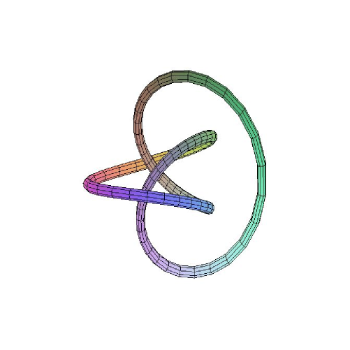
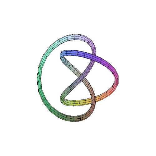
Figure 3. Morton’s trigonometric curve without tritangent planes (Example 4.4).

Figure 1 shows a picture (due to Frank Sottile [17, Fig. 3]) of the convex hull of the curve.

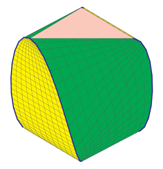
Figure 1. The convex hull of the curve $({\rm cos}(\theta),{\rm sin}(2\theta),{\rm cos}(3\theta))$ has two triangles and two non-linear surfaces patches of degree $3$ and $16$ in its boundary.

This picture shows the facets (maximal faces) of this convex body. There are two $2$-dimensional facets, namely the triangles whose vertices have parameters $\theta=0,\frac{2\pi}{3},\frac{4\pi}{3}$ and $\theta=\frac{\pi}{3},\pi,\frac{5\pi}{3}$. Further, we see two one-dimensional families of $1$-dimensional facets. These sweep out the yellow surface and the green surface in Figure 1. The boundary is the union of the two triangles and the two surfaces. Each triangle lies in a tritangent plane to the curve, while the $1$-dimensional facets are segments in stationary bisecant lines. The union of all stationary bisecant lines is the edge surface of the curve, as defined in Section 2. The lines in the quadratic cone $\{x^{2}-y^{2}-xz=0\}$ are also stationary bisecants to $C$, so this cone is a third component of the edge surface of $C$, but it does not contribute to the boundary of its convex hull. The tritangent planes and the edge surface are our primary objects of study.

The problem of computing the convex hull of a space curve is fundamental for non-linear computational geometry, but the literature on algorithms is surprisingly sparse. One exception is an article on geometric modeling by Seong et al. [19, §3] which describes the boundary in terms of stationary bisecants and tritangents, corresponding to our surfaces and triangles. This description of the boundary surface was also known to Sedykh [18] who undertook a detailed study of the singularities arising in the boundary of such a $3$-dimensional convex body.

Recent interest in computing convex hulls of algebraic varieties arose in the theory of semidefinite programming. We refer to the articles of Gouveia et al. [9], Henrion [12] and Netzer et al. [15] for details and references. Their aim is to represent the convex hull as the projection of a spectrahedron, or, algebraically, one seeks to find a lifted LMI representation for the convex hull. Such a representation always exists when the variety is a rational curve. This follows from the fact that every non-negative polynomial in one variable is a sum of squares. Its construction was explained in [12, §4-5] and in [17, §5].

Since trigonometric curves are rational, their convex hull has a lifted LMI representation. The convex hull of our curve is the following projection of a $6$-dimensional spectrahedron:

$$\hbox{{\rm Figure} \ref{fig:frank}}\,\,\,=\,\,\,\biggl{\{}(x,y,z)\in\mathbb{R}^{3}\,\,|\,\,\exists\,u,v,w\in\mathbb{R}\,:\,\begin{pmatrix}1&x+ui&v+yi&z+wi\\ x-ui&1&x+ui&v+yi\\ v-yi&x-vi&1&x+ui\\ z-wi&v-yi&x-ui&1\end{pmatrix}\,\succeq\,0\,\biggr{\}}.$$

Here $i=\sqrt{-1}$ and “$\succeq 0$” means that this Hermitian $4{\times}4$-matrix is positive semidefinite. A lifted LMI representation solves our problem from the point of view of convex optimization because it allows us to rapidly maximize any linear function over the curve. However, that formula is unsatisfactory from an algebro-geometric perspective because it reveals little information about boundary surfaces visible in Figure 1. Our goal is to present practical tools for computing the irreducible polynomials defining these surfaces, or at least their degrees.

It is quite easy to see that the yellow surface in Figure 1 has degree $3$ and is defined by

(1.3) $$z-4x^{3}+3x\,\,=\,\,0.$$

However, it is not obvious that the green surface has degree $16$ and its defining polynomial is

$$\tiny\begin{matrix}1024x^{16}-12032x^{14}y^{2}+52240x^{12}y^{4}-96960x^{10}y^{6}+56160x^{8}y^{8}+19008x^{6}y^{10}+1296x^{4}y^{12}+6144x^{15}z-14080x^{13}y^{2}z\\ -72000x^{11}y^{4}z+149440x^{9}y^{6}z+79680x^{7}y^{8}z+7488x^{5}y^{10}z+15360x^{14}z^{2}+36352x^{12}y^{2}z^{2}+151392x^{10}y^{4}z^{2}+131264x^{8}y^{6}z^{2}\\ +18016x^{6}y^{8}z^{2}+20480x^{13}z^{3}+73216x^{11}y^{2}z^{3}+105664x^{9}y^{4}z^{3}+23104x^{7}y^{6}z^{3}+15360x^{12}z^{4}+41216x^{10}y^{2}z^{4}+16656x^{8}y^{4}z^{4}\\ +6144x^{11}z^{5}+6400x^{9}y^{2}z^{5}+1024x^{10}z^{6}-26048x^{14}-135688x^{12}y^{2}+178752x^{10}y^{4}+124736x^{8}y^{6}-210368x^{6}y^{8}+792x^{4}y^{10}\\ +5184x^{2}y^{12}+432y^{14}-77888x^{13}z+292400x^{11}y^{2}z+10688x^{9}y^{4}z-492608x^{7}y^{6}z-67680x^{5}y^{8}z+21456x^{3}y^{10}z+2592xy^{12}z\\ -81600x^{12}z^{2}-65912x^{10}y^{2}z^{2}-464256x^{8}y^{4}z^{2}-192832x^{6}y^{6}z^{2}+31488x^{4}y^{8}z^{2}+6552x^{2}y^{10}z^{2}-40768x^{11}z^{3}-194400x^{9}y^{2}z^{3}\\ -196224x^{7}y^{4}z^{3}+14912x^{5}y^{6}z^{3}+8992x^{3}y^{8}z^{3}-20800x^{10}z^{4}-84088x^{8}y^{2}z^{4}-7360x^{6}y^{4}z^{4}+7168x^{4}y^{6}z^{4}-12480x^{9}z^{5}\\ -9680x^{7}y^{2}z^{5}+3264x^{5}y^{4}z^{5}-2624x^{8}z^{6}+760x^{6}y^{2}z^{6}+64x^{7}z^{7}+189649x^{12}+104700x^{10}y^{2}-568266x^{8}y^{4}+268820x^{6}y^{6}\\ +118497x^{4}y^{8}-42984x^{2}y^{10}-432y^{12}+62344x^{11}z-592996x^{9}y^{2}z+421980x^{7}y^{4}z+377780x^{5}y^{6}z-79748x^{3}y^{8}z-18288xy^{10}z\\ +104620x^{10}z^{2}+56876x^{8}y^{2}z^{2}+480890x^{6}y^{4}z^{2}-12440x^{4}y^{6}z^{2}-51354x^{2}y^{8}z^{2}-936y^{10}z^{2}+35096x^{9}z^{3}+181132x^{7}y^{2}z^{3}\\ +73800x^{5}y^{4}z^{3}-52792x^{3}y^{6}z^{3}-3780xy^{8}z^{3}-6730x^{8}z^{4}+52596x^{6}y^{2}z^{4}-19062x^{4}y^{4}z^{4}-5884x^{2}y^{6}z^{4}+y^{8}z^{4}+6008x^{7}z^{5}\\ +2516x^{5}y^{2}z^{5}-4324x^{3}y^{4}z^{5}+4xy^{6}z^{5}+2380x^{6}z^{6}-1436x^{4}y^{2}z^{6}+6x^{2}y^{4}z^{6}-152x^{5}z^{7}+4x^{3}y^{2}z^{7}+x^{4}z^{8}-305250x^{10}\\ +313020x^{8}y^{2}+174078x^{6}y^{4}-291720x^{4}y^{6}+74880x^{2}y^{8}+84400x^{9}z+278676x^{7}y^{2}z-420468x^{5}y^{4}z+20576x^{3}y^{6}z+40704xy^{8}z\\ -25880x^{8}z^{2}-76516x^{6}y^{2}z^{2}-148254x^{4}y^{4}z^{2}+77840x^{2}y^{6}z^{2}+5248y^{8}z^{2}-29808x^{7}z^{3}-49388x^{5}y^{2}z^{3}+23080x^{3}y^{4}z^{3}\\ +14560xy^{6}z^{3}+14420x^{6}z^{4}-7852x^{4}y^{2}z^{4}+9954x^{2}y^{4}z^{4}+568y^{6}z^{4}+848x^{5}z^{5}+92x^{3}y^{2}z^{5}+1164xy^{4}z^{5}-984x^{4}z^{6}+724x^{2}y^{2}z^{6}\\ -2y^{4}z^{6}+112x^{3}z^{7}-4xy^{2}z^{7}-2x^{2}z^{8}+140625x^{8}-270000x^{6}y^{2}+172800x^{4}y^{4}-36864x^{2}y^{6}-75000x^{7}z+36000x^{5}y^{2}z\\ +46080x^{3}y^{4}z-24576xy^{6}z-12500x^{6}z^{2}+49200x^{4}y^{2}z^{2}-19968x^{2}y^{4}z^{2}-4096y^{6}z^{2}+15000x^{5}z^{3}-10560x^{3}y^{2}z^{3}\\ -3072xy^{4}z^{3}-2250x^{4}z^{4}-1872x^{2}y^{2}z^{4}+768y^{4}z^{4}-520x^{3}z^{5}+672xy^{2}z^{5}+204x^{2}z^{6}-48y^{2}z^{6}-24xz^{7}+z^{8}.\end{matrix}$$

This paper is organized as follows. In Section 2 we apply known results from algebraic geometry to derive formulas for the number of tritangents and the degree of the edge surface of a smooth curve $C$ of degree $d$ and genus $g$ in $\mathbb{R}^{3}$. This characterizes the intrinsic algebraic complexity of computing the convex hull of $C$. In Section 3 we focus on trigonometric curves, which are compact of even degree $d$ and genus $g=0$. We describe an algebraic elimination method for computing their tritangents and edge surfaces. The method will be demonstrated for curves of degree $d=6$, which have $8$ tritangents and whose edge surface has degree $30$. If the curve is singular then that number drops, for instance to $16{+}3{+}2$ in the example above.

Freedman [8] asked in 1980 whether every generic smooth knotted curve $C$ in $\mathbb{R}^{3}$ must have a tritangent plane. Ballesteros-Fuster [3] and Morton [14] answered this to the negative by constructing trigonometric curves without tritangents. We reexamine the Morton curve in Section 4. Section 5 offers an in-depth study of the edge surface from the algebraic geometry perspective. We establish a refined degree formula that also works for curves with singularities, and we derive both old and new results on edge surfaces and their dual varieties.

The second hull of a knotted space curve, studied in [6], is strictly contained in the convex hull, but the algebraic surface defining their boundaries coincide. Thus, our algebraic recipes not only compute and represent the ordinary convex hull but they also yield the second hull.

Our study of the convex hull has been extended to higher-dimensional varieties in [16], which is a sequel to the present article. The paper [16] contains a characterization of the boundary of the convex hull of a compact real variety in affine space in terms of certain multiple strata in the dual variety. When the variety is a space curve, the important special case studied here, the dual variety of the edge surface is a double curve on the dual surface of the space curve, while the tritangent planes correspond to triple points on the dual surface.

2. Degree Formula for Smooth Curves

Let $C$ be a compact smooth real algebraic curve in $\mathbb{R}^{3}$. This means that the Zariski closure of $C$ in complex projective space $\mathbb{C}\mathbb{P}^{3}$ is a smooth projective curve, denoted $\bar{C}$. We define the degree and genus of $C$ to be the corresponding quantities for the complex curve $\bar{C}\subset\mathbb{C}\mathbb{P}^{3}$:

$$d={\rm degree}(C):={\rm degree}(\bar{C})\quad\hbox{and}\quad g={\rm genus}(C):={\rm genus}(\bar{C}).$$

Our object of study is the convex hull ${\rm conv}(C)$ of the real algebraic curve $C$. This is a compact, convex, semi-algebraic subset of $\mathbb{R}^{3}$, and its boundary $\partial{\rm conv}(C)$ is a semi-algebraic subset of pure dimension $2$ in $\mathbb{R}^{3}$. We wish to understand the structure of this boundary.

We define the algebraic boundary of the convex body ${\rm conv}(C)$ to be the $K$-Zariski closure of $\partial{\rm conv}(C)$ in complex affine space $\mathbb{C}^{3}$. Here $K$ is the subfield of $\mathbb{R}$ over which the curve $C$ is defined. The algebraic boundary is denoted $\partial_{a}{\rm conv}(C)$. This complex surface is usually reducible, and we identify it with its defining square-free polynomial in $K[x,y,z]$. Note that the algebraic boundary depends on the choice of the field $K$, and its degree is understood in the usual sense of algebraic geometry. All curves $C$ in our examples are defined over $K=\mathbb{Q}$.

Combining the description of the convex hull by Sedykh [18] and Seung et al. [19] with enumerative results of De Jonquières [1], Arrondo et al. [2] and Johnsen [13], we shall derive the following characterization of the expected factors of this polynomial and their degrees:

Theorem 2.1.

Let $C$ be a general smooth compact curve of degree $d$ and genus $g$ in $\mathbb{R}^{3}$. The algebraic boundary $\partial_{a}{\rm conv}(C)$ of its convex hull is the union of the edge surface and the tritangent planes. The edge surface is irreducible of degree $\,2(d-3)(d+g-1)$, and the number of complex tritangent planes equals $\,8\binom{d+g-1}{3}-8(d{+}g{-}4)(d{+}2g{-}2)+8g-8$.

We first explain some of the terms appearing in the statement, and then we embark on the proof. A plane $H$ in $\mathbb{C}\mathbb{P}^{3}$ is a tritangent plane of $\bar{C}$ if $H$ is tangent to $\bar{C}$ at three or more non-collinear points. For general curves, no plane $H$ can be tangent to four or more points on $\bar{C}$, so all tritangents touch the curve $\bar{C}$ in precisely three points. In the count above we assume that this is the case. In particular, the curve is not a plane curve. Among the tritangent planes are the affine spans of two-dimensional facets of ${\rm conv}(C)$, and generically such facets are triangles. Usually, not all tritangent planes will be defined over the real numbers, and only a subset of the real tritangent planes will correspond to triangle faces of $\partial{\rm conv}(C)$. Moreover, if $C$ is defined over $\mathbb{Q}$, we can use symbolic computation to compute the polynomial that defines the union of all tritangent planes. This is the Chow form in (4.2) below. The number of tritangent planes in Theorem 2.1 is the degree of that Chow form.

We define the edge surface of $C$ to be the union of all stationary bisecant lines in the sense of Arrondo et al. [2, §2]. To see what this means, let us consider any point $p$ in the boundary $\partial{\rm conv}(C)$ that does not lie in $C$ or in any $2$-dimensional face. Since every maximal face of a convex body is exposed, the boundary $\partial{\rm conv}(C)$ is the union of the exposed faces. We can thus choose a plane $H$ that exposes a face $F$ containing $p$. The face $F$ is not a polygon and it is not a vertex since $p\not\in C$. Therefore $F$ is one-dimensional, $H\cap C$ consists of two points $p_{1}$ and $p_{2}$, and $F$ is the edge between $p_{1}$ and $p_{2}$. The line $L$ spanned by $F$ is a stationary bisecant line. This means that $L$ is a bisecant line and that the tangent lines of $C$ at the intersection points $p_{1}$ and $p_{2}$ lie in a common plane, namely $H$. The edge surface may have several components, as we shall see in Example 2.3. As for tritangent planes, only a subset of the stationary bisecant lines correspond to $1$-dimensional facets of $\partial{\rm conv}(C)$, so the edge surface may have components that do not contribute to this boundary.

Figure 2 shows a smooth rational quartic curve $C$ and its edge surface. Here $d=4,g=0$, so Theorem 2.1 says that there are no tritangents and the edge surface has degree six. The surface is singular along the curve $C$, and ${\rm conv}(C)$ is visible in the center of the diagram.

Proof of Theorem 2.1.

The number of tritangent planes will be derived from De Jonquières’ formula [1, p. 359] for a smooth complex projective curve $\bar{C}$ of degree $d$ and genus $g$ in $\mathbb{C}\mathbb{P}^{r}$. Let $a=(a_{1},...,a_{k})$ and $n=(n_{1},...,n_{k})$ be vectors of positive integers with $\sum_{i=1}^{k}a_{i}n_{i}=d$. We assume that the $a_{i}$ are distinct and that $\,s:=d-\sum_{i=1}^{k}n_{i}\leq r$. The set of all hyperplanes that intersect $C$ in $d-s$ points, where $n_{i}$ are intersected with multiplicity $a_{i}$, is a variety $V_{a,n}$ in the dual space $(\mathbb{C}\mathbb{P}^{r})^{*}$. De Jonquières’ formula states the following: If the dimension of $V_{a,n}$ is $r-s$ then the degree of $V_{a,n}$ equals the coefficient of $t_{1}^{n_{1}}\cdots t_{k}^{n_{k}}$ in the polynomial

(2.1) $$(1+\sum_{i=1}^{k}a_{i}^{2}t_{i})^{g}\cdot(1+\sum_{i=1}^{k}a_{i}t_{i})^{d-s-g}.$$

This formula can be used to investigate the sets of planes that are tangent to a space curve $\bar{C}\subset\mathbb{C}\mathbb{P}^{3}$, so first we set $r=3$. The variety of planes tangent to $\bar{C}$ is the dual variety $\bar{C}^{*}$ of $C$ and is obtained by taking $a=(2,1),n=(1,d-2)$ and $s=1$. In this way we recover the result that the dual variety $\bar{C}^{*}$ is a surface of degree $2(d+g-1)$.

The variety of tritangent planes for a curve $\bar{C}\subset\mathbb{C}\mathbb{P}^{3}$ is obtained from (2.1) by setting $a=(2,1),n=(3,d-6)$ and $s=3$. The expected dimension of that variety is $r-s=0$. So, when the set of tritangent planes is finite then its cardinality is the coefficient of $t_{1}^{3}t_{2}^{d-6}$ in

$$(1+4t_{1}+t_{2})^{g}\cdot(1+2t_{1}+t_{2})^{d-3-g}.$$

That coefficient is found to be the desired quantity $\,8\binom{d+g-1}{3}-8(d{+}g{-}4)(d{+}2g{-}2)+8g-8$.

We argued above that the union of all $1$-dimensional facets of ${\rm conv}(C)$ is Zariski dense in a component of the surface of stationary bisecants. This surface is precisely the edge surface of $C$, as defined above. Arrondo et al. [2, §2] study the edge surface as the focal surface of the congruence of bisecant lines or secants to $C$. They derive the degree of this surface from [2, Propositions 1.7 and 2.1]. The desired formula $2(d-3)(d+g-1)$ is stated explicitly in the remark prior to Example 2.4 in [2, page 547]. See also [13, Remarks 5.1 and 5.2]. We also give a direct derivation in Proposition 5.1. This concludes the proof of Theorem 2.1. ∎

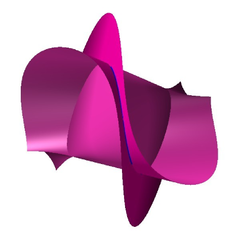
Figure 2. The edge surface of a rational quartic curve is irreducible of degree six.

Remark 2.2.

A general space curve $\bar{C}$ has a finite number of stalls. These are planes of third order contact at a point of the curve. They were studied by Banchoff, Gaffney and McCrory [4]. De Jonquières’ formula with $a=(4,1)$, $n=(1,d-4)$ and $s=3$ gives $4(d+3g-3)$ for the number of stalls. Related work is Sedykh’s classification [18] of six types of singularities. Each singularity type is exhibited by one of the two curves in Figures 1 and 3. ∎

As noted above, the formulas of Theorem 2.1 do not apply to plane curves. For space curves of degree $d\leq 5$, the formulas predict that the number of tritangent planes is zero.

Example 2.3 ($d=4,g=1$).

Consider a compact intersection $\,C=Q_{1}\cap Q_{2}\,$ of two general quadratic surfaces in $\mathbb{R}^{3}$. For instance, we could take $Q_{1}$ and $Q_{2}$ to be ellipsoids. The intersection curve $C$ is an elliptic space curve: it has genus $g=1$ and degree $d=4$. According to the formula in Theorem 2.1, the edge surface of $C$ has degree $8$. That surface is not irreducible but is the union of four quadratic cones. Indeed, the pencil of quadrics $\,Q_{1}+tQ_{2}\,$ contains precisely four singular quadrics, corresponding to the four real roots $t_{1},t_{2},t_{3},t_{4}$ of $f(t)={\rm det}(Q_{1}+tQ_{2})$. The rulings of these cones are all stationary bisecants to $C$. Their union is a surface of degree $8$, and this is the edge surface of our elliptic curve $C$.

In algebraic contexts, when $Q_{1}$ and $Q_{2}$ have coefficients in $\mathbb{Q}$, we use symbolic computation to determine the algebraic boundary $\,\partial_{a}{\rm conv}(C)$. Its defining polynomial is the resultant

$$\prod_{i=1}^{4}(Q_{1}+t_{i}Q_{2})(x,y,z)\,\,=\,\,{\rm resultant}_{t}\bigl{(}\,f(t),\,(Q_{1}+tQ_{2})(x,y,z)\,\bigr{)}.$$

We note that each of the four singular quadrics is the determinant of a linear symmetric $2{\times}2$-matrix polynomial $A_{i}x+B_{i}y+C_{i}z+D_{i}$. Placing these matrices along the diagonal in an $8{\times}8$ matrix of four $2{\times 2}$-blocks, we obtain a representation of ${\rm conv}(C)$ as spectrahedron. ∎

This example shows that the edge surface of a curve $C\subset\mathbb{R}^{3}$ can have multiple components even if its complexification $\bar{C}\subset\mathbb{C}\mathbb{P}^{3}$ is smooth and irreducible. We conjecture that at most one of these components is not a cone. For more information see Proposition 5.5 below.

3. Trigonometric Curves and their Edge Surfaces

By a trigonometric polynomial of degree $d$ we mean an expression of the form

(3.1) $$f(\theta)\,\,\,=\,\,\,\sum_{j=1}^{d/2}\alpha_{j}\,{\rm cos}(j\theta)\,\,+\,\,\sum_{j=1}^{d/2}\beta_{j}\,{\rm sin}(j\theta)\,\,+\,\,\gamma.$$

Here $d\in\mathbb{N}$ is tacitly assumed to be even and the coefficients $\,\alpha_{j},\beta_{j},\gamma\,$ can be arbitrary real numbers. We regard $f(\theta)$ as a real-valued function on the unit circle. A trigonometric space curve of degree $d$ is a curve parametrized by three trigonometric polynomials of degree $d$:

(3.2) $$C\,\,=\,\,\bigl{\{}\,\bigl{(}f_{1}(\theta),f_{2}(\theta),f_{3}(\theta)\bigr{)}\in\mathbb{R}^{3}\,:\,\theta\in[0,2\pi]\,\bigr{\}}.$$

The curve $C$ is the image of the circle under a polynomial map, so it is clearly compact.

For general coefficients $\alpha_{j},\beta_{j},\gamma$, the corresponding complex projective curve $\,\bar{C}\subset\mathbb{C}\mathbb{P}^{3}\,$ is smooth of degree $d$ and it has genus $g=0$. As in [12, §5], we can derive a polynomial parametrization of the algebraic curve $\bar{C}$ by means of the following change of coordinates:

(3.3) $$\cos(\theta)=\frac{x_{0}^{2}-x_{1}^{2}}{x_{0}^{2}+x_{1}^{2}}\quad\hbox{and}\quad\sin(\theta)=\frac{2x_{0}x_{1}}{x_{0}^{2}+x_{1}^{2}}.$$

Substituting into the right hand side of the equation

$$\begin{pmatrix}\phantom{-}{\rm cos}(j\theta)&{\rm sin}(j\theta)\,\\ -{\rm sin}(j\theta)&{\rm cos}(j\theta)\,\end{pmatrix}\,\,=\,\,\begin{pmatrix}\phantom{-}{\rm cos}(\theta)&{\rm sin}(\theta)\,\\ -{\rm sin}(\theta)&{\rm cos}(\theta)\,\end{pmatrix}^{j},$$

this change of variables expresses ${\rm cos}(j\theta)$ and ${\rm sin}(j\theta)$ as homogeneous rational functions of degree $0$ in $(x_{0}:x_{1})$. Their common denominator equals $\,g(x_{0},x_{1})=(x_{0}^{2}+x_{1}^{2})^{d}$. This gives

$$\bar{C}\,=\,\bigl{\{}(F_{0}(x):F_{1}(x):F_{2}(x):F_{3}(x))\,=\,(g:gf_{1}:gf_{2}:gf_{3})\in\mathbb{C}\mathbb{P}^{3}\,\,:\,\,(x_{0}:x_{1})\in\mathbb{C}\mathbb{P}^{1}\,\bigr{\}}.$$

In this section, we are interested in computing the compact convex body ${\rm conv}(C)$. The curve $\bar{C}$ is rational, and it is smooth for general choices of $\alpha_{j},\beta_{j},\gamma\in\mathbb{R}$. Theorem 2.1 implies:

Corollary 3.1.

The algebraic boundary of the convex hull of a general rational curve of degree $d$ consists of $8\binom{d-3}{3}$ tritangent planes and the edge surface of degree $2(d-3)(d-1)$.

In what follows we shall explain a symbolic elimination method for computing the defining polynomial of the edge surface of a rational curve $\bar{C}$. Our examples were computed with Macaulay2 [10]. The problem of finding the tritangent planes is addressed in the next section.

Our approach will involve the Grassmannian ${\rm Gr}(2,4)$, which parametrizes all lines in $\mathbb{C}\mathbb{P}^{3}$. We identify ${\rm Gr}(2,4)$ with the hypersurface in $\mathbb{C}\mathbb{P}^{5}$ that is cut out by the Plücker quadric

$$u_{01}u_{23}-u_{02}u_{13}+u_{03}u_{12}\,=\,0.$$

Consider any pair of points $p$ and $q$ on the curve $\bar{C}$. They are represented by points $x_{p}=(x_{p0}:x_{p1})$ and $x_{q}=(x_{q0}:x_{q1})$ in the parameter space $\mathbb{C}\mathbb{P}^{1}$. The secant line of $C$ through $p$ and $q$ is the line in $\mathbb{C}\mathbb{P}^{3}$ whose six Plücker coordinates $\,u_{ij}\,$ are the $2{\times}2$-minors of the matrix

$$\begin{pmatrix}\,F_{0}(x_{p})&F_{1}(x_{p})&F_{2}(x_{p})&F_{3}(x_{p})\,\\ \,F_{0}(x_{q})&F_{1}(x_{q})&F_{2}(x_{q})&F_{3}(x_{q})\,\\ \end{pmatrix}.$$

The six minors are polynomials of degree $2d$ in the coordinates $x_{pj}$ and $x_{qj}$, and they share the common factor $x_{p0}x_{q1}-x_{p1}x_{q0}$. Dividing each minor by this factor yields polynomials $u_{ij}$ of degree $2d-2$. They are bihomogeneous of degree $(d-1,d-1)$ in the $x_{pj}$ and $x_{qj}$, and they are invariant under permuting the points $p$ and $q$. We can write each polynomial $u_{ij}$ uniquely as a polynomial of degree $d-1$ in the three fundamental bihomogeneous invariants

(3.4) $$a\,=\,x_{p0}x_{q0}\,,\,\,b\,=\,x_{p1}x_{q1}\,,\,\,\,c\,=\,x_{p0}x_{q1}+x_{p1}x_{q0}.$$

This identifies the plane $\mathbb{C}\mathbb{P}^{2}$ with coordinates $(a:b:c)$ with the symmetric square of the parameter line $\mathbb{C}\mathbb{P}^{1}$ of our curve $\bar{C}$. We have constructed a polynomial map of degree $d-1$:

(3.5) $$\mathbb{C}\mathbb{P}^{2}\,\rightarrow\,{\rm Gr}(2,4)\subset\mathbb{C}\mathbb{P}^{5}\,\,,\,\,\,(a:b:c)\,\mapsto\,(u_{01}:u_{02}:u_{03}:u_{12}:u_{13}:u_{23}).$$

Geometrically, this represents the secant map from the symmetric square of the space curve $\bar{C}$ to the Grassmannian. The image of this map is a surface of degree $(d-1)^{2}$ in ${\rm Gr}(2,4)$.

The stationary bisecants to $\bar{C}$ are the secant lines between points $p,q$ such that the tangent lines to $\bar{C}$ at these points intersect. The tangent line at $p$ is defined by the partial derivatives

$$\begin{pmatrix}\frac{\partial}{\partial x_{p0}}F_{0}(x_{p})&\frac{\partial}{\partial x_{p0}}F_{1}(x_{p})&\frac{\partial}{\partial x_{p0}}F_{2}(x_{p})&\frac{\partial}{\partial x_{p0}}F_{3}(x_{p})\\ \rule{0.0pt}{15.0pt}\frac{\partial}{\partial x_{p1}}F_{0}(x_{p})&\frac{\partial}{\partial x_{p1}}F_{1}(x_{p})&\frac{\partial}{\partial x_{p1}}F_{2}(x_{p})&\frac{\partial}{\partial x_{p1}}F_{3}(x_{p})\\ \end{pmatrix}.$$

The secant line between the points $p$ and $q$ is stationary if the determinant of the matrix

(3.6) $$\begin{pmatrix}\frac{\partial}{\partial x_{p0}}F_{0}(x_{p})&\frac{\partial}{\partial x_{p0}}F_{1}(x_{p})&\frac{\partial}{\partial x_{p0}}F_{2}(x_{p})&\frac{\partial}{\partial x_{p0}}F_{3}(x_{p})\\ \rule{0.0pt}{15.0pt}\frac{\partial}{\partial x_{p1}}F_{0}(x_{p})&\frac{\partial}{\partial x_{p1}}F_{1}(x_{p})&\frac{\partial}{\partial x_{p1}}F_{2}(x_{p})&\frac{\partial}{\partial x_{p1}}F_{3}(x_{p})\\ \rule{0.0pt}{15.0pt}\frac{\partial}{\partial x_{q0}}F_{0}(x_{q})&\frac{\partial}{\partial x_{q0}}F_{1}(x_{q})&\frac{\partial}{\partial x_{q0}}F_{2}(x_{q})&\frac{\partial}{\partial x_{q0}}F_{3}(x_{q})\\ \rule{0.0pt}{15.0pt}\frac{\partial}{\partial x_{q1}}F_{0}(x_{q})&\frac{\partial}{\partial x_{q1}}F_{1}(x_{q})&\frac{\partial}{\partial x_{q1}}F_{2}(x_{q})&\frac{\partial}{\partial x_{q1}}F_{3}(x_{q})\\ \end{pmatrix}$$

vanishes. The extraneous factor $x_{p0}x_{q1}-x_{p1}x_{q0}$ appears with multiplicity $4$ in the determinant. Removing this factor of degree $8$ from the determinant, we obtain a symmetric polynomial of degree $4(d-3)$ in $x_{p}$ and $x_{q}$. As before, we now write the resulting expression as a polynomial $\Phi(a,b,c)$ of degree $2(d-3)$ in the three fundamental invariants (3.4).

The equation $\Phi(a,b,c)=0$ defines a curve of degree $2(d-3)$ in the plane $\mathbb{C}\mathbb{P}^{2}$ that parametrizes the symmetric square of $\bar{C}$. This is the curve of all stationary bisecant lines to $\bar{C}$. The image of this plane curve under the degree $d-1$ map (3.5) is a curve of degree $2(d-3)(d-1)$ in the Grassmannian ${\rm Gr}(2,4)$.

We can compute the ideal $I_{\Phi}\subset\mathbb{R}[u_{01},u_{02},u_{03},u_{12},u_{13},u_{23}]$ of this image curve using Gröbner-based elimination. Finally, the last step is to pass from the curve in ${\rm Gr}(2,4)$ to the corresponding ruled surface of the same degree in $\mathbb{C}\mathbb{P}^{3}$. We can do this by adding three more unknowns $x,y,z$ and by augmenting the ideal $I_{\Phi}$ with the four equations

(3.7) $$\begin{pmatrix}\phantom{-}0&\phantom{-}u_{23}&-u_{13}&\phantom{-}u_{12}\,\\ -u_{23}&\phantom{-}0&\phantom{-}u_{03}&-u_{02}\,\\ \phantom{-}u_{13}&-u_{03}&\phantom{-}0&\phantom{-}u_{01}\,\\ -u_{12}&\phantom{-}u_{02}&-u_{01}&\phantom{-}0\,\end{pmatrix}\cdot\begin{pmatrix}1\\ x\\ y\\ z\end{pmatrix}\,\,=\,\,\begin{pmatrix}0\\ 0\\ 0\\ 0\end{pmatrix}.$$

The resulting ideal lives in $\mathbb{R}[u_{01},u_{02},u_{03},u_{12},u_{13},u_{23},x,y,z]$. From that ideal, we eliminate the first six unknowns to arrive at a principal ideal in $\mathbb{R}[x,y,z]$. The polynomial which generates the principal elimination ideal is the defining equation of the edge surface of $C$.

Example 3.2 ($d=4,g=0$).

We consider the convex hull of a general trigonometric curve $C$ of degree four. There are no tritangents, so its algebraic boundary is just the edge surface. In contrast to the elliptic curves of Example 2.3, where the edge surface had four components, the edge surface of the rational quartic curve $C$ is irreducible of degree six. For example, let

(3.8) $$C\,:\,\theta\,\mapsto\,\bigl{(}{\rm cos}(\theta),{\rm sin}(\theta)+{\rm cos}(2\theta),{\rm sin}(2\theta)\bigr{)}.$$

This curve is smooth and it is cut out by one quadric and two cubics. Its prime ideal is

$$\bigl{\langle}3x^{2}-y^{2}+2xz-z^{2}-2y,\,2y^{3}-4xyz+2yz^{2}+2y^{2}+xz+z^{2}-4y,4xy^{2}+4xz^{2}-2xy-4yz-2x+z\bigr{\rangle}.$$

The degree $3$ map $\mathbb{C}\mathbb{P}^{2}\rightarrow{\rm Gr}(2,4)$ in (3.5) which parametrizes the secant lines is given by

$$\begin{matrix}u_{01}=-a^{2}c-c^{3}+2abc-b^{2}c,\qquad\qquad\,&u_{02}=a^{3}-4a^{2}c+ac^{2}-3a^{2}b+3ab^{2}-b^{3}+4b^{2}c-bc^{2},\\ u_{03}=2a^{3}{-}2ac^{2}{-}2a^{2}b{-}2ab^{2}{+}2b^{3}{-}2bc^{2},&u_{12}=a^{3}{-}3a^{2}c{+}c^{2}a{+}c^{3}{-}a^{2}b{-}ab^{2}{-}2cab{+}b^{3}{-}3b^{2}c{+}bc^{2},\\ u_{13}=2a^{3}{-}2ac^{2}{+}2a^{2}b{-}2ab^{2}{-}2b^{3}{+}2bc^{2},&\!u_{23}=2a^{3}-2ac^{2}+14a^{2}b+14ab^{2}-8abc+2b^{3}-2bc^{2}.\end{matrix}$$

The determinant (3.6) reveals that the curve of stationary bisecants in $\mathbb{C}\mathbb{P}^{2}$ is cut out by

$$\Phi(a,b,c)\quad=\quad a^{2}-2ab+4ac+b^{2}+4bc-c^{2}.$$

The image of this curve in $\,{\rm Gr}(2,4)\subset\mathbb{C}\mathbb{P}^{5}\,$ is a curve of degree six. Its homogeneous prime ideal is minimally generated by eight quadrics in $\mathbb{R}[u_{01},u_{02},u_{03},u_{12},u_{13},u_{23}]$. We next add the four equations in (3.7) to these eight quadrics, we saturate with respect to the irrelevant ideal $\langle u_{01},u_{02},u_{03},u_{12},u_{13},u_{23}\rangle$, and thereafter we eliminate the six $u_{ij}$’s. As result we find

$$16x^{6}-32x^{4}y^{2}+16x^{2}y^{4}-96x^{5}z-160x^{3}y^{2}z+192x^{4}z^{2}+16x^{2}y^{2}z^{2}-128x^{3}z^{3}+216x^{4}y+48x^{2}y^{3}$$

$$-8y^{5}+72x^{3}yz+88xy^{3}z-72x^{2}yz^{2}-8y^{3}z^{2}+72xyz^{3}-207x^{4}-138x^{2}y^{2}-23y^{4}{+}180x^{3}z{+}60xy^{2}z$$

$$-126x^{2}z^{2}-54y^{2}z^{2}+108xz^{3}-27z^{4}-36x^{2}y+4y^{3}-36xyz+108x^{2}+36y^{2}-108xz+27z^{2}.$$

This irreducible sextic, defining the edge surface of the curve (3.8), is shown in Figure 2. ∎

The next examples we shall examine are trigonometric curves $C$ of degree $d=6$. If a rational sextic curve $\bar{C}$ is smooth, then its edge surface is irreducible of degree $30$, and our algorithm above will generate the irreducible polynomial of degree $30$ in $\mathbb{R}[x,y,z]$. However, when the coefficients of $f_{1},f_{2},f_{3}$ in (3.2) are special, then the projective curve $\bar{C}$ may have singularities in $\mathbb{C}\mathbb{P}^{3}$, even if $C$ is smooth in $\mathbb{R}^{3}$. In those cases, the degree of the edge surface of $C$ drops below $30$, and the surface may even decompose into several components.

Example 3.3.

In the Introduction we discussed the special curve $\,\bigl{(}{\rm cos}(\theta),{\rm sin}(2\theta),{\rm cos}(3\theta)\bigr{)}$. The corresponding polynomial parametrization $\,\mathbb{C}\mathbb{P}^{1}\rightarrow\mathbb{C}\mathbb{P}^{3}\,$ of the projective curve $\bar{C}$ equals

$$\bigl{(}\,(x_{0}^{2}+x_{1}^{2})^{3}:(x_{0}^{2}-x_{1}^{2})(x_{0}^{2}+x_{1}^{2})^{2}:4(x_{0}^{2}-x_{1}^{2})(x_{0}^{2}+x_{1}^{2})x_{0}x_{1}:(x_{0}^{2}-x_{1}^{2})(x_{1}^{4}-14x_{1}^{2}x_{0}^{2}+x_{0}^{4})\,\bigr{)}.$$

This curve has two singular points. The double point $(1:0:0:0)$ lies hidden inside the convex hull in Figure 1, and the double point $(0:0:0:1)$ lies in the plane at infinity. Notice that the plane at infinity intersects the curve only in this singular point. Our algorithm finds six polynomials $u_{ij}(a,b,c)$ of degree five that define the secant map $\mathbb{C}\mathbb{P}^{2}\rightarrow{\rm Gr}(2,4)$, but now the curve of stationary bisecants turns out to be reducible:

$$\Phi\,\,\,=\,\,\,(a-b)\,c\,(3a^{4}-6a^{2}b^{2}+2a^{2}c^{2}+3b^{4}+2b^{2}c^{2}-c^{4}).$$

Its image in ${\rm Gr}(2,4)$ is a reducible curve whose three components have degrees $2$, $3$ and $16$. These translate into three irreducible components of the edge surface of $\bar{C}$. From the factor $c$ we obtain the cubic surface (1.3) which is yellow in Figure 1, and from the quartic factor of $\Phi$ we obtain the surface of degree $16$ which is green in Figure 1. Finally, the factor $a-b$ contributes the quadratic surface $\{x^{2}-y^{2}-xz=0\}$, which is not needed for $\partial{\rm conv}(C)$. ∎

Example 3.4.

Henrion [12, §5] discusses the trefoil knot with parametric representation

$$C\,:\,\theta\,\mapsto\,\bigl{(}\,{\rm cos}(\theta)+2\,{\rm cos}(2\theta),\,{\rm sin}(\theta)+2\,{\rm sin}(2\theta),\,2\,{\rm sin}(3\theta)\,\bigr{)}.$$

This rational sextic $\,\bar{C}\subset\mathbb{C}\mathbb{P}^{3}\,$ has one singular point at $(0:0:0:1)$. By running our algorithm, we find that the edge surface of the curve $C$ is irreducible of degree $27$. ∎

Example 3.5.

The following remarkable sextic curve $\bar{C}$ is due to Barth and Moore [5]:

$$\mathbb{C}\mathbb{P}^{1}\rightarrow\mathbb{C}\mathbb{P}^{3}\,,\,\,\,(x_{0}:x_{1})\mapsto\bigl{(}\,x_{0}^{6}-2x_{0}x_{1}^{5}\,:\,2x_{0}^{5}x_{1}+x_{1}^{6}\,:\,x_{0}^{4}x_{1}^{2}\,:\,x_{0}^{2}x_{1}^{4}\,\bigr{)}.$$

This curve is smooth in $\mathbb{C}\mathbb{P}^{3}$, so its edge surface should have the expected degree $30$. However, when we run our algorithm, its output is only one irreducible polynomial of degree $10$:

$$27x^{5}y^{5}+3125y^{10}-1875x^{2}y^{7}z+\cdots+27z^{5}-16y^{3}z.$$

This surprising output is not a contradiction. The edge surface of the curve $\bar{C}$ naturally carries a non-reduced structure of multiplicity three. The geometry of $\bar{C}$ is such that every stationary bisecant line is a trisecant line with all three tangents lying in the same plane. The curve $\bar{C}$ therefore has a one-dimensional family of planes that are tangent at three points. This family defines an irreducible curve $\Gamma$ of degree $6$ in the dual projective space $(\mathbb{C}\mathbb{P}^{3})^{*}$.

The curve $\bar{C}$ has no tritangent planes at all. Indeed, our definition of tritangent planes required the presence of non-collinear points of tangency. De Jonquières formula, which predicts $8$ tritangents, does not apply here. If we run the algorithm of Section 4 for computing all points $(\alpha:\beta:\gamma:\delta)\in(\mathbb{C}\mathbb{P}^{3})^{*}$ dual to tritangent planes then the output is the curve $\Gamma$.

We can construct a real compact model $C\subset\mathbb{R}^{3}$ of the Barth-Moore curve $\bar{C}$ by replacing the first coordinate in $\mathbb{C}\mathbb{P}^{3}$ with the sum of all four coordinates. That sum is a positive binary sextic, and the corresponding new hyperplane at infinity contains no real points. This curve is not trigonometric because $(x_{0}^{2}+x_{1}^{2})^{3}$ is not in the linear span of the four coordinates. ∎

4. Computing Tritangent Planes

According to Corollary 3.1, a general trigonometric curve $C$ of degree $d$ has $8\binom{d-3}{3}$ tritangent planes, and these account for the two-dimensional polygonal faces of ${\rm conv}(C)$. In this section, we explain how these planes can be computed symbolically. The focus of our exposition remains on sextic curves, where the expected number of tritangent planes is eight.

We work with the polynomial parameterization $(F_{0}(x):F_{1}(x):F_{2}(x):F_{3}(x))$ of the projective curve $\bar{C}$. Each $F_{i}(x)$ is a binary form of degree $d$ in $x=(x_{0},x_{1})$. We represent a plane in $\mathbb{C}\mathbb{P}^{3}$ by a linear equation $\,\alpha+\beta x+\gamma y+\delta z=0$. The corresponding point $(\alpha:\beta:\gamma:\delta)$ in the dual projective space $(\mathbb{C}\mathbb{P}^{3})^{*}$ represents the parameters of our problem. The plane is tangent to $\bar{C}$ at a point $p$ if the point $\,(x_{p0}:x_{p1})\in\mathbb{C}\mathbb{P}^{1}\,$ is a double root of the binary form

(4.1) $$\alpha F_{0}(x)\,+\,\beta F_{1}(x)\,+\,\gamma F_{2}(x)\,+\delta F_{3}(x).$$

We seek to compute the set $\mathcal{T}_{C}$ of all points $\,(\alpha:\beta:\gamma:\delta)\in(\mathbb{C}\mathbb{P}^{3})^{*}\,$ such that (4.1) has three double roots. The set $\mathcal{T}_{C}$ is finite, of cardinality $8\binom{d-3}{d}$, and we can compute its ideal using Gröbner-based elimination. An alternative representation of $\,\mathcal{T}_{C}\,$ is its Chow form

(4.2) $$\prod_{(\alpha:\beta:\gamma:\delta)\in\mathcal{T}_{C}}\!\!\!(\alpha+\beta x+\gamma y+\delta z).$$

If the $F_{i}(x)$ have coefficients in $\mathbb{Q}$ then so does the Chow form (4.2), which will typically be irreducible over $\mathbb{Q}$. The corresponding surface in $\mathbb{C}\mathbb{P}^{3}$ is the union of all tritangent planes, and these include the planes in $\mathbb{R}^{3}$ that are spanned by all $2$-dimensional facets of ${\rm conv}(C)$.

For small values of $d$, such as $d=6$, we use the following preprocessing step whose output facilitates computing $\mathcal{T}_{C}$ for all rational curves $C$ of degree $d$. Consider the binary form

$$G(x)\,\,\,=\,\,\,\sum_{i=0}^{d}\kappa_{i}\,x_{0}^{i}x_{1}^{d-i}$$

whose coefficients $\kappa_{i}$ are unknowns. We precompute the prime ideal $P_{d}$ of height $3$ in $\mathbb{Q}[\kappa_{0},\ldots,\kappa_{d}]$ whose variety consists of all binary forms $G(x)$ that have three double roots. Suppose we know a list of generators for $P_{d}$. For any particular curve $C$, we can then equate $G(x)$ with (4.1), and this gives an expression for $\kappa_{i}$ as a linear combination of $\alpha,\beta,\gamma$ and $\delta$. Substituting these expressions for each $\kappa_{i}$, $i=0,1,\ldots,d$, we obtain an ideal $P_{d,C}$ of height $3$ in $\mathbb{Q}[\alpha,\beta,\gamma,\delta]$. The complex projective variety of $P_{d,C}$ is the desired set $\mathcal{T}_{C}$, and we can compute the Chow form (4.2) from the generators of $P_{d,C}$ by a standard elimination process.

Remark 4.1 ($d=6$).

The prime ideal $P_{6}$ is minimally generated by $45$ quartics such as

$$16\kappa_{0}^{2}\kappa_{6}^{2}+8\kappa_{0}\kappa_{1}\kappa_{5}\kappa_{6}-4\kappa_{0}\kappa_{3}^{2}\kappa_{6}+\kappa_{1}^{2}\kappa_{5}^{2}\,,\,\,8\kappa_{0}^{2}\kappa_{5}\kappa_{6}+2\kappa_{0}\kappa_{1}\kappa_{5}^{2}-4\kappa_{0}\kappa_{2}\kappa_{3}\kappa_{6}+\kappa_{1}^{2}\kappa_{3}\kappa_{6}\,,\,\,\ldots$$

The variety of the ideal $P_{6}$ consists of all binary sextics that are squares of binary cubics,

$$\kappa_{0}x_{1}^{6}+\kappa_{1}x_{0}^{1}x_{1}^{5}+\kappa_{2}x_{0}^{2}x_{1}^{4}+\cdots+\kappa_{6}x_{0}^{6}\,\,=\,\,(\nu_{0}x_{1}^{3}+\nu_{1}x_{0}x_{1}^{2}+\nu_{2}x_{0}^{2}x_{1}+\nu_{3}x_{0}^{3})^{2},$$

and it is quick and easy to generate all $45$ generators of $P_{6}$ in a system like Macaulay2. ∎

We now discuss the ideal $P_{d,C}$ and the Chow form (4.2) for two examples from Section 3.

Example 4.2.

The systematic computation of the tritangent planes to the curve $C$ in Figure 1 is done as follows. First, the trigonometric parametrization $({\rm cos}(\theta),{\rm sin}(2\theta),{\rm cos}(3\theta))$ is made polynomial via (3.3), and the resulting binary form (4.1) is then found to be

$$(\alpha+\beta+\delta)x_{0}^{6}+4\gamma x_{0}^{5}x_{1}+(3\alpha+\beta-15\delta)x_{0}^{4}x_{1}^{2}+(3\alpha-\beta+15\delta)x_{0}^{2}x_{1}^{4}-4\gamma x_{0}x_{1}^{5}+(\alpha-\beta-\delta)x_{1}^{6}.$$

Substituting the coefficients for $\kappa_{0},\ldots,\kappa_{6}$ into the $45$ generators of $P_{6}$, we arrive at the ideal

$$P_{6,\gamma}\,\,= \langle\alpha-\delta,\beta,\gamma\rangle\,\cap\,\langle\alpha+\delta,\beta,\gamma\rangle\,\cap\,\ \langle\alpha+\beta-7\delta,\gamma^{2}+4\beta\delta,\gamma\delta,\delta^{2}\rangle$$

$$\,\cap\,\,\langle\alpha-\beta+7\delta,\gamma^{2}+4\beta\delta,\gamma\delta,\delta^{2}\rangle\,\,\cap\,\,\langle\alpha,\beta,\gamma,\delta\rangle^{4}.$$

The ideal $P_{6,\gamma}$ has two simple roots and two triple roots in $\mathbb{C}\mathbb{P}^{3}$, and its Chow form equals

$${\rm Chow}(\mathcal{T}_{C})\,\,=\,\,(z-1)(z+1)(x-1)^{3}(x+1)^{3}.$$

This is the degree eight equation which defines the tritangent planes to the curve $C$. ∎

Example 4.3.

Let $C$ be Henrion’s curve $\,({\rm cos}(\theta)+2\,{\rm cos}(2\theta),\,{\rm sin}(\theta)+2\,{\rm sin}(2\theta),\,2\,{\rm sin}(3\theta))\,$ in Example 3.4. Here the Chow form of tritangent planes to $C$ is found to factor as follows:

$$(z-2)(z+2)(12x^{3}-11x^{2}z-6x^{2}y+8xzy-36xy^{2}+z^{3}+4z^{2}y-7zy^{2}-6y^{3}-100x^{2}+16xz$$

$$-80xy+32z^{2}+36zy-92y^{2}-16x+292z-40y+752)(12x^{3}+11x^{2}z+6x^{2}y+8xzy-36xy^{2}-z^{3}$$

$$-4z^{2}y+7zy^{2}+6y^{3}-100x^{2}-16xz+80xy+32z^{2}+36zy-92y^{2}-16x-292z+40y+752).\qed$$

We end with a prominent example of a sextic trigonometric curve. Freedman asked in [8] whether every generic smooth knotted curve $C$ in $\mathbb{R}^{3}$ must have a tritangent plane. This question was answered negatively by Ballesteros and Fuster [3] and Morton [14]. Their counterexamples are trigonometric curves. What follows is Morton’s trefoil example.

Example 4.4.

Morton [14] constructed the following rational trigonometric curve:

$$C\,\,:\,\,\theta\,\,\mapsto\,\,\frac{1}{2-{\rm sin}(2\theta)}\bigl{(}{\rm cos}(3\theta),{\rm sin}(3\theta),{\rm cos}(2\theta)\,\bigr{)}$$

This is a trefoil knot in $\mathbb{R}^{3}$. The corresponding polynomial parametrization $\mathbb{C}\mathbb{P}^{1}\rightarrow\mathbb{C}\mathbb{P}^{3}$ is

$$(x_{0}:x_{1})\,\,\mapsto\,\,\begin{pmatrix}2(x_{0}^{4}+2x_{0}^{2}x_{1}^{2}+x_{1}^{4}-2x_{0}^{3}x_{1}+2x_{0}x_{1}^{3})(x_{0}^{2}+x_{1}^{2})\\ (x_{0}-x_{1})(x_{0}+x_{1})(x_{1}^{2}+4x_{0}x_{1}+x_{0}^{2})(x_{1}^{2}-4x_{0}x_{1}+x_{0}^{2})\\ 2x_{0}x_{1}(x_{0}^{2}-3x_{1}^{2})(3x_{0}^{2}-x_{1}^{2})\\ (2x_{0}x_{1}+x_{0}^{2}-x_{1}^{2})(x_{0}^{2}-x_{1}^{2}-2x_{0}x_{1})(x_{0}^{2}+x_{1}^{2})\end{pmatrix}.$$

We compute the ideal $P_{6,C}$ and its Chow form as described above. The result is

$$\begin{matrix}{\rm Chow}(\mathcal{T}_{C})\,\,=&\!\!\!(x^{2}+y^{2})^{2}\cdot\bigl{(}13225x^{4}+58880x^{3}y+91986x^{2}y^{2}-638976x^{2}z^{2}+13225y^{4}\\ &+58880xy^{3}-1148160xyz^{2}-638976y^{2}z^{2}+6230016z^{4}+449280x^{2}z\\ &-449280y^{2}z-409600x^{2}-736000xy-409600y^{2}-7987200z^{2}+2560000\bigr{)}.\end{matrix}$$

The large quartic factor is irreducible over $\mathbb{Q}$ but it decomposes over $\mathbb{R}$ into linear factors:

$$\begin{matrix}(1+0.339305\,x+0.211829\,y+1.248999\,z)\cdot(1-0.339305\,x-0.211829\,y+1.248999\,z)\cdot\\ (1+0.211829\,x+0.339305\,y-1.248999\,z)\cdot(1-0.211829\,x-0.339305\,y-1.248999\,z).\end{matrix}$$

Each of these four tritangent planes touches the curve $\bar{C}$ in one real point and in two imaginary points. This answers Freedman’s question: the real curve $C\subset\mathbb{R}^{3}$ has no tritangent planes. Hence the algebraic boundary $\partial_{a}{\rm conv}(C)$ consists only of the edge surface of $C$. We find that this surface decomposes (over $\mathbb{Q}$) into two components of degrees $10$ and $20$. ∎

5. Degree formulas for Smooth and Singular Curves

This section concerns the algebraic geometry of the edge surface. We present a self-contained derivation of its degree and the degrees of its curves of singularities. Our approach to these calculations uses a method that goes back to Cayley and Plücker. In particular, Cayley computed in [7] the degree of the curve dual to the edge surface, i.e. the number of planes through a general point that are tangent to the curve at two points. Our approach is based on two classical formulas: De Jonquières’ formula (2.1) and Hurwitz’ formula $R=2\delta+2g-2$ for the degree $R$ of the ramification of a surjective map of degree $\delta$ from a smooth curve of genus $g$ onto $\mathbb{C}\mathbb{P}^{1}$ (see [11, IV.2.4]). The degree formulas we find for smooth curves are not new. In recent years they appeared in the study by von zur Gathen [20] of secant spaces to space curves, in the classification of projection centers of plane projections by T. Johnsen [13], and in the study of the focal surface of a congruence of lines by Arrondo et al. [2]. The correction term for singular curves in Theorem 5.2 appears to be new.

The computation interprets the edge surface as the scroll of stationary bisecants to the curve $\bar{C}$. This scroll is a curve of secants, while the variety of all secants to $\bar{C}$ form a surface in the Grassmannian ${\rm Gr}(2,4)$. Let $S_{2}=S_{2}\bar{C}$ be the symmetric square of the curve $\bar{C}$. If $\bar{C}$ is singular, we first normalize, and take the symmetric square of the normalized curve, thus $S_{2}$ is a smooth surface. As in Section 3, our key object is the secant map $S_{2}\to{\rm Gr}(2,4),$ which maps a pair of points on $\bar{C}$ to the secant spanned by them. The image of this map is the secant surface. We thus consider the edge surface as a curve of stationary bisecants on $S_{2}$ mapped by the secant map into the Grassmannian. We shall determine the class of this curve and of the hyperplane section of the secant surface in the Néron-Severi group of $S_{2}$.

For a generic smooth curve of genus $g>0$, the Néron-Severi group of divisors on $S_{2}$ has rank two. It is generated by the class of $C_{p}=\{(p,q)|q\in C\}\subset S_{2}$ and half the class of the diagonal, which we denote by $\Delta$. If $\bar{C}$ has geometric genus $g$, then $\Delta^{2}=1-g$, while $C_{p}^{2}=C_{p}\cdot\Delta=1$. For rational curves $(g=0)$, we have $S_{2}=\mathbb{C}\mathbb{P}^{2}$ and the Néron-Severi group has rank $1$, generated by the class of a line which coincides with $C_{p}$ and $\Delta$. The class $H$ on $S_{2}$ of a hyperplane section of the secant surface is computed using the fact that the lines meeting a fixed line in $\mathbb{C}\mathbb{P}^{3}$ form a hyperplane section of ${\rm Gr}(2,4)\subset\mathbb{C}\mathbb{P}^{5}$. The number of secants through a point on $\bar{C}$ that intersect a fixed line is $d-1$, so $H\cdot C_{p}=d-1$. The projection of $\bar{C}$ from a fixed line has ramification at the points where the tangent meets this line. By Hurwitz’ formula, we have $\,H\cdot 2\Delta=2d+2g-2$, and hence $\,H\equiv dC_{p}-\Delta$.

The class $B$ on $S_{2}$ of the curve of stationary bisecants to $\bar{C}$ is computed similarly: Set $B\equiv aC_{p}+b\Delta$. By Hurwitz’ formula, there are $2(d-2)+2g-2$ stationary bisecant lines through every point, so $B\cdot C_{p}=a+b=2(d+g-3)$. Next, a tangent line at a point $p$ is a stationary bisecant line only if $\bar{C}$ has a plane of third order contact at $p$, i.e. a stall. By Remark 2.2 their number is $4(d+3g-3)$, so the intersection number of $B$ with the diagonal is $B\cdot 2\Delta=2a+2b(1-g)=4(d+3g-3)$. Hence $B\equiv 2(d+g-1)C_{p}-4\Delta$ when $g>0$. When $g=0$, we have $C_{p}=\Delta$, and $B\equiv 2(d-3)C_{p}$.

Proposition 5.1.

The degree of the edge surface of a general smooth space curve of degree $d$ and genus $g$ is $2(d-3)(d+g-1)$.

Proof.

The degree of the edge surface is computed by the number of stationary bisecants that intersect a general line, so it is $H\cdot B=2(d-1)(d+g-1)-4d+4(1-g)=2(d-3)(d+g-1)$. ∎

If $\bar{C}$ has singularities, then the secant map is not defined at the singular points. More precisely, it is rational on the symmetric square $S_{2}$ of the normalization, but it is not defined on the pairs of points that lie over the singular points on $\bar{C}$. The secant map may, however, be extended by a blowup of $S_{2}$ in the points corresponding to the singularities. If the singularities are ordinary nodes or cusps, in the sense that no plane has local intersection multiplicity more than $4$, then the degree of the edge surface may be computed as above.

Theorem 5.2.

The edge surface of a general irreducible space curve of degree $d$, geometric genus $g$, with $n$ ordinary nodes and $k$ ordinary cusps, has degree $2(d{-}3)(d{+}g{-}1)-2n-2k$. The cone of bisecants through each cusp has degree $d{-}2$ and is a component of the surface.

Proof.

Consider an ordinary node or an ordinary cusp on $\bar{C}$, and let $(p,q)$ (resp. $(p,p)$) be the point on $S_{2}$ corresponding to the points on the normalization of $\bar{C}$ lying over the node (resp. cusp). Let $\tilde{S}_{2}$ be the blowup $S_{2}$ in $(p,q)$ (resp. $(p,p)$) with exceptional divisor $E$, and let $C_{p}$ and $\Delta$ be the pullback of the respective classes from $S_{2}$. Let $B$ denote the class on $\tilde{S}_{2}$ of the total transform of the curve of stationary bisecants on $S_{2}$, and let $H$ denote the class on $\tilde{S}_{2}$ of a hyperplane section. Now, the tangent cone at the node (resp. cusp) spans a plane, the unique plane with intersection multiplicity $4$ at the singularity. The pencil of lines in this plane through the singular point form the image of the exceptional divisor $E$ under the secant map. This pencil forms a line in ${\rm Gr}(2,4)$, so $H\cdot E=1$. On the other hand, $H\cdot C_{p}=d$ and $H\cdot 2\Delta=2d+2g-2$ as before, by Hurwitz’ formula for the normalized curve. Therefore $H\equiv dC_{p}-\Delta-E$. Next, the strict transform of the curve of stationary bisecants on the blowup of $S_{2}$ clearly lies in the class of $B-aE$ for some positive integer $a$. The computations of $(B-aE)\cdot C_{p}$ and $(B-aE)\cdot 2\Delta$ are not changed from the argument prior to Proposition 5.1 since we work on the normalization of $\bar{C}$: A secant through the point $p$ belongs to the curve of stationary bisecants on $S_{2}$ only if the tangent at $p$ and the tangent at some other point on the secant span a plane, while a tangent line at $p$ is a stationary bisecant only if there is third order contact with the branch of $\bar{C}$ at $p$ with a plane.

For either singularity, the cone that contains the curve and has its vertex at the singularity has degree $d-2$. The corresponding curve in the blowup of $S_{2}$ lies in the class of $C_{p}-E$. The projection from a nodal (resp. cuspidal) tangent has degree $d-3$ and ramification (by Hurwitz) of degree $2(d+g-4)$. This degree counts the number of tangent lines that meet the projection center. Since the singularities are ordinary, none of these lines are tangent at the singularity. The cone curve and the curve of stationary bisecants intersect only away from $E$, and with intersection number $(B-aE)\cdot(C_{p}-E)=2(d+g-3)-a=2(d+g-4)$. Therefore $a=2$, and the degree of the edge surface drops by $2$ compared to a smooth curve.

When the singularity is a cusp, the tangent to the normalization at the cusp is contracted on $\bar{C}$, so any secant through the vertex is necessarily a stationary bisecant. This curve of secants form a cone of degree $d-2$ that is a component of the edge surface.

The arguments used in this computation depend only on the local data of the singularities, so, as long as the curve $\bar{C}$ is irreducible, the arguments extend to several nodes and cusps. ∎

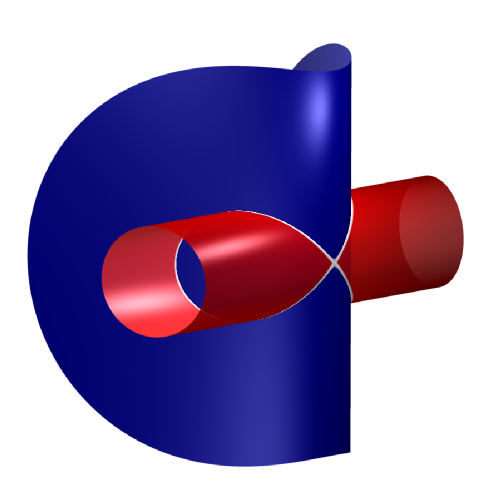
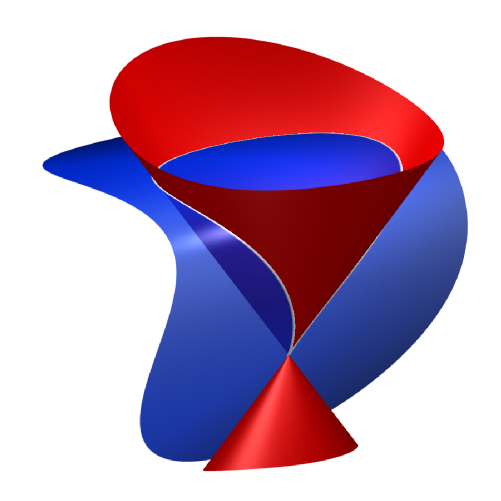
Figure 4. A nodal and a cuspidal rational quartic curve.

Example 5.3.

Figure 4 depicts the edge surface of a rational quartic curve with one ordinary singular point. The edge surface has degree $4$, the value obtained for $d=4,g=0,n+k=1$ in Theorem 5.2. It is the union of two quadric cones whose intersection equals the curve. If the singularity is an ordinary cusp, then one of the two quadrics has its vertex at the cusp. If the singularity is an ordinary node, then there are three quadric cones that contain the curve. One has its vertex in the node, but the edge surface is formed by the other two. ∎

Remark 5.4.

The singularities seen in some of our earlier examples are not ordinary, and Theorem 5.2 does not apply there. Henrion’s curve in Example 3.4 has a node in the plane at infinity. Both branches have intersection multiplicity three with the plane, so this node is not ordinary. The curve of stationary bisecants has a triple point at the corresponding point of $S_{2}=\mathbb{C}\mathbb{P}^{2}$. Thus the degree of the edge surface is reduced by three from the expected $30$.

The edge surface in Example 3.3 (shown in Figure 1) has three components, namely two cones of degree $2$ and $3$ respectively, and one component of degree $16$. The curve is the complete intersection of the two cones and has two double points. One double point is a node at the vertex of the quadric cone. The two branches at the point span a plane, but both branches have intersection multiplicity three with this plane so the node is not ordinary. The other double point lies in the plane at infinity and has two branches with a common tangent. The curve of stationary bisecants in $\mathbb{C}\mathbb{P}^{2}$ has three components, two lines corresponding to the two cones and one quartic curve. The secant map has two basepoints on $\mathbb{C}\mathbb{P}^{2}$, corresponding to the two singularities. The quartic curve has nodes at these basepoints. This explains the degree $16$ of the third component. ∎

These examples illustrate the general fact that the dual variety of the edge surface is a curve in the dual $\mathbb{C}\mathbb{P}^{3}$. This is well known, but for lack of reference we include a short proof. As above, cuspidal points on the curve $\bar{C}$ play a particular role. Here we take a cusp to mean any point $P\in\bar{C}$ such that the normalization $\tilde{C}\to\bar{C}$ is ramified over $P$, i.e. there is some point $Q\in\tilde{C}$ at which the normalization is not an immersion.

Proposition 5.5.

The variety dual to the edge surface of any space curve is a curve. In particular, each component of the edge surface is either a cone or the tangent developable of a curve. A cone is a component of the edge surface if and only if it is a cone of secants with vertex at a cusp, or the general ruling intersects the curve twice outside the vertex.

Proof.

Let $B_{0}$ be a component of the curve of stationary bisecants and let $\tilde{S}_{0}\to S_{0}$ be a minimal desingularization of the corresponding component $S_{0}$ of the edge surface. Then $\tilde{S}_{0}$ is a $\mathbb{C}\mathbb{P}^{1}$-bundle over the normalization $\tilde{B}_{0}$ of $B_{0}$ with a birational morphism onto the scroll $S_{0}$ that contains $\bar{C}$ in $\mathbb{C}\mathbb{P}^{3}$. Let $L$ be a general line in the ruling of this scroll, and assume first that $L$ does not pass through a cusp on $\bar{C}$. Then $L$ is a secant between distinct points on $\bar{C}$ whose tangents span a plane $P$. The pullback of this plane on $\tilde{S}_{0}$ is a curve $H$ that decomposes into $H=A+b\tilde{L}$ for some positive integer $b$ and is singular at the two points of tangency on the pullback $\tilde{L}$ of the line $L$.

Now, the curve $H$ is singular at a point of $\tilde{L}$ only if this is a point of intersection between the component $A$ and $\tilde{L}$ or $b>1$. But $H$ will intersect the general ruling in only one point, so $A$ cannot intersect $\tilde{L}$ in more than one point. Therefore $A+b\tilde{L}$ is singular along the whole ruling, i.e. $b>1$ and the plane $P$ is tangent to the scroll along $L$. If $L$ is a secant line through a cusp, the component of the edge surface is a cone of secants with vertex at a cusp, and the plane $P$ is tangent to the scroll along $L$. Thus the tangent plane is constant along each ruling, and the dual variety is a curve. To complete the proof, we consider biduality: Our scroll is the dual variety of a curve, so it is a cone if the curve is planar, and it is the tangent developable of the curve of osculating planes if the curve is not planar.

Since any cone has constant tangent planes along the rulings, a cone is a component of the edge surface for any curve that meet the general ruling in at least two distinct points outside the vertex. The only other way a cone could be a component of the edge surface is when the vertex is on the curve and the general ruling intersect the curve in one more point. To see this, we assume the vertex point is not a cusp on the curve. By assumption, each secant line from the vertex point is a stationary bisecant line, so there is a plane for each tangent to the curve that contains a tangent line at the vertex. Therefore the projection of the curve from a tangent line at the vertex is ramified everywhere on the curve. This is impossible over $\mathbb{C}$, and the proof is complete. ∎

Even when the curve $\bar{C}$ is generic and smooth, the edge surface is always highly singular [18]. First of all, the edge surface has multiplicity $2(d+g-3)$ along $\bar{C}$ itself. This number can be derived by applying Hurwitz’ formula to the projection from a tangent line. In addition, the singular locus of the edge surface has two further $1$-dimensional components. The edge surface is in general the tangent developable of a curve. A plane section of the edge surface have cusps at this curve, so the edge surface has a cuspidal edge along this curve. Finally the edge surface has in general an additional double curve, where two sheets of the surface intersect transversally. We compute the degrees of the cuspidal edge and of the double curve.

Proposition 5.6.

Let $\bar{C}$ be a general smooth curve of degree $d$ and genus $g$. The edge surface, which is reduced and irreducible, has multiplicity $2(d+g-3)$ along $\bar{C}$ and the 1-dimensional singular locus contains in addition a cuspidal edge of degree $6((d+g-3)^{2}-4g)$ and a double curve of degree $2d^{4}+4d^{3}g+2d^{2}g^{2}-18d^{3}-14dg^{2}-32d^{2}g+46d^{2}+52dg+8g^{2}-6d+64g-72$.

Proof.

The dual variety of the edge surface is a curve. The strict dual to this curve, the curve of osculating planes, is the cuspidal edge of the edge surface. Hence both the dual curve and the cuspidal edge are birational to the curve of stationary bisecants. Their common geometric genus is found to be $\gamma=2(d{+}g{-}2)(d{+}2g{-}4)+d-7g-4$ by adjunction on the symmetric square $S_{2}{\bar{C}}$. The degrees of these curves are computed by combining de Jonquières’ formula with a characterization of the cusps as in [13, Remarks 5.1 and 5.2]. The degree of the double curve is computed using the double point formula for a plane curve. The general plane section of the edge surface has geometric genus $\gamma$, it has $d$ points of multiplicity $2(d{+}g{-}3)$ and $6((d{+}g{-}3)^{2}-4g)$ cusps, so the formula for the number of double points follows. ∎

Acknowledgments. We are grateful to Oliver Labs and Philipp Rostalski for helping us with the diagrams. Figures 2 and 4 were drawn with Labs’ software Surfex, which is freely available at www.surfex.algebraicsurface.net. We thank Melody Chan, Joao Gouveia, Trygve Johnsen, Clint McCrory, Ragni Piene, Frank Sottile and Cynthia Vinzant for helpful discussions. Bernd Sturmfels was supported in part by NSF grant DMS-0757207.

References

• [1] E. Arbarello, M. Cornalba, P.A. Griffiths and J. Harris: Geometry of Algebraic Curves, Vol. I, Springer, New York, 1985.
• [2] E. Arrondo, M. Bertoloni and C. Turrini: A focus on focal surfaces, Asian J. Math. 5 (2001) 535–650.
• [3] J.J.N. Ballesteros and M.C.R. Fuster: Curves with no tritangent planes in space, Journal of Geometry 39 (1990) 120–129.
• [4] T. Banchoff, T. Gaffney and C. McCrory: Counting tritangent planes of space curves, Topology 24 (1985) 15–23.
• [5] W. Barth and R. Moore: On rational plane sextics with six tritangents. In Algebraic Geometry and Commutative Algebra, Vol. I, pages 45-58. Kinokuniya, Tokyo, 1988.
• [6] J. Cantarella, G. Kuperberg, R.B. Kusner and J.M. Sullivan: The second hull of a knotted curve, American Journal of Mathematics 125 (2003) 1335–1348.
• [7] A. Cayley: Mémoire sur le courbes à double courbure et les surfaces développables, J. de Math. Pures and Appl. 10 (1845) 245–250; also Math. Papers 1, 207-211.
• [8] M.H. Freedman: Planes triply tangent to curves with non-vanishing torsion, Topology 19 (1980) 1–8.
• [9] J. Gouveia, P. Parrilo and R. Thomas: Theta bodies of polynomial ideals, SIAM J. Optimization 20 (2010) 2097–2118.
• [10] D. Grayson and M.E. Stillman: Macaulay2, a software system for research in algebraic geometry, available at http://www.math.uiuc.edu/Macaulay2/.
• [11] R. Hartshorne: Algebraic Geometry, GTM 52, Springer, New York, 1977.
• [12] D. Henrion: Semidefinite representation of convex hulls of rational varieties, arXiv:0901.1821.
• [13] T. Johnsen: Plane projections of a smooth space curve, in Parameter Spaces, Banach Center Publications, Volume 36, (1996) 89-110.
• [14] H.R. Morton: Trefoil knots without tritangent planes, Bull. London Math. Soc. 23 (1991) 78–80.
• [15] T. Netzer, D. Plaumann and M. Schweighofer: Exposed faces of semidefinite representable sets, SIAM J.  Optimization 20 (2010) 1944–1955.
• [16] K. Ranestad and B. Sturmfels: The convex hull of a variety, to appear in the Julius Borcea Memorial Volume (eds. Petter Brändén, Mikael Passare, Mihal Putinar), Trends in Mathematics, Birkhäuser Verlag, arXiv:1004.3018.
• [17] R. Sanyal, F. Sottile and B. Sturmfels: Orbitopes, arXiv:0911.5436.
• [18] V.D. Sedykh: Singularities of the convex hull of a curve in $\mathbb{R}^{3}$, Functional Anal. Appl. 11 (1977) 72–73.
• [19] J.-K. Seong, G. Elber, J.K. Johnstone and M.-S. Kim: The convex hull of freeform surfaces, Computing 72 (2004) 171–183.
• [20] J. von zur Gathen: Secant spaces to curves, Canadian J. Math. 35 (1983) 589–612.